Three-cluster dynamics within the ab initio no-core shell model with continuum:
How many-body correlations and $\alpha$-clustering shape ⁶He

Abstract

We realize the treatment of bound and continuum nuclear systems in the proximity of a three-body breakup threshold within the ab initio framework of the no-core shell model with continuum. Many-body eigenstates obtained from the diagonalization of the Hamiltonian within the harmonic-oscillator expansion of the no-core shell model are coupled with continuous microscopic three-cluster states to correctly describe the nuclear wave function both in the interior and asymptotic regions. We discuss the formalism in detail and give algebraic expressions for the case of core+$n$+$n$ systems. Using similarity-renormalization-group evolved nucleon-nucleon interactions, we analyze the role of ⁴He+$n$+$n$ clustering and many-body correlations in the ground and low-lying continuum states of the Borromean ⁶He nucleus, and study the dependence of the energy spectrum on the resolution scale of the interaction. We show that ⁶He small binding energy and extended radii compatible with experiment can be obtained simultaneously, without recurring to extrapolations. We also find that a significant portion of the ground-state energy and the narrow width of the first $2^{+}$ resonance stem from many-body correlations that can be interpreted as core-excitation effects.

I Introduction

Since the first applications to the elastic scattering of nucleons on ⁴He and ¹⁰Be Nollett et al. (2007); Quaglioni and Navrátil (2008) roughly ten years ago, large-scale computations combined with new and sophisticated theoretical approaches Navrátil et al. (2016); Elhatisari et al. (2015); Hagen and Michel (2012) have enabled significant progress in the description of dynamical processes involving light and medium-mass nuclei within the framework of ab initio theory, i.e. by solving the many-body quantum-mechanical problem of protons and neutrons interacting through high-quality nuclear force models. This resulted in high-fidelity predictions for nucleon-nucleus Hagen and Michel (2012); Hupin et al. (2014); Langhammer et al. (2015); Lynn et al. (2016); Calci et al. (2016) and deuterium-nucleus Hupin et al. (2015) clustering phenomena and scattering properties, as well as predictive calculations of binary reactions, including the ³He$(\alpha,\gamma)^{7}$Be Neff (2011); Dohet-Eraly et al. (2016) and ⁷Be$(p,\gamma)^{8}$B Navrátil et al. (2011) radiative capture rates (important for solar astrophysics), and the ³H$(d,n)^{4}$He and ³He$(d,p)^{4}$He fusion processes Navrátil and Quaglioni (2012). A more recent breakthrough has enabled ab initio calculations of $\alpha$-$\alpha$ scattering Elhatisari et al. (2015), paving the way for the description of $\alpha$ scattering and capture reactions during the helium burning and later evolutionary phases of massive stars.

One of the main drivers of this progress has been the development of the no-core shell model with continuum, or NCSMC Baroni et al. (2013a, b). This is an ab initio framework for the description of the phenomena of clustering and low-energy nuclear reactions in light nuclei, which realizes an efficient description of both the interior and asymptotic configurations of many-body wave functions. The approach starts from the wave functions of each of the colliding nuclei and of the aggregate system, obtained within the ab initio no-core shell model (NCSM) Navrátil et al. (2000) by working in a many-body harmonic oscillator (HO) basis. It then uses the NCSM static solutions for the aggregate system and continuous ‘microscopic-cluster’ states, made of pairs of nuclei in relative motion with respect to each other, as an over-complete basis to describe the full dynamical solution of the system.

Recently, the NCSMC formalism was extended to the treatment of three-cluster dynamics, laying the groundwork for a comprehensive and unified description of systems characterized by ternary cluster structures, such as Borromean halo nuclei Jensen et al. (2004), as well as light-nuclei reactions with three nuclear fragments in either the entrance or exit channels. A few important examples of such reactions include the ⁴He$(2n,\gamma)^{6}$He radiative capture (one of the mechanism by which stars can overcome the instability of the five- and eight-nucleon systems and create heavier nuclei Käppeler et al. (1998)), and the ³H$(n,2n)^{2}$H and ³H$(t,2n)^{4}$He Casey et al. (2012); Sayre et al. (2013) fusion rates affecting the neutron spectrum generated in fusion experiments with deuterium-tritium fuel. Within the three-cluster extension of the NCSMC we studied how many-body correlations and $\alpha$+$n$+$n$ clustering shape the bound and continuum states of the Borromean ⁶He nucleus Romero-Redondo et al. (2016). More limited studies of this same system, based solely on the three-cluster portion of the NCSMC basis, were previously reported in Refs. Quaglioni et al. (2013) and Romero-Redondo et al. (2014). In this paper, we introduce in detail the general NCSMC formalism for the description of three-cluster dynamics, and present an extended discussion of the results published in Ref. Romero-Redondo et al. (2016) as well as additional results for the ⁶He nucleus.

The paper is organized as follows. In Sec. II, we introduce the NCSMC ansatz for systems characterized by a three-cluster asymptotic behavior, discuss the dynamical equations, and give the algebraic expressions of the overlap and Hamiltonian couplings between the discrete and continuous NCSMC basis states for the particular case of core+$n$+$n$ systems. We further discuss the procedure used for the solution of the three-cluster dynamical equations for bound and scattering states, and explain how we compute the probability density and matter and point-proton root-mean-square (rms) radii starting from the obtained NCSMC solutions for core+$n$+$n$ systems. The application of the approach to describe the ground and continuum states of the Borromean ⁶He nucleus is presented in Sec. III. Conclusions are drawn in Sec. IV, and detailed expressions for some of the most complex derivations are presented in Appendix.

II NCSMC with three-cluster channels

II.1 Ansatz

The intrinsic motion in a partial-wave of total angular momentum $J$, parity $\pi$ and isospin $T$ of a system of $A$ nucleons characterized by a three-cluster asymptotic behavior

$$|\Psi^{J^{\pi}T}\rangle =\sum_{\lambda}c^{J^{\pi}T}_{\lambda}|A\lambda J^{\pi}T\rangle$$ (1)

$$+\sum_{\nu}\iint dx\,dy\,x^{2}\,y^{2}\,G_{\nu}^{J^{\pi}T}(x,y)\,{\mathcal{A}}_{\nu}\,|\Phi^{J^{\pi}T}_{\nu xy}\rangle\,,$$

where $c^{J^{\pi}T}_{\lambda}$ and $G_{\nu}^{J^{\pi}T}(x,y)$ are discrete and continuous variational amplitudes, respectively, $|A\lambda J^{\pi}T\rangle$ is the $\lambda$-th (antisymmetric) $A$-nucleon eigenstate of the composite system in the $J^{\pi}T$ channel obtained working within the square-integrable many-body HO basis of the ab initio NCSM Navrátil et al. (2000), and

$$|\Phi^{J^{\pi}T}_{\nu xy}\rangle= \Big{[}\Big{(}|A-a_{23}~{}\alpha_{1}I_{1}^{\pi_{1}}T_{1}\rangle\left(|a_{2}\,\alpha_{2}I_{2}^{\pi_{2}}T_{2}\rangle|a_{3}\,\alpha_{3}I_{3}^{\pi_{3}}T_{3}\rangle\right)^{(s_{23}T_{23})}\Big{)}^{(ST)}\left(Y_{\ell_{x}}(\hat{\eta}_{23})Y_{\ell_{y}}(\hat{\eta}_{1,23})\right)^{(L)}\Big{]}^{(J^{\pi}T)}$$

$$\times\frac{\delta(x-\eta_{23})}{x\eta_{23}}\frac{\delta(y-\eta_{1,23})}{y\eta_{1,23}}$$ (2)

are continuous channel states (first introduced in Ref. Quaglioni et al. (2013)) describing the organization of the nucleons into three clusters of mass numbers $A-a_{23}$, $a_{2}$, and $a_{3}$ ($a_{23}=a_{2}+a_{3}<A$), respectively. Finally, the operator ${\mathcal{A}}_{\nu}$ is an appropriate intercluster antisymmetrizer introduced to guarantee the exact preservation of the Pauli exclusion principle.

In Eq. (2), $|A-a_{23}~{}\alpha_{1}I_{1}^{\pi_{1}}T_{1}\rangle$, $|a_{2}\,\alpha_{2}I_{2}^{\pi_{2}}T_{2}\rangle$ and $|a_{3}\,\alpha_{3}I_{3}^{\pi_{3}}T_{3}\rangle$ represent the microscopic (antisymmetric) wave functions of the three nuclear fragments, which are also obtained within the NCSM. They are labeled by the angular momentum, parity, isospin and energy quantum numbers $I_{i}^{\pi_{i}}$, $T_{i}$, and $\alpha_{i}$, respectively, with $i=1,2,3$. Additional quantum numbers characterizing the basis states (2) are the spins $\vec{s}_{23}=\vec{I}_{2}+\vec{I}_{3}$ and $\vec{S}=\vec{I}_{1}+\vec{s}_{23}$, the orbital angular momenta $\ell_{x}$, $\ell_{y}$ and $\vec{L}=\vec{\ell}_{x}+\vec{\ell}_{y}$, and the isospin $\vec{T}_{23}=\vec{T}_{2}+\vec{T}_{3}$. In our notation, all these quantum numbers are grouped under the cumulative index $\nu=\{A-a_{23}\,\alpha_{1}I_{1}^{\pi_{1}}T_{1};$ $a_{2}\,\alpha_{2}I_{2}^{\pi_{2}}T_{2};$ $a_{3}\,\alpha_{3}I_{3}^{\pi_{3}}T_{3};$ $s_{23}\,T_{23}\,S\,\ell_{x}\,\ell_{y}\,L\}$. Further, the inter-cluster relative motion is described with the help of the Jacobi coordinates $\vec{\eta}_{1,23}$ and $\vec{\eta}_{23}$ where

$$\vec{\eta}_{1,23} =\eta_{1,23}\hat{\eta}_{1,23}$$ (3)

$$=\sqrt{\tfrac{a_{23}}{A(A-a_{23})}}\sum_{i=1}^{A-a_{23}}\vec{r}_{i}-\sqrt{\tfrac{A-a_{23}}{A\,a_{23}}}\sum_{j=A-a_{23}+1}^{A}\vec{r}_{j}$$

is the relative vector proportional to the separation between the center of mass (c.m.) of the first cluster and that of the residual two fragments, and

$$\vec{\eta}_{23} =\eta_{23}\hat{\eta}_{23}$$ (4)

$$=\sqrt{\tfrac{a_{3}}{a_{23}\,a_{2}}}\sum_{i=A-a_{23}+1}^{A-a_{3}}\vec{r}_{i}-\sqrt{\tfrac{a_{2}}{a_{23}\,a_{3}}}\sum_{j=A-a_{3}+1}^{A}\vec{r}_{j}$$

is the relative coordinate proportional to the distance between the centers of mass of cluster 2 and 3 (see Fig. 1), where $\vec{r}_{i}$ denotes the position vector of the $i$-th nucleon.

The NCSM eigenstates appearing in Eqs. (1) and (2) are obtained by diagonalizing the $A$-, $(A-a_{23})$-, $a_{2}$-, and $a_{3}$-nucleon intrinsic Hamiltonians within complete sets of many-body HO basis states, the size of which is defined by the maximum number $N_{\rm max}$ of HO quanta above the lowest configuration shared by the nucleons. The same HO frequency $\hbar\Omega$ is used for the composite nucleus and all three clusters, and the model-space size $N_{\rm max}$ is identical (differs by one) for states of the same (opposite) parity.

Figure 1: (Color online) We show the Jacobi coordinates $\vec{\eta}_{1,23}$ (proportional to the vector between the c.m. of the first cluster and that of the residual two fragments) and $\vec{\eta}_{23}$ (proportional to the vector between the c.m. of clusters 2 and 3). In the figure, a case with three clusters of four, two and one nucleons are shown, however the formalism is completely general and can be used to describe any three cluster configuration.

The NCSMC ansatz of Eq. (1) can be seen as an example of generalized cluster expansion containing single and three-body cluster terms. In general such expansion could also contain binary-cluster and/or even higher-body cluster terms, chosen according to the particle-decay channels characterizing the system under consideration. It allows to capture, within a unified consistent framework, both the single-particle dynamics and microscopic-cluster picture of nuclei. For systems in the proximity of a three-body particle-decay channel, but away from two- or higher-body thresholds, Eq. (1) represents a good ansatz, which converges to the exact solution as $N_{\rm max}\to\infty$. In particular, the square-integrable NCSM eigenstates $|A\lambda J^{\pi}T\rangle$ of the composite nucleus provide an efficient description of the short- to medium-range $A$-body structure of the wave function, while the microscopic three-cluster channels $|\Phi^{J^{\pi}T}_{\nu xy}\rangle$ make the theory able to handle the long-range and scattering physics of the system.

II.2 Dynamical equations

Adopting the ansatz (1) for the many-body wave function and working in the model space spanned by the set of discrete $|A\,\lambda J^{\pi}T\rangle$ and continuous ${\mathcal{A}}_{\nu}|\Phi^{J^{\pi}T}_{\nu xy}\rangle$ basis states, the Schrödinger equation in each partial wave channel can be mapped onto a generalized eigenvalue problem, schematically given by

$$\left({\mathbb{H}}-E\,{\mathbb{N}}\right){\mathbb{C}}=0\,,$$ (5)

where $E$ is the total energy of the system in the c.m. reference frame. To simplify the formalism, the specification of the partial wave under consideration ($J^{\pi}T$ ) is now (and in the remainder of the paper) implied. In Eq. (5)

$${\mathbb{H}}^{\lambda\lambda^{\prime}}_{\nu xy,\nu^{\prime}x^{\prime}y^{\prime}}=\left(\begin{array}[]{lcl}E_{\lambda}\delta_{\lambda\lambda^{\prime}}&&\bar{h}_{\lambda\nu^{\prime}}(x^{\prime},y^{\prime})\\[5.69054pt] \bar{h}_{\lambda^{\prime}\nu}(x,y)&&\overline{\mathcal{H}}_{\nu\nu^{\prime}}(x,y,x^{\prime},y^{\prime})\end{array}\right)\,,$$ (8)

and

$${\mathbb{N}}^{\lambda\lambda^{\prime}}_{\nu xy,\nu^{\prime}x^{\prime}y^{\prime}}=\left(\begin{array}[]{lcl}\delta_{\lambda\lambda^{\prime}}&&\bar{g}_{\lambda\nu^{\prime}}(x^{\prime},y^{\prime})\\[5.69054pt] \bar{g}_{\lambda^{\prime}\nu}(x,y)&&\Delta_{\nu\nu^{\prime}}(x,y,x^{\prime},y^{\prime})\end{array}\right)\,,$$ (11)

are two-by-two block-matrices representing, respectively, the NCSMC Hamiltonian and norm (or overlap) kernels, i.e. the matrix elements of the Hamiltonian and identity operators over the set of discrete and continuous basis states spanning the model space. Specifically, the upper diagonal blocks are NCSM eigenstates of the $A$-nucleon Hamiltonian and are trivially given by the diagonal matrix of the corresponding eigenenergies $E_{\lambda}$ and the identity matrix, respectively. Analogously the lower diagonal blocks

$$\overline{\mathcal{H}}_{\nu\nu^{\prime}}(x,y,x^{\prime},y^{\prime}) =\left[{\mathcal{N}}^{-\frac{1}{2}}\mathcal{H}{\mathcal{N}}^{-\frac{1}{2}}\right]_{\nu\nu^{\prime}}(x,y,x^{\prime},y^{\prime})\,,$$ (12)

$${\Delta}_{\nu\nu^{\prime}}(x,y,x^{\prime},y^{\prime}) =\delta_{\nu\nu^{\prime}}\frac{\delta(x-x^{\prime})}{xx^{\prime}}\frac{\delta(y-y^{\prime})}{yy^{\prime}}\,,$$ (13)

are orthonormalized integration kernels obtained from the Hamiltonian and overlap matrix elements evaluated on the continuous basis states ${\mathcal{A}}_{\nu}|\Phi^{J^{\pi}T}_{\nu xy}\rangle$, i.e. $\mathcal{H}_{\nu\nu^{\prime}}(x,y,x^{\prime},y^{\prime})$ and $\mathcal{N}_{\nu\nu^{\prime}}(x,y,x^{\prime},y^{\prime})$. Detailed expressions for these kernels can be found in Ref. Quaglioni et al. (2013), where we introduced the formalism for the description of three-cluster dynamics based solely on expansions over three-cluster channels states of the type of Eq. (2).

The off-diagonal blocks of Eqs. (8) and (11) are given by the couplings between the discrete and continuous sectors of the basis, with the cluster form factor, $\bar{g}_{\lambda\nu}(x,y)=[g{\mathcal{N}}^{-\frac{1}{2}}]_{\lambda\nu}(x,y)$, and coupling form factor, $\bar{h}_{\lambda\nu}(x,y)=[h{\mathcal{N}}^{-\frac{1}{2}}]_{\lambda\nu}(x,y)$, defined in terms of the matrix elements

$$g_{\lambda\nu}(x,y) =\langle A\,\lambda J^{\pi}T|{\mathcal{A}}_{\nu}|\Phi^{J^{\pi}T}_{\nu xy}\rangle\,,$$ (14)

$$h_{\lambda\nu}(x,y) =\langle A\,\lambda J^{\pi}T|H{\mathcal{A}}_{\nu}|\Phi^{J^{\pi}T}_{\nu xy}\rangle\,,$$ (15)

where $H$ is the microscopic $A$-nucleon Hamiltonian. The general derivation of these three-cluster form factors is outlined in Sec. II.3, together with their algebraic expressions for the specialized case in which the two lighter fragments are single nucleons.

Finally,

$${\mathbb{C}}^{\lambda}_{\nu xy}=\left(\begin{array}[]{c}c_{\lambda}\\ \chi_{\nu}(x,y)\end{array}\right)$$ (18)

is the vector of the expansion ‘coefficients’, where the relative wave functions $\chi_{\nu}(x,y)$ are related to the initial unknown continuous amplitudes through

$$G_{\nu}(x,y)=[{\mathcal{N}}^{-\frac{1}{2}}\chi]_{\nu}(x,y).$$ (19)

These are obtained by solving the NCSMC dynamical equations as discussed in Sec. II.4.

II.3 Form factors

In this section we discuss in more detail the derivation of the form factors in configuration space introduced in Sec. II.2, starting with the coupling form factor $h_{\lambda\nu}(x,y)$ of Eq. (15). This can be expressed in terms of the cluster form factor $g_{\lambda\nu}(x,y)$ and three potential form factors

$$v^{Q}_{\lambda\nu}(x,y) =\langle A\,\lambda J^{\pi}T|{\mathcal{A}}_{\nu}{\mathcal{V}}^{Q}|\Phi^{J^{\pi}T}_{\nu xy}\rangle\,,$$ (20)

with $Q$ a generic notation for either $1,23$ or $23$ or $3N$, as

$$h_{\lambda\nu}(x,y) =\left(T_{\rm rel}+\bar{V}_{\rm C}+E_{\alpha_{1}}+E_{\alpha_{2}}+E_{\alpha_{3}}\right)g_{\lambda\nu}(x,y)$$

$$\phantom{=}+v^{1,23}_{\lambda\nu}(x,y)+v^{23}_{\lambda\nu}(x,y)+v^{3N}_{\lambda\nu}(x,y)\,.$$

The above expression was obtained by separating the microscopic $A$-nucleon Hamiltonian into its relative-motion, average Coulomb and clusters’ components according to

$$H=T_{\rm rel}+\bar{V}_{C}+{\mathcal{V}}_{\rm rel}+H_{(A-a_{23})}+H_{(a_{2})}+H_{(a_{3})}\,,$$ (22)

and taking advantage of the fact that the antisymmetrization operator commutes with $H$. $T_{\rm rel}$ is the relative kinetic energy operator for the three-body system, $\bar{V}_{\rm C}=\bar{V}^{12}_{\rm C}+\bar{V}^{13}_{\rm C}+\bar{V}^{23}_{\rm C}$ is the sum of the pairwise average Coulomb interactions among the three clusters, and $E_{\alpha_{i}}$ is the eigenenergy of the $i$-th cluster, obtained by diagonalizing their respective intrinsic Hamiltonians, $H_{(A-a_{23})}$, $H_{(a_{2})}$ and $H_{(a_{3})}$. Further, ${\mathcal{V}}_{\rm rel}={\mathcal{V}}^{1,23}+{\mathcal{V}}^{23}+{\mathcal{V}}^{3N}$ denotes the relative potential, with

$${\mathcal{V}}^{1,23} =\sum_{i=1}^{A-a_{23}}\sum_{j=A-a_{23}+1}^{A}\left(V^{NN}_{ij}-\frac{\bar{V}^{12}_{\rm C}+\bar{V}^{13}_{\rm C}}{(A-a_{23})a_{23}}\right)\,,$$ (23)

$${\mathcal{V}}^{23} =\sum_{k=A-a_{23}+1}^{A-a_{3}}\sum_{l=A-a_{3}+1}^{A}\left(V^{NN}_{kl}-\frac{\bar{V}^{23}_{\rm C}}{a_{2}a_{3}}\right)\,,$$ (24)

and ${\mathcal{V}}^{3N}$ the inter-cluster interaction due to the three-nucleon force, which in general is part of a realistic Hamiltonian. In Eqs. (23) and (24), the notation $V^{NN}$ stands for the nuclear plus point-Coulomb two-body potential. We note that ${\mathcal{V}}_{\rm rel}$ is a short-range operator. Indeed, because of the subtraction of $\bar{V}_{\rm C}$, the overall Coulomb contribution decreases as the inverse square of the distances between pairs of clusters.

In the present paper we will consider only the nucleon-nucleon ($NN$) component of the inter-cluster interaction and disregard, for the time being, the term ${\mathcal{V}}^{3N}$. The inclusion of the three-nucleon force into the formalism, although computationally much more involved, is straightforward and will be the matter of future investigations. In the remainder of the paper, we will also omit the average Coulomb potential $\bar{V}_{C}$, which is null for neutral systems such as the ⁴He+$n$+$n$ investigated here. The treatment of charged system is nevertheless possible (at least in an approximate way) and can be implemented along the same lines of Ref. Descouvemont et al. (2006).

The use of Jacobi coordinates and translational invariant NCSM eigenstates of the $A$-nucleon system and microscopic-cluster states represents the ‘natural’ choice for the computation of the configuration-space form factors of Eqs. (14) and (20). However, such a relative-coordinate formalism is only practical for few-nucleon systems. To access p-shell nuclei, it is more efficient to work with single-particle coordinates and Slater-determinant (SD) basis states. As we outline in the following, the unique properties of the HO basis allows us to work with SD functions and still preserve the translational invariance of the form factors.

In a first step, we compute matrix elements analogous to Eqs. (14) and (20) but evaluated in an HO SD basis, i.e.

$${\vphantom{\langle A\,\lambda J^{\pi}T|{\mathcal{O}}_{\rm t.i.}|\Phi^{J^{\pi}T}_{\gamma n_{x}n_{y}}\rangle}}_{\rm SD}{\langle A\,\lambda J^{\pi}T|{\mathcal{O}}_{\rm t.i.}|\Phi^{J^{\pi}T}_{\gamma n_{x}n_{y}}\rangle}_{\rm SD}\,,$$ (25)

where ${\mathcal{O}}_{\rm t.i.}={\mathcal{A}}_{\nu},\,{\mathcal{A}}_{\nu}{\mathcal{V}}^{1,23},\,{\mathcal{A}}_{\nu}{\mathcal{V}}^{23}$ is a translational invariant operator. The SD NCSM eigenstates of the $A$-nucleon system factorize into the product of their translational-invariant counterparts with the $0\hbar\Omega$ HO motion of their c.m.  coordinate $\vec{R}^{(A)}_{\rm c.m.}$,

$$|A\lambda J^{\pi}T\rangle_{\rm SD}=|A\lambda J^{\pi}T\rangle\,R_{00}({R}^{(A)}_{\rm c.m.})Y_{00}(\hat{R}^{(A)}_{\rm c.m.})\,.$$ (26)

At the same time, the kets in Eq. (25) are a set of HO three-cluster channel states, defined as

$$|\Phi_{\gamma n_{x}n_{y}}^{J^{\pi}T}\rangle_{\rm SD}= \left[\left(|A-a_{23}~{}\alpha_{1}I_{1}^{\pi_{1}}T_{1}\rangle_{\rm SD}\left(Y_{\ell_{x}}(\hat{\eta}_{23})\left(|a_{2}\alpha_{2}I_{2}^{\pi_{2}}T_{2}\rangle|a_{3}\alpha_{3}I_{3}^{\pi_{3}}T_{3}\rangle\right)^{(s_{23}T_{23})}\right)^{(J_{23}T_{23})}\right)^{(ZT)}Y_{\ell_{y}}(\hat{R}^{a_{23}}_{\rm c.m.})\right]^{(J^{\pi}T)}$$

$$\times R_{n_{x}\ell_{x}}(\eta_{23})R_{n_{y}\ell_{y}}({R}^{a_{23}}_{\rm c.m.})\,,$$ (27)

describing the motion of the heaviest of the two clusters and of the system formed by the second and third clusters in the ‘laboratory’ reference frame. Here

$$\vec{R}^{(A-a_{23})}_{\rm c.m.}=R^{(A-a_{23})}_{\rm c.m.}\hat{R}^{(A-a_{23})}_{\rm c.m.}=\frac{1}{\sqrt{A-a_{23}}}\sum_{i=1}^{A-a_{23}}\vec{r}_{i}\,,$$ (28)

$$\vec{R}^{(a_{23})}_{\rm c.m.}=R^{(a_{23})}_{\rm c.m.}\hat{R}^{(a_{23})}_{\rm c.m.}=\frac{1}{\sqrt{a_{23}}}\sum_{j=A-a_{23}+1}^{A}\vec{r}_{j}\,.$$ (29)

are respectively the coordinates of the c.m. of the first and last two clusters, $|A-a_{23}~{}\alpha_{1}I_{1}^{\pi_{1}}T_{1}\rangle_{\rm SD}$ are the SD NCSM eigenstates of the $(A-a_{23})$-nucleon system, i.e.

$$|A-a_{23}~{}\alpha_{1}I_{1}^{\pi_{1}}T_{1}\rangle_{\rm SD}$$ (30)

$$\quad=|A-a_{23}~{}\alpha_{1}I_{1}^{\pi_{1}}T_{1}\rangle\,R_{00}(R^{(A-a_{23})}_{\rm c.m.})Y_{00}(\hat{R}^{(A-a_{23})}_{\rm c.m.})\,,$$

and $R_{n_{x}\ell_{x}}(\eta_{23})$ and $R_{n_{y}\ell_{y}}({R}^{a_{23}}_{\rm c.m.})$ are HO radial wave functions.

The HO channel states of Eq. (27) differ from the original basis of Eq. (2) also in the angular momentum coupling scheme, as reflected in the new channel index $\gamma=\{A-a_{23}\,\alpha_{1}I_{1}^{\pi_{1}}T_{1};$ $a_{2}\,\alpha_{2}I_{2}^{\pi_{2}}T_{2};$$a_{3}\,\alpha_{3}I_{3}^{\pi_{3}}T_{3};\ell_{x}\,s_{23}J_{23}\,T_{23}\,Z\,\ell_{y}\}$. Here $J_{23}$ denotes the total (orbital plus spin) angular momentum quantum number of the system formed by the second and third clusters and $\vec{Z}=\vec{I}_{1}+\vec{J}_{23}$ a channel spin. The use of different coupling schemes is purely dictated by convenience, as it will become apparent from Secs. II.3.1 and II.4 where we discuss, respectively, the derivation of the matrix elements (25) in the special instance of a core nucleus plus two single nucleons ($a_{2},a_{3}=1$), and the solution of the NCSMC dynamical equations.

Both the states of Eqs. (26) and (27) contain the spurious motion of the center of mass. However, by exploiting the orthogonal transformation between the pairs of coordinates $\{\vec{R}^{(A-a_{23})}_{\rm c.m.},\vec{R}^{(a_{23})}_{\rm c.m.}\}$ and $\{\vec{R}^{(A)}_{\rm c.m.},\vec{\eta}_{1,23}\}$, and performing the transformation to the angular momentum coupling scheme of Eq. (2) we recover the purely translationally-invariant matrix elements over the original channel states (2), i.e.

$$\langle A\lambda J^{\pi}T|{\mathcal{O}}_{\rm t.i.}|\Phi^{J^{\pi}T}_{\nu xy}\rangle= \!\sum_{n_{x}n_{y}}\!\!R_{n_{x}\ell_{x}}(x)R_{n_{y}\ell_{y}}(y)\!\!\sum_{ZJ_{23}}\hat{Z}\hat{J}_{23}\hat{S}\hat{L}$$

$$\!\times(-1)^{I_{1}+J_{23}+J+S+Z+\ell_{x}+\ell_{y}}$$

$$\!\times\left\{\begin{array}[]{ccc}I_{1}&s_{23}&S\\[5.69054pt] \ell_{x}&Z&J_{23}\\[5.69054pt] \end{array}\right\}\left\{\begin{array}[]{ccc}S&\ell_{x}&Z\\[5.69054pt] \ell_{y}&J&L\\[5.69054pt] \end{array}\right\}$$ (35)

$$\!\times\frac{{\vphantom{\langle A\,\lambda J^{\pi}T|{\mathcal{O}}_{\rm t.i.}|\Phi^{J^{\pi}T}_{\gamma n_{x}n_{y}}\rangle}}_{\rm SD}{\langle A\,\lambda J^{\pi}T|{\mathcal{O}}_{\rm t.i.}|\Phi^{J^{\pi}T}_{\gamma n_{x}n_{y}}\rangle}_{\rm SD}}{\langle n_{y}\,\ell_{y}\,0\,0\,\ell_{y}\,|\,0\,0\,n_{y}\,\ell_{y}\,\ell_{y}\rangle_{\frac{a_{23}}{A-a_{23}}}}.$$

(36)

Here, $\hat{Z}=\sqrt{2Z+1},\cdots$ etc., the generalized HO bracket due to the c.m. motion is simply given by

$$\langle n_{y}\,\ell_{y}\,0\,0\,\ell_{y}\,|\,0\,0\,n_{y}\,\ell_{y}\,\ell_{y}\rangle_{\frac{a_{23}}{A-a_{23}}}\!=\!(-1)^{\ell_{y}}\!\!\left(\frac{a_{23}}{A-a_{23}}\right)\!\!^{\frac{2n_{y}+\ell_{y}}{2}},$$ (37)

and we made use of the closure properties of the HO radial wave functions to represent the Dirac’s $\delta$-function of Eq. (2). Indeed, due to the finite range of the square-integrable $A$-nucleon basis states $|A\,\lambda J^{\pi}T\rangle$, the configuration-space matrix elements of the translational invariant operators ${\mathcal{A}}_{\nu}$ and $H{\mathcal{A}}_{\nu}$ of Eqs. (14) and (15) are localized and can be evaluated within an HO model space.

II.3.1 Matrix elements for $core$+$n$+$n$ systems

In this section we give an example of how SD form-factor matrix elements of the type of Eq. (25) can be derived working within the second quantization formalism. We do this for the special case in which, both in the initial and in the final state, two out of the three clusters are single neutrons (such as the ⁴He+$n$+$n$ system investigated in this paper), and in particular we choose $a_{2},a_{3}=1$.

As pointed out in Sec. II.E.1 of Ref. Quaglioni et al. (2013), in such a case it is convenient to incorporate the trivial antisymmetrization for the exchange of nucleons $A-1$ and $A$ in the definition of the channel basis of Eq. (2). This is simply accomplished by selecting only the states for which $(-1)^{\ell_{x}+s_{23}+T_{23}}=-1$. The inter-cluster antisymmetrizer then reduces to the anstisymmetrization operator for a binary $(A-2,2)$ mass partition, ${\mathcal{A}}_{(A-2,2)}$ (see, e.g., Eq. (4) of Ref. Navrátil and Quaglioni (2011)).

Further, it is useful to introduce a channel basis defined entirely in single-particle coordinates, i.e.

$$|\Phi^{J^{\pi}T}_{\kappa_{ab}}\rangle_{\rm SD}= \Big{[}\left|A-2\,\alpha_{1}I_{1}T_{1}\right\rangle_{\rm SD}$$

$$\times\left(|n_{a}\ell_{a}j_{a}\tfrac{1}{2}\rangle|n_{b}\ell_{b}j_{b}\tfrac{1}{2}\rangle\right)^{(IT_{23})}\Big{]}^{(J^{\pi}T)}\,.$$ (38)

Here, $|n_{a}\ell_{a}j_{a}\tfrac{1}{2}\rangle$ and $|n_{b}\ell_{b}j_{b}\tfrac{1}{2}\rangle$ are single-particle HO states of nucleon $A$ and $A-1$, respectively, and $\kappa_{ab}=\{A-2\alpha_{1}I^{\pi_{1}}_{1}T_{1};$ $n_{a}\ell_{a}j_{a}\tfrac{1}{2};n_{b}\ell_{b}j_{b}\tfrac{1}{2};IT_{23}\}$. Within this basis, the matrix elements of the translational-invariant operators ${\mathcal{O}}_{\rm t.i.}={\mathcal{A}}_{(A-2,2)}$, and ${\mathcal{A}}_{(A-2,2)}{\mathcal{V}}^{1,23}$ can be easily obtained in the second quantization formalism, and the corresponding SD matrix elements of Eq. (25) can then be recovered by means of a linear transformation as described in detail in Sec. II.E.1 of Ref. Quaglioni et al. (2013).

Taking into account that the application of ${\mathcal{A}}_{(A-2,2)}$ on the fully antisymmetric $A$-nucleon bra simply yields the square root of the binomial coefficient $\tiny\left(\begin{array}[]{c}A\\ 2\end{array}\right)$, we then obtain

$${\vphantom{\left\langle A\,\lambda\,J^{\pi}T\left|{\mathcal{A}}^{2}_{(A-2,2)}\right|\Phi^{J^{\pi}T}_{\kappa_{ab}}\right\rangle}}_{\rm SD}{\left\langle A\,\lambda\,J^{\pi}T\left|{\mathcal{A}}^{2}_{(A-2,2)}\right|\Phi^{J^{\pi}T}_{\kappa_{ab}}\right\rangle}_{\rm SD}$$

$$\qquad=\frac{1}{\sqrt{2}}\sum_{\begin{subarray}{c}M_{I_{1}}M_{I}\\ m_{j_{a}}m_{j_{b}}\end{subarray}}C_{I_{1}M_{I_{1}}\,IM_{I}}^{JM}$$

$$\qquad\times C_{j_{a}m_{j_{a}}\,j_{b}m_{j_{b}}}^{IM_{I}}C_{T_{1}M_{T_{1}}\,T_{23}M_{T_{23}}}^{TM_{T}}C_{\tfrac{1}{2}m_{t_{a}}\,\tfrac{1}{2}m_{t_{b}}}^{T_{23}M_{T_{23}}}$$

$$\qquad\times{\vphantom{\langle}}_{\rm SD}{\langle}A\lambda J^{\pi}T|a^{\dagger}_{i_{a}}a^{\dagger}_{i_{b}}|A{-}2\alpha_{1}I_{1}^{\pi_{1}}T_{1}\rangle_{\rm SD}\,,$$ (39)

and

$${\vphantom{\left\langle A\,\lambda\,J^{\pi}T\left|{\mathcal{A}}_{(A-2,2)}{\mathcal{V}}^{1,23}\right|\Phi^{J^{\pi}T}_{\kappa_{ab}}\right\rangle}}_{\rm SD}{\left\langle A\,\lambda\,J^{\pi}T\left|{\mathcal{A}}_{(A-2,2)}{\mathcal{V}}^{1,23}\right|\Phi^{J^{\pi}T}_{\kappa_{ab}}\right\rangle}_{\rm SD}$$

$$\qquad=-\frac{1}{\sqrt{2}}\sum_{\begin{subarray}{c}i_{\bar{a}}i_{\bar{b}}i_{\bar{c}}i_{\bar{c}^{\prime}}\\ M_{I_{1}}M_{I}\\ m_{j_{a}}m_{j_{b}}\end{subarray}}\langle i_{\bar{a}}i_{\bar{c}}|V^{NN}|i_{\bar{c}^{\prime}}i_{a}\rangle C_{I_{1}M_{I_{1}}\,IM_{I}}^{JM}$$

$$\qquad\times C_{j_{a}m_{j_{a}}\,j_{b}m_{j_{b}}}^{IM_{I}}C_{T_{1}M_{T_{1}}\,T_{23}M_{T_{23}}}^{TM_{T}}C_{\tfrac{1}{2}m_{t_{a}}\,\tfrac{1}{2}m_{t_{b}}}^{T_{23}M_{T_{23}}}$$

$$\qquad\times{\vphantom{\langle}}_{\rm SD}{\langle}A\lambda J^{\pi}T|a^{\dagger}_{i_{\bar{a}}}a^{\dagger}_{i_{\bar{c}}}a^{\dagger}_{i_{b}}a_{i_{\bar{c}^{\prime}}}|A{-}2\alpha_{1}I_{1}^{\pi_{1}}T_{1}\rangle_{\rm SD}\,,$$ (40)

where $C_{j_{1}m_{j_{1}}\,j_{2}m_{j_{2}}}^{JM}$ are Clebsch-Gordan coefficients, $a^{\dagger}$ and $a$ are creation and annihilation operators, respectively, and $i_{q}=\{n_{q}\ell_{q}j_{q}m_{j_{q}}\tfrac{1}{2}m_{t_{q}}\}$ are single-particle quantum numbers. Note that in Eq. (40), there are summations over the indexes $i_{\bar{q}}$ and the bar is only meant to differentiate them better from the the ones that correspond to the matrix element being calculated, i.e., from $i_{a}$ and $i_{b}$.

The above matrix elements had already being derived and utilized in the computation of the cluster and coupling form factors required for the unified description of ⁶Li structure and $d$+⁴He dynamics with chiral two- and three-nucleon forces Hupin et al. (2015), as well as in the description of $d+^{7}$Li scattering based on a high-precision $NN$ potential Raimondi et al. (2016). Here we present for the first time their algebraic expressions.

Finally, different from the NCSMC formalism for the description of deuterium-nucleus collisions, where the dynamics of the last two nucleons is already taken into account in the calculation of the (bound) deuterium eigenstates, to obtain the three-cluster coupling form factor of Eq.(II.3) one has also to compute the potential form factor $v^{23}_{\lambda\nu}(x,y)$ due to the ${\mathcal{V}}^{23}$ interaction of Eq. (24). In the present (neutral) example this is simply given by the action of the operator $V_{A-1,A}=V(x)$ on the cluster form factor, i.e.,

$$v^{23}_{\lambda\nu}(x,y) =V(x)\,g_{\lambda\nu}(x,y)\,.$$ (41)

II.4 Solution of the dynamical equations

Rather than solving directly Eq. (5) we prefer to work with the set of Schrödinger equations

$$\left(\overline{\mathbb{H}}-E\right)\overline{\mathbb{C}}=0\,,$$ (42)

where $\overline{\mathbb{H}}$ is the orthogonalized NCSMC Hamiltonian,

$$\overline{\mathbb{H}}^{\lambda\lambda^{\prime}}_{\nu xy,\nu^{\prime}x^{\prime}y^{\prime}} =\left[{\mathbb{N}}^{-\frac{1}{2}}\,{\mathbb{H}}\,{\mathbb{N}}^{-\frac{1}{2}}\right]^{\lambda\lambda^{\prime}}_{\nu xy,\nu^{\prime}x^{\prime}y^{\prime}}$$

$$=\left(\begin{array}[]{lcl}\overline{\mathbb{H}}^{(11)}_{\lambda\lambda^{\prime}}&&\overline{\mathbb{H}}^{(12)}_{\lambda\nu^{\prime}}(x^{\prime},y^{\prime})\\[5.69054pt] \overline{\mathbb{H}}^{(21)}_{\lambda^{\prime}\nu}(x,y)&&\overline{\mathbb{H}}^{(22)}_{\nu\nu^{\prime}}(x,y,x^{\prime},y^{\prime})\\[5.69054pt] \end{array}\right)\,,$$ (45)

${\mathbb{N}}^{-\frac{1}{2}}$ is the inverse square root of the norm kernel of Eq. (11), and the orthonormal wave functions are given by

$$\overline{\mathbb{C}}^{\lambda^{\prime}}_{\nu^{\prime}x^{\prime}y^{\prime}} =\left[{\mathbb{N}}^{\frac{1}{2}}{\mathbb{C}}\right]^{\lambda^{\prime}}_{\nu^{\prime}x^{\prime}y^{\prime}}=\left(\begin{array}[]{c}\overline{c}_{\lambda^{\prime}}\\ \overline{\chi}_{\nu^{\prime}}(x^{\prime},y^{\prime})\end{array}\right)\,.$$ (48)

Detailed expressions of ${\mathbb{N}}^{-\frac{1}{2}}$ and of the elements of the orthogonalized Hamiltonian kernel and wave function of of Eqs. (II.4) and (48), respectively, can be found in Appendix A.

Further, we introduce the set of hyperspherical coordinates

$$\rho=\sqrt{x^{2}+y^{2}}\,\,\quad\mbox{and}\,\,\quad\alpha=\arctan{\frac{x}{y}},$$ (49)

and reformulate Eq. (42) by taking advantage of the closure and orthogonality properties of the complete set of functions (see also Appendix B and Sec. II.C of Ref. Quaglioni et al. (2013))

$$\phi_{K}^{\ell_{x},\ell_{y}}(\alpha)=N_{K}^{\ell_{x}\ell_{y}}(\sin\alpha)^{\ell_{x}}(\cos\alpha)^{\ell_{y}}P_{n}^{\ell_{x}+\frac{1}{2},\ell_{y}+\frac{1}{2}}(\cos 2\alpha)\,.$$ (50)

Together with the bipolar spherical harmonics $(Y_{\ell_{x}}(\hat{x})Y_{\ell_{y}}(\hat{y}))^{(L)}_{M_{L}}$, these form the hyperspherical harmonics functions

$$\mathcal{Y}^{K\ell_{x}\ell_{y}}_{LM_{L}}(\alpha,\hat{x},\hat{y})=\phi_{K}^{\ell_{x},\ell_{y}}(\alpha)\left(Y_{\ell_{x}}(\hat{x})\,Y_{\ell_{y}}(\hat{y})\right)^{(L)}_{M_{L}}\,,$$ (51)

i.e., the eigenfunctions with eigenvalue $K(K+4)$ of the grand-angular part of the relative kinetic energy operator for a three-body system. In the definition of Eq. (50), $P_{n}^{\alpha,\beta}(\xi)$ are Jacobi polynomials, $N_{K}^{\ell_{x}\ell_{y}}$ normalization constants, and $K=2n+\ell_{x}+\ell_{y}$, with $n$ a positive integer, is the hypermomentum quantum number. Specifically, by $i)$ using the expansion

$$\overline{\chi}_{\nu^{\prime}}(\rho^{\prime},\alpha^{\prime})=\frac{1}{\rho^{\prime 5/2}}\sum_{K^{\prime}}u_{\nu^{\prime}K^{\prime}}(\rho^{\prime})\phi_{K^{\prime}}^{\ell^{\prime}_{x},\ell^{\prime}_{y}}(\alpha^{\prime})\,$$ (52)

for the orthogonalized continuous amplitudes, $ii)$ multiplying the lower block of Eq. (42) by $\phi_{K}^{\ell_{x},\ell_{y}}(\alpha)$, and $iii)$ performing all integrations over the hyperangular variables $\alpha$ and $\alpha^{\prime}$, we arrive at the set of coupled Bloch-Schrödinger equations

$$\left\{\begin{array}[]{l}\sum\limits_{\lambda^{\prime}}\overline{\mathbb{H}}^{(11)}_{\lambda\lambda^{\prime}}\,\overline{c}_{\lambda^{\prime}}+\sum\limits_{\nu^{\prime}K^{\prime}}\int d\rho^{\prime}\rho^{\prime 5/2}\,\overline{\mathbb{H}}^{(12)}_{\lambda\nu^{\prime}\!K^{\prime}}(\rho^{\prime})\,u_{\nu^{\prime}\!K^{\prime}}(\rho^{\prime})-E\,\overline{c}_{\lambda}=0\\[11.38109pt] \sum\limits_{\lambda^{\prime}}\overline{\mathbb{H}}^{(21)}_{\lambda^{\prime}\nu K}(\rho)\,\overline{c}_{\lambda^{\prime}}+\sum\limits_{\nu^{\prime}K^{\prime}}\int d\rho^{\prime}\rho^{\prime 5/2}\,\overline{\mathbb{H}}^{(22)}_{\nu K,\nu^{\prime}\!K^{\prime}}(\rho,\rho^{\prime})\,u_{\nu^{\prime}\!K^{\prime}}(\rho^{\prime})+\left({\mathcal{L}}_{\nu K}(\rho)-E\right)\,\rho^{-5/2}\,u_{\nu\!K}(\rho)={\mathcal{L}}_{\nu K}(\rho)\,\rho^{-5/2}\,u_{\nu\!K}^{\rm ext}(\rho)\,.\end{array}\right.$$ (55)

Here, the elements of the orthogonalized Hamiltonian kernel in the in the hyperradial variables are given by

$$\overline{\mathbb{H}}^{(12)}_{\lambda\nu K}(\rho) =\overline{\mathbb{H}}^{\dagger(21)}_{\lambda\nu K}(\rho)$$ (56)

$$=\!\int\!d\alpha(\sin\alpha)^{2}(\cos\alpha)^{2}\phi_{K}^{*\ell_{x},\ell_{y}}(\alpha)\overline{\mathbb{H}}^{(12)}_{\lambda\nu}(\rho,\alpha)$$

and

$$\overline{\mathbb{H}}^{(22)}_{\nu K,\nu^{\prime}\!K^{\prime}}(\rho,\rho^{\prime})\!=\! \!\!\iint\!\!d\alpha\,d\alpha^{\prime}\!(\sin\alpha)^{2}(\cos\alpha)^{2}(\sin\alpha^{\prime})^{2}(\cos\alpha^{\prime})^{2}$$

$$\times\phi_{K}^{*\ell_{x},\ell_{y}}(\alpha)\overline{\mathbb{H}}^{(22)}_{\nu\nu^{\prime}}(\rho,\alpha,\rho^{\prime},\alpha^{\prime})\phi_{K}^{\prime\ell^{\prime}_{x},\ell^{\prime}_{y}}(\alpha^{\prime})\,.$$

To arrive at Eq. (55) we have also divided the configuration space into two regions by assuming that the Coulomb interaction (if present) is the only interaction experienced by the clusters beyond the hyperradius $\rho=a$ (i.e., in the external region), and re-framed the three-cluster problem within the microscopic $R$-matrix formalism Descouvemont and Baye (2010). This is accomplished by adding to and subtracting from the Hamiltonian matrix the operator ${\mathbb{L}}$ defined by the two-by-two block matrix

$${\mathbb{L}}^{\lambda}_{\nu K\rho}=\left(\begin{array}[]{lcl}0&&0\\[5.69054pt] 0&&{\mathcal{L}}_{\nu K}(\rho)\end{array}\right)\,,$$ (60)

where the lower-diagonal block is given by the Bloch surface operator ($L_{\nu K}$ being arbitrary constants),

$$\mathcal{L}_{\nu K}(\rho)=\frac{\hbar^{2}}{2m}\delta(\rho-a)\frac{1}{\rho^{5/2}}\left(\frac{\partial}{\partial\rho}-\frac{L_{\nu K}}{\rho}\right)\rho^{5/2}\,.$$ (61)

The operator of Eq. (61) allows one to conveniently implement the matching between internal and external solutions at the hyperradius $\rho=a$, and has the further functions of restoring the hermiticity of the Hamiltonian matrix in the internal region and enforcing the continuity of the the derivative of the hyperradial wave function at the matching hyperradius. Provided that the matching hyperradius $a$ lies outside of the short-to-mid range where the discrete $|A\lambda J^{\pi}T\rangle$ basis states contribute, only the continuous component of the NCSMC wave function is present in the external region. Therefore, to find the solutions of the three-cluster NCSMC equations it is sufficient to match the hyperradial wave function $u_{\nu K}(\rho)$ entering Eq. (52) with the known exact solutions of the three-body Schrödinger equation in the external region. For bound states of three-body neutral systems (such as the one investigated in this paper) these are entirely described by the hyperradial wave functions

$$u^{\rm ext}_{\nu K}(\rho)=B_{\nu K}\,\sqrt{k\rho}\,K_{K+2}(k\rho)\,,$$ (62)

where $K_{K+2}(k\rho)$ are modified Bessel functions of the second kind, $k^{2}=-2mE/\hbar^{2}$ is the wave number, and $B_{K\nu}$ are constants. The study of continuum states requires the use of a different set of external wave functions

$$u^{J^{\pi}T}_{K\nu}(\rho)\propto\left[H^{-}_{K}(k\rho)\delta_{\nu\nu^{\prime}}\delta_{KK^{\prime}}-S_{\nu K,\nu^{\prime}K^{\prime}}H^{+}_{K}(k\rho)\right]$$ (63)

with $H^{\pm}$ being the incoming and outgoing functions for neutral systems Descouvemont et al. (2006), and $S$ the three-body scattering matrix of the process.

Finally, the discrete coefficients $\overline{c}_{\lambda}$ and hyperradial wave functions $u_{\nu K}(\rho)$ can be conveniently obtained by applying to Eq. (55) the Lagrange-mesh method Baye et al. (2002, 1998); Hesse et al. (2002, 1998); Descouvemont et al. (2003), in an analogous way to that presented in Sec. II.D and Appendix C of Ref. Quaglioni et al. (2013).

II.5 Probability density

For a three-body system it is useful to define the probability density in terms of the Jacobi coordinates of Eqs. (3) and (4). This provides a convenient visual description of the distribution of the clusters with respect to one another. In particular, it highlights which configuration or configurations are preferred by the system.

In general, this probability density is given by

$$P(x,y)=x^{2}y^{2}|\langle\Psi^{J^{\pi}T}|\delta(x-\eta_{23})\delta(y-\eta_{1,23})|\Psi^{J^{\pi}T}\rangle|^{2}.$$ (64)

However, given that the NCSMC wave function contains not only a cluster part but also a many-body contribution, in our formalism the probability density of Eq. (64) is computed in an approximate way. We project the whole wave function into the cluster basis, i.e.,

$$|\Psi_{3B}^{J^{\pi}T}\rangle=\sum_{\nu}\iint dx\,dy\,x^{2}\,y^{2}\,\left[\sum_{\nu^{\prime}}\iint dx^{\prime}dy^{\prime}x^{\prime 2}y^{\prime 2}{\mathcal{N}}^{-1/2}(x,y,x^{\prime},y^{\prime}){\tilde{\chi}}_{\nu^{\prime}}(\rho^{\prime},\alpha^{\prime})\right]{\mathcal{A}}_{\nu}\,|\Phi^{J^{\pi}T}_{\nu xy}\rangle\,,$$ (65)

where $|\Psi_{3B}^{J^{\pi}T}\rangle$ is the projected wave function and the expression enclosed by the square brackets represents the coefficients of the expansion which are analogous to the amplitudes $G_{\nu}^{J^{\pi}T}$ of Eq. (1). The coefficients ${\tilde{\chi}_{\nu}}$ (analogous to $\chi_{\nu}$ within the cluster part of the basis) can be calculated through the projection:

$$\tilde{\chi}_{\nu}(\rho,\alpha)=\langle\Psi^{J^{\pi}T}|{\mathcal{A}}_{\nu}|\Phi^{J^{\pi}T}_{\nu^{\prime}x^{\prime}y^{\prime}}\rangle$$ (66)

where $|\Psi^{J^{\pi}T}\rangle$ is the full NCSMC wave function. Then, the probability density can be obtained by using $|\Psi_{3B}^{J^{\pi}T}\rangle$ in Eq. (64) and reduces to

$$P(x,y)\sim x^{2}y^{2}\sum_{\nu}\tilde{\chi}_{\nu}^{2}(x,y),$$ (67)

which can be expressed in terms of the NCSMC wave function coefficients $c_{\lambda}$ and $\chi_{\nu}(x,y)$ (related to $G_{\nu}(x,y)$ through Eq. (19)) by substituting Eq. (1) in Eq.(66) when calculating $\tilde{\chi}_{\nu}^{2}(x,y)$, i.e.,

$$P(x,y) \sim x^{2}y^{2}\sum_{\nu}\Big{[}\chi_{\nu}(x,y)^{2}$$ (68)

$$+ \sum_{\lambda\lambda^{\prime}}c_{\lambda}c_{\lambda^{\prime}}\bar{g}_{\lambda\nu}(x,y)\bar{g}_{\lambda^{\prime}\nu}(x,y)$$

$$+ 2\sum_{\lambda}c_{\lambda}\bar{g}_{\lambda\nu}(x,y)\chi_{\nu}(x,y)\Big{]}.$$

In order to have a more physical idea of the relative positions of the clusters, the probability distribution is typically plotted in terms of relative distances instead of Jacobi coordinates.

The level of approximation within Eq. (68) can be estimated by calculating the integral of the probability density. Given that the wave function is normalized, the deviation of such integral from unity represents the part of the wave function that is not taken into account within this approximation.

II.6 Radii

Root-mean square matter and point-proton radii are essential observables in studying the spatial extension and how inhomogeneous is their distribution of protons and neutrons. In general, the matter radius operator is defined as

$$r_{m}^{2}\equiv\frac{1}{A}\sum_{i=1}^{A}(\vec{r}_{i}-\vec{R}_{cm})^{2},$$ (69)

where $R_{cm}$ is the c.m. of the system, then the rms matter radius is given by the the square root of its expectation value. However, for a three-cluster system, such as ⁶He, it can be decomposed into a relative part, which depends on the relative distance among the clusters and an internal part that acts on their inner coordinates. In particular, when two of the clusters are single nucleons, the operator can be written as

$$r_{m}^{2}=\frac{1}{A}\rho^{2}+\frac{A-2}{A}r_{m}^{2(c)},$$ (70)

where $r_{m}^{2(c)}$ is the rms matter radius operator of the $A-2$-nucleon core.

When calculating the rms matter radius within the NCSMC it is convenient to use both forms of the operator. Indeed, while for the discrete part of the basis using the general expression (69) is more appropriate, it is natural to use the cluster decomposition of (70) when the three-cluster part of the basis is involved.

In the case of the point-proton radius we can attempt a similar cluster decomposition. While in this case it is not possible to obtain a simple general expression analogous to (70), for the particular case in which the core is the only cluster with electric charge and it is an isospin zero state, the point-proton radius can be reduced to:

$$r_{pp}^{2}\equiv\frac{1}{Z}\sum_{i=1}^{A}(\vec{r}_{i}-\vec{R}_{cm})^{2}\frac{(1+\tau^{(z)}_{i})}{2}=r_{pp}^{2(c)}+R^{2(c)}$$ (71)

where $Z$ is the total number of protons, $r_{pp}^{(c)}$ is the rms point-proton radius operator of the core and $R^{(c)}=\sqrt{\tfrac{2}{A(A-2)}}\eta_{c,nn}$ is the distance between the c.m. of the core and that of the whole system. Similar to the matter radius, to calculate the expectation value on the NCSMC wave function, the general definition of the operator (given by the central part of Eq. (71)) is used when dealing with the composite part of the basis while the reduced form on the right of (71) is used when the cluster basis is involved.

The specific expressions for the expectation values of these operators when using NCSMC wave functions can be found in Appendix B.

III Application to ⁶He

The ⁶He nucleus is a prominent example of Borromean quantum ‘halo’, i.e. a weakly-bound state of three particles ($\alpha$+$n$+$n$) otherwise unbound in pairs, characterized by “large probability of configurations within classically forbidden regions of space” Jensen et al. (2004). In the last few years, its binding energy Brodeur et al. (2012) and charge radius Wang et al. (2004) have been experimentally determined with high precision, providing stringent tests for ab initio theories, including the NCSMC approach for three-cluster dynamics presented in this paper. Further, the $\beta$-decay properties of the ground state (g.s.) of ⁶He are of great interest for tests of fundamental interactions and symmetries. Precision measurements of the half life have recently taken place Knecht et al. (2012) and efforts are under way to determine the angular correlation between the emitted electron and neutrino Garcia and Naviliat-Cuncic (2016).

Less clear is the experimental picture for the low-lying continuum of ⁶He. Aside from a narrow resonance characterized by spin-parity $J^{\pi}=2^{+}$, located at 1.8 MeV above the g.s., the positions, spins and parities of the excited states of this nucleus are still under discussion. Resonant-like structures around $4$ Nakayama et al. (2000) and 5.6 Jänecke et al. (1996) MeV of widths $\Gamma\sim 4$ and $10.9$ MeV, respectively, as well as a broad asymmetric bump at $\sim 5$ MeV Nakamura et al. (2000), were observed in the production of excited ⁶He through charge-exchange reactions between two fast colliding nuclei. However, there was disagreement on the nature of the underlying ⁶He excited state(s). On one hand, in Refs. Nakayama et al. (2000) and Nakamura et al. (2000) these structures were attributed to dipole excitations compatible with oscillations of the positively-charged ⁴He core against the halo neutrons. On the other hand, the resonant structure of Ref. Jänecke et al. (1996) was identified as a second $2^{+}$ state. More recently, a much narrower $2^{+}$ ($\Gamma=1.6$ MeV) state at $2.6$ MeV as well as a $J=1$ resonance ($\Gamma\sim 2$ MeV) of unassigned parity at $5.3$ MeV were populated with the two-neutron transfer reaction ⁸He($p,^{3}$H)⁶He^∗ Mougeot et al. (2012) at the SPIRAL facility in GANIL. More in general, the low-lying $\alpha$+$n$+$n$ continuum plays a central role in the ⁴He$(2n,\gamma)^{6}$He radiative capture (one of the mechanism by which stars can overcome the instability of the five- and eight-nucleon systems and create heavier nuclei Käppeler et al. (1998)) and of the ³H$(^{3}$H$,2n)^{4}$He reaction, which contributes to the neutron yield in fusion experiments Casey et al. (2012); Sayre et al. (2013). It is also an important input in the evaluation of nuclear data, e.g., the ⁹Be$(n,2n)$ cross section used in simulations of nuclear heating and material damages for reactor technologies.

On the theory side, ⁶He has been the subject of many investigations (see, e.g., the overviews of Refs. Quaglioni et al. (2013) and Romero-Redondo et al. (2014) and references therein). Limiting ourselves to ab initio theory, for the most part the g.s. properties and low-lying excited spectrum of ⁶He have been studied within bound-state methods, based on expansions on six-nucleon basis states  Schiavilla and Wiringa (2002); Pieper (2008); Navrátil and Ormand (2003); Caurier and Navrátil (2006); Bacca et al. (2012); Sääf and Forssén (2014); Caprio et al. (2014); Constantinou et al. . These include: Monte Carlo Schiavilla and Wiringa (2002); Pieper (2008) and NCSM Navrátil and Ormand (2003) calculations of the g.s. energy, point-proton radius, $\beta$-decay transition and excitation energies based on $NN+3N$ interactions; a large-scale NCSM study of the matter and point-proton radii with $NN$ interactions Caurier and Navrátil (2006); a hyperspherical harmonics study of the correlation between two-neutron separation energy and the matter and charge radii using low-momentum $NN$ potentials Bacca et al. (2012); an investigation of the $\alpha$+$n$+$n$ channel form factors of NCSM g.s. solutions obtained with soft $NN$ interactions and (in a more limited space) 3N forces Sääf and Forssén (2014); and no-core configuration interaction calculations within a Coulomb Sturmian Caprio et al. (2014) and natural orbital Constantinou et al. basis, starting from the JISP16 $NN$ interaction. In general, these ab initio calculations describe successfully the interior of the ⁶He wave function, but are unable to fully account for its three-cluster asymptotic behavior. As a consequence, the simultaneous reproduction of the small binding energy and extended radii of ⁶He has been a challenge. Further, the low-lying resonances of ⁶He have been treated as bound states, an approximation that is well justified only for the narrow $2^{+}$ first excited state, and that does not provide information about their widths.

An initial description of $\alpha$+$n$+$n$ dynamics within an ab initio framework was achieved using a soft $NN$ potential in our earlier studies of Refs. Quaglioni et al. (2013) and Romero-Redondo et al. (2014), carried out in a model space spanned only by ⁴He(g.s.)+$n$+$n$ continuous basis states of the type of Eq. (2). This approach naturally explained the asymptotic configurations of the ⁶He g.s. and enabled the description of $\alpha$+$n$+$n$ continuum states, but was unable to fully account for short-range many-body correlations, as clearly indicated by the underestimation of the g.s. energy. This shortcoming was later addressed in Ref. Romero-Redondo et al. (2016), where we achieved a simultaneous description of six-body correlations and $\alpha$+$n$+$n$ dynamics working within the framework of the three-cluster NCSMC, presented in this paper.

In the following we discuss the calculations of Ref. Romero-Redondo et al. (2016), as well as additional results, more extensively. The adopted NCSMC model space includes the first nine positive-parity, and first six negative-parity square-integrable eigenstates of ⁶He with $J\leq 2$, obtained by diagonalizing the Hamiltonian within the six-body HO basis of the NCSM, as well as ⁴He(g.s.)+$n$+$n$ three-cluster channels for which the ⁴He core is also described within the NCSM. Calculations are performed using the chiral N³LO $NN$ potential or Ref. Entem and Machleidt (2003) softened via the similarity renormalization group (SRG) method Bogner et al. (2007); Roth et al. (2008); Wegner (1994), and disregard for the time being $3N$ initial and SRG-induced components of the nuclear Hamiltonian. This defines a new $NN$ interaction, denoted SRG-N³LO $NN$, unitarily equivalent to the initial potential in the two-nucleon sector only. Specifically, we adopt the resolution-scale parameters $\lambda_{\rm SRG}=1.5$ fm^-1 and $\lambda_{\rm SRG}=2.0$ fm^-1, and the same $\hbar\Omega=$14 and 20 MeV HO frequencies used in Refs. Quaglioni et al. (2013); Romero-Redondo et al. (2014) and Hupin et al. (2015), respectively. The results obtained with the $\lambda_{\rm SRG}=1.5$ fm^-1 resolution scale provide a benchmark for the method given that, with such a soft potential, reliable values for the g.s. and $2^{+}_{1}$ energies can be extracted, by extrapolation to the ‘infinite’ space, from a NCSM calculation. Furthermore, the results obtained with this potential can be directly compared with those of Refs. Quaglioni et al. (2013); Romero-Redondo et al. (2014), using expansions based exclusively on ⁴He(g.s.)+$n$+$n$ microscopic cluster states. Such comparison allows us to better understand the importance of the short range correlations that were missing in that calculation. Conversely, calculations carried out with the $\lambda_{\rm SRG}=2.0$ fm^-1 resolution scale allow for a ‘more realistic’ study of the g.s. properties of ⁶He. Indeed, at this momentum scale the net effects of the disregarded initial and SRG-induced 3$N$ interaction is mostly suppressed in nuclei up to mass number $A=6$, leading to binding energies close to experiment Jurgenson et al. (2011). Furthermore, for this resolution scale two- and higher-body SRG corrections to the ³H and ⁴He matter radii computed with bare operators (as done in the present work) have been shown to be negligible (less than $1\%$) Schuster et al. (2014).

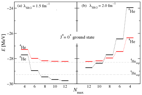
Figure 2: Dependence of the NCSM ⁶He and ⁴He $J^{\pi}=0^{+}$ ground state energies $E$(g.s.) on the HO model space size $N_{\rm max}$ for the SRG-N³LO $NN$ potential with (a) $\lambda_{\rm SRG}=1.5$ fm^-1 and $\hbar\Omega=14$ MeV, and (b) $\lambda_{\rm SRG}=2.0$ fm^-1 and $\hbar\Omega=20$ MeV.

III.1 ⁴He and ⁶He square integrable eigenstates

Table 1: Energy ($E_{x}$) of the first 9 positive-parity states with $J\leq 2$ for ⁶He calculated within the NCSM for a model space of $N_{\mbox{max}}$=12.

$J^{\pi}$	$\lambda_{\rm SRG}=1.5$ fm-1	$\lambda_{\rm SRG}=2.0$ fm-1
0+	$-29.75$	$-28.72$
	$-22.73$	$-20.10$
	$-20.46$	$-15.25$
	$-19.04$	$-13.39$
1+	$-24.25$	$-22.28$
	$-18.77$	$-13.57$
2+	$-27.40$	$-26.24$
	$-24.78$	$-22.99$
	$-19.22$	$-13.84$

Table 2: Energy ($E_{x}$) of the first 6 negative-parity states with $J\leq 2$ for ⁶He calculated within the NCSM for a model space of $N_{\mbox{max}}$=13.

$J^{\pi}$	$\lambda_{\rm SRG}=1.5$ fm-1	$\lambda_{\rm SRG}=2.0$ fm-1
0-	$-21.40$	$-17.84$
1-	$-23.84$	$-20.97$
	$-21.63$	$-17.98$
	$-19.90$	$-16.12$
2-	$-23.33$	$-20.45$
	$-19.67$	$-15.96$

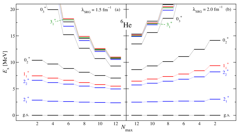
Figure 3: Dependence of the NCSM ⁶He $J^{\pi}=0^{+}$ excitation energies ($E_{\rm x}$) on the HO model space size $N_{\rm max}$ for the SRG-N³LO $NN$ potential with (a) $\lambda_{\rm SRG}=1.5$ fm^-1 and $\hbar\Omega=14$ MeV, and (b) $\lambda_{\rm SRG}=2.0$ fm^-1 and $\hbar\Omega=20$ MeV.

In this section, we discuss our results for the NCSM eigenstates used as input for the present NCSMC investigation of the $J^{\pi}=0^{+}$ g.s. of ⁶He and low-lying $\alpha$+$n$+$n$ continuum for partial waves up to $J^{\pi}=2^{\pm}$.

The computed energy of the ⁶He g.s. within the NCSM is presented in Fig. 2 as a function of the HO basis size $N_{\rm max}$. Results obtained with $\lambda_{\rm SRG}=1.5$ fm^-1 and $\hbar\Omega=14$ MeV, shown in panel (a), are compared with those in panel (b) for $\lambda_{\rm SRG}=2.0$ fm^-1 and $\hbar\Omega=20$ MeV. For the softer ($\lambda_{\rm SRG}=1.5$ fm^-1) potential, the variational NCSM calculations converge rapidly and can be easily extrapolated to $N_{\rm max}\rightarrow\infty$ using an exponential function of the type

$$E(N_{\rm max})=E_{\infty}+ae^{-bN_{\rm max}}.$$ (72)

This yields $E$(g.s.)$=-29.84(4)$ Quaglioni et al. (2013), which is about 0.6 MeV overbound with respect to experiment. The convergence rate is clearly slower for the $\lambda_{\rm SRG}=2.0$ fm^-1 interaction. Nevertheless, also in this case, the infinite-space g.s. energy can be accurately obtained using the extrapolation techniques recently developed for the NCSM Coon et al. (2012); Furnstahl et al. (2012); More et al. (2013); Furnstahl et al. (2014); Wendt et al. (2015). This was recently demonstrated by Sääf and Forssén, who obtained the extrapolated value of $E$(g.s.)$=-29.20(11)$ MeV Sääf and Forssén (2014) in close agreement with experiment (-29.268 MeV). Also shown in Fig. 2 are the corresponding results for the energy of the ⁴He g.s., which is used to build the microscopic cluster states of Eq. (2). For both $\lambda_{\rm SRG}$ values convergence is achieved within the largest HO model space, yielding binding energies close to experiment, as was already shown in Ref. Jurgenson et al. (2011).

Figure 3 shows the convergence pattern with respect to the HO basis size of the excitation energies for the first 10 positive-parity NCSM eigenstates of ⁶He. These include four 0⁺ , two 1⁺ and three 2⁺ states, and one $3^{+}$ state. This latter state is not used in the present NCSMC calculations. As before, the results obtained with the $\lambda_{\rm SRG}=1.5$ and $2.0$ fm^-1 interactions are shown in panel (a) and (b), respectively. Except for the $2^{+}_{1}$ state, which presents a very mild $N_{\rm max}$ dependence, the convergence rate is steady but slow, and tends to deteriorate as the excitation energy increases. The convergence rate is once again much faster for the softer potential, which also generates a more compressed excitation spectrum compared to the $\lambda_{\rm SRG}=2.0$ fm^-1 interaction. The overall picture is similar for the negative-parity states. A summary of the NCSM eigenenergies used as input in the largest model space adopted is given in Tables 1 and 2 for positive and negative parities, respectively.

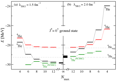
Figure 4: Same as Fig. 2 including also the dependence of the NCSMC ⁶He $J^{\pi}=0^{+}$ ground state energy ($E$) on the HO model space size $N_{\rm max}$ for the SRG-evolved N³LO $NN$ potential with (a) $\lambda_{\rm SRG}=1.5$ fm^-1 and $\hbar\Omega=14$ MeV, and (b) $\lambda_{\rm SRG}=2.0$ fm^-1 and $\hbar\Omega=20$ MeV. The extrapolated $N_{\rm max}\to\infty$ NCSM ⁶He is shown as a band of which the width represents the extrapolation uncertainty.

Table 3: Computed ⁶He g.s. energies (in MeV) within the cluster basis [⁴He(g.s.)+$n$+$n$] Quaglioni et al. (2013) ($4^{\rm th}$ column), NCSM ($5^{\rm th}$ column) and NCSMC including $N_{\lambda}=1$ eigenstate of the composite system ($6^{\rm th}$ column) as a function of the HO model space size $N_{\rm max}$ for the SRG-evolved N³LO $NN$ potential with $\lambda_{\rm SRG}=1.5$ fm^-1. Also shown for the biggest model space are the results for the NCSMC including $N_{\lambda}=4$ ⁶He eigenstates, and the NCSM ⁶He energy obtained through the exponential fit from Eq. (72). Results for ⁴He and experimental values for ⁶He are presented in the $3^{\rm rd}$ and last column, respectively.

$N_{\rm max}$	($N_{\lambda}$)	4He NCSM	6He Quaglioni et al. (2013)	6He NCSM	6He NCSMC	6He Expt.
6	(1)	$-27.98$	$-28.91$	$-28.95$	$-30.02$
8	(1)	$-28.17$	$-28.62$	$-29.45$	$-29.69$
10	(1)	$-28.21$	$-28.72$	$-29.66$	$-29.86$
12	(1)	$-28.22$	$-28.70$	$-29.75$	$-29.86$	$-29.268$ Brodeur et al. (2012)
12	(4)	–	–	–	$-29.88$
14	–	$-28.22$	–	–	–
$\infty$	–	–	–	$-29.84(4)$	–

III.2 ⁶He ground state within the NCSMC

Table 4: Same as Table 3, now using the potential obtained with a SRG evolution parameter of $\lambda=$2.0 fm^-1. The NCSM extrapolation shown is the one from Ref. Sääf and Forssén (2014). Note that for this potential the cluster basis alone does not yield a bound ⁶He ground state.

$N_{\rm max}$	($N_{\lambda}$)	4He NCSM	6He NCSM	6He NCSMC
6	(1)	$-27.44$	$-26.44$	$-28.31$
8	(1)	$-27.95$	$-27.70$	$-28.81$
10	(1)	$-28.18$	$-28.37$	$-28.97$
12	(1)	$-28.23$	$-28.72$	$-29.17$
12	(4)	–	–	$-29.17$
14	–	$-28.24$	–	–
$\infty$	–	–	$-29.20(11)$Sääf and Forssén (2014)
6He Expt.		$-29.268$ Brodeur et al. (2012)

The convergence of the ⁶He g.s. energy computed within the NCSMC in terms of the size of the model space is compared with the corresponding NCSM results in Fig. 4. More detailed comparisons (including with the results obtained working in a cluster basis alone Quaglioni et al. (2013)) are presented in Tables 3 and 4 for the $\lambda_{\rm SRG}=1.5$ fm^-1 and $\lambda_{\rm SRG}=2.0$ fm^-1 interactions, respectively. The $3^{\rm rd}$ column of Table 3 shows the energy of the ground state of ⁴He within the NCSM, which defines the three-body breakup energy threshold $E_{th}(\alpha+n+n)$ for all present ⁶He calculations. This is clearly already converged at the largest adopted model space size. The next three columns show the energy of the g.s. of ⁶He calculated within the ⁴He(g.s.)+$n$+$n$ cluster basis of Ref. Quaglioni et al. (2013), the NCSM and NCSMC. We can see that the fastest convergence is reached within the NCSMC. Furthermore, while the results from Ref. Quaglioni et al. (2013) also present a weak dependence on the HO model space size, they do not converge to the correct energy, which can be estimated by extrapolating to the infinity model space the NCSM results. This proves that the many-body correlations disregarded when using the cluster basis alone are indeed necessary for the correct description of the system and are correctly taken into account within the NCSMC. While the convergence of the NCSMC ⁶He g.s. energy with respect to the model space size is shown here for the case in which only one eigenstate of the composite system is included in the calculations, we also present the result obtained by including four eigenstates of ⁶He for the largest model space size. This shows that the inclusion of additional eigenstates of the composite system has only a small effect on the g.s. energy.

It is worth noting that the NCSMC is a variational approach as long as the adopted model space captures in full the wave function of the clusters (here, the ⁴He core) and of the aggregate system (here, ⁶He) or, equivalently, if it includes all possible pre-diagonalized eigenvectors of the clusters and of the aggregate system within the chosen $N_{\rm max}$ HO basis size. That is, the NCSMC is a variational approach as long as the generalized cluster expansion is not truncated. Such a model space is computationally unachievable and, for p-shell nuclei, we truncate the generalized cluster expansion to include only a few eigenstates of the cluster and aggregate nuclei. In particular, in the present application we only include the g.s. of the ⁴He core. The effect of this truncation manifest itself in the smallest HO base sizes, and can give rise to the non-variational behavior shown in Table 3 (the same argument applies to the cluster basis calculation of Ref. Quaglioni et al. (2013)). However, as the adopted HO basis size increases, thanks to the overcomplete nature of the NCSMC basis the wave functions of clusters and aggregate system are better and better represented within the truncated cluster expansion and the convergence behavior becomes variational, with the typical approach to the g.s. energy from above.

In Ref. Romero-Redondo et al. (2016) the equivalent results were presented in terms of the absolute HO model space size $N_{\rm tot}=N_{0}+N_{\rm max}$, where $N_{0}$ is the number of quanta shared by the nucleons in their lowest configuration. However, given that the input for the NCSMC includes the elements of the composite and cluster bases at the same $N_{\rm max}$, we came to the conclusion that a comparison in terms of $N_{\rm max}$ provides a better picture of the relevance of each component in the full calculation. We also note that the last three columns of Table I in Ref. Romero-Redondo et al. (2016) present a mismatch with respect to the model space size reported in the first column, showing results obtained with an $N_{\rm{max}}$ value larger by 2 units. Therefore, we call the reader to consider the present tables to be the accurate representation of the results.

Table 5: Percentage of the norm of the ⁶He g.s. wave function that comes directly from the NCSM part of the basis ($\sum_{\lambda}c_{\lambda}^{2}$).

$N_{\rm max}$	$\lambda_{\mbox{\scriptsize{SRG}}}=$1.5 fm-1	$\lambda_{\mbox{\scriptsize{SRG}}}=$2.0 fm-1
8	$78\%$	—
10	$88\%$	$71\%$
12	$91\%$	$76\%$

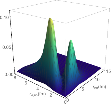
Figure 5: (Color online) Probability distribution the $J^{\pi}=0^{+}$ ground state of the ⁶He. Here $r_{nn}=\sqrt{2}\,\eta_{nn}$ and $r_{\alpha,nn}=\sqrt{3/4}\,\eta_{\alpha,nn}$ are, respectively, the distance between the two neutrons and the distance between the c.m. of ⁴He and that of the two neutrons.

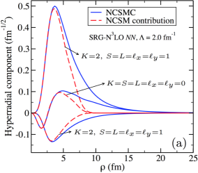
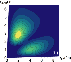
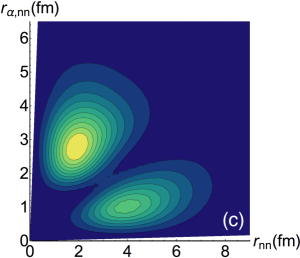
Figure 6: (Color online) Panel (a): Most relevant hyperradial components $\tilde{u}_{\nu K}(\rho)$ [see text] of the $\alpha$+$n$+$n$ relative motion within the ⁶He g.s. after projection of the $\lambda=2.0$ fm^-1 full NCSMC wave function in the largest model space (blue solid lines) as well as of its NCSM portion (red dashed lines) into the orthogonalized microscopic-cluster basis. Panel (b) and (c): Contour plots of the probability distribution obtained from the projection of the full NCSMC wave function of panel (a) and its NCSM component, respectively, as a function of the relative coordinates $r_{nn}=\sqrt{2}\,\eta_{nn}$ and $r_{\alpha,nn}=\sqrt{3/4}\,\eta_{\alpha,nn}$.

As seen in Table 4, convergence is not as obviously reached when using the harder potentials with $\lambda_{\mbox{\scriptsize{SRG}}}=2.0$ fm^-1. Within the NCSMC, there still are 200 keV difference between the $N_{\rm max}$= 10 and 12 results. However, the fact that the value obtained for $N_{\rm max}$= 12 (-29.17 MeV) is in agreement with the NCSM extrapolation from Ref. Sääf and Forssén (2014) (-29.20(11)) is a good indicator that our results are at least very close to convergence at this model space size.

We can estimate how much of the wave function can be described through the NCSM by calculating the percentage of the norm that comes directly from the discrete part of the basis, i.e. $\sum_{\lambda}c_{\lambda}^{2}$. These percentages are shown in Table 5 for the two different potentials used, as well as for different sizes of the model space. We find that, as one would expect, the NCSM component of the basis is able to describe a much larger percentage of the wave function when using the softer potential corresponding to the $\lambda_{\rm{SRG}}=1.5$ fm^-1 resolution scale, and also a larger and larger percentage as the HO model space size increases.

III.2.1 Spatial distribution

In Fig. 5 we show the probability density, as defined in section II.5, for the ground state of ⁶He in terms of the the distance between the two halo neutrons ($r_{nn}=\sqrt{2}\,\eta_{nn}$) and the distance between the ⁴He $core$ and the center of mass of the external neutrons ($r_{\alpha,nn}=\sqrt{3/4}\,\eta_{\alpha,nn}$). This density plot presents two peaks, which correspond to the two preferred spatial configurations of the system. The di-neutron configuration, which corresponds to the two neutrons being close together, clearly presents a higher probability respect to the cigar configuration in which the two neutrons are far apart and at the opposite sides of the $core$. This distribution is in agreement with previous studies Descouvemont et al. (2003); Brida and Nunes (2010); Quaglioni et al. (2013); Kukulin et al. (1986); Zhukov et al. (1993); Sääf and Forssén (2014); Nielsen et al. (2001). In order to estimate the reliability of the approximation of Eq. (68), which uses the projection of the NCSMC wave function into the cluster basis, we integrated the probability density given by Eq. (68). This integral is equivalent to the square of the norm of the projected wave function. We obtained 0.971 for the potential with $\lambda_{\rm SRG}=1.5$ fm^-1 and 0.967 for the potential with $\lambda_{\rm SRG}=2.0$ fm^-1. Given that we work with normalized wave functions, the proximity of these integrals to the unity indicates that only a small part of the wave functions was lost when performing the projection.

Table 6: Computed ⁴He and ⁶He matter radii (in fm) for $\lambda_{\rm{SRG}}=1.5$ fm^-1 and $\lambda_{\rm{SRG}}=2.0$ fm^-1 as a function of the HO model space size $N_{\rm max}$ within the NCSM, and the NCSMC including $N_{\lambda}=1$ eigenstates of the composite system. Also shown for the biggest model space are the results for the NCSMC including $N_{\lambda}=4$ ⁶He eigenstates. Experimental values for ⁶He are presented in the last column.

			$\lambda_{\rm SRG}=1.5$ fm-1				$\lambda_{\rm SRG}=2.0$ fm-1				Expt.
$N_{\rm max}$	($N_{\lambda}$)		4He NCSM	6He NCSM	6He NCSMC		4He NCSM	6He NCSM	6He NCSMC		6He
6	(1)		1.489	$2.14$	$2.47$		1.471	$2.01$	$2.47$
8	(1)		1.490	$2.18$	$2.35$		1.461	$2.06$	$2.40$		2.33(4)Tanihata et al. (1992)
10	(1)		1.487	$2.22$	$2.38$		1.461	$2.10$	$2.42$		2.30(7)Alkhazov et al. (1997)
12	(1)		1.490	$2.25$	$2.37$		1.459	$2.15$	$2.41$		2.37(5)Kiselev et al. (2005)
12	(4)		–	–	–		–	–	2.46(2)

Table 7: Computed ⁴He and ⁶He point-proton radii (in fm) for $\lambda_{\rm{SRG}}=1.5$ fm^-1 and $\lambda_{\rm{SRG}}=2.0$ fm^-1 as a function of the HO model space size $N_{\rm max}$ within the NCSM, and the NCSMC including $N_{\lambda}=1$ eigenstates of the composite system. Also shown for the biggest model space are the results for the NCSMC including $N_{\lambda}=4$ ⁶He eigenstates. Experimental values for ⁶He are presented in the last column.

			$\lambda_{\rm SRG}=1.5$ fm-1				$\lambda_{\rm SRG}=2.0$ fm-1				Expt.
$N_{\rm max}$	($N_{\lambda}$)		4He NCSM	6He NCSM	6He NCSMC		4He NCSM	6He NCSM	6He NCSMC		6He
6	(1)		1.501	$1.75$	$1.92$		1.474	$1.68$	$1.91$
8	(1)		1.493	$1.77$	$1.85$		1.464	$1.70$	$1.86$
10	(1)		1.490	$1.78$	$1.86$		1.464	$1.72$	$1.89$		1.938(23) Bacca et al. (2012)
12	(1)		1.487	$1.79$	$1.85$		1.462	$1.74$	$1.87$
12	(4)		–	–	–		–	–	1.90(2)

When the ⁶He ground state wave function is calculated within the NCSM basis, the probability density can be obtained by projecting into a cluster basis in the same way as it is done for the NCSMC in Eq. (65). The obtained projected wave function presents the same distribution observed in the case of the NCSMC, with the difference that it is less extended. This picture is consistent with the results previously reported in Ref. Sääf and Forssén (2014), and is to be expected given that within this basis the three-body asymptotic behavior is not well described. This is easily appreciated in Fig. 6, where the contour diagram of the probability distribution is shown for the NCSMC in panel (b) and for the NCSM component in panel (c). In the contour plots, it is also easier to determine the position on the probability maxima: within the di-neutron configuration the highest probability density appears when the neutrons are about 2 fm apart and the ⁴He $core$ about 3 fm from them. Within the cigar configuration, the neutrons are about 4 fm apart and the $core$ around 1 fm from their center of mass.

In panel (a) of Fig. 6, the most relevant hyperradial components $\tilde{u}_{\nu K}(\rho)$ of the $\alpha$+$n$+$n$ relative motion are shown. The hyperradial components $\tilde{u}_{\nu K}(\rho)$ are analogous to ${u}_{\nu K}(\rho)$ from Eq. (52) but defined for the projected wave function from Eq. (65). The solid blue lines are the components from the full NCSMC wave function while the dashed red lines represent the contribution to the full NCSMC wave function coming from the discrete NCSM eigenstates. This figures also provides a good visualization of how the short range of the NCSM wave function is complemented with the cluster basis to reproduce the extended wave function typical of halo nuclei by means of the NCSMC.

III.2.2 Radii

The spatial extension of a particular state can be estimated by its matter radius as described in section II.6. In table 6, we show the calculated NCSMC rms matter radius for the ground state of ⁶He as a function of the HO model space size $N_{\rm max}$. Results are shown for both $\lambda_{\rm SRG}=1.5$ fm^-1 and $\lambda_{\rm SRG}=2.0$ fm^-1. The results obtained within the NCSM alone are also shown for comparison. The introduction of ⁴He(g.s.)+$n$+$n$ microscopic cluster basis states provides a matter radius closer to experiment within smaller model spaces. Contrary to the NCSM, the convergence of the radius with respect to the size of the model space is achieved within the NCSMC at computationally accessible model spaces. The importance of the inclusion of the cluster states is even more pronounced for the potential with $\lambda_{\rm SRG}$=2.0 fm^-1, for which the NCSM results are further away from convergence. Similar to the g.s. energy discussed earlier, here too the convergence of the NCSMC is studied for the case in which only one eigenstate of the composite system is included in the calculation. In the largest HO model space, the inclusion of 3 additional (4 total) square-integrable eigenstates of the ⁶He system, yields a 2% increase of the matter radius. Besides the contributions coming from the rms matter radii of the additional discrete basis states, which are largely suppressed by the fact that the corresponding expansion coefficients ($c_{\lambda}$) are small, such an increase comes from the matrix elements of the matter radius operator between the first and third $0^{+}$ square integrable basis states. Our most complete results of $2.46(2)$ fm lies just above the range of experimental matter radii spanned by the values and associated error bars of Refs. Tanihata et al. (1992); Alkhazov et al. (1997); Kiselev et al. (2005) of $2.33(10)$.

Table 7 presents analogous results for the point-proton radius. Convergence behavior and comparisons with the NCSM are also analogous. Even though the protons belong to the core and not to the halo, the extension of the halo plays an important role for the point-proton radius. It displaces the center of mass of the core from the center of mass of the whole system, increasing the point-proton radius as it is easily seen in Eq. (71). Our most complete results of $1.90(2)$ fm is on the lower side but compatible with the bounds for the point-proton radius [$1.938(23)$ fm] as evaluated in Ref. Bacca et al. (2012).

It is important to point out that while the use of the $\lambda_{\rm SRG}$=1.5 fm^-1 SRG parameter produces a softer $NN$ potential and hence faster convergence, it is known that at this resolution scale there are significant SRG-induced $3N$ forces as well as SRG-induced two- and three-body contributions to the radii. Within the present calculations we are disregarding such induced terms. Therefore, the results obtained with this resolution scale are expected to be far from realistic and they should be understood as an instrument to study the NCSMC approach rather than as realistic predictions for the ⁶He nucleus.

A summary of the rms radii obtained for the more realistic $\lambda_{\rm SRG}$=2.0 fm^-1 interaction is presented in Table 8 and visualized in Fig. 7 together with the corresponding results for the separation energy, the infinite-basis extrapolations from Ref. Sääf and Forssén (2014), and the effective interaction hyperspherical harmonics (EIHH) calculations from Ref. Bacca et al. (2012), based on the $V_{{\rm low}k}$(N³LO) $NN$ interaction at the resolution scales $\Lambda_{{\rm low}k}=1.8$, and 2.0 fm^-1. (The results presented Table 8 have been obtained with improved accuracy and supersede those shown in Table II of Ref. Romero-Redondo et al. (2016), where the labeling of the HO model space size was also incorrectly reported to be lower by two units.)

Table 8: Summary of the results presented in Fig. 7, with $\Lambda_{{\rm low}k}$ in units of fm^-1. See text for further details.

		$S_{2n}$ (MeV)	$r_{m}$ (fm)	$r_{pp}$ (fm)
NCSM	($N_{\rm max}=12$)	0.49	2.15	1.74
NCSM Sääf and Forssén (2014)	($N_{\rm max}=\infty$)	0.95(10)	–	1.820(4)
NCSMC	($N_{\rm max}=12$)	0.94(5)	2.46(2)	1.90(2)
EIHH Bacca et al. (2012)	($\Lambda_{{\rm low}k}=1.8$)	1.036(7)	2.30(6)	1.78(1)
EIHH Bacca et al. (2012)	($\Lambda_{{\rm low}k}=2.0$)	0.82(4)	2.33(5)	1.804(9)
Expt.		0.975	2.33(10)	1.938(23)

The two-nucleon separation energy obtained within the NCSMC is close to its empirical value, and the computed $r_{m}$ and $r_{pp}$ radii are, respectively, at the upper end of and on the lower side but compatible with their experimental bands. Interestingly, our point-proton radius is substantially larger than both the extrapolated value of Sääf et al., which “calls for further investigations” Sääf and Forssén (2014), and the EIHH result of Bacca et al. Bacca et al. (2012). This latter calculation also yields a matter radius smaller than ours though within the experimental bounds. The present combination of $S_{2n}$ and $r_{pp}$ values are more in line with the Green’s function Monte Carlo results of Ref. Pieper (2008), based on $NN$+$3N$ forces constrained to reproduce the properties of light nuclei including ⁶He.

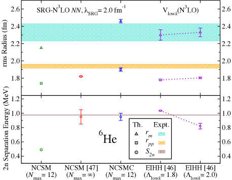
Figure 7: (Color online) NCSM (green symbols) and NCSMC (blue symbols) rms matter (triangles) and point-proton (squares) radii, and two-neutron separation energy (circles), obtained using the SRG-N³LO $NN$ interaction with $\lambda_{\rm SRG}=2.0$ fm^-1 in the largest HO model space. Also shown are the infinite-basis extrapolations from Ref. Sääf and Forssén (2014) (red symbols) and the EIHH results from Ref. Bacca et al. (2012) (indigo symbols) at the resolution scales $\Lambda_{{\rm low}k}=1.8$, and 2.0 fm^-1. The range of experimental values are represented by horizontal bands (see text for more details).

III.3 ⁴He+$n$+$n$ continuum

We investigated the low-lying $\alpha$+$n$+$n$ continuum for partial waves up to $J^{\pi}$ = 2^± by solving the set of Eqs. (55) with the boundary conditions from Eq. (63). The eigenphase shifts were extracted from the diagonalization of the three-body scattering matrix $S_{\nu K,\nu^{\prime}K^{\prime}}$.

Convergence of the results with respect to the HO model-space size and the parameters used to perform the matching between the solutions in the internal region and the asymptotic wave functions within the $R$-matrix approach was reached at similar values as those used in our previous study of Ref. Romero-Redondo et al. (2014), lacking the contribution from square-integrable eigenstates of the composite system. Specifically, our best results were obtained at $N_{\mbox{max}}$=12, which is the maximum computationally accessible HO model space size, and interested readers can find a complete list of the remaining parameters for each channel in Appendix D.

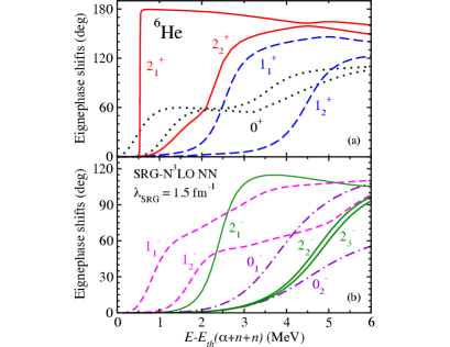
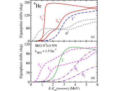
Figure 8: Attractive eigenphase shifts below 6 MeV above the two-neutron emission threshold [$E_{th}$($\alpha$+$n$+$n$)] computed within the NCSMC [panels (a) and (b)] and within the more limited model space spanned by the ⁴He(g.s.)+$n$+$n$ cluster basis alone of Ref. Romero-Redondo et al. (2014) [panels (c) and (d)], using the SRG-evolved N³LO $NN$ potential with $\lambda_{\rm SRG}=$ 1.5 fm^-1. We show positive parity states in panels (a) and (c), and negative parity states in panels (b) and (d).

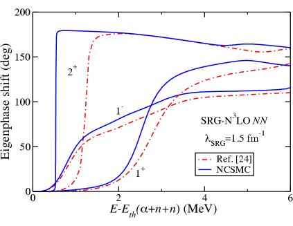
Figure 9: Eigenphase shifts for the $J^{\pi}=1^{\pm}$ and 2⁺ channels computed within the NCSMC (blue solid line) and within the more limited model space spanned by the ⁴He(g.s.)+$n$+$n$ cluster basis alone of Ref. Romero-Redondo et al. (2014) (red dot-dashed line) using the SRG-evolved N³LO $NN$ potential with $\lambda_{\rm SRG}=$ 1.5 fm^-1.

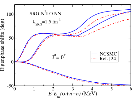
Figure 10: Eigenphase shifts for the $J^{\pi}$= 0⁺ channel computed within the NCSMC (blue solid line) and within the more limited model space spanned by the ⁴He(g.s.)+$n$+$n$ cluster basis alone of Ref. Romero-Redondo et al. (2014) (red dot-dashed line) using the SRG-evolved N³LO $NN$ potential with $\lambda_{\rm SRG}=$ 1.5 fm^-1.

In Fig. 8(a) and (b), we present a summary of the most relevant attractive eigenphase shifts below $6$ MeV obtained for the $\lambda_{\rm SRG}=$ 1.5 fm^-1 interaction within the NCSMC by including the first nine positive-parity and six negative-parity $J\leq 2$ square-integrable eigenstates of the composite system. This figure can be compared with Fig. 1 of Ref. Romero-Redondo et al. (2014) – for convenience shown again in Fig. 8(c) and (d) – which presents analogous results computed within the more limited model space spanned by the ⁴He(g.s.)+$n$+$n$ cluster basis alone. Although the qualitative behavior of the eigenphase shifts is similar, within the NCSMC the centroid values of all resonances tend to be shifted to lower energies and the resonance widths tend to shrink due to the effect of the inclusion of discrete eigenstates of the composite system. The most significant change is observed for the first 2⁺ resonance, which becomes much sharper (with a width of $\Gamma=15$ keV) and is shifted to lower energies (with the new centroid at 0.536 MeV). This behavior suggests a likely significant influence of the chiral 3N force on this state. The effect in other partial waves is more modest. In particular, the $1^{-}$ eigenphase shift does not change significantly, excluding core-polarization effects as the possible origin of a low-lying soft dipole mode. This can more readily be observed in Fig. 9 and 10, where we show a direct comparison between the present results and those of Ref. Romero-Redondo et al. (2014) for the lowest resonances in the 1^± and 2⁺ channels and for the lowest three eigenphase shifts in the 0⁺ channel, respectively. The repulsive eigenphase shift in the 0⁺ channel corresponds to the ground state of ⁶He, and the small difference between the calculations is related to the difference in the binding energy, as it was shown in Table 3.

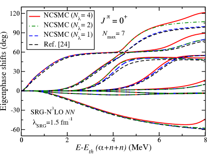
Figure 11: Convergence with respect to the number ($N_{\lambda}$) of square-integrable eigenstates of the composite system included in the NCSMC calculation of the eigenphase shifts for the 0⁺ channel, using the SRG-evolved N³LO $NN$ potential with $\lambda_{\rm SRG}=$ 1.5 fm^-1. Also shown are the results from Ref. Romero-Redondo et al. (2014), corresponding to the inclusion of zero composite states (cluster basis alone).

The convergence of the eigenphase shifts with respect to the number of eigenstates of the composite system included in the calculation was found to be very fast. The mere inclusion of the lowest eigenstate is in general sufficient to obtain reasonable convergence in the low-energy region. As an example, we show in Fig. 11 the convergence pattern of the $J^{\pi}=0^{+}$ eigenphase shifts with respect to the number of NCSM eigenstates of the composite system for a small model space of size $N_{\rm max}$= 7. Two eigenstates are already sufficient for obtaining convergence up to 5 MeV. For energies below 3 MeV, a single eigenstate is enough. This convergence behavior is of course related to the value of the eigenenergies associated with the included square-integrable eigenstates. The further the eigenvalue is from the energy under consideration, the smaller the contribution to the eigenphase shifts from the corresponding eigenstate. (The eigenenergies of all positive- and negative-parity eigenstates included in the $N_{\rm max}=12$ calculations are shown in tables 1 and 2, respectively.) For comparison, the eigenphase shifts of Ref. Romero-Redondo et al. (2014), calculated within the cluster basis alone, are also shown (corresponding to zero eigenstates included).

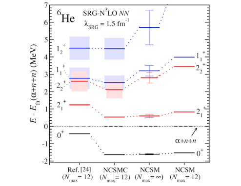
Figure 12: Spectrum of low-lying energy levels of the ⁶He nucleus for $\lambda_{\rm SRG}=1.5$ as obtained within the ⁴He(g.s.)+$n$+$n$ cluster basis of Ref. Romero-Redondo et al. (2014), the NCSMC, and within the NCSM by treating the ⁶He excited states as bound states. For the NCSM , we show both the energy levels at $N_{\rm max}$=12 and the results of an extrapolation to the infinite model space, performed through the exponential fit function from Eq. (72).

From the calculated eigenphase shifts, it is possible to extract information about the resonances by calculating the centroids $E_{R}$ and widths $\Gamma$ as the values of $E_{\rm kin}=E-E_{th(\alpha+n+n)}$ for which the first derivative $\delta^{\prime}(E_{kin})$ of the eigenphase shifts is maximal and $\Gamma{=}2/\delta^{\prime}(E_{R})$, respectively Thompson and Nunes (2009). The resulting low-lying ⁶He spectrum of energy levels for the SRG-evolved N³LO $NN$ interaction with $\lambda_{\rm SRG}=1.5$ fm^-1 is shown in Fig. 12. There, we compare the present NCSMC results with the spectra computed within the cluster basis alone Romero-Redondo et al. (2014), and within the NCSM (i.e., by treating the ⁶He excited states as bound states). Besides the results at $N_{\rm max}=12$, for the NCSM we also show the spectrum obtained by extrapolation to the infinite HO model space using the exponential form of Eq. (72). Note that, while for the results of Ref. Romero-Redondo et al. (2014) and the NCSMC the resonances are represented by their centroids (solid line) and width (shaded area), for the NCSM we only show the energy levels and associate estimated uncertainty of the extrapolation. Indeed, such a bound-state technique does not yield resonance widths. While broad, higher-energy states such as the 1${}^{+}_{2}$ resonance are well described already within a ⁴He(g.s)+$n$+$n$ picture and very narrow resonances such as the first 2⁺ can already be explained within the bound-state approximations of the NCSM, for other intermediate levels both short-range many-body correlations and continuum degrees of freedom play an important role.

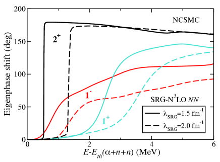
Figure 13: Eigenphase shifts for the$J^{\pi}=1^{\pm}$ and 2⁺ channels computed within the NCSMC using the SRG-evolved N³LO $NN$ potential with $\lambda_{\rm SRG}=$ 1.5 fm^-1 (solid lines) and $\lambda_{\rm SRG}=$ 2.0 fm^-1 (dashed lines).

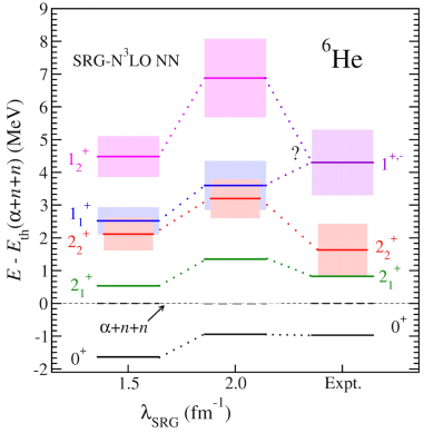
Figure 14: Spectra of low-lying energy levels of the ⁶He nucleus computed within the NCSMC using the SRG-evolved N³LO $NN$ potential with $\lambda_{\rm SRG}=$ 1.5 fm^-1 and $\lambda_{\rm SRG}=$ 2.0 fm^-1 compared to the most recent experimental spectrum of Ref. Mougeot et al. (2012).

The harder $NN$ interaction obtained with the SRG resolution scale of $\lambda=2.0$ fm^-1 produces a qualitatively similar picture, but with higher-lying and wider resonances. This is highlighted in Figs. 13 and 14, showing respectively the eigenphase shifts for the $J^{\pi}=1^{\pm}$ and 2⁺ channels, and a comparison of the computed energy levels with the most recent experimental spectrum of Ref. Mougeot et al. (2012). The observed dependence on the value of the SRG resolution scale provides an estimate of the effect of induced $3N$ (and higher order) forces, which have been disregarded in the present study and are crucial to restore the formal unitarity of the adopted SRG transformation of the Hamiltonian. More in general, the inclusion of 3N forces (including the initial chiral $3N$ force) is indispensable to arrive at an accurate description of the spectrum as a whole. Indeed, while the SRG-evolved $NN$ interaction with $\lambda=2.0$ fm^-1 provides a realistic description of the energy and structure of the ⁶He ground state, neither of the two adopted resolution scales describes accurately the spectrum of the low-energy excited states. At the same time, based on these results we conjecture that the parity of the $J=1$ resonance populated at SPIRAL through the ⁸He($p,^{3}$He)⁶He* two-neutron transfer reaction Mougeot et al. (2012) is likely positive, making it less probable that this state is the soft-dipole mode called for by Refs. Nakayama et al. (2000) and Nakamura et al. (2000).

IV Conclusions

We presented the extension of the ab initio no-core shell model with continuum to the treatment of bound and continuum nuclear systems in the proximity of a three-body breakup threshold. This approach takes simultaneously into account both many-body short-range correlations and clustering degrees of freedom, allowing for a comprehensive ab initio description of nuclear systems presenting a three-cluster configuration such as Borromean halo nuclei and light-nuclei reactions with three nuclear fragments in either entrance or exit channels.

After introducing the NCSMC ansatz for systems characterized by a three-cluster asymptotic behavior, we discussed the dynamical equations, and gave the algebraic expressions of the overlap and Hamiltonian couplings between the discrete and continuous NCSMC basis states for the particular case of core+$n$+$n$ systems. Further, we discussed the procedure adopted for the solution of the three-cluster dynamical equations for bound and scattering states, and explained how we calculate the probability density, and the matter and point-proton root-mean-square radii starting from the obtained NCSMC solutions for core+$n$+$n$ systems. The new formalism was then applied to conduct a comprehensive study of many-body correlations and $\alpha$-clustering in the ground-state and low-lying energy continuum of the Borromean ⁶He nucleus using the chiral N³LO $NN$ potential or Ref. Entem and Machleidt (2003) softened via the similarity renormalization group method Bogner et al. (2007); Roth et al. (2008); Wegner (1994).

Calculations were carried out using a soft ($\lambda_{\rm SRG}=1.5$ fm^-1) SRG resolution scale to allow for a direct comparison with the results obtained in the more limited studies of Refs. Quaglioni et al. (2013); Romero-Redondo et al. (2014), based solely on the three-cluster portion of the NCSMC basis. While working within the ⁴He(g.s.)+$n$+$n$ microscopic cluster basis it is possible to reproduce the correct asymptotic behavior of the ⁶He wave function, we demonstrated that additional short-range six-body correlations (included in the form of square-integrable eigenstates of the composite ⁶He system) are necessary to correctly describe also the interior of the wave function for both the ground and scattering states. In particular, a significant portion of the ground-sate energy and the narrow width of the first 2⁺ resonance stem from many-body correlations that, in a microscopic-cluster picture, can be interpreted as core-excitation effects.

A second and physically more interesting potential ($\lambda_{\rm SRG}=2.0$ fm^-1) was also used. Though the inclusion of $3N$ forces (currently underway) remains crucial to restore the formal unitarity of the adopted SRG transformation of the Hamiltonian and arrive at an accurate description of the spectrum as a whole, the present results demonstrated that rms matter and point-proton radii compatible with experiment can be obtained starting from a soft $NN$ interaction reprodu cing the ⁶He small binding energy.

In the future we plan to reexamine the ab initio calculation of the ⁶He $\beta$-decay half-life, first carried out in Ref. Schiavilla and Wiringa (2002), in the context of chiral effective field theory using wave functions with proper asymptotic behavior. This work also sets the stage for the ab initio study of the ⁴He$(2n,\gamma)^{6}$He radiative capture and is a stepping stone in the calculation of the ³H$(^{3}{\rm H},2n)^{4}$He fusion.

Appendix A Norm and Hamiltonian kernels

Here we present the explicit expressions for the NCSMC Hamiltonian and norm kernels entering Eqs. (II.4) and (48). There, the square and inverse-square root of the NCSMC norm kernel, ${\mathbb{N}}^{\pm\frac{1}{2}}$, can be written as

$$({\mathbb{N}}^{\pm\frac{1}{2}})^{\lambda\lambda^{\prime}}_{\nu xy,\nu^{\prime}x^{\prime}y^{\prime}} =\left(\begin{array}[]{ccc}0&&0\\[5.69054pt] 0&&\delta_{\nu\nu^{\prime}}\frac{\delta(x-x^{\prime})}{xx^{\prime}}\frac{\delta(y-y^{\prime})}{yy^{\prime}}-\delta_{\nu\nu^{\prime}}\delta_{n^{\prime}_{x}n_{x}}\delta_{n^{\prime}_{y}n_{y}}R_{n_{x}\ell_{x}}(x)R_{n_{x}\ell_{x}}(x^{\prime})R_{n_{y}\ell_{y}}(y)R_{n_{y}\ell_{y}}(y^{\prime})\\[5.69054pt] \end{array}\right)$$ (75)

$$+\left(\begin{array}[]{ccc}\delta_{\lambda\tilde{\lambda}}&&0\\[5.69054pt] 0&&R_{n_{x}\ell_{x}}(x)R_{n_{y}\ell_{y}}(y)\delta_{\nu\tilde{\nu}}\end{array}\right)({\mathbb{N}}^{\pm\frac{1}{2}})^{\tilde{\lambda}\tilde{\lambda}^{\prime}}_{\tilde{\nu}n_{x}n_{y},\tilde{\nu}^{\prime}n_{x}^{\prime}n_{y}^{\prime}}\left(\begin{array}[]{ccc}\delta_{\tilde{\lambda}^{\prime}\lambda^{\prime}}&&0\\[5.69054pt] 0&&R_{n_{x}^{\prime}\ell_{x}^{\prime}}(x^{\prime})R_{n_{y}^{\prime}\ell_{y}^{\prime}}(y^{\prime})\delta_{\tilde{\nu}^{\prime}\nu^{\prime}}\end{array}\right),$$ (80)

where the sum over the repeating indexes $\tilde{\lambda},\tilde{\nu},n_{x},n_{y},\tilde{\lambda}^{\prime},\tilde{\nu}^{\prime},n_{x}^{\prime}$, and $n_{y}^{\prime}$ is implied, and the notation

$$({\mathbb{N}}^{\pm\frac{1}{2}})^{\lambda\lambda^{\prime}}_{\nu n_{x}n_{y},\nu^{\prime}n_{x}^{\prime}n_{y}^{\prime}}=\left(\begin{array}[]{ccc}({\mathbb{N}}^{\pm\frac{1}{2}})^{(11)}_{\lambda\lambda^{\prime}}&&({\mathbb{N}}^{\pm\frac{1}{2}})^{(12)}_{\lambda\nu^{\prime}n_{x}^{\prime}n_{y}^{\prime}}\\[5.69054pt] ({\mathbb{N}}^{\pm\frac{1}{2}})^{(21)}_{\lambda^{\prime}\nu n_{x}n_{y}}&&({\mathbb{N}}^{\pm\frac{1}{2}})^{(22)}_{\nu n_{x}n_{y},\nu^{\prime}n_{x}^{\prime}n_{y}^{\prime}}\end{array}\right)$$ (83)

stands for the matrix elements of the square and inverse-square root of the NCSMC norm kernel within the model space, which are computed from the NCSMC model-space norm kernel

$${\mathbb{N}}^{\lambda\lambda^{\prime}}_{\nu n_{x}n_{y},\nu^{\prime}n_{x}^{\prime}n_{y}^{\prime}}=\left(\begin{array}[]{ccc}\delta_{\lambda\lambda^{\prime}}&&\bar{g}_{\lambda\nu^{\prime}n_{x}^{\prime}n_{y}^{\prime}}\\[5.69054pt] \bar{g}_{\lambda^{\prime}\nu n_{x}n_{y}}&&\delta_{\nu\nu^{\prime}}\delta_{n_{x}n_{x}^{\prime}}\delta_{n_{y}n_{y}^{\prime}}\end{array}\right)$$ (86)

using the spectral theorem. The orthogonalized Hamiltonian within the model space can then be calculated as follows

$$\overline{\mathbb{H}}^{\lambda\lambda^{\prime}}_{\nu n_{x}n_{y},\nu^{\prime}n_{x}^{\prime}n_{y}^{\prime}}=\left(\begin{array}[]{ccc}\overline{\mathbb{H}}^{(11)}_{\lambda\lambda^{\prime}}&&\overline{\mathbb{H}}^{(12)}_{\lambda\nu^{\prime}n_{x}^{\prime}n_{y}^{\prime}}\\ \overline{\mathbb{H}}^{(21)}_{\lambda^{\prime}\nu n_{x}n_{y}}&&\overline{\mathbb{H}}^{(22)}_{\nu n_{x}n_{y},\nu^{\prime}n_{x}^{\prime}n_{y}^{\prime}}\end{array}\right)=({\mathbb{N}}^{-\frac{1}{2}})^{\lambda\tilde{\lambda}}_{\nu n_{x}n_{y},\tilde{\nu}\tilde{n}_{x}\tilde{n}_{y}}{\mathbb{H}}^{\tilde{\lambda}\tilde{\lambda}^{\prime}}_{\tilde{\nu}\tilde{n}_{x}\tilde{n}_{y},\tilde{\nu}^{\prime}\tilde{n}_{x}^{\prime}\tilde{n}_{y}^{\prime}}({\mathbb{N}}^{-\frac{1}{2}})^{\tilde{\lambda}^{\prime}\lambda^{\prime}}_{\tilde{\nu}^{\prime}\tilde{n}_{x}^{\prime}\tilde{n}_{y}^{\prime},\nu^{\prime}n_{x}^{\prime}n_{y}^{\prime}},$$ (87)

where the sum over the repeating indexes $\tilde{\lambda},\tilde{\nu},\tilde{n}_{x},\tilde{n}_{y},\tilde{\lambda}^{\prime},\tilde{\nu}^{\prime},\tilde{n}_{x}^{\prime}$, and $\tilde{n}_{y}^{\prime}$ is, once again, implied, and

$${\mathbb{H}}^{\lambda\lambda^{\prime}}_{\nu n_{x}n_{y},\nu^{\prime}n_{x}^{\prime}n_{y}^{\prime}}=\left(\begin{array}[]{lcl}E_{\lambda}\delta_{\lambda\lambda^{\prime}}&&\bar{h}_{\lambda\nu^{\prime}n_{x}^{\prime}n_{y}^{\prime}}\\[5.69054pt] \bar{h}_{\lambda^{\prime}\nu n_{x}n_{y}}&&\overline{\mathcal{H}}_{\nu n_{x}n_{y},\nu^{\prime}n_{x}\ n_{y}^{\prime}}\end{array}\right)\,,$$ (90)

is the model-space component of the NCSMC Hamiltonian kernel of Eq. (8). We note that the coupling form factors in configuration space, $\bar{h}_{\lambda\nu}(x,y)=[h{\mathcal{N}}^{-\frac{1}{2}}]_{\lambda\nu}(x,y)$ are related to those in the model space, $\bar{h}_{\lambda\nu n_{x}n_{y}}$, through Eqs. (15) and (36), and the lower-diagonal block is the model-space component of the orthonormalized integration kernel of Eq. (12). Additional details on how this kernel is computed can be found in Ref. Quaglioni et al. (2013), where we introduced the formalism for the description of three-cluster dynamics based solely on expansions over three-cluster channels states of the type of Eq. (2).

Finally, in the following we provide detailed expressions for the blocks forming the orthogonalized NCSMC Hamiltonian of Eq. (II.4), including the terms that extend beyond the HO model space $P$. In particular, in the following we will use the notation $n\in P$ to indicate that the radial quantum number $n\leq N_{\rm max}$. Note that for the upper diagonal bock there are not additional terms that reach beyond the the HO model space and, therefore, it is trivially given by the upper diagonal block of Eq. (87).

$$\overline{\mathbb{H}}^{(12)}_{\lambda\nu^{\prime}}(x^{\prime},y^{\prime})=\sum_{n_{x}^{\prime}n_{y}^{\prime}}R_{n_{x}^{\prime}\ell_{x}^{\prime}}(x^{\prime})R_{n_{y}^{\prime}\ell_{y}^{\prime}}(y^{\prime})\overline{\mathbb{H}}^{(12)}_{\lambda\nu^{\prime}n_{x}^{\prime}n_{y}^{\prime}}$$

$$\qquad+\sum_{\tilde{\lambda}}({\mathbb{N}}^{-\frac{1}{2}})^{(11)}_{\lambda\tilde{\lambda}}\left[\sum_{n_{y}^{\prime}\in P}R_{N+1\ell_{x}^{\prime}}(x^{\prime})g_{\tilde{\lambda}\nu^{\prime}Nn_{y}^{\prime}}T^{\ell_{x}^{\prime}}_{NN+1}R_{n_{y}^{\prime}\ell_{y}^{\prime}}(y^{\prime})+\sum_{n_{x}^{\prime}\in P}R_{N+1\ell_{y}^{\prime}}(y^{\prime})g_{\tilde{\lambda}\nu^{\prime}n_{x}^{\prime}N}T^{\ell_{y}^{\prime}}_{NN+1}R_{n_{x}^{\prime}\ell_{x}^{\prime}}(x^{\prime})\right]$$

$$\qquad+\sum_{\tilde{\nu}}\sum_{\tilde{n}_{x}\tilde{n}_{y}n_{y}^{\prime}\in P}({\mathbb{N}}^{-\frac{1}{2}})^{(12)}_{\lambda\tilde{\nu}\tilde{n}_{x}\tilde{n}_{y}}\left(\frac{1}{2}\Lambda^{-\frac{1}{2}}_{\tilde{\nu}\tilde{n}_{x}\tilde{n}_{y},\nu^{\prime}Nn_{y}^{\prime}}+\frac{1}{2}\Lambda^{\frac{1}{2}}_{\tilde{\nu}\tilde{n}_{x}\tilde{n}_{y},\nu^{\prime}Nn_{y}^{\prime}}\right)T^{\ell_{x}^{\prime}}_{NN+1}R_{N+1\ell_{x}^{\prime}}(x^{\prime})R_{n_{y}^{\prime}\ell_{y}^{\prime}}(y^{\prime})$$

$$\qquad+\sum_{\tilde{\nu}}\sum_{\tilde{n}_{x}\tilde{n}_{y}n_{x}^{\prime}\in P}({\mathbb{N}}^{-\frac{1}{2}})^{(12)}_{\lambda\tilde{\nu}\tilde{n}_{x}\tilde{n}_{y}}\left(\frac{1}{2}\Lambda^{-\frac{1}{2}}_{\tilde{\nu}\tilde{n}_{x}\tilde{n}_{y},\nu^{\prime}n_{x}^{\prime}N}+\frac{1}{2}\Lambda^{\frac{1}{2}}_{\tilde{\nu}\tilde{n}_{x}\tilde{n}_{y},\nu^{\prime}n_{x}^{\prime}N}\right)T^{\ell_{y}^{\prime}}_{NN+1}R_{N+1\ell_{y}^{\prime}}(y^{\prime})R_{n_{x}^{\prime}\ell_{x}^{\prime}}(x^{\prime})\,,$$ (91)

$$\overline{\mathbb{H}}^{(21)}_{\lambda^{\prime}\nu}(x,y)=\sum_{n_{x}n_{y}}R_{n_{x}\ell_{x}}(x)R_{n_{y}\ell_{y}}(y)\overline{\mathbb{H}}^{(21)}_{\lambda^{\prime}\nu n_{x}n_{y}}$$

$$\qquad+\sum_{\tilde{\lambda}}\left[\sum_{n_{y}\in P}R_{N+1\ell_{x}}(x)g_{\tilde{\lambda}\nu Nn_{y}}T^{\ell_{x}}_{NN+1}R_{n_{y}\ell_{y}}(y)+\sum_{n_{x}\in P}R_{N+1\ell_{y}}(y)g_{\tilde{\lambda}\nu n_{x}N}T^{\ell_{y}}_{NN+1}R_{n_{x}\ell_{x}}(x)\right]({\mathbb{N}}^{-\frac{1}{2}})^{(11)}_{\tilde{\lambda}\lambda^{\prime}}$$

$$\qquad+\sum_{\tilde{\nu}}\sum_{\tilde{n}_{x}\tilde{n}_{y}n_{y}\in P}R_{N+1\ell_{x}}(x)R_{n_{y}\ell_{y}}(y)T^{\ell_{x}}_{N+1N}\left(\frac{1}{2}\Lambda^{-\frac{1}{2}}_{\nu Nn_{y},\tilde{\nu}\tilde{n}_{x}\tilde{n}_{y}}+\frac{1}{2}\Lambda^{\frac{1}{2}}_{\nu Nn_{y},\tilde{\nu}\tilde{n}_{x}\tilde{n}_{y}}\right)({\mathbb{N}}^{-\frac{1}{2}})^{(21)}_{\lambda^{\prime}\tilde{\nu}\tilde{n}_{x}\tilde{n}_{y}}$$

$$\qquad+\sum_{\tilde{\nu}}\sum_{\tilde{n}_{x}\tilde{n}_{y}n_{x}\in P}R_{n_{x}\ell_{x}}(x)R_{N+1\ell_{y}}(y)T^{\ell_{y}}_{N+1N}\left(\frac{1}{2}\Lambda^{-\frac{1}{2}}_{\nu n_{x}N,\tilde{\nu}\tilde{n}_{x}\tilde{n}_{y}}+\frac{1}{2}\Lambda^{\frac{1}{2}}_{\nu n_{x}N,\tilde{\nu}\tilde{n}_{x}\tilde{n}_{y}}\right)({\mathbb{N}}^{-\frac{1}{2}})^{(21)}_{\lambda^{\prime}\tilde{\nu}\tilde{n}_{x}\tilde{n}_{y}}\,,$$ (92)

and

$$\overline{\mathbb{H}}^{(22)}_{\nu\nu^{\prime}}(x,y,x^{\prime},y^{\prime})=\frac{\delta(y-y^{\prime})}{yy^{\prime}}\delta_{\nu\nu^{\prime}}T_{\nu}(x)\frac{\delta(x-x^{\prime})}{xx^{\prime}}+\frac{\delta(x-x^{\prime})}{xx^{\prime}}\delta_{\nu\nu^{\prime}}T_{\nu}(y)\frac{\delta(y-y^{\prime})}{yy^{\prime}}$$

$$\qquad-\delta_{\nu\nu^{\prime}}\left[\sum_{n_{y}\in P}\left(R_{N+1\ell_{x}}(x)T^{\ell_{x}}_{N+1N}R_{N\ell_{x}}(x^{\prime})+R_{N\ell_{x}}(x)T^{\ell_{x}}_{NN+1}R_{N+1\ell_{x}}(x^{\prime})\right)R_{n_{y}\ell_{y}}(y)R_{n_{y}\ell_{y}}(y^{\prime})\right.$$

$$\qquad+\sum_{n_{x}\in P}R_{n_{x}\ell_{x}}(x)R_{n_{x}\ell_{x}}(x^{\prime})\left(R_{N+1\ell_{y}}(y)T^{\ell_{y}}_{N+1N}R_{N\ell_{y}}(y^{\prime})+R_{N\ell_{y}}(y)T^{\ell_{y}}_{NN+1}R_{N+1\ell_{y}}(y^{\prime})\right)$$

$$\qquad+\sum_{n_{x}n_{y}n_{x}^{\prime}\in P}R_{n_{x}\ell_{x}}(x)T^{\ell_{x}}_{n_{x}n_{x}^{\prime}}R_{n_{x}^{\prime}\ell_{x}^{\prime}}(x^{\prime})R_{n_{y}\ell_{y}}(y)R_{n_{y}\ell_{y}^{\prime}}(y^{\prime})$$

$$\qquad+\left.\sum_{n_{x}n_{y}n_{y}^{\prime}\in P}R_{n_{x}\ell_{x}}(x^{\prime})R_{n_{x}\ell_{x}^{\prime}}(x^{\prime})R_{n_{y}\ell_{y}}(y)T^{\ell_{y}}_{n_{y}n_{y}^{\prime}}R_{n_{y}^{\prime}\ell_{y}^{\prime}}(y^{\prime})\right]$$

$$\qquad+\sum_{n_{x}n_{y}n_{x}^{\prime}n_{y}^{\prime}}R_{n_{x}^{\prime}\ell_{x}^{\prime}}(x^{\prime})R_{n_{y}^{\prime}\ell_{y}^{\prime}}(y^{\prime})R_{n_{x}\ell_{x}}(x)R_{n_{y}\ell_{y}}(y)\overline{\mathbb{H}}^{(22)}_{\nu n_{x}n_{y}\nu^{\prime}n_{x}^{\prime}n_{y}^{\prime}}$$

$$\qquad+\sum_{\tilde{\lambda}}\left[\sum_{n_{y}\in P}R_{N+1\ell_{x}}(x)g_{\tilde{\lambda}\nu Nn_{y}}T^{\ell_{x}}_{NN+1}R_{n_{y}\ell_{y}}(y)+\sum_{n_{x}\in P}R_{N+1\ell_{y}}(y)g_{\tilde{\lambda}\nu n_{x}N}T^{\ell_{y}}_{NN+1}R_{n_{x}\ell_{x}}(x)\right]$$

$$\qquad\times\sum_{n_{x}^{\prime}n_{y}^{\prime}\in P}R_{n_{x}^{\prime}\ell_{x}^{\prime}}(x^{\prime})R_{n_{y}^{\prime}\ell_{y}^{\prime}}(y^{\prime})({\mathbb{N}}^{-\frac{1}{2}})^{(12)}_{\tilde{\lambda}\nu^{\prime}n_{x}^{\prime}n_{y}^{\prime}}$$

$$\qquad+\sum_{\tilde{\nu}}\sum_{\begin{subarray}{c}\tilde{n}_{x}\tilde{n}_{y}\\ n_{y}n_{x}^{\prime}\\ n_{y}^{\prime}\in P\end{subarray}}R_{N+1\ell_{x}}(x)R_{n_{y}\ell_{y}}(y)T^{\ell_{x}}_{N+1N}\left(\frac{1}{2}\Lambda^{-\frac{1}{2}}_{\nu Nn_{y},\tilde{\nu}\tilde{n}_{x}\tilde{n}_{y}}+\frac{1}{2}\Lambda^{\frac{1}{2}}_{\nu Nn_{y},\tilde{\nu}\tilde{n}_{x}\tilde{n}_{y}}\right)({\mathbb{N}}^{-\frac{1}{2}})^{(22)}_{\tilde{\nu}\tilde{n}_{x}\tilde{n}_{y},\nu^{\prime}n_{x}^{\prime}n_{y}^{\prime}}R_{n_{x}^{\prime}\ell_{x}^{\prime}}(x^{\prime})R_{n_{y}^{\prime}\ell_{y}^{\prime}}(y^{\prime})$$

$$\qquad+\sum_{\tilde{\nu}}\sum_{\begin{subarray}{c}\tilde{n}_{x}\tilde{n}_{y}\\ n_{x}^{\prime}n_{y}^{\prime}\\ n_{x}\in P\end{subarray}}R_{n_{x}\ell_{x}}(x)R_{N+1\ell_{y}}(y)T^{\ell_{y}}_{N+1N}\left(\frac{1}{2}\Lambda^{-\frac{1}{2}}_{\nu n_{x}N,\tilde{\nu}\tilde{n}_{x}\tilde{n}_{y}}+\frac{1}{2}\Lambda^{\frac{1}{2}}_{\nu n_{x}N,\tilde{\nu}\tilde{n}_{x}\tilde{n}_{y}}\right)({\mathbb{N}}^{-\frac{1}{2}})^{(22)}_{\tilde{\nu}\tilde{n}_{x}\tilde{n}_{y}\nu^{\prime}n_{x}^{\prime}n_{y}^{\prime}}R_{n_{x}^{\prime}\ell_{x}^{\prime}}(x^{\prime})R_{n_{y}^{\prime}\ell_{y}^{\prime}}(y^{\prime})$$

$$\qquad+\sum_{\tilde{\lambda}}\sum_{n_{x}n_{y}}({\mathbb{N}}^{-\frac{1}{2}})^{(21)}_{\tilde{\lambda}\nu n_{x}n_{y}}R_{n_{x}\ell_{x}}(x)R_{n_{y}\ell_{y}}(y)$$

$$\qquad\times\left[\sum_{n_{y}^{\prime}\in P}R_{N+1\ell_{x}^{\prime}}(x^{\prime})g_{\tilde{\lambda}\nu^{\prime}Nn_{y}^{\prime}}T^{\ell_{x}^{\prime}}_{NN+1}R_{n_{y}^{\prime}\ell_{y}^{\prime}}(y^{\prime})+\sum_{n_{x}^{\prime}\in P}R_{N+1\ell_{y}^{\prime}}(y^{\prime})g_{\tilde{\lambda}\nu^{\prime}n_{x}^{\prime}N}T^{\ell_{y}^{\prime}}_{NN+1}R_{n_{x}^{\prime}\ell_{x}^{\prime}}(x^{\prime})\right]$$

$$\qquad+\sum_{\tilde{\nu}}\sum_{\begin{subarray}{c}\tilde{n}_{x}\tilde{n}_{y}\\ n_{x}n_{y}\\ n_{y}^{\prime}\in P\end{subarray}}R_{n_{x}\ell_{x}}(x)R_{n_{y}\ell_{y}}(y)({\mathbb{N}}^{-\frac{1}{2}})^{(22)}_{\nu n_{x}n_{y},\tilde{\nu}\tilde{n}_{x}\tilde{n}_{y}}\left(\frac{1}{2}\Lambda^{-\frac{1}{2}}_{\tilde{\nu}\tilde{n}_{x}\tilde{n}_{y},\nu^{\prime}Nn_{y}^{\prime}}+\frac{1}{2}\Lambda^{\frac{1}{2}}_{\tilde{\nu}\tilde{n}_{x}\tilde{n}_{y},\nu^{\prime}Nn_{y}^{\prime}}\right)T^{\ell_{x}^{\prime}}_{NN+1}R_{N+1\ell_{x}^{\prime}}(x^{\prime})R_{n_{y}^{\prime}\ell_{y}^{\prime}}(y^{\prime})$$

$$\qquad+\sum_{\tilde{\nu}}\sum_{\begin{subarray}{c}\tilde{n}_{x}\tilde{n}_{y}\\ n_{x}n_{y}\\ n_{x}^{\prime}\in P\end{subarray}}R_{n_{x}\ell_{x}}(x)R_{n_{y}\ell_{y}}(y)({\mathbb{N}}^{-\frac{1}{2}})^{(22)}_{\nu n_{y}n_{y},\tilde{\nu}\tilde{n}_{x}\tilde{n}_{y}}\left(\frac{1}{2}\Lambda^{-\frac{1}{2}}_{\tilde{\nu}\tilde{n}_{x}\tilde{n}_{y},\nu^{\prime}n_{x}^{\prime}N}+\frac{1}{2}\Lambda^{\frac{1}{2}}_{\tilde{\nu}\tilde{n}_{x}\tilde{n}_{y},\nu^{\prime}n_{x}^{\prime}N}\right)T^{\ell_{y}^{\prime}}_{NN+1}R_{N+1\ell_{y}^{\prime}}(y^{\prime})R_{n_{x}^{\prime}\ell_{x}^{\prime}}(x^{\prime})\,,$$ (93)

where the subindex $N$ is the maximum size of the HO model space, which has been referred to as $N_{\rm max}$ throughout the paper, $T^{\ell}_{nn^{\prime}}=\langle n\ell|\hat{T}_{rel}|n^{\prime}\ell\rangle$ are matrix elements of the relative kinetic energy operator, and $\Lambda$ represents the model-space norm kernel within the more limited formalism for the description of three-cluster dynamics based solely on expansions over three-cluster channels states of the type of Eq. (2) (see Eqs. (A3) - (A6) of Ref. Quaglioni et al. (2013)).

Appendix B Wave functions

As described in section II.4, instead of solving directly Eq. (5) we solve the set of orthogonalized Schrödinger equations Eq. (II.4). Therefore, we obtain the orthogonalized vector of the expansion coefficients $\overline{\mathbb{C}}^{\lambda}_{\nu xy}$ instead of the original ${\mathbb{C}}^{\lambda}_{\nu xy}$. These two arrays are related through Eq. (48), which can be inverted into

$${\mathbb{C}}^{\lambda}_{\nu xy} =\left[{\mathbb{N}}^{-\frac{1}{2}}\overline{\mathbb{C}}\right]^{\lambda}_{\nu xy}=\left(\begin{array}[]{c}{c}_{\lambda}\\ \chi_{\nu}(x,y)\end{array}\right)\,.$$ (96)

Therefore, we can recover the original ${\mathbb{C}}^{\lambda}_{\nu xy}$ through the following expressions:

$${c}_{\lambda} = \sum_{\lambda^{\prime}}({\mathbb{N}}^{-\frac{1}{2}})^{(11)}_{\lambda\lambda^{\prime}}\overline{c}_{\lambda^{\prime}}+\sum_{\nu}\iint dxx^{2}dyy^{2}({\mathbb{N}}^{-\frac{1}{2}})^{(12)}_{\lambda\nu xy}\overline{\chi}_{\nu}(xy)$$

$$\chi_{\nu}(xy) = \sum_{\lambda}({\mathbb{N}}^{-\frac{1}{2}})^{(21)}_{\lambda\nu xy}\overline{c}_{\lambda}+\sum_{\nu^{\prime}}\iint dx^{\prime}x^{\prime 2}dy^{\prime}y^{\prime 2}({\mathbb{N}}^{-\frac{1}{2}})^{(22)}_{\nu xy\nu^{\prime}x^{\prime}y^{\prime}}\overline{\chi}_{\nu^{\prime}}(x^{\prime}y^{\prime})\,.$$ (97)

Appendix C Radii expressions

The expectation value for the radii operators within the NCSMC wave function can be expressed in terms of the cluster and composite bases as

$$\langle\Psi^{J^{\pi}T}|\hat{r}^{2}|\Psi^{J^{\pi}T}\rangle =\sum_{\lambda\lambda^{\prime}}c_{\lambda}c_{\lambda^{\prime}}\langle A\lambda J^{\pi}T|\hat{r}^{2}|A\lambda^{\prime}J^{\pi}T\rangle$$

$$+\sum_{\lambda\nu^{\prime}}c_{\lambda}\int dx^{\prime}dy^{\prime}x^{\prime 2}y^{\prime 2}G_{\nu^{\prime}}^{J^{\pi}T}(x^{\prime},y^{\prime})\langle\phi_{\nu^{\prime}x^{\prime}y^{\prime}}^{J^{\pi}T}|\hat{A}_{\nu^{\prime}}\hat{r}^{2}|A\lambda J^{\pi}T\rangle$$

$$+\sum_{\lambda^{\prime}\nu}c_{\lambda^{\prime}}\int dxdyx^{2}y^{2}G_{\nu}^{J^{\pi}T}(x,y)\langle A\lambda^{\prime}J^{\pi}T|\hat{r}^{2}\hat{A}_{\nu}|\phi_{\nu xy}^{J^{\pi}T}\rangle$$

$$+\sum_{\nu\nu^{\prime}}\iint dxdydx^{\prime}dy^{\prime}x^{2}y^{2}x^{\prime 2}y^{\prime 2}G_{\nu}^{J^{\pi}T}(x,y)G_{\nu^{\prime}}^{J^{\pi}T}(x^{\prime},y^{\prime})\langle\phi_{\nu^{\prime}x^{\prime}y^{\prime}}^{J^{\pi}T}|\hat{A}_{\nu^{\prime}}\hat{r}^{2}\hat{A}_{\nu}|\phi_{\nu xy}^{J^{\pi}T}\rangle,$$ (98)

where, $\hat{r}^{2}$ represents either the matter or point proton radii operators. The root mean square radii are given by the square root of these matrix elements. Note that in Eq. (C) the first term corresponds to the expectation value within a NCSM calculation weighted by the product of the discrete expansion amplitudes $c_{\lambda}$ and $c_{\lambda^{\prime}}$. This first term is calculated using the general expressions of the corresponding operators, however, the rest of the terms are calculated using the expressions that were derived in Sec. II.6 considering the clusterization of the system, i.e., Eq. (70) and the right side of Eq. (71) for the matter and point-proton radii, respectively. For the coupling terms, i.e., the second and third terms in Eq. (C), mixed matrix elements are needed. We calculate these matrix elements by expanding, in an approximate way, the NCSM state into the cluster basis. While this is in principle a rough approximation we can conclude a posteriori that the results are not significantly affected by this approximation given that the contribution of these coupling terms in this first order is already very small compared to the other terms.

When calculating the matter radius, Eq. (C) reduces to

$$\langle\Psi^{J^{\pi}T}|r_{m}^{2}|\Psi^{J^{\pi}T}\rangle=$$

$$\quad=\sum_{\lambda\lambda^{\prime}}c^{J^{\pi}T}_{\lambda}c^{J^{\pi}T}_{\lambda^{\prime}}\langle A\lambda J^{\pi}T|r_{m}^{2}|A\lambda^{\prime}J^{\pi}T\rangle$$

$$\quad+\left(\frac{A-2}{A}\right)\sum_{\nu\nu^{\prime}}\langle A-a_{23}\,\alpha_{1}I_{1}^{\pi_{1}}T_{1}|r_{m}^{2,{\rm core}}|A-a_{23}\,\alpha_{1}I_{1}^{\pi_{1}}T_{1}\rangle\iint dxdyx^{2}y^{2}W^{J^{\pi}T}_{\nu\nu^{\prime}}(x,y)$$

$$\quad+\frac{1}{A}\sum_{\nu\nu^{\prime}}\iint dxdyx^{2}y^{2}\rho^{2}W^{J^{\pi}T}_{\nu\nu^{\prime}}(x,y)\,.$$ (99)

For the point-proton radius, Eq. (71) is valid given that the $core$ is the only charged cluster and has isospin zero. The expectation value is given by

$$\langle\Psi^{J^{\pi}T}|r_{pp}^{2}|\Psi^{J^{\pi}T}\rangle=$$

$$\qquad=\sum_{\lambda}c^{J^{\pi}T}_{\lambda}c^{J^{\pi}T}_{\lambda^{\prime}}\langle A\lambda J^{\pi}T|r_{pp}^{2}|A\lambda^{\prime}J^{\pi}T\rangle$$

$$\qquad+\langle A-a_{23}\,\alpha_{1}I_{1}^{\pi_{1}}T_{1}|r_{pp}^{2,{\rm core}}|A-a_{23}\,\alpha_{1}I_{1}^{\pi_{1}}T_{1}\rangle\iint dxdyx^{2}y^{2}W^{J^{\pi}T}_{\nu\nu^{\prime}}(x,y)$$

$$\qquad+\sqrt{\frac{2}{A(A-2)}}\sum_{\nu\nu^{\prime}}\iint dxdyx^{2}y^{4}W^{J^{\pi}T}_{\nu\nu^{\prime}}(x,y)\,.$$ (100)

Here and in the equation above we have defined

$$W^{J^{\pi}T}_{\nu\nu^{\prime}}(x,y) =\frac{1}{2}G^{J^{\pi}T}_{\nu^{\prime}-}(x,y)G^{J^{\pi}T}_{\nu+}(x,y)+\frac{1}{2}G^{J^{\pi}T}_{\nu^{\prime}+}(x,y)G^{J^{\pi}T}_{\nu-}(x,y)$$

$$+\sum_{\lambda^{\prime}}c_{\lambda^{\prime}}^{J^{\pi}T}g^{J^{\pi}T}_{\lambda^{\prime}\nu^{\prime}}(x,y)G^{J^{\pi}T}_{\nu-}(x,y)+G^{J^{\pi}T}_{\nu^{\prime}-}(x,y)\sum_{\lambda}c_{\lambda}^{J^{\pi}T}g^{J^{\pi}T}_{\lambda\nu}(x,y),$$ (101)

with

$$G^{J^{\pi}T}_{\nu\pm}(x,y)=\sum_{\nu^{\prime}}\iint dx^{\prime}dy^{\prime}x^{\prime 2}y^{\prime 2}[\mathcal{N}^{J^{\pi}T}_{\nu\nu^{\prime}}(x,y,x^{\prime},y^{\prime})]^{\pm 1/2}\chi^{J^{\pi}T}_{\nu^{\prime}}(x^{\prime},y^{\prime}).$$ (102)

Appendix D Parameters of the calculations

For completeness, in Tables 9 and  10 we list all parameters besides the HO model space size ($N_{\rm max}=12$) used for our best calculations for each $J^{\pi}T$ channel.

Table 9: Parameters used for the calculations with $\lambda_{\rm{SRG}}$=1.5 fm^-1

$J^{\pi}$	$N_{\mbox{ext}}$	$K_{\mbox{max}}$	$a$ (fm)	$n_{s}$	$n_{\alpha}$
0+	200	40	45	125	40
0-	70	18	30	60	20
1+	70	19	30	60	30
1-	110	23	40	80	40
2+	90	20	30	60	40
2-	70	18	30	60	20

Table 10: Parameters used for the calculations with $\lambda_{\rm{SRG}}$=2.0 fm^-1

$J^{\pi}$	$N_{\mbox{ext}}$	$K_{\mbox{max}}$	$a$ (fm)	$n_{s}$	$n_{\alpha}$
0+	200	40	45	150	50
1+	110	23	40	95	45
1-	110	23	40	95	45
2+	90	20	30	60	40