Entrainment in the Master Equation

Abstract

The master equation plays an important role in many scientific fields including physics, chemistry, systems biology, physical finance, and sociodynamics. We consider the master equation with periodic transition rates. This may represent an external periodic excitation like the 24h solar day in biological systems or periodic traffic lights in a model of vehicular traffic. Using tools from systems and control theory, we prove that under mild technical conditions every solution of the master equation converges to a periodic solution with the same period as the rates. In other words, the master equation entrains (or phase locks) to periodic excitations. We describe two applications of our theoretical results to important models from statistical mechanics and epidemiology.

I Introduction

Consider a physical system that can be in one of exactly $N$ possible configurations: $C_{1},\dots,C_{N}$. Let $x_{i}(t)\in[0,1]$ denote the probability that the system is in configuration $i$ at time $t$. Let $x(t):=\begin{bmatrix}x_{1}(t)&\dots&x_{N}(t)\end{bmatrix}^{\prime}$ denote the (column) state-vector of probabilities at time $t$.

The master equation describes the time evolution of these probabilities:

$$\dot{x}_{1}(t) =\sum_{\genfrac{}{}{0.0pt}{}{j=1}{j\not=1}}^{N}p_{j1}(t,x(t))x_{j}(t)-\sum_{\genfrac{}{}{0.0pt}{}{j=1}{j\not=1}}^{N}p_{1j}(t,x(t))x_{1}(t),$$

$$\vdots$$

$$\dot{x}_{N}(t) =\sum_{\genfrac{}{}{0.0pt}{}{j=1}{j\not=N}}^{N}p_{jN}(t,x(t))x_{j}(t)-\sum_{\genfrac{}{}{0.0pt}{}{j=1}{j\not=N}}^{N}p_{Nj}(t,x(t))x_{N}(t),$$ (1)

where $p_{ji}(t,x(t))\geq 0$ denotes the rate of transition from configuration $C_{j}$ to configuration $C_{i}$. We assume a general case where the transition rates at time $t$ may depend on both $t$ and the state $x(t)$. This makes (I) a time-varying nonlinear dynamical system.

Define $H:\mathbb{R}^{N}\to\mathbb{R}$ by $H(y):=y_{1}+\dots+y_{N}$. Since $x_{i}$ represents the probability of being in configuration $C_{i}$, we assume that the initial condition $x(t_{0})$ satisfies $H(x(t_{0}))=x_{1}(t_{0})+\dots+x_{N}(t_{0})=1$. Eq. (I) then implies that

$$\sum_{i=1}^{N}\dot{x}_{i}(t)\equiv 0,$$ (2)

so $H(x(t,t_{0},x(t_{0})))\equiv 1$, that is, $H$ is a first integral of (I). This simply means that summing the probabilities of being at configuration $C_{i}$ over all possible $i$ yields one.

The master equation can be explained intuitively as describing the balance of probability currents going in and out of each possible state. A rigorous derivation for a chemically reacting gas-phase system that is kept well stirred and in thermal equilibrium is given in [1]. The master equation plays a fundamental role in physics (where it is sometimes referred to as the Pauli master equation), chemistry, systems biology, sociodynamics, and more. See e.g. the monographs [2, 3] for more details.

In the special case where $p_{ij}(t,x)=p_{ij}(t)$ for all $i$, $j$ system (I) is related to a Markov process in the following way. Denote by $P_{\tau}$ the fundamental matrix of (I) with $P_{\tau}(\tau)=I_{N}$. Then $P_{\tau}(t)$ is a stochastic matrix (i.e. the sum of every column of $P_{\tau}(t)$ is equal to one) for $t\geq\tau$. The obvious relation $P_{s}(t)P_{\tau}(s)=P_{\tau}(t)$ for $\tau<s<t$ encodes the Chapman-Kolmogorov equations if we interpret $(P_{\tau}(t))_{ij}$ as transition probabilities for a system to be in configuration $C_{i}$ at time $t$, provided it is in configuration $C_{j}$ at time $\tau$. Together with an initial probability distribution on the states $1,\ldots,N$, the transition probabilities then define a unique Markov process and equation (I) is called its forward equation [4, 5].

In many physical systems the number of possible configurations $N$ can be very large. For example, the well-known totally asymmetric simple exclusion principle TASEP model (see, e.g. [6, 7] and the references therein) includes a lattice of $n$ consecutive sites, and each site can be either free or occupied by a particle, so the number of possible configuration is $N=2^{n}$. In such cases, simulating the master equation and calculating its steady-state may be difficult and special methods must be applied (see, e.g. [8, 7]).

Here, we are interested in deriving theoretical results that hold for any $N$. Specifically, we consider the case where the transition rates are periodic with a common period $T>0$, that is,

$$p_{ij}(t+T,x)=p_{ij}(t,x),$$ (3)

for all $i,j$, all $t$, and all $x$. We refer to (I) with the rates satisfying (3) as the $T$-periodic master equation. Note that this includes the case where one [or several] of the rates is [are] $T$-periodic with $T>0$, and the other rates are time-independent, as a time-independent function satisfies (3) for all $T$. Clearly, from (3) it also follows that $p_{ij}(t+kT,x)=p_{ij}(t,x)$ for any integer $k$. In order to make the period a well defined notion one therefore often requires that the period is the minimal real number $T>0$ for which (3) is satisfied. Then constant functions do not have a period. Since we want to include here the case of time-independent transition rates, see e.g. Corollary 6 below, we do not require the minimality of the common period $T$ in (3).

We consider the problem of entrainment (or phase-locking) in the $T$-periodic master equation.

Problem 1.

Given a system described by a $T$-periodic master equation, determine if for every initial condition the probabilities $x_{i}(t)$, $i=1,\dots,N$, converge to a periodic solution with period $T$. If this is so, determine if the periodic solution is unique or not.

In other words, if we view the transition rates as a $T$-periodic excitation then the problem is to determine if the state of the system entrains, that is, converges to a periodic trajectory with the same period $T$. If this is so, an important question is whether there exist a unique periodic trajectory $\gamma$ and then every solution converges to $\gamma$.

Entrainment is important in many natural and artificial systems. For example, organisms are often exposed to periodic excitations like the 24h solar day and the periodic cell-cycle division process. Proper functioning often requires accurate entrainment of various biological processes to this excitation [9]. For example, cardiac arrhythmias is a heart disorder occurring when every other pulse generated by the sinoatrial node pacemaker is ineffective in driving the ventricular rhythm [10].

Epidemics of infectious diseases often correlate with seasonal changes and the required interventions, such as pulse vaccination, may also need to be periodic [11]. In mathematical population models, this means that the so called transmission parameter is periodic, with a period of one year, and entrainment means that the spread of epidemics converges to a periodic pattern with the same period. As another example, traffic flow is often controlled by periodically-varying traffic lights. In this context, entrainment means that the traffic flow converges to a periodic pattern with the same period as the traffic lights. This observation could be useful for the study of the green wave phenomenon [12]. Another example, from the field of power electronics, involves connecting a synchronous generator to the electric grid. The periodically-varying voltage in the grid may be interpreted as a periodic excitation to the generator, and proper functioning requires the generator to entrain to this excitation (see e.g. [13] and the references therein).

In the special case of time-invariant rates Problem 1 reduces to determining if every solution converges to a steady-state, and whether there exits a unique steady-state. Indeed, time-invariant rates are $T$-periodic for any $T>0$ and thus entrainment means convergence to a solution that is $T$-periodic for any $T>0$, i.e. a steady-state.

Since the $x_{i}$s represent probabilities,

$$x_{i}(t)\in[0,1]\text{ for all $i$ and }\sum_{j}x_{j}(t)=1$$ (4)

for all $t\geq t_{0}$. The structure of the master equation guarantees that if $x(t)$ satisfies (4) at time $t=t_{0}$ then (4) holds for all $t\geq t_{0}$ even when the $x_{i}$s are not necessarily linked to probabilities. Our results below hold of course in this case as well. The next example demonstrates such a case.

Example 2.

An important topic in sociodynamics is the formation of large cities due to population migration. Ref. [2, Chapter 8] considers a master equation describing the flow of individuals between $N$ settlements. The transition rates $p_{ij}$ in this model represent the probability per time unit that an individual living in settlement $i$ will migrate to settlement $j$. A mean-field approximation of this master equation yields a model in the form (I), where $x_{i}$ represents the average density at settlement $i$, and $p_{ij}=\exp((x_{j}-x_{i})k_{ij})$, with $k_{ij}>0$. This models the fact that the rate of transition from settlement $i$ to settlement $j$ increases when the population in settlement $j$ is larger than in $i$, i.e. the tendency of individuals to migrate to larger cities. Note that the rates here are state-dependent, but not time-dependent. However, it is natural to assume that migration decisions depend on the season. For example, the tendency to migrate to colder cities may decrease [increase] in the winter [summer]. This can be modeled by adding time-dependence, say, changing the scaling parameters $k_{ij}$ to functions $k_{ij}(t)$, that are periodic with a period of one year. Then the transition rates depend on both state and time, and are periodic.

For small values of $N$ it is sometimes possible to solve the master equation and then analyze entrainment directly. The next example demonstrates this.

Example 3.

Consider the master equation (I) with $N=2$ and continuous time- (but not state-) dependent rates, i.e. $p_{ij}=p_{ij}(t)\geq 0$. Then (I) can be written as

$$\begin{bmatrix}\dot{x}_{1}\\ \dot{x}_{2}\end{bmatrix}=\begin{bmatrix}-p_{12}&p_{21}\\ p_{12}&-p_{21}\end{bmatrix}\begin{bmatrix}{x}_{1}\\ {x}_{2}\end{bmatrix}.$$ (5)

Assume also that all the rates are periodic with period $T>0$. Using the fact that $x_{1}(t)+x_{2}(t)\equiv 1$ yields

$$\dot{x}_{1}(t)=p_{21}(t)-(p_{12}(t)+p_{21}(t))x_{1}(t).$$ (6)

Recall that $x_{1}(0),x_{2}(0)\in[0,1]$ with $x_{1}(0)+x_{2}(0)=1$. Eq. (6) implies that $x_{1}(t)\in[0,1]$ for all $t\geq 0$, and thus $x_{2}(t)\in[0,1]$ for all $t\geq 0$. Solving (6) yields

$$x_{1}(t) =\exp\left(-\int_{0}^{t}(p_{12}(s)+p_{21}(s))\mathop{}\!\mathrm{d}s\right)(x_{1}(0)+c(t)),$$ (7)

$$x_{2}(t) =1-x_{1}(t),$$

where $c(t):=\int_{0}^{t}p_{21}(\tau)\exp\left(\int_{0}^{\tau}(p_{12}(s)+p_{21}(s))\mathop{}\!\mathrm{d}s\right)\mathop{}\!\mathrm{d}\tau$. To analyze if every solution converges to a periodic solution we consider two cases.

Case 1: If $p_{12}(t)+p_{21}(t)\equiv 0$ then (7) yields $x(t)\equiv x(0)$, i.e. every point in the state-space is an equilibrium point. This means that every solution is a periodic solution with period $T$.

Case 2: Assume that there exists a time $t^{*}\in[0,T)$ such that $p_{12}(t^{*}){+}p_{21}(t^{*})>0$. (Note that by continuity this in fact holds on a time interval that includes $t^{*}$). The solution (7) is periodic with period $T$ if and only if $x_{1}(T)=x_{1}(0)$ i.e. if and only if

$$x_{1}(0)=\frac{\exp\left(-\int_{0}^{T}(p_{12}(s)+p_{21}(s))\mathop{}\!\mathrm{d}s\right)c(T)}{1-\exp\left(-\int_{0}^{T}(p_{12}(s)+p_{21}(s))\mathop{}\!\mathrm{d}s\right)}.$$ (8)

It is straightforward to show that the right-hand side in this equation is in $[0,1]$, so in this case there exists a unique periodic trajectory $\gamma(t)$, with $\gamma_{1}(0)$ equal to the expression in (8), and $\gamma_{2}(0)=1-\gamma_{1}(0)$. To determine if every trajectory converges to $\gamma$, let $z(t):=x(t)-\gamma(t)$. Then

$$\dot{z}_{1}=-(p_{12}+p_{21})z_{1},\quad z_{1}(0)=x_{1}(0)-\gamma_{1}(0).$$

Since $p_{12}(t){+}p_{21}(t)$ is positive on a time interval, and $T$-periodic, $z_{1}(t)$ converges to zero, and we conclude that any trajectory of the system converges to the unique periodic solution $\gamma$.

Of course, when $N>2$ and the rates depend on both $t$ and $x$ this type of explicit analysis is impossible, and the proof of entrainment requires a different approach.

In general, proving that a time-varying nonlinear dynamical system entrains to periodic excitations is non trivial. Rigorous proofs are known for two classes of dynamical systems: contractive systems, and monotone systems admitting a first integral.

A system is called contractive if any two trajectories approach one another at an exponential rate [14, 15]. Such systems entrain to periodic excitations [9, 16]. An important special case is asymptotically stable linear systems with an additive periodic input $u$, that is, systems in the form

$$\dot{x}=Ax+Bu,$$ (9)

with $x\in\mathbb{R}^{N}$, $A\in\mathbb{R}^{N\times N}$ a Hurwitz matrix, $u\in\mathbb{R}^{M}$, and $B\in\mathbb{R}^{N\times M}$. In this case $x(t)$ converges to a periodic solution $\gamma(t)$ and it is also possible to obtain a closed-form description of $\gamma$ using the transfer function of the linear system [17]. We note that even in the case that the $p_{ij}$s in (I) do not depend on $x$, i.e., when (I) is linear in $x$, the master equation is not of the form (9) because the periodic influence in (I) enters through the transition rates $p_{ij}$ and not through an additive input channel.

A system is called monotone if its flow preserves a partial order, induced by an appropriate cone $K$, between its initial conditions [18]. An important special case are cooperative systems for which the cone $K$ is the positive orthant. Cooperative systems that admit a first integral entrain to periodic excitations. It is interesting to note that proofs of this property often follow from contraction arguments [19].

The master equation (I) is in general not contractive, although as we will show in Theorem 20 below it is on the “verge of contraction” with respect to the $\ell_{1}$ vector norm (see [20] for some related considerations). However, (I) admits a first integral and is often a cooperative system (see Theorem 21 below). In particular, when the rates do not depend on the state, i.e. $p_{ij}=p_{ij}(t)$ then (I) is always cooperative.

Although entrainment has attracted enormous research attention, it seems that it has not been addressed before for the general case of systems modeled using a $T$-periodic master equation. Here we apply the theory of cooperative dynamical systems admitting a first integral to derive conditions guaranteeing that the answer to Problem 1 is affirmative. In Section III, we describe two applications of our approach to important systems from statistical physics. The first is the totally asymmetric simple exclusion process (TASEP). This model has been introduced in the context of bio-cellular processes [21], and has become the standard model for the flow of ribosomes along the mRNA molecule during translation [22, 23]. More generally, TASEP has become a paradigmatic model for the statistical mechanics of nonequilibrium systems [6, 7, 24]. It is in particular used to study the stochastic dynamics of interacting particle systems such as vehicular traffic [25].

The second application is to an important model from epidemiology called the stochastic susceptible-infected-susceptible (SIS) model.

The remainder of this paper is organized as follows. In the next section we state the exact mathematical formulation of the master equation that we assume throughout together with our main results Theorems 5 and 8. Section III describes the two applications to statistical physics and to epidemiology mentioned above. This is followed by a brief discussion of the significance of the results and an outlook on possible future directions of research. The Appendix includes all the proofs. These are based on known tools, yet we are able to use the special structure of the master equation to derive stronger results than those available in the literature on monotone dynamical systems.

II Main results

We begin by specifying the exact conditions on (I) that are assumed throughout. For any time $t$, $x(t)$ is an $N$-dimensional column vector that includes the probabilities of all $N$ possible configurations. The relevant state-space is thus

$$\Omega:=\{y\in\mathbb{R}^{N}\,|\,y_{i}\geq 0\text{ for all }i,\text{ and }\sum_{i=1}^{N}y_{i}=1\}.$$

For an initial time $t_{0}\geq 0$ and an initial condition $x(t_{0})$, let $x(t;t_{0},x(t_{0}))$ denote the solution of (I) at time $t\geq t_{0}$. For our purposes it will be convenient to assume that the vector field associated with system (I) is not only defined on the set $\Omega$, but on all the closed positive cone

$$\mathbb{R}^{N}_{+}:=\{x\in\mathbb{R}^{N}\,|\,x_{j}\geq 0\mbox{ for all }1\leq j\leq N\}\,.$$

Throughout this paper we assume that the following condition holds.

Assumption 4.

There exists $T>0$ such that the transition rates $p_{ij}(t,{x})$ are: continuous and non-negative on $[0,T)\times\mathbb{R}^{N}_{+}$; continuously differentiable with respect to ${x}$ on $[0,T)\times\operatorname{{\mathrm{i}nt}}(\mathbb{R}^{N}_{+})$ and the derivative admits a continuous extension onto $[0,T)\times\mathbb{R}^{N}_{+}$; and are jointly periodic with period $T$, that is,

$$p_{ij}(t+T,{x})=p_{ij}(t,{x}),$$ (10)

for all $i,j$, all $t\in[0,T)$, and all ${x}\in\mathbb{R}^{N}_{+}$.

Let $\operatorname{{\mathrm{r}elint}}\Omega$ denote the relative interior of $\Omega$, that is,

$$\operatorname{{\mathrm{r}elint}}\Omega=\{y\in\mathbb{R}^{N}\,|\,y_{i}>0\text{ for all }i,\text{ and }\sum_{i=1}^{N}y_{i}=1\}.$$

Note that if the rates are only defined on ${x}\in\Omega$, with partial derivatives with respect to ${x}_{j}$ on $\operatorname{{\mathrm{r}elint}}(\Omega$) with continuous extensions to $\Omega$, then they can be extended to $\mathbb{R}^{N}_{+}$ so that the conditions in Assumption 4 hold. For example, by defining them to be constant on rays through the origin and multiplied by a cut-off function $\chi(|{x}|_{1})$, where $\chi$ is a smooth function with a compact support in $[0,\infty)$, satisfying $\chi(s)=1$ for $s=1$, and where $|x|_{1}$ denotes the $\ell_{1}$-norm of $x$.

We now determine the conditions guaranteeing that (I) is a cooperative dynamical system. Note that (I) can be written as

$$\dot{x}(t)=f(t,x):=A(t,x(t))x(t),$$ (11)

where $A\in\mathbb{R}^{N\times N}$ is a matrix with entries

$$a_{ij}(t,x(t)):=\begin{cases}p_{ji}(t,x(t)),&\text{ if }i\not=j,\\ \displaystyle-\sum_{\genfrac{}{}{0.0pt}{}{k=1}{k\not=i}}^{N}p_{ik}(t,x(t)),&\text{ if }i=j.\end{cases}$$ (12)

The Jacobian of the vector-field $f$ is the $N\times N$ matrix

$$J(t,x):=\frac{\partial f(t,x)}{\partial x}=A(t,x)+B(t,x),$$ (13)

where $B$ is the matrix with entries $b_{ij}:=\sum_{k=1}^{N}x_{k}\frac{\partial a_{ik}}{\partial x_{j}}$. Recall that a matrix $M\in\mathbb{R}^{n\times n}$ is called Metzler if every off-diagonal entry of $M$ is non-negative. It follows that if $p_{ji}(t,x)+\sum_{k=1}^{N}x_{k}\frac{\partial a_{ik}(t,x)}{\partial x_{j}}\geq 0$ for all $i\not=j$, all $t\geq t_{0}$ and all $x\in\Omega$ then $J(t,x)$ is Metzler for all $t\geq t_{0}$ and all $x\in\Omega$.

We can now state our first result.

Theorem 5.

Suppose that

$$p_{ji}(t,x)+\sum_{k=1}^{N}\frac{\partial a_{ik}(t,x)}{\partial x_{j}}x_{k}\geq 0\text{ for all }i\not=j,\;t\geq t_{0},\;x\in\Omega.$$ (14)

Then for any $t_{0}\geq 0$ and any $x(t_{0})\in\Omega$ the solution $x(t;t_{0},x(t_{0}))$ of (I) converges to a periodic solution with period $T$.

If the rates depend on time, but not on the state, i.e. $p_{ij}=p_{ij}(t)$ for all $i,j$, then the condition in Thm. 5 always holds, and this yields the following result.

Corollary 6.

If $p_{ij}=p_{ij}(t)$ for all $i,j$ then for any $t_{0}\geq 0$ and any $x(t_{0})\in\Omega$ the solution $x(t;t_{0},x(t_{0}))$ of (I) converges to a periodic solution with period $T$.

If the rates depend on the state, but not on time then we may apply Thm. 5 for all $T>0$. Thus, the trajectories converge to a periodic solution with an arbitrary period, i.e. a steady-state. This yields the following result.

Corollary 7.

If $p_{ij}=p_{ij}(x)$ for all $i,j$ and in addition condition (14) holds then for any $t_{0}\geq 0$ and any $x(t_{0})\in\Omega$ the solution $x(t;t_{0},x(t_{0}))$ of (I) converges to a steady state.

In some applications, it is useful to establish that all trajectories of (I) converge to a unique periodic trajectory. Recall that a matrix $M\in\mathbb{R}^{n\times n}$, with $n\geq 2$, is said to be reducible if there exist a permutation matrix $P\in\{0,1\}^{n\times n}$, and an integer $1\leq r\leq n-1$ such that $P^{\prime}MP=\begin{bmatrix}B&C\\ 0&D\end{bmatrix}$, where $B\in\mathbb{R}^{r\times r}$, $D\in\mathbb{R}^{(n-r)\times(n-r)}$, $C\in\mathbb{R}^{r\times(n-r)}$, and $0\in\mathbb{R}^{(n-r)\times r}$ is a zero matrix. A matrix is called irreducible if it is not reducible. It is well-known that a Metzler matrix $M$ is irreducible if and only if the graph associated with the adjacency matrix of $M$ is strongly connected, see [26, Theorems 6.2.14 and 6.2.24].

Theorem 8.

Suppose that the conditions in Theorem 5 hold and, furthermore, that there exists a time $t^{*}\geq t_{0}$ such that $A(t^{*},{x})+B(t^{*},{x})$ is an irreducible matrix for all ${x}\in\Omega$. Then (I) admits a unique periodic solution $\gamma$ in $\Omega$, with period $T$, and every solution $x(t;t_{0},x(t_{0}))$ with $x(t_{0})\in\Omega$ converges to $\gamma$ at an exponential rate.

Example 9.

Consider the system in Example 3. This is of the form (11) with

$$A(t)=\begin{bmatrix}-p_{12}(t)&p_{21}(t)\\ p_{12}(t)&-p_{21}(t)\end{bmatrix}.$$

If there exists a time $t^{*}$ such that $p_{12}(t^{*}),p_{21}(t^{*})>0$ then $A(t^{*})$ is irreducible. We conclude that in this case all the conditions in Theorem 8 hold, so the system admits a unique $T$-periodic solution $\gamma$ and every trajectory converges to $\gamma$. This agrees of course with the results of the analysis in Example 3 above where we arrived at the same conclusion under the slightly weaker assumption that $p_{12}(t^{*})+p_{21}(t^{*})>0$.

The next section describes applications of our results to two important models.

III Applications

III-A Entrainment in TASEP

The totally asymmetric simple exclusion process (TASEP) is a stochastic model for particles hopping along a 1D chain. A particle at site $s_{k}$ hops to site $s_{k+1}$ (the next site on the right) with an exponentially distributed probability with rate $h_{k}$, provided the site $s_{k+1}$ is not occupied by another particle. This simple exclusion property generates an indirect link between the particles and allows to model the formation of traffic jams. Indeed, if a particle “gets stuck” for a long time in the same site then other particles accumulate behind it.

At the left end of the chain particles enter with a certain entry rate $\alpha>0$ and at the right end particles leave with a rate $\beta>0$. As pointed out in the introduction, TASEP has become a standard model for modeling ribosome flow during translation, and is a paradigmatic model for the statistical mechanics of nonequilibrium systems. We note that in the classical TASEP model the rates $\alpha$, $\beta$, and $h_{i}$ are constants, but several papers considered TASEP with periodic rates [27, 28, 29] that can e.g. be used as models for vehicular traffic controlled by periodically-varying traffic signals.

It was shown in [30] that the dynamic mean-field approximation of TASEP, called the ribosome flow model (RFM), entrains. However, the RFM is not a master equation and the proof of entrainment in [30] is based on different ideas. For more on the analysis of the RFM, see e.g. [31, 32, 33, 34].

For a chain of length $n$, denoting an occupied site by $1$ and a free site by $0$, the set of possible configurations is $\{0,1\}^{n}$, and thus the number of possible configurations is $N=2^{n}$. The dynamics of TASEP can be expressed as a master equation with transition rates $p_{ij}$ that depend on the values $\alpha$, $\beta$ and $h_{i}$, $i=1,\ldots,n$. For the sake of simplicity, we will show this in the specific case $n=2$, but all our results below hold for any value of $n$.

When $n=2$ the possible configurations of particles along the chain are $C_{1}:=(0,0)$, $C_{2}:=(0,1)$, $C_{3}:=(1,0)$ and $C_{4}:=(1,1)$. Let $x_{i}(t)$ denote the probability that the system is in configuration $C_{i}$ at time $t$, for example, $x_{1}$ is the probability that both sites are empty. Then $x_{1}$ may decrease [increase] due to the transition $C_{1}\to C_{3}$ [$C_{2}\to C_{1}$], i.e. when a particle enters the first site [a particle in the second site hops out of the chain]. This gives

$$\dot{x}_{1}(t)=-\alpha x_{1}(t)+\beta x_{2}(t).$$

Similar considerations for all configurations lead to the master equation $\dot{x}=Ax$, with

$$A:=\left(\begin{array}[]{cccc}-\alpha&\beta&0&0\\ 0&-\alpha-\beta&h_{1}&0\\ \alpha&0&-h_{1}&\beta\\ 0&\alpha&0&-\beta\end{array}\right).$$

If the entry, exit and hopping rates are time-dependent and periodic, all with the same period $T$, one easily sees that the resulting master equation satisfies Assumption 4 as well as all assumptions of Theorem 5. Hence, we conclude that every solution of the master equation starting in $\Omega$ converges to a periodic solution with period $T$. Moreover, if there exists a time $t^{*}$ such that $\alpha(t^{*}),\beta(t^{*}),h_{1}(t^{*})>0$ then $A(t^{*})$ is irreducible. Hence, the conditions of Theorem 8 are also satisfied, so we conclude that the periodic solution is unique and convergence takes place at an exponential rate. It is not difficult to show that the same holds for TASEP with any length $n$.

Example 10.

When $n=3$ the possible particle configurations are $C_{1}:=(0,0,0)$, $C_{2}:=(0,0,1)$, $C_{3}:=(0,1,0)$, $C_{4}:=(0,1,1)$, $\dots$, $C_{8}:=(1,1,1)$. Let $x_{i}(t)$ denote the probability that the system is in configuration $C_{i}$ at time $t$. The TASEP master equation in this case is $\dot{x}=Ax$, with

$$A=\begin{bmatrix}-\alpha&\beta&0&0&0&0&0&0\\ 0&-\alpha-\beta&h_{2}&0&0&0&0&0\\ 0&0&-\alpha-h_{2}&\beta&h_{1}&0&0&0\\ 0&0&0&-\alpha-\beta&0&h_{1}&0&0\\ \alpha&0&0&0&-h_{1}&\beta&0&0\\ 0&\alpha&0&0&0&-h_{1}-\beta&h_{2}&0\\ 0&0&\alpha&0&0&0&-h_{2}&\beta\\ 0&0&0&\alpha&0&0&0&-\beta\end{bmatrix}.$$

We simulated this system with the rates

$$\alpha(t)=1+\cos(t),\;\beta(t)=1+\cos(t+\pi),\;h_{1}=1/2,\;h_{2}=1/4,$$

and initial condition $x(0)=\begin{bmatrix}1/8&\dots&1/8\end{bmatrix}^{\prime}$. Note that all the rates here are jointly periodic with period $2\pi$. Fig. 1 depicts $x_{1}(t)$ (black asterisk‬‏), $x_{4}(t)$ (blue square), and $x_{8}(t)$ (red circle) as a function of $t$ (we depict only three $x_{i}$s to avoid cluttering the figure). Note that since the entry rate $\alpha(t)$ is maximal and the exit rate $\beta(t)$ is minimal at $t=0$, the probability $x_{8}(t)$ [$x_{1}(t)$] to be in state $(1,1,1)$ [$(0,0,0)$] quickly increases [decreases] near $t=0$. As time progresses, the probabilities converge to a periodic pattern with period $2\pi$.

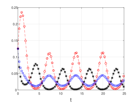
Figure 1: Probabilities $x_{1}(t)$ (black asterisk‬‏), $x_{4}(t)$ (blue square), and $x_{8}(t)$ (red circle) as a function of $t$ in Example 10.

Entrainment of the probabilities $x_{i}$ has consequences for other quantities of interest in statistical mechanics. For instance, an imporatnt quantity is the occupation density, i.e., the probability that site $s_{k}$ is occupied, often denoted by $\langle\tau_{k}\rangle$, cf. [35, 36]. Denoting the $k$-th component of the configuration $C_{i}\in\{0,1\}^{n}$ by $C_{i,k}$, a straightforward computation reveals that

$$\langle\tau_{k}(t)\rangle=\sum_{i=1}^{N}C_{i,k}x_{i}(t).$$

It is thus immediate that the occupation densities also converge to a unique periodic solution.

This phenomenon has already been observed empirically in Ref. [27] that studied a semi-infinite and finite TASEP coupled at the end to a reservoir with a periodic time-varying particle density. This models for example a traffic lane ending with a periodically-varying traffic light. The simulations in [27] suggest that this leads to the development of a sawteeth density profile along the chain, and that “The sawteeth profile is changing with time, but it regains its shape after each complete period…” [27, p. 011122-2] (see also [28, 29] for some related considerations).

Our results can also be interpreted in terms of the particles along the chain in TASEP. Since the expectation of the occupation densities $\langle\tau_{k}\rangle$ converges to a periodic solution, this means that in the long term the TASEP dynamics “fluctuates” around a periodic “mean” solution (see e.g. the simulation results depicted in Figure 5 in [30]). Moreover, in [28, 29] it was found for closely related models that the limiting periodic density profiles (whose existence is also guaranteed by our results) have an interesting structure that depends in a non-trivial way on the frequency of the transition rates.

III-B Entrainment in a stochastic SIS model

The stochastic susceptible-infected-susceptible (SIS) model plays an important role in mathematical epidemiology [37]. But, as noted in [38], it is usually studied under the assumption of fixed contact and recovery rates. Here, we apply our results to prove entrainment in an SIS model with periodic rates.

Consider a population of size $N$ divided into susceptible and infected individuals. Let $S(t)$ [$I(t)$] denote the size of the susceptible [infected] part of the population at time $t$, so that $S(t)+I(t)\equiv N$. We assume two mechanisms for infection. The first is by contact with an infected and depends on the contact rate $a(t)$. The second is by some external agent (modeling, say, insect bite) with rate $c(t)$. The recovery rate is $b(t)$. We assume that $a(t)$, $b(t)$, and $c(t)$ are continuous and take non-negative values for all time $t$.

If $I(t)=n$ (so $S(t)=N-n$) then the probability that one individual recovers in the time interval $[t,t+\mathop{}\!\mathrm{d}t]$ is $b(t)n\mathop{}\!\mathrm{d}t+o(\mathop{}\!\mathrm{d}t)$, and the probability for one new infection to occur in this time interval is $a(t)n\frac{N-n}{N}\mathop{}\!\mathrm{d}t+c(t)\frac{N-n}{N}\mathop{}\!\mathrm{d}t+o(\mathop{}\!\mathrm{d}t)$. For $n\in\{0,\dots,N\}$, let $P_{n}(t)$ denote the probability that $I(t)=n$. This yields the master equation:

$$\dot{P}_{n}=((n-1)a+c)\left(1-\frac{n-1}{N}\right)P_{n-1}-\left((na+c)(1-\frac{n}{N})+nb\right)P_{n}+(n+1)bP_{n+1},$$ (15)

for $n\in\{0,1,\dots,N\}$, where we define $P_{-1}=P_{N+1}:=0$, and for simplicity omit the dependence on $t$. This set of $N+1$ equations may be written in matrix form as

$$\dot{x}=Mx,$$

where $x:=\begin{bmatrix}P_{0}&P_{1}&\dots&P_{N}\end{bmatrix}^{\prime}\in[0,1]^{N+1}$, $M:=P-D$, with $D:=\operatorname{{\mathrm{d}iag}}(0,b,2b,\dots,Nb)$, and $P$ is the $(N+1)\times(N+1)$ matrix:

$$\begin{bmatrix}-cq_{0}&b&0&0&\dots&0&0&0\\ cq_{0}&-(a+c)q_{1}&2b&0&\dots&0&0&0\\ 0&(a+c)q_{1}&-(2a+c)q_{2}&3b&\dots&0&0&0\\ 0&0&(2a+c)q_{2}&-(3a+c)q_{3}&\dots&0&0&0\\ &&&&\vdots\\ 0&0&0&0&\dots&((N-2)a+c))q_{N-2}&-((N-1)a+c)q_{N-1}&bN\\ 0&0&0&0&\dots&0&((N-1)a+c)q_{N-1}&0\end{bmatrix},$$

where $q_{i}:=1-\frac{i}{N}$. Note that $M(t)$ is Metzler, as $a(t),b(t)$ and $c(t)$ are non-negative for all $t$. Thus, Theorems 5 and 8 yield the following result.

Corollary 11.

If $a(t)$, $b(t)$ and $c(t)$ are all $T$-periodic then any solution of (15) with $x(0)\in\Omega\subset\mathbb{R}^{N+1}$ converges to a $T$-periodic solution. Furthermore, if there exists a time $t^{*}\geq 0$ such that

$$b(t^{*})c(t^{*})>0$$ (16)

then there exists a unique $T$-periodic solution $\gamma$ in $\Omega$ and every solution converges to $\gamma$.

Example 12.

Consider the stochastic SIS model with $N=3$, $a(t)=1$, $b(t)=3+3\cos(t+0.5)$ and $c(t)=2-2\sin(t+0.75)$. These rates are non-negative and jointly $T$-periodic for $T=2\pi$ and clearly there exists $t^{*}\geq 0$ such that $b(t^{*})c(t^{*})>0$. Fig. 2 depicts $P_{i}(t)$, $i=0,1,2$, (note that $P_{3}(t)=1-P_{0}(t)-P_{1}(t)-P_{2}(t))$ as a function of time $t$ for the initial condition $P(0)=(1/4)1_{4}\in\Omega$. It may be seen that every $P_{i}(t)$ converges to a periodic solution with period $2\pi$. Taking other initial conditions $x(0)\in\Omega$ yields convergence to the same periodic solution.

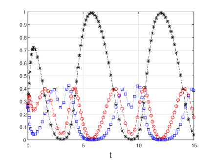
Figure 2: Probabilities $P_{0}(t)$ (black asterisk‬‏), $P_{1}(t)$ (red circle), and $P_{2}(t)$ (blue square) as a function of $t$ in Example 12.

Note that if the irreducibility condition (16) does not hold then the system may have several periodic solutions. To see this, consider for example the case $b(t)=c(t)\equiv 0$. Let $e^{i}\in\mathbb{R}^{N+1}$ denote the vector with entry $i$ equal to one and all other entries zero. Then both $x(t)\equiv e^{1}$ and $x(t)\equiv e^{N+1}$ are (periodic) solutions of the dynamics.

IV Discussion

In his 1929 paper on periodicity in disease prevalence, H. E. Soper [39] states: “Perhaps no events of human experience interest us so continuously, from generation to generation, as those which are, or seem to be, periodic”. Soper also raised the question of whether the observed periodicity in epidemic outbreaks is the result of a “seasonal change in perturbing influences, such as might be brought about by school break-up and reassembling, or other annual recurrences?” In modern terms, this amounts to asking whether the solutions of the system describing the dynamics of the epidemics entrain to periodic variations in the transmission parameters.

Here, we studied entrainment for dynamical systems described by a master equation. We considered a rather general formulation where the transition rates may depend on both time and state. Also, we did not assume any symmetry conditions (e.g. detailed balance conditions [3, Ch. V]) on the rates. We note that this formulation implies similar results for non-linear systems as well. Indeed, consider the time-varying non-linear system:

$$\dot{x}=f(t,x),$$ (17)

and assume that $f(t,0)=0$ for all $t$. Let $J(t,x):=\frac{\partial f}{\partial x}(t,x)$ denote the Jacobian of the vector field. Then

$$\dot{x} =\int_{0}^{1}\frac{d}{ds}f(t,sx)\mathop{}\!\mathrm{d}s$$

$$=A(t,x)x,$$

where $A(t,x):=\int_{0}^{1}J(t,sx)\mathop{}\!\mathrm{d}s$. If $A(t,x)$ has the form (12) then the results above can be applied to (17).

We proved that entrainment indeed holds under quite mild technical conditions. This follows from the fact that the master equation is a cooperative dynamical system admitting a first integral. Due to the prevalence of the master equation as a model for natural and artificial phenomena, we believe that this result will find many applications. To demonstrate this, we described two applications of our results: a proof of entrainment in TASEP and in a stochastic SIS model.

The rigorous proof that the solutions of the master equation entrain is of course a necessary first step in studying the structure of the periodic trajectory (or trajectories), and its dependence on various parameters. Indeed, in many applications it is of interest to obtain more information on the periodic trajectory e.g. its amplitude. Of course, one cannot expect in general to obtain a closed-form description of the limit cycle. However, for contractive dynamical systems there do exist efficient methods for obtaining a closed-form approximation of the limit cycle accompanied by explicit error bounds [16]. Developing a similar approach for the attractive limit cycle of the master equation may be an interesting topic for further research. In the specific case of TASEP with fixed rates, there exists a powerful representation of the steady-state in terms of a product of matrices [35, 7]. It may be of interest to try and represent the periodic steady-state using a similar product, but with matrices with periodic entries. This could be used in particular to study the effects of periodic perturbations to the boundary-induced phase transitions that have been observed for TASEP in [40].

Competing Interests

The authors have no competing interests.

Author Contributions

MM, LG, and TK performed the research and wrote the paper.

V Appendix: Proofs of Theorems 5 and 8

The proofs of Theorems 5 and 8 are based on known tools from the theory of monotone dynamical systems admitting a first integral with a positive gradient (see, e.g. [41, 42, 43]). We present in this appendix a self-contained proof taking full advantage of the technical simplifications that our specific setting permits. This, in particular, allows us to prove that the results hold on the closed state-space and also that irreducibility at a single time point is enough to guarantee convergence to a unique periodic solution. Without loss of generality we always assume that the initial time is $t_{0}=0$. It is convenient to work with the $\ell_{1}$ vector norm $|{x}|_{1}=\sum_{i}|{x}_{i}|$.

We begin by introducing some notation. First recall the notation

$$\mathbb{R}^{N}_{+}:=\{x\in\mathbb{R}^{N}\,|\,x_{j}\geq 0\mbox{ for all }1\leq j\leq N\}$$

for the closed positive cone. Define a set of vector fields by:

$$\mathcal{F} := \{f:[0,\infty)\times\mathbb{R}^{N}_{+}\to\mathbb{R}^{N}\,|\,\mbox{properties (i)--(v) below are satisfied}\},$$

where

1. $f$ is continuous;

2. for all $j\in\{1,\ldots,N\}$, $\frac{\partial f}{\partial x_{j}}(t,x)$ exists for $(t,x)\in[0,\infty)\times\operatorname{{\mathrm{i}nt}}(\mathbb{R}^{N}_{+})$ and has a continuous extension onto $[0,\infty)\times\mathbb{R}^{N}_{+}$. Thus, $J(t,x)$ from (13) is defined on $[0,\infty)\times\mathbb{R}^{N}_{+}$ to be the continuous extension of $\frac{\partial f}{\partial x_{j}}(t,x)$;

3. $J(t,x)$ is Metzler for all $(t,x)\in[0,\infty)\times\mathbb{R}^{N}_{+}$;

4. $\sum_{i=1}^{N}f_{i}(t,x)=0$ for all $(t,x)\in[0,\infty)\times\mathbb{R}^{N}_{+}$;

5. $f(t,0)=0$ for all $t\in[0,\infty)$.

For $T>0$, let $\mathcal{F}_{T}:=\{f\in\mathcal{F}\,|\,f(t+T,x)=f(t,x)\mbox{ for all }(t,x)\in[0,\infty)\times\mathbb{R}^{N}_{+}\}$, that is, the set of vector fields in $\mathcal{F}$ that are also $T$-periodic.

It is straightforward to check that $f(t,x)=A(t,x)x$ with $A$ defined by (12) belongs to $\mathcal{F}_{T}$ if Assumption 4 and the assumptions of Theorem 5 hold. Therefore, Theorem 5 follows from the following result.

Theorem 13.

If $f\in\mathcal{F}_{T}$ then for all $x_{0}\in\Omega$ the solution $x(t;x_{0})$ of the initial value problem

$$\dot{x}=f(t,x),\quad x(0)=x_{0},$$

is asymptotically $T$-periodic, i.e., there exists a solution $\gamma:\mathbb{R}\to\Omega$ of $\dot{\gamma}=f(t,\gamma)$, with $\gamma(t+T)=\gamma(t)$ for all $t\in\mathbb{R}$, and

$$\lim_{t\to\infty}|x(t;x_{0})-\gamma(t)|_{{1}}=0.$$

Let

$$\mathcal{F}_{\text{irr}}^{\Omega}:=\{f\in\mathcal{F}\,|\,\text{there exists }t^{*}\geq 0\text{ such that }J(t^{*},x)\text{ is irreducible for all }x\in\Omega\}.$$

The next result is a generalization of Theorem 8.

Theorem 14.

If $f\in(\mathcal{F}_{T}\cap\mathcal{F}_{\text{irr}}^{\Omega})$ then the differential equation $\dot{x}=f(t,x)$ admits a unique $T$-periodic solution $\gamma:\mathbb{R}\to\Omega$. Moreover, there exists $\alpha>0$ such that for any initial condition $x_{0}\in\Omega$ the corresponding solution $x(t;x_{0})$ satisfies

$$|x(t;x_{0})-\gamma(t)|_{1}<2e^{-\alpha t}|x_{0}-\gamma(0)|_{1},$$

i.e. the solution converges to $\gamma$ with exponential rate $\alpha$.

Complete proofs of Theorem 13 and Theorem 14 are provided in the following seven subsections. We begin by showing in Lemma 16 that solutions of $\dot{x}=f(t,x)$, $f\in\mathcal{F}$, that start in the closed state space $\mathbb{R}_{+}^{N}$ are unique and remain in $\mathbb{R}_{+}^{N}$ for all positive times. In the second subsection, we prove that for the subset of linear vector fields $f$ in $\mathcal{F}$ the flow is cooperative, and non-expansive or even contractive in the case of irreducibility. The latter property is then generalized to the nonlinear setting (Theorem 20), which is enough to prove Theorem 14 in Subsection V-D. The cooperative behavior for nonlinear vector fields is stated in Theorem 21. In Subsection V-F, we argue that the non-expansiveness of the flow together with the existence of a fixed point in the $\omega$-limit set of the period map implies the asymptotic periodicity of the solution. The proof that such a fixed point exists is deferred to the final subsection. It uses the cooperative behavior of the flow as well as the fact that the first integral $H$ has a positive gradient, i.e. $\nabla H\in$ int$(\mathbb{R}_{+}^{N})$.

V-A Positive invariance of $\mathbb{R}^{N}_{+}$

Our first goal is to establish in Lemma 16 below that for any $x_{0}\in\mathbb{R}^{N}_{+}$ a unique solution $x(t;x_{0})$ exists for all $t\in[0,\infty)$ and remains in the closed cone $\mathbb{R}^{N}_{+}$. Denote

$$\mathcal{B}:=\left\{B\in\mathbb{R}^{N\times N}\,\left|\,B\mbox{ is Metzler and }\sum_{i=1}^{N}B_{ij}=0\mbox{ for all }j\in\{1,\ldots,N\}\right.\right\}.$$

Proposition 15.

Assume that $f\in\mathcal{F}$. Then there exists a continuous map $B:[0,\infty)\times\mathbb{R}^{N}_{+}\times\mathbb{R}^{N}_{+}\to\mathcal{B}$ such that

$$f(t,x)-f(t,y)=B(t,x,y)(x-y)\text{ for all }t\geq 0\text{ and all }x,y\in\mathbb{R}^{N}_{+}.$$ (18)

Moreover, for any index $j$ the following property holds. If $x\in\mathbb{R}^{N}_{+}$ with $x_{j}=0$ then $f_{j}(t,x)\geq 0$ for all $t\geq 0$.

Proof. Eq. (18) follows from the fundamental theorem of calculus with

$$B(t,x,y)=\int_{0}^{1}J(t,y+s(x-y))\mathop{}\!\mathrm{d}s\text{ for all }t\geq 0\text{ and }x,y\in\operatorname{{\mathrm{i}nt}}(\mathbb{R}^{N}_{+}).$$

By assumptions (iii) and (iv) on $f$ we conclude that $B(t,x,y)\in\mathcal{B}$. Moreover, assumption (ii) implies that this formula actually defines $B$ as a continuous map on $[0,\infty)\times\mathbb{R}_{+}^{N}\times\mathbb{R}_{+}^{N}$ into $\mathcal{B}$. Eq. (18) also holds on the closed cone $\mathbb{R}_{+}^{N}$ due to assumption (i). The second claim follows from $f(t,x)=B(t,x,0)x$ and the fact that $B(t,x,0)$ is Metzler. ∎

Lemma 16.

Assume that $f\in\mathcal{F}$. Then for every $x_{0}\in\mathbb{R}^{N}_{+}$ the initial value problem $\dot{x}=f(t,x)$, $x(0)=x_{0}$, admits a unique solution $x(\,\cdot\,;x_{0}):[0,\infty)\to\mathbb{R}^{N}_{+}$. Moreover,

$$H(x)=\sum_{j=1}^{N}x_{j}$$

is a first integral of the dynamics, i.e., $\frac{d}{dt}H(x(t;x_{0}))\equiv 0$.

Proof. By assumption (i) on $f$ and by Proposition 15, the vector field $f$ satisfies the hypotheses of the Picard-Lindelöf Theorem, however with a domain of definition $\mathbb{R}^{n}_{+}$ which is not open. Introduce the auxiliary extension

$$\tilde{f}(t,x):=f(t,|x_{1}|,\ldots,|x_{N}|).$$

Note that $\tilde{f}:[0,\infty)\times\mathbb{R}^{N}\to\mathbb{R}^{N}$ is well-defined. The Picard-Lindelöf Theorem yields existence and uniqueness of a maximal solution $\tilde{x}(\,\cdot\,;x_{0}):J_{x_{0}}\to\mathbb{R}^{N}$ of the initial value problem $\dot{x}=\tilde{f}(t,x)$, $x(0)=x_{0}$, with $J_{x_{0}}=[0,b_{x_{0}})$ for some $b_{x_{0}}>0$ that might be infinite. Note that $H$ is a first integral by property (iv) of $f$, that carries over to $\tilde{f}$.

On $\mathbb{R}^{N}_{+}$, the solutions $x(\,\cdot\,;x_{0})$ and $\tilde{x}(\,\cdot\,;x_{0})$ coincide. We now show that for $x_{0}\in\mathbb{R}^{N}_{+}$ the solution $\tilde{x}(t;x_{0})\in\mathbb{R}^{N}_{+}$ for all $t\in J_{x_{0}}$. If $x_{0}=0$ then $\tilde{x}(t;x_{0})\equiv 0$ by assumption (v) on $f$, so $\tilde{x}(t;x_{0})\in\mathbb{R}^{N}_{+}$. If $x_{0}\in\mathbb{R}^{N}_{+}\setminus\{0\}$, we argue by contradiction. Assume that there exists $\tau>0$ such that $\tilde{x}(\tau;x_{0})\in(\mathbb{R}^{N}\setminus\mathbb{R}^{N}_{+})$. For $\varepsilon\in\mathbb{R}$, let

$$\tilde{f}_{\varepsilon}:[0,\infty)\times\mathbb{R}^{N}\to\mathbb{R}^{N},\;\;\tilde{f}_{\varepsilon}(t,x):=\tilde{f}(t,x)+\varepsilon\left(\begin{array}[]{ccc}1&\cdots&1\\ \vdots&\vdots&\vdots\\ 1&\cdots&1\end{array}\right)x-\varepsilon Nx,$$

and denote by $\tilde{x}(\cdot;x_{0},\varepsilon)$ the unique maximal solution of $\dot{x}=\tilde{f}_{\varepsilon}(t,x)$, $x(0)=x_{0}$. Note that by the definition of $\tilde{f}_{\varepsilon}$ the function $H$ is also a first integral for this dynamical system.

Now by the continuous dependence of solutions on parameters there exists $\varepsilon_{0}>0$ such that $\tilde{x}(\tau;x_{0},\varepsilon_{0})\in(\mathbb{R}^{N}\setminus\mathbb{R}^{N}_{+})$. This implies that there exists a time $s\in[0,\tau)$ such that $x(s;x_{0},\varepsilon_{0})$ leaves $\mathbb{R}^{N}_{+}$, i.e. there exists $k\in\{1,\ldots,N\}$ with $\tilde{x}_{k}(s;x_{0},\varepsilon_{0})=0$ and $\dot{\tilde{x}}_{k}(s;x_{0},\varepsilon_{0})\leq 0$. However, this is a contradiction, since

$$\dot{\tilde{x}}_{k}(s;x_{0},\varepsilon_{0}) =(\tilde{f}_{\varepsilon}(s,\tilde{x}(s;x_{0},\varepsilon_{0})))_{k}$$

$$\geq\varepsilon_{0}\sum_{j\neq k}\tilde{x}_{j}(s;x_{0},\varepsilon_{0})$$

$$=\varepsilon_{0}H(x_{0})$$

$$>0,$$

where the first inequality follows from Proposition 15 and the definition of $\tilde{f}_{\varepsilon}$, and the last equality follows from the fact that $H$ is also a first integral for $\dot{x}=\tilde{f}_{\varepsilon}(t,x)$.

We have established that $\tilde{x}$ remains in the compact set $\{z\in\mathbb{R}_{+}^{N}\,|\,H(z)=H(x_{0})\}$ and it follows that the solution $\tilde{x}(t;x_{0})$ exists for all $t\geq 0$. Since the solutions $x(\,\cdot\,;x_{0})$ and $\tilde{x}(\,\cdot\,;x_{0})$ coincide on $\mathbb{R}_{+}^{N}$, this completes the proof. ∎

V-B Linear time-varying systems

The properties that are essential in the proofs of our main results are cooperativeness, non-expansiveness, and contractivity of the flow. As it turns out, it is convenient to first prove these properties for linear time-varying systems. Let

$$\mathcal{A}:=\{A:[0,\infty)\to\mathcal{B}\,|\,A\mbox{ is continuous}\}.$$

Lemma 17.

Assume that $A\in\mathcal{A}$. Then the initial value problem $\dot{x}=A(t)x$, $x(0)=x_{0}\in\mathbb{R}^{N}_{+}$, has a unique solution $x(\,\cdot\,;x_{0}):[0,\infty)\to\mathbb{R}^{N}$ that satisfies the following properties:

1. $x(t;x_{0})\in\mathbb{R}^{N}_{+}$ and $H(x(t;x_{0}))=H(x_{0})$ for all $t\geq 0$.

2. If $x_{j}(t^{*};x_{0})>0$ for some $j\in\{1,\ldots,N\}$ and $t^{*}\geq 0$ then $x_{j}(t;x_{0})>0$ for all $t\geq t^{*}$.

3. If $x_{0}\not=0$ and $A(t^{*})$ is irreducible for some $t^{*}\geq 0$ then $x(t;x_{0})\in\operatorname{{\mathrm{i}nt}}(\mathbb{R}^{N}_{+})$ for all $t>t^{*}$.

Proof. Existence and uniqueness of the solution are immediate from the linearity and continuity of $A$.

The proof of a) follows from Lemma 16 and the fact that $f(t,x):=A(t)x$ belongs to $\mathcal{F}$ for each $A\in\mathcal{A}$.

To prove b), assume that $x_{j}(t^{*};x_{0})>0$. Let $y(t):=x_{j}(t;x_{0})$. Then $y$ solves the scalar initial value problem

$$\dot{y}=g(t,y),\quad y(t^{*})=x_{j}(t^{*};x_{0})>0$$

where

$$g(t,y):=a_{jj}(t)y+b(t),\quad b(t):=\sum_{k\neq j}a_{jk}(t)x_{k}(t;x_{0})\geq 0.$$

Thus, letting $q(t):=\int_{t^{*}}^{t}a_{jj}(u)\mathop{}\!\mathrm{d}u$ yields

$$y(t) =e^{q(t)}\left(y(t^{*})+\int_{t^{*}}^{t}e^{-q(s)}b(s)\mathop{}\!\mathrm{d}s\right)$$

$$\geq e^{q(t)}y(t^{*})$$

$$>0$$

for all $t\geq t^{*}$.

To prove property c) first note that irreducibility of $A(t^{*})$ implies that there exists $\delta>0$ such that

$$A(t)\text{ is irreducible for all }t\in[t^{*},t^{*}+\delta).$$ (19)

This follows from the fact that irreducibility is equivalent to the associated adjacency graph being strongly connected, i.e. certain edges have positive weights, and the continuity of $A(t)$.

Pick $x_{0}\in\mathbb{R}^{n}_{+}\setminus\{0\}$. We consider two cases.

Case 1: $x(t^{*};x_{0})\in\operatorname{{\mathrm{i}nt}}(\mathbb{R}^{N}_{+})$. Then the claim follows from property b).

Case 2: $x(t^{*};x_{0})\in\partial\mathbb{R}^{N}_{+}$. Fix $t>t^{*}$. As $H(x(t^{*};x_{0}))=H(x_{0})>0$, there exists $k\in\{1,\ldots,N-1\}$ such that exactly $k$ entries of $x(t^{*};x_{0})$ are positive and the other entries are zero. Note that by property b), these $k$ entries remain positive for all $t\geq t^{*}$. Assume w.l.o.g. that the first $k$ entries of $x(t^{*};x_{0})$ are positive. Then in block form

$$\dot{x}(t^{*};x_{0})=\left(\begin{array}[]{c|c}U&V\\ \hline\cr Y&Z\end{array}\right)\left(\begin{array}[]{c}x_{1}(t^{*};x_{0})\\ \vdots\\ x_{k}(t^{*};x_{0})\\ \hline\cr 0\end{array}\right),$$

with $U\in\mathbb{R}^{k\times k}$ and $Z\in\mathbb{R}^{(N-k)\times(N-k)}$. Since $A(t^{*})$ is Metzler and irreducible, every entry of $Y$ is non-negative and at least one entry is positive, so there exists $j>k$ such that $\dot{x}_{j}(t^{*};x_{0})>0$. Therefore, at least $k+1$ entries of $x(t;x_{0})$ are positive for $t>t^{*}$. Now an inductive argument and using (19) completes the proof. ∎

Let

$$\mathcal{S}:=\left\{Q\in\mathbb{R}^{N\times N}\,\left|\,q_{jk}\geq 0\mbox{ for all }j,k=1,\ldots,N\text{ and }\sum_{j=1}^{N}q_{jk}=1\text{ for all }k=1,\ldots,N\right.\right\}$$

denote the set of of $N\times N$ stochastic matrices, and let

$$\mathcal{S}^{+}:=\{Q\in\mathcal{S}\,|\,q_{jk}>0\mbox{ for all }j,k=1,\ldots,N\}$$

denote the subset of stochastic matrices with positive entries. For $A\in\mathcal{A}$ let $\Phi_{A}:[0,\infty)\to\mathbb{R}^{N\times N}$ be the fundamental matrix of $\dot{x}=Ax$, that is, the solution of

$$\dot{\Phi}(t)=A(t)\Phi(t),\quad\Phi(0)=I_{N}.$$

Since the columns of $\Phi_{A}(t)$ are $x(t;e^{j})$, where $e^{j}\in\mathbb{R}^{N}_{+}$ denotes the $j$-th canonical unit vector, the next result follows from Properties a) and c) in Lemma 17.

Corollary 18.

Assume that $A\in\mathcal{A}$. Then

1. $\Phi_{A}(t)\in\mathcal{S}$ for all $t\geq 0$.

2. If $A(t^{*})$ is irreducible for some $t^{*}\geq 0$ then $\Phi_{A}(t)\in\mathcal{S}^{+}$ for all $t>t^{*}$.

We now use this to prove non-expansiveness with respect to the $\ell_{1}$-norm and contractivity in the case of irreducibility. The first step is to note that stochastic matrices have useful properties with respect to this norm.

Proposition 19.

If $Q\in\mathcal{S}$ and $x\in\mathbb{R}^{N}$ then $|Qx|_{1}\leq|x|_{1}$. If $Q\in\mathcal{S}^{+}$ and $x\in(\mathbb{R}^{n}\setminus\{0\})$ with $H(x)=0$ then $|Qx|_{1}<|x|_{1}$.

Proof. The first statement follows from

$$|Qx|_{1} =\sum_{j=1}^{N}\left|\sum_{k=1}^{N}Q_{jk}x_{k}\right|$$

$$\leq\sum_{j=1}^{N}\sum_{k=1}^{N}Q_{jk}|x_{k}|$$

$$=\sum_{k=1}^{N}|x_{k}|$$

$$=|x|_{1}.$$ (20)

To prove the second statement, pick $x\neq 0$ such that $H(x)=0$. Then there exist $k_{1},k_{2}\in\{1,\ldots,N\}$ such that $x_{k_{1}}<0<x_{k_{2}}$. Thus, if $Q\in\mathcal{S}^{+}$ then for any $j\in\{1,\ldots,N\}$,

$$\left|\sum_{k=1}^{N}Q_{jk}x_{k}\right|<\sum_{k=1}^{N}Q_{jk}|x_{k}|$$

because the sum on the left contains both positive and negative terms. Now arguing as in (V-B) completes the proof. ∎

V-C Non-expansiveness and contractivity

Using the results for time-varying linear systems we now turn to proving non-expansiveness and contractivity for the nonlinear dynamical system.

Theorem 20.

Suppose that $f\in\mathcal{F}$. Then

1. For any $x_{0},y_{0}\in\mathbb{R}^{N}_{+}$ the function

   $$t\mapsto|x(t;x_{0})-x(t;y_{0})|_{1}\text{ is non-increasing on }[0,\infty).$$ (21)

2. If there exists $t^{*}\geq 0$ such that $J(t^{*},x)$ is irreducible for all $x\in\Omega$ then for any $\hat{t}>t^{*}$ there exists $M_{\hat{t}}<1$ such that

   $$|x(\hat{t};x_{0})-x(\hat{t};y_{0})|_{1}\leq M_{\hat{t}}|x_{0}-y_{0}|_{1}\quad\text{for all }x_{0},y_{0}\in\Omega.$$ (22)

Proof. Fix $t_{1}\geq 0$ and $x_{0},y_{0}\in\Omega$. Let $z(t):=x(t+t_{1};x_{0})-x(t+t_{1};y_{0})$. By Proposition 15, $\dot{z}(t)=C(t)z(t)$, with $z(0)=z_{0}:=x(t_{1};x_{0})-x(t_{1};y_{0})$, and $C\in\mathcal{A}$ given by

$$C(t):=B(t+t_{1},x(t+t_{1};x_{0}),x(t+t_{1};y_{0}))$$

for all $t\geq 0$. Hence, $z(t)=\Phi_{C}(t)z_{0}$ for all $t\geq 0$.

To prove (21), pick $t_{2}\geq t_{1}$. By Corollary 18a), $\Phi_{C}(t_{2}-t_{1})\in\mathcal{S}$ and Proposition 19 yields

$$|x(t_{2};x_{0})-x(t_{2};y_{0})|_{1} =|z(t_{2}-t_{1})|_{1}$$

$$=|\Phi_{C}(t_{2}-t_{1})z_{0}|_{1}$$

$$\leq|z_{0}|_{1}$$

$$=|x(t_{1};x_{0})-x(t_{1};y_{0})|_{1},$$

and this proves (21).

To prove (22), let

$$\mathcal{P}:=\{x\in\mathbb{R}^{N}\,|\,H(x)=0\text{ and }|x|_{1}=1\}.$$

Note that if $y,z\in\Omega$ with $y\not=z$ then $\frac{y-z}{|y-z|_{1}}\in\mathcal{P}$.

Pick $\hat{t}>t^{*}$ and $x_{0},y_{0}\in\Omega$. Eq. (22) clearly holds if $x_{0}=y_{0}$, so we may assume that $x_{0}\not=y_{0}$. Then

$$|x(\hat{t};x_{0})-x(\hat{t};y_{0})|_{1} =|\Phi_{C}(\hat{t})(x_{0}-y_{0})|_{1}$$

$$=m\left(x_{0},y_{0},\frac{x_{0}-y_{0}}{|x_{0}-y_{0}|_{1}}\right)|x_{0}-y_{0}|_{1},$$

where $m:\Omega\times\Omega\times\mathcal{P}\to\mathbb{R}$ is defined by $m(x_{0},y_{0},v):=|\Phi_{C}(\hat{t})v|_{1}$. Let

$$M_{\hat{t}}:=\max\{m(x,y,v)\;|\;x\in\Omega,y\in\Omega,v\in\mathcal{P}\}.$$

This is well-defined, as the matrix $C(t)=C_{x_{0},y_{0}}(t)=B(t,x(t;x_{0}),x(t;y_{0}))$ depends continuously on $x_{0},y_{0}\in\Omega$ for all $t\geq 0$ (see Proposition 15) and thus $\Phi_{C_{x_{0},y_{0}}}(\hat{t})$ is also continuous in $x_{0},y_{0}$. We conclude that

$$|x(\hat{t};x_{0})-x(\hat{t};y_{0})|_{1} \leq M_{\hat{t}}|x_{0}-y_{0}|_{1}.$$

Thus, to complete the proof we only need to show that $M_{\hat{t}}<1$. To prove this, denote $x^{*}:=x(t^{*};x_{0})$, $y^{*}:=x(t^{*};y_{0})$. Then

$$C_{x_{0},y_{0}}(t^{*})=B(t^{*},x^{*},y^{*})=\int_{0}^{1}J(t^{*},y^{*}+s(x^{*}-y^{*}))\mathop{}\!\mathrm{d}s.$$

Since $J$ is Metzler (i.e. all its off diagonal elements are non-negative) and, by assumption, $J(t^{*},z)$ is irreducible for all $z\in\Omega$, we conclude that $C_{x_{0},y_{0}}(t^{*})$ is also irreducible. Corollary 18 implies that $\Phi_{C_{x_{0},y_{0}}}(\hat{t})\in\mathcal{S}^{+}$. Picking a maximizer $(x_{0},y_{0},v_{0})\in\Omega\times\Omega\times\mathcal{P}$ of $m$, i.e. $M_{\hat{t}}=m(x_{0},y_{0},v_{0})$, it follows from Proposition 19 that $M_{\hat{t}}<|v_{0}|_{1}=1$. ∎

V-D Proof of Theorem 14

We can now prove Theorem 14. We note that the proof proceeds without the explicit use of the cooperative behavior of dynamical systems (though we will use this property for the proof of Theorem 13; see Subsections V-E, V-F below).

Note that for $f\in\mathcal{F}_{T}$ a solution $\dot{\gamma}=f(t,\gamma)$, $\gamma:[0,\infty)\to\Omega$, is $T$-periodic if and only if $x(T;\gamma(0))=\gamma(0)$. Thus, consider the period map $P_{T}:\mathbb{R}^{N}_{+}\to\mathbb{R}^{N}_{+}$ defined by

$$P_{T}(a):=x(T;a).$$ (23)

In other words, $P_{T}(a)$ is the value of $x(T)$ for the initial condition $x(0)=a$. Observe that $P_{T}(\Omega)\subseteq\Omega$ (as $H$ is a first integral of $\dot{x}=f(t,x)$). Moreover, for $f\in(\mathcal{F}_{T}\cap\mathcal{F}^{\Omega}_{\text{irr}})$ there exists $t^{*}\in[0,T)$ such that $J(t^{*},x)$ is irreducible for all $x\in\Omega$. Then $T>t^{*}$, so Theorem 20b) implies that $P_{T}$ is Lipschitz on the closed set $\Omega$ with Lipschitz constant $M_{T}<1$. The Banach fixed point theorem implies that $P_{T}$ has a unique fixed point in $\Omega$, that is, there exists a unique $T$-periodic function $\gamma:\mathbb{R}\to\Omega$ that solves $\dot{\gamma}=f(t,\gamma)$. Fix $\alpha>0$ such that

$$\max\{1/2,M_{T}\}\leq e^{-\alpha T}.$$ (24)

Pick $x_{0}\in\Omega$ and $t\geq 0$, and let $k\in\mathbb{N}_{0}$ be such that $kT\leq t\leq(k+1)T$. Then Theorem 20 yields

$$|x(t;x_{0})-\gamma(t)|_{1} \leq|x(kT;x_{0})-\gamma(kT)|_{1}$$

$$\leq(M_{T})^{k}|x_{0}-\gamma(0)|_{1}$$

$$\leq e^{-\alpha Tk}|x_{0}-\gamma(0)|_{1}$$

$$=e^{-\alpha T(k+1)}e^{\alpha T}|x_{0}-\gamma(0)|_{1}$$

$$\leq e^{\alpha T}e^{-\alpha t}|x_{0}-\gamma(0)|_{1}$$

$$\leq 2e^{-\alpha t}|x_{0}-\gamma(0)|_{1}.$$

where the last inequality follows from (24). Thus, every solution $x(t;x_{0})$ converges to the unique periodic solution $\gamma(t)$ at an exponential rate. ∎

V-E Cooperative behavior

For the proof of Theorem 13 we use some elegant topological ideas from [43, 42], which are based on the cooperative behavior of the dynamical system generated by a vector field $f\in\mathcal{F}$. In order to formulate this concept we introduce some more notation.

Let $p,q\in\mathbb{R}^{N}$, and let $A$ be a bounded non-empty subset of $\mathbb{R}^{N}$. Then we write

1. $p\leq q$ $:\Leftrightarrow$ $p_{j}\leq q_{j}$ for all $j\in\{1,\ldots,N\}$,

2. $[p,q]:=\{x\in\mathbb{R}^{N}\,|\,p\leq x\leq q\}$,

3. $\inf A:=c\in\mathbb{R}^{N}$ with $c_{j}:=\inf\{a_{j}\,|\,a\in A\}$,
   $\sup A:=d\in\mathbb{R}^{N}$ with $d_{j}:=\sup\{a_{j}\,|\,a\in A\}$,

4. $p\leq A$ $\Leftrightarrow$ $p\leq a$ for all $a\in A$
   $q\geq A$ $\Leftrightarrow$ $q\geq a$ for all $a\in A$,

It is straightforward to verify that $\inf A\leq A\leq\sup A$ and that for all $x,y\in\mathbb{R}^{N}$ with $x\leq A$, $y\geq A$ we have $x\leq\inf A$ and $y\geq\sup A$.

The following theorem summarizes the monotone behavior with respect to the order $\leq$.

Theorem 21.

Let $f\in\mathcal{F}$ and $x_{0},y_{0}\in\mathbb{R}^{N}_{+}$ with $x_{0}\leq y_{0}$. Then $x(t;x_{0})\leq x(t;y_{0})$ for all $t\geq 0$. If, in addition, $(x_{0})_{j}<(y_{0})_{j}$ for some $j\in\{1,\ldots,N\}$, then $x_{j}(t;x_{0})<x_{j}(t;y_{0})$ for all $t\geq 0$.

Proof. We use again that $z(t):=x(t;y_{0})-x(t;x_{0})$ solves $\dot{z}=C(t)z$, $z(0)=z_{0}:=y_{0}-x_{0}\in\mathbb{R}^{N}_{+}$ with $C(t):=B(t,x(t;y_{0}),x(t;x_{0}))\in\mathcal{B}$ and $C\in\mathcal{A}$. The claim then follows from statements a) and b) of Lemma 17. ∎

V-F $\omega$-Limit sets of $P_{T}$ and proof of Theorem 13

The concept of $\omega$-limit sets for the discrete time dynamical system induced by the period map $P_{T}:\Omega\to\Omega$ from (23) is pivotal for the proof of Theorem 13. For $a\in\Omega$ this set is

$$\omega_{T}(a):=\{x\in\Omega\,|\,\mbox{there is a sequence }n_{k}\to\infty\mbox{ with }\lim_{k\to\infty}P_{T}^{n_{k}}(a)=x\}.$$

We first state a few standard facts about this set.

Proposition 22.

Let $f\in\mathcal{F}$. Pick $T>0$. Then for all $a\in\Omega$ we have

1. $\omega_{T}(a)$ is a closed, nonempty subset of $\Omega$;

2. $P_{T}(\omega_{T}(a))=\omega_{T}(a)$;

3. $\omega_{T}(b)\subseteq\omega_{T}(a)$ for all $b\in\omega_{T}(a)$.

Proof. Statements a) and b) follow from [44, Eq. (4.7.2) and Lemma 4.7.4] because $P^{k}_{T}(a)$ evolves in the compact set $\Omega$.

To prove c), pick $b\in\omega_{T}(a)$. Property b) implies that $P^{n_{k}}_{T}(b)\in\omega_{T}(a)$ for all $n_{k}\in\mathbb{N}$, and since $\omega_{T}(a)$ is closed $\lim_{k\to\infty}P_{T}^{n_{k}}(b)\in\omega_{T}(a)$. ∎

The following lemma, that is proved in the subsequent subsection, provides all that is needed to prove Theorem 13.

Lemma 23.

Let $f\in\mathcal{F}_{T}$. Then for every $x\in\Omega$ its limit set $\omega_{T}(x)$ contains a fixed point of $P_{T}$.

Proof of Theorem 13.  Pick $x_{0}\in\Omega$ and denote by $z\in\omega_{T}(x_{0})$ the fixed point of $P_{T}$ that exists according to Lemma 23. Since $z$ is a fixed point and since $f\in\mathcal{F}_{T}$ is $T$-periodic, the solution $\gamma(t):=x(t;z)$ is also $T$-periodic. As $z\in\omega_{T}(x_{0})$ there exists a subsequence $P_{T}^{n_{k}}(x_{0})\to z$ as $k\to\infty$. For any $j\in\mathbb{N}$ and $t\geq n_{j}T$ we have by Theorem 20a),

$$|x(t;x_{0})-\gamma(t)|_{1}\leq|x(Tn_{j};x_{0})-\gamma(Tn_{j})|_{1}=|P_{T}^{n_{j}}(x_{0})-z|_{1}.$$

As $t\to\infty$, we can take $j\to\infty$ and this yields

$$\lim_{t\to\infty}|x(t;x_{0})-\gamma(t)|_{1}=0,$$

proving Theorem 13. ∎

Note that the proof of Theorem 13 shows that for any $x_{0}\in\Omega$ the $\omega$-limit set $\omega_{T}(x_{0})$ cannot contain more than one fixed point of $P_{T}$. Thus, the statement in Lemma 23 can actually be strengthened to $\omega_{T}(x_{0})$ contains exactly one fixed point of $P_{T}$.

The next subsection contains the proof of the crucial Lemma 23. We have adapted the ideas presented by J. Ji-Fa in [43] to our setting which led to somewhat simplified arguments. In particular, we can replace [42, Proposition 1] that is used in the proof of Lemma 3.2 of [43] by a standard application of Brouwer’s fixed point theorem. Indeed, the claim of Lemma 23 is the existence of a fixed point of the map $P_{T}$ in $\omega_{T}(x)$. We show that $\omega_{T}(x)$ contains an element $y$ so that $\omega_{T}(y)$ is a singleton, say, $\omega_{T}(y)=\{z\}$. Then $z\in\omega_{T}(x)$ by Proposition 22c) and $z$ is a fixed point by Proposition 22b).

V-G Proof of Lemma 23

We use the following notation. For $y\in\Omega$, let

$$p(y) :=\inf\omega_{T}(y),$$

$$q(y) :=\sup\omega_{T}(y).$$

Note that since $\omega_{T}(y)\subseteq\Omega\subset\mathbb{R}^{N}_{+}$, $p(y)$ and $q(y)$ exist in $\mathbb{R}^{N}_{+}$. Moreover, $p(y)\leq q(y)$ and $\omega_{T}(y)$ is a singleton if and only if $p(y)=q(y)$. The existence of the desired element $y$ in $\omega_{T}(x)$ is established by contradiction. Suppose that no such $y$ exists. Denote by $y_{0}$ an element in $\omega_{T}(x)$ that minimizes the number of coordinates $j$ for which $(p(y))_{j}$ and $(q(y))_{j}$ differ. We then show that there exists $z_{0}\in\omega_{T}(x)$ for which $p(z_{0})$ and $q(z_{0})$ differ in a smaller number of coordinates than $p(y_{0})$ and $q(y_{0})$. Part c) of Lemma 24 below states a fact that is essential for the construction of $z_{0}$. What is also crucial for the proof is the observation that $p(y)$ and $q(y)$ are fixed points of $P_{T}$ which is formulated in Lemma 24a). Its short proof demonstrates why monotone dynamical systems admitting a first integral with a positive gradient are special.

For $y\in\Omega$, let

$$J_{y} :=\{j\in\{1,\ldots,N\}\,|\,(p(y))_{j}\neq(q(y))_{j}\},$$ (25)

i.e. the set of indices for which $(p(y))_{j}$ and $(q(y))_{j}$ differ.

Lemma 24.

Let $f\in\mathcal{F}_{T}$. Then for any $y\in\Omega$,

1. $p(y)$, $q(y)$ are fixed points of $P_{T}$.

2. $P_{T}([p(y),q(y)])\subseteq[p(y),q(y)]$.

3. If $p(y)\neq q(y)$ then for any $z\in\omega_{T}(y)$ there exists a $j\in J_{y}$ such that $z_{j}=(p(y))_{j}$.

To explain property c), we introduce more notation. For $v,w\in\mathbb{R}^{N}$ let

$$\Delta(v,w):=\#\{j\in\{1,\ldots,N\}\,|\,v_{j}\neq w_{j}\}.$$

Consider the case $p(y)\neq q(y)$. For any $j\in\{1,\dots,N\}\setminus J_{y}$ we have $p_{j}(y)=q_{j}(y)$, so $z_{j}=p_{j}=q_{j}$. For any $j\in J_{y}$ we have $p_{j}(y)<q_{j}(y)$, and property c) implies that there exists at least one such index such that $p_{j}(y)=z_{j}$. We conclude that

$$\Delta(z,p(y))<\Delta(q(y),p(y)).$$ (26)

Proof of Lemma 24. To simplify the notation we write from hereon $p,q$ for $p(y),q(y)$. Pick $z\in\omega_{T}(y)$. As $p\leq z$, Theorem 21 implies that $P_{T}(p)\leq P_{T}(z)$. Thus $P_{T}(p)\leq\omega_{T}(y)$ by Proposition 22b), and consequently $P_{T}(p)\leq p$. Since $H(P_{T}(p))=H(p)$, it follows that $P_{T}(p)=p$. The proof that $P_{T}(q)=q$ proceeds analogously. This proves claim a).

Claim b) follows directly from a) and Theorem 21.

We prove c) by contradiction. Assume that there exists $z\in\omega_{T}(y)$ such that $z_{j}>p_{j}$ for all $j\in J_{y}$. Set

$$\varepsilon:=\min\{z_{j}-p_{j}\,|\,j\in J_{y}\}.$$ (27)

Then $\varepsilon>0$. Define

$$\Gamma:=\{x\in[p,q]\,|\,H(x)=H(p)+\frac{\varepsilon}{2}\}.$$ (28)

Note that for any $j\in\{1,\dots,N\}\setminus J_{y}$ we have $p_{j}=q_{j}$ so if $x\in\Gamma$ then $x_{j}=p_{j}=q_{j}$. The set $\Gamma$ is not empty, as $H(q)\geq H(z)\geq H(p)+\varepsilon$. $\Gamma$ is also compact and convex. Statement b) and the fact that $H$ is a first integral imply that $P_{T}(\Gamma)\subseteq\Gamma$. The Brouwer fixed point theorem thus yields the existence of a fixed point of $P_{T}$ in $\Gamma$, that is, there exists $x^{*}\in\Gamma$ such that $P_{T}(x^{*})=x^{*}$.

Since $z\in\omega_{T}(y)$ there exists $n^{*}\in\mathbb{N}$ such that $|P_{T}^{n^{*}}(y)-z|_{1}<\frac{\varepsilon}{3N}$. Define $y^{*}$ by

$$y^{*}_{j}:=\left\{\begin{array}[]{ll}(P_{T}^{n^{*}}(y))_{j},&j\in J_{y}\\ z_{j}=p_{j}=q_{j},&\text{otherwise.}\end{array}\right.$$

Since $|P_{T}^{n^{*}}(y)-y^{*}|_{1}+|y^{*}-z|_{1}\leq|P_{T}^{n^{*}}(y)-z|_{1}$, we have $|P_{T}^{n^{*}}(y)-y^{*}|_{1}<\frac{\varepsilon}{3N}$ and

$$|y^{*}-z|_{1}<\frac{\varepsilon}{3N}.$$ (29)

Observe that

$$x_{j}^{*}=p_{j}=z_{j}=y_{j}^{*}\quad\text{ for }j\in\{1,\ldots,N\}\setminus J_{y},$$

and

$$x_{j}^{*}\leq p_{j}+\frac{\varepsilon}{2}\leq z_{j}-\frac{\varepsilon}{2}<y_{j}^{*}\quad\text{ for }j\in J_{y},$$

where the first inequality follows from (28), the second from (27), and the third from (29).

Summarizing, $x^{*}\leq y^{*}$. Since $P_{T}(x^{*})=x^{*}$, Theorem 21 implies that $x^{*}\leq P_{T}^{k}(y^{*})$ for all $k\geq 0$. Since $\sum_{j}(x_{j}^{*}-p_{j})=\frac{\varepsilon}{2}$, there exists $j_{0}\in\{1,\ldots,N\}$ such that $x_{j_{0}}^{*}\geq p_{j_{0}}+\frac{\varepsilon}{2N}$. Then $(P_{T}^{k}(y^{*}))_{j_{0}}\geq p_{j_{0}}+\frac{\varepsilon}{2N}$ for all $k\geq 0$.

Since $P_{T}$ is non-expansive by Theorem 20a), we have in addition $|P_{T}^{k}(y^{*})-P_{T}^{k+n^{*}}(y)|_{1}\leq|y^{*}-P_{T}^{n^{*}}(y)|_{1}<\frac{\varepsilon}{3N}$ for all $k\geq 0$. Hence for all $m\geq n^{*}$,

$$(P_{T}^{m}(y))_{j_{0}}\geq p_{j_{0}}+\frac{\varepsilon}{2N}-\frac{\varepsilon}{3N}=p_{j_{0}}+\frac{\varepsilon}{6N}.$$

We conclude that any $r\in\omega_{T}(y)$ satisfies $r_{j_{0}}\geq p_{j_{0}}+\frac{\varepsilon}{6N}$, and thus

$$p_{j_{0}}=\inf\{r_{j_{0}}\,|\,r\in\omega_{T}(y)\}\geq p_{j_{0}}+\frac{\varepsilon}{6N},$$

and this contradiction proves c). ∎

We can now prove the crucial Lemma 23.

Proof of Lemma 23.  As noted above we need to show that there exists $y\in\omega_{T}(x)$ such that $p(y)=q(y)$. To do this, for $y\in\Omega$ let

$$m(y):=\Delta(p(y),q(y)),$$

and for $x\in\Omega$, let

$$\alpha(x):=\min\{m(y)\,|\,y\in\omega_{T}(x)\}.$$

It suffices to show that $\alpha(x)=0$ for all $x\in\Omega$. We achieve this by contradiction. Assume that there exists $x\in\Omega$ for which $\alpha(x)>0$. Then there exists $y_{0}\in\omega_{T}(x)$ with $\alpha(x)=m(y_{0})>0$. Let $\tilde{M}:=\max\{\Delta(z,p(y_{0}))\,|\,z\in\omega_{T}(y_{0})\}$. Then (26) yields

$$\tilde{M}<\alpha(x).$$ (30)

Choose $z_{0}\in\omega_{T}(y_{0})$ such that $\Delta(z_{0},p(y_{0}))=\tilde{M}$. We now show that $m(z_{0})\leq\tilde{M}$. To this end, define

$$J:=\{j\in\{1,\ldots.N\}\,|\,(z_{0})_{j}>p_{j}(y_{0})\}.$$

Note that $\tilde{M}=\#J$. Since $z_{0}\in[p(y_{0}),q(y_{0})]$, we have $J\subseteq J_{y_{0}}$ and by Lemma 24 we have $J\not=J_{y_{0}}$. Consider the sequence $z(k):=P_{T}^{k}(z_{0})\in\omega_{T}(y_{0})$. By the second statement of Theorem 21 we have $z_{j}(k)>p_{j}(y_{0})$ for all $j\in J$ and all $k\in\mathbb{N}$ (recall that $p(y_{0})$ is a fixed point). Hence $\Delta(z(k),p(y_{0}))\geq\#J=\tilde{M}$. Since $z(k)\in\omega_{T}(y_{0})$, we have by the definition of $\tilde{M}$ also $\Delta(z(k),p(y_{0}))\leq\tilde{M}$ and, therefore, $\Delta(z(k),p(y_{0}))=\tilde{M}$, and

$$J=\{j\in\{1,\ldots,N\}\,|\,z_{j}(k)>p_{j}(y_{0})\}\quad\text{ for all }k\in\mathbb{N}.$$

Thus $z_{j}(k)=p_{j}(y_{0})$ for all $j\in\{1,\ldots,N\}\setminus J$, so

$$\omega_{T}(z_{0})\subseteq\{v\in\mathbb{R}^{N}\,|\,v_{j}=p_{j}(y_{0})\text{ for all }j\in\{1,\ldots,N\}\setminus J\}.$$

This implies that $p_{j}(z_{0})=q_{j}(z_{0})$ for all $j\in\{1,\ldots,N\}\setminus J$, and thus $m(z_{0})=\Delta(p(z_{0}),q(z_{0}))\leq\#J=\tilde{M}$. Combining this with the fact that $z_{0}\in\omega_{T}(y_{0})\subseteq\omega_{T}(x)$ and (30) yields

$$\alpha(x)\leq m(z_{0})\leq\tilde{M}<\alpha(x),$$

and this contradiction completes the proof of Lemma 23. ∎

References

- [1] D. T. Gillespie, “A rigorous derivation of the chemical master equation,” Physica A: Statistical Mechanics and its Applications, vol. 188, no. 1, pp. 404–425, 1992.
- [2] G. Haag, Modelling with the Master Equation: Solution Methods and Applications in Social and Natural Sciences. Cham, Switzerland: Springer International Publishing, 2017.
- [3] N. G. Van Kampen, Stochastic Processes in Physics and Chemistry, 3rd ed. Amsterdam: Elsevier, 2007.
- [4] S. I. Resnick, Adventures in Stochastic Processes. Boston, MA: Birkhauser, 2002.
- [5] R. Toral and P. Colet, Stochastic Numerical Methods. Weinheim, Germany: Wiley, 2014.
- [6] A. Schadschneider, D. Chowdhury, and K. Nishinari, Stochastic Transport in Complex Systems: From Molecules to Vehicles. Elsevier, 2011.
- [7] J. Krug, “Nonequilibrium stationary states as products of matrices,” J. Phys. A: Math. Theor., vol. 49, p. 421002, 2016.
- [8] W. Nadler and K. Schulten, “Generalized moment expansion for observables of stochastic processes in dimensions : Application to Mossbauer spectra of proteins,” J. Chem. Phys., vol. 84, no. 7, pp. 4015–4025, 1986.
- [9] G. Russo, M. di Bernardo, and E. D. Sontag, “Global entrainment of transcriptional systems to periodic inputs,” PLOS Computational Biology, vol. 6, p. e1000739, 2010.
- [10] W. L. Keith and R. H. Rand, “1:1 and 2:1 phase entrainment in a system of two coupled limit cycle oscillators,” J. Math. Bio., vol. 20, no. 2, pp. 133–152, 1984.
- [11] N. C. Grassly and C. Fraser, “Seasonal infectious disease epidemiology,” Proc. Royal Society B: Biological Sciences, vol. 273, p. 2541–2550, 2006.
- [12] R. Donner, “Emergence of synchronization in transportation networks with biologically inspired decentralized control,” in Recent Advances in Nonlinear Dynamics and Synchronization, ser. Studies in Computational Intelligence, K. Kyamakya, H. Unger, J. C. Chedjou, N. F. Rulkov, and Z. Li, Eds. Berlin Heidelberg: Springer-Verlag, 2009, vol. 254.
- [13] D. Groß, C. Arghir, and F. Dörfler, “On the steady-state behavior of a nonlinear power system model,” ArXiv e-prints, 2016.
- [14] Z. Aminzare and E. D. Sontag, “Contraction methods for nonlinear systems: A brief introduction and some open problems,” in Proc. 53rd IEEE Conf. on Decision and Control, Los Angeles, CA, 2014, pp. 3835–3847.
- [15] W. Lohmiller and J.-J. E. Slotine, “On contraction analysis for non-linear systems,” Automatica, vol. 34, pp. 683–696, 1998.
- [16] M. Margaliot and S. Coogan, “Approximating the frequency response of contractive systems,” ArXiv e-prints, 2017. [Online]. Available: http://adsabs.harvard.edu/abs/2017arXiv170206576M
- [17] L. A. Zadeh and C. A. Desoer, Linear System Theory. McGraw-Hill, 1963.
- [18] H. L. Smith, Monotone Dynamical Systems: An Introduction to the Theory of Competitive and Cooperative Systems, ser. Mathematical Surveys and Monographs. Providence, RI: Amer. Math. Soc., 1995, vol. 41.
- [19] J. Mierczynski, “A class of strongly cooperative systems without compactness,” Colloq. Math., vol. 62, pp. 43–47, 1991.
- [20] M. Margaliot, T. Tuller, and E. D. Sontag, “Checkable conditions for contraction after small transients in time and amplitude,” in Feedback Stabilization of Controlled Dynamical Systems: In Honor of Laurent Praly, N. Petit, Ed. Cham, Switzerland: Springer International Publishing, 2017, pp. 279–305.
- [21] C. T. MacDonald, J. H. Gibbs, and A. C. Pipkin, “Kinetics of biopolymerization on nucleic acid templates,” Biopolymers, vol. 6, pp. 1–25, 1968.
- [22] R. Zia, J. Dong, and B. Schmittmann, “Modeling translation in protein synthesis with TASEP: A tutorial and recent developments,” J. Statistical Physics, vol. 144, pp. 405–428, 2011.
- [23] L. B. Shaw, R. K. P. Zia, and K. H. Lee, “Totally asymmetric exclusion process with extended objects: a model for protein synthesis,” Phys. Rev. E, vol. 68, p. 021910, 2003.
- [24] T. Kriecherbauer and J. Krug, “A pedestrian’s view on interacting particle systems, KPZ universality, and random matrices,” J. Phys. A: Math. Theor., vol. 43, p. 403001, 2010.
- [25] D. Chowdhury, L. Santen, and A. Schadschneider, “Vehicular traffic: A system of interacting particles driven far from equilibrium,” Curr. Sci., vol. 77, pp. 411–419, 1999.
- [26] R. A. Horn and C. R. Johnson, Matrix Analysis, 2nd ed. Cambridge University Press, 2013.
- [27] V. Popkov, M. Salerno, and G. M. Schütz, “Asymmetric simple exclusion process with periodic boundary driving,” Phys. Rev. E, vol. 78, p. 011122, 2008.
- [28] A. F. Yesil and M. C. Yalabik, “Dynamical phase transitions in totally asymmetric simple exclusion processes with two types of particles under periodically driven boundary conditions,” Phys. Rev. E, vol. 93, p. 012123, 2016.
- [29] U. Basu, D. Chaudhuri, and P. K. Mohanty, “Bimodal response in periodically driven diffusive systems,” Phys. Rev. E, vol. 83, p. 031115, 2011.
- [30] M. Margaliot, E. D. Sontag, and T. Tuller, “Entrainment to periodic initiation and transition rates in a computational model for gene translation,” PLoS ONE, vol. 9, no. 5, p. e96039, 2014.
- [31] G. Poker, Y. Zarai, M. Margaliot, and T. Tuller, “Maximizing protein translation rate in the nonhomogeneous ribosome flow model: a convex optimization approach,” J. Royal Society Interface, vol. 11, no. 100, 2014.
- [32] A. Raveh, M. Margaliot, E. D. Sontag, and T. Tuller, “A model for competition for ribosomes in the cell,” J. Royal Society Interface, vol. 13, no. 116, 2016.
- [33] G. Poker, M. Margaliot, and T. Tuller, “Sensitivity of mRNA translation,” Sci. Rep., vol. 5, p. 12795, 2015.
- [34] Y. Zarai, M. Margaliot, and T. Tuller, “On the ribosomal density that maximizes protein translation rate,” PLOS ONE, vol. 11, no. 11, pp. 1–26, 11 2016.
- [35] R. A. Blythe and M. R. Evans, “Nonequilibrium steady states of matrix-product form: a solver’s guide,” J. Phys. A: Math. Theor., vol. 40, no. 46, pp. R333–R441, 2007.
- [36] B. Derrida and M. R. Evans, “The asymmetric exclusion model: exact results through a matrix approach,” in Nonequilibrium Statistical Mechanics in One Dimension, V. Privman, Ed. Cambridge, UK: Cambridge University Press, 1997, pp. 277–304.
- [37] I. Nåsel, Extinction and Quasi-Stationarity in the Stochastic Logistic SIS Model, ser. Lecture Notes in Mathematics. Berlin, Germany: Springer, 2011, vol. 2022.
- [38] N. Bacaër, “On the stochastic SIS epidemic model in a periodic environment,” J. Math. Bio., vol. 71, no. 2, pp. 491–511, 2015.
- [39] H. E. Soper, “The interpretation of periodicity in disease prevalence,” J. Royal Statistical Society, vol. 92, no. 1, pp. 34–73, 1929.
- [40] J. Krug, “Boundary-induced phase transitions in driven diffusive systems,” Phys. Rev. Lett., vol. 67, pp. 1882–1885, 1991.
- [41] F. Nakajima, “Periodic time dependent gross-substitute systems,” SIAM J. Appl. Math., vol. 36, no. 3, pp. 421–427, 1979.
- [42] E. N. Dancer and P. Hess, “Stability of fixed points for order-preserving discrete-time dynamical systems,” J. reine angew. Math., vol. 419, pp. 125–139, 1991.
- [43] J. Ji-Fa, “Periodic monotone systems with an invariant function,” SIAM J. Math. Anal., vol. 27, pp. 1738–1744, 1996.
- [44] A. N. Michel, K. Wang, and B. Hu, Qualitative Theory of Dynamical Systems, 2nd ed., ser. Monographs and Textbooks in Pure and Applied Mathematics. New York: Marcel Dekker, 2001, vol. 239.