Atypicality for Heart Rate Variability Using a Pattern-Tree Weighting Method

Abstract

Heart rate variability (HRV) is a vital measure of the autonomic nervous system functionality and a key indicator of cardiovascular condition. This paper proposes a novel method, called pattern tree which is an extension of Willem’s context tree to real-valued data, to investigate HRV via an atypicality framework. In a previous paper atypicality was developed as method for mining and discovery in “Big Data,” which requires a universal approach. Using the proposed pattern tree as a universal source coder in this framework led to discovery of arrhythmias and unknown patterns in HRV Holter Monitoring.

I Introduction

Information theory is generally a theory of typicality. For example, compressing data using the Asymptotic Equipartion Property (AEP) can be done by throwing away all sequences that are not typical. Our perspective in this paper and prior work [1, 2, 3, 4, 5, 6, 7, 8, 9] is that the value of data lies not in these typical sequence, but in the atypical sequences. Take art: the truly valuable paintings are those that are rare and atypical. Take online collections of photos, such as Flickr.com, the photos that of interest are those that are unique. They are atypical. Of course, as opposed to ’interestingness,’ an atypicality criterion will find photos that are both uniquely good and uniquely bad, there is no value judgment. A similar example can be investing: extraordinary gains can be obtained only by investing in atypical stocks, yet that can also lead to total ruin. Atypicality [3] is defined by

Definition 1.

A sequence is atypical if it can be described (coded) with fewer bits in itself rather than using the (optimum) code for typical sequences.

In prior work, this framework has been used for data discovery [1, 2, 3, 4, 5, 6, 7, 8, 9]. Our aim with atypicality theory is to find ’unknown unknowns’ [10]. To encode data in itself, we require a universal source coder. In our discrete case atypicality papers we used Willems’ Context-Tree Weighting (CTW) as an universal source coder which requires data binarization.

With the aforementioned atypicality purpose, in this paper we are extending CTW method to real-valued data by introducing the pattern-tree weighting (PTW) method with finite maximum memory depth as binary-structured tree in which data samples are partitioned by a binary pattern achieved by comparing consecutive samples and the probability estimation in each node is done by predictive estimators such as predictive minimum description length (MDL).

The principal reason for introducing a new method such as PTW is its strength in pattern mining of real-valued data which has enormous applications in data science. For instance, the patterns in Heart Rate Variability (HRV) are informative and symptomatic of heart diseases; however their detailed recognition in Holter Monitoring is impractical for cardiologists, due to huge amount of data at hand, i.e., “Big Data.” We first discovered these HRV patterns in [1], but because of the data binarization many patterns of real-valued HRV were not captured. This issue is circumvented by PTW.

II Predictive MDL

Consider the family of parametric models $\mathcal{P}=\left\{P_{\boldsymbol{\theta}}\left(\mathbf{x}_{n}\right):\>\boldsymbol{\theta}\in\Theta\subset\mathcal{\mathbb{R}}^{k}\right\}$. Rissanen [11] defined predictive MDL (we call it ordinary predictive MDL) by

$$L(\mathbf{x}_{n})=-\sum_{i=1}^{n-1}\log P_{\boldsymbol{\hat{\theta}}(\mathbf{x}_{i})}(x_{i+1}|\mathbf{x}_{i})$$

in which using the already observed data $\mathbf{x}_{i}$, the parameters of the model $\boldsymbol{\hat{\theta}}(\mathbf{x}_{i})$ are estimated and they’re used to estimate the probability of the next sample $P_{\boldsymbol{\hat{\theta}}(\mathbf{x}_{i})}^{op}(x_{i+1}|\mathbf{x}_{i})$. In our companion paper [9] we have shown that the ordinary predictive MDL has initialization problems in the redundancy sense that effects the total codelength, which we solve it by proposing another predictive approach that is called the sufficient statistic method, in which using sufficient statistics $\mathbf{t}$, the distribution of the parameters $\boldsymbol{\hat{\theta}}(\mathbf{t})$ are estimated and applied to calculate the probability of the next sample $P_{\boldsymbol{\hat{\theta}}(\mathbf{t})}^{ss}(x_{i+1}|\mathbf{x}_{i})$. To compare our sufficient statistic method and the ordinary predictive approach, assume the model is $\mathcal{N}(\mu,\sigma^{2})$, then

$$P^{op}(x_{n+1}|\mathbf{x}_{n}) =\frac{1}{\sqrt{2\pi S_{n}^{2}}}\exp\left(-\frac{1}{2S_{n}^{2}}\left(x_{n+1}-\widehat{\mu_{n}}\right)^{2}\right)$$ (1)

$$P^{ss}(x_{n+1}|\mathbf{x}_{n}) =\sqrt{\frac{n}{\pi\left(n+1\right)}}\frac{\Gamma\left(\frac{n+1}{2}\right)}{\Gamma\left(\frac{n}{2}\right)}\frac{\left[nS_{n}^{2}\right]^{\frac{n}{2}}}{\left[\left(n+1\right)S_{n+1}^{2}\right]^{\frac{n+1}{2}}}$$ (2)

where $\widehat{\mu_{n}}=\frac{1}{n}\sum_{i=1}^{n}x_{i}$ and $S_{n}^{2}=\frac{1}{n-1}\sum_{i=1}^{n}\left(x_{i}-\widehat{\mu_{n}}\right)^{2}$. Note that for convenience, we drop the subscript $\boldsymbol{\hat{\theta}}(\mathbf{x}_{i})$ in probabilities. Even though both ordinary predictive MDL and sufficient statistic methods have distinct behavior in their initialization performance, they both achieve the same asymptotic code length. In section III-B we’ll see how this predictor are going to be used in each node of pattern-tree to calculate coding distributions.

III Pattern tree: a model for heart rate variability

As it was mentioned earlier in the introduction, in [1] we discovered some patterns in HRV that are signs of particular heart arrhythmias. Due to quantization of the data, our discovery was limited, therefore we are motivated to extend the result to the real-valued time series of HRV and this requires a model for HRV signal. Even though there are many nonlinear autoregressive processes and switching state-space models for HRV, Costa et al [12] showed that all of those methods give a rise to a multimodal distribution for HRV and they concluded that the best is using Gaussian mixture model. Existence of premature beats (heart beats that happen very early, before heart contraction happens) in the HRV data that we have used in [1] was indicative of the same fact at the rudimentary level.

Consider a time series of heart rate measurements $\mathbf{x}_{n}=\left\{x_{1},x_{2},\cdots,x_{n}\right\}$ and define $z_{n}$ as the state variable at time $n$ with $K$ possibilities ($K$ is the number of Gaussian distributions in the mixture model). Let $\pi_{k}=\Pr\left\{z_{n}=k\right\}$ for all $1\leq k\leq K$, then based on Costa’s model [12] we have

$$P\left(x_{n+1}|\mathbf{x}_{n}\right) =\sum_{z_{n}}P(z_{n})P(x_{n+1}|\mathbf{x}_{n},z_{n})$$

$$=\sum_{k=1}^{K}\pi_{k}P_{\boldsymbol{\theta}_{k}}(x_{n+1}|\mathbf{x}_{n})$$ (3)

where $\mathbf{\pi}=\left\{\pi_{k}\right\}_{k=1}^{K}$ satisfies $0\leq\pi_{k}\leq 1$ and $\sum_{k=1}^{K}\pi_{k}=1$, and $P_{\boldsymbol{\theta}_{k}}(x_{n+1}|\mathbf{x}_{n})$ is a Gaussian distribution with $\boldsymbol{\theta}_{k}=\left\{\mu_{k},\sigma_{k}^{2}\right\}$.

The model (3) and the biological reason behind mixture-modeling of HRV made us consider a more complex and more exhaustive model for this process, a tree model. This can be explained via a simple example. Assume we have a binary tree with depth one, this tree partitions the samples in the root node by comparing it with the previous sample and based on having a rise or a drop, it will be assigned to one of the child nodes. Now suppose this tree is used to divide the samples in a HRV signal that contains premature beats. Note that the histogram of this HRV signal will be a mixture of two Gaussian distributions with separated means and different variances. Since the time difference between the two consecutive normal heart beats is (relatively) much larger than the time interval between a normal heart beat and a premature one, the depth-one tree will separate all the premature beats from normal ones (however some normal beats can be classified as premature, since depth-one tree is too simple). By letting this tree structure to be deeper, more complex arrhythmias such as tachycardia, flutter and fibrillation will be separated from normal beats; this could also lead to new discoveries of heart abnormalities, which is the real goal of our work. Since the same tree structure is used in CTW and its application led to data discovery ([3, 1]), here we want to extend the same concept to develop the pattern tree weighting (PTW) for real-valued data. This proposed method uses the binary data pattern as context and apply predictive MDL for real-valued samples to compute the coding distribution.

III-A Pattern tree as an extension of the context tree

The context tree has been shown to be a powerful method to compute an appropriate coding distribution [13, 14]. A context of the binary source symbol $y_{n}$ is a suffix of the semi-infinite sequence $\cdots,y_{n-2},y_{n-1}$ that precedes it. The context tree consists of nodes corresponding to each context up to certain depth. A pattern tree of depth $D$ has the same structure of a context tree of the same depth, but since we are interested to design it for real-valued data, the way it splits the source sequence is different. Suppose at time $n$, the last $D$ samples of the real-valued source sequence ($x_{i}\in\mathbb{R}$) are $x_{n-D},\cdots,x_{n-2},x_{n-1}$. After putting $x_{n}$ in the root node $\eta_{1}=\lambda$, the way we assign $x_{n}$ to any of the root’s children ($\eta_{2}$ and $\eta_{3}$) at depth one is based on comparing $x_{n}$ and $x_{n-1}$, for instance if $x_{n-1}>x_{n}$ we assign $x_{n}$ to node $\eta_{2}$. Next the way we assign $x_{n}$ to $\eta_{2}$’s children ($\eta_{4}$ and $\eta_{5}$) at depth two is based on comparing $x_{n-1}$ and $x_{n-2}$ and we keep on doing this until we reach the maximum depth $D$. As it can be seen, at time $n$, connecting the nodes that are assigned by $x_{n}$ illustrates a pattern that shows the fluctuation of the $(D+1)$-most recent source samples from $x_{n-D}$ to $x_{n}$, and that’s the reason we call it a pattern tree. Here is an example to show how the source sequence is portioned by the pattern tree.

Example 2.

Consider a tree with depth $D=3$ and suppose that the source generated the sequence [1.7 0.6 -2.6 -0.8 0.7 7.1 5.5 -2.7 6 1.4] while the past sequence was [… -0.9 0.1 -0.4]. Then the sequence is partitioned by the pattern tree, see Fig. 1 (for now disregard the probabilities in the Fig. 1).

III-B Coding for an unknown tree source

In this section we describe how to employ the predictive MDL of section II to estimate the probability in each node. Here we want to use the same concept of the weighted coding distribution in the context tree, adapted to the real-value case. Therefore to each node $\eta$ we will assign a sequential predictive distribution that only depends on the data samples observed by this particular node. In fact, the weighted coding distribution of the pattern tree will be exactly like the context tree, but with this difference that instead of KT-estimator which is designed for binary data, we use predictive MDL estimators (e.g., for the case of Gaussian see (1) or (2) ).

From now on, we assume for a tree with depth $D$, the initial context of past sequence $x_{1-D},\cdots,x_{0}$ is available. At any time $n$ for each node $\eta_{i}$ suppose the vectors $t_{n}^{\eta_{i}}=\left\{t<n\>:\>x_{t}\in\eta_{i}\right\}$ and $\mathbf{x}_{n}^{\eta_{i}}=\left\{x_{t}\>:\>t\in t_{n}^{\eta_{i}}\right\}$ are the set of all the time indexes of the already observed data samples by that node and its corresponding data samples, respectively. Clearly for every internal node we have $t_{n}^{\eta_{i}}=t_{n}^{\eta_{2i}}\cup t_{n}^{\eta_{2i+1}}$, i.e., the set of all the time indexes of the already observed data samples by the parent node $\eta_{i}$ is the union of the set of all the time indexes of the already observed data samples by its children (see Fig. 1), and similarly $\mathbf{x}_{n}^{\eta_{i}}=\mathbf{x}_{n}^{\eta_{2i}}\cup\mathbf{x}_{n}^{\eta_{2i+1}}$. Ergo the weighted probability in each internal node is

$$P_{\omega,\eta_{i}}(x_{n+1}|\mathbf{x}_{n}^{\eta_{i}}) =\frac{1}{2}P_{\eta_{i}}(x_{n+1}|\mathbf{x}_{n}^{\eta_{i}})$$

$$+\frac{1}{2}P_{\eta_{2i}}(x_{n+1}|\mathbf{x}_{n}^{\eta_{2i}})P_{\eta_{2i+1}}(x_{n+1}|\mathbf{x}_{n}^{\eta_{2i+1}})$$

where $P_{\eta_{i}}(x_{n+1}|\mathbf{x}_{n}^{\eta_{i}})$ is the predictive distribution (e.g., (1) and (2)) at node $\eta_{i}$. So in each node, the parameter of the model is estimated based on the observed samples at that particular node. One issue here can be in initialization, for instance for a Gaussian source, at least each node needs two samples to estimate both mean and variance. This can be resolved by estimating the initial predictive distribution parameters based on the first $D$ samples of data in the context. Finally the weighted probability in each internal node will be (see (4) at the top of the next page).

$$P_{\omega,\eta_{i}}(x_{n+1}|\mathbf{x}_{n}^{\eta_{i}}) =\begin{cases}\frac{1}{2}P_{\eta_{i}}(x_{n+1}|\mathbf{x}_{n}^{\eta_{i}})+\frac{1}{2}P_{\eta_{2i}}(x_{n+1}|\mathbf{x}_{n}^{\eta_{2i}})P_{\eta_{2i+1}}(x_{n+1}|\mathbf{x}_{n}^{\eta_{2i+1}})&\qquad\eta_{i}\,:\>internal\>node\\ \\ P_{\eta_{i}}(x_{n+1}|\mathbf{x}_{n}^{\eta_{i}})&\qquad\eta_{i}\,:\>leaf\>node\end{cases}$$ (4)

As an example for predictive distribution, if the source sequence is generated according to $\mathcal{N}(\mu,\sigma^{2})$ where both $\mu$ and $\sigma^{2}$ are unknown, then using ordinary predictive MDL of (1) we have

$$P_{\eta_{i}}(x_{n+1}|\mathbf{x}_{n}^{\eta_{i}}) =\frac{1}{\sqrt{2\pi S_{n}^{2}}}\exp\left(-\frac{1}{2S_{n}^{2}}\left(x_{n+1}-\widehat{\mu_{n}}\right)^{2}\right)$$ (5)

where $\widehat{\mu_{n}}=\frac{1}{|\mathbf{x}_{n}^{\eta_{i}}|}\sum_{x_{i}\in\mathbf{x}_{n}^{\eta_{i}}}x_{i}$ and $S_{n}^{2}=\frac{1}{|\mathbf{x}_{n}^{\eta_{i}}|-1}\sum_{x_{i}\in\mathbf{x}_{n}^{\eta_{i}}}\left(x_{i}-\widehat{\mu_{n}}\right)^{2}$. The following example calculates the weighted probability of the source sequence of Example 2 using Gaussian MDL predictor (2):

Example 3.

Back to the Example 2, the weighted probabilities $P_{\omega}$ using our sufficient-statistic-based predictor (2) as the estimator for Gaussian distribution are depicted in the pattern tree in Fig. 1.

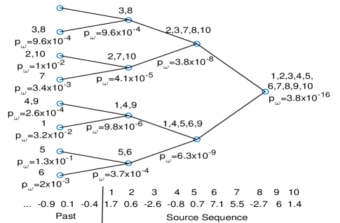
Figure 1: The source sequence of Example 2 is split up by PTW. In Example 3 the weighted probabilities are then calculated.

III-C Updating the pattern tree and complexity

Suppose a pattern tree of depth $D$ already seen the source sequence $x_{1},\cdots,x_{n-1},x_{n}$, now we want to see how complex the pattern tree evolves when the next sample $x_{n+1}$ is going to be processed. This is done by updating all the nodes in only one path of length $D$ from the root to a leaf node and this path is determined by the procedure explained in section III-A. Then the updating steps in all the $D+1$ nodes in the evolving path are: (i) updating the parameter estimation, (ii) updating predictive probabilities $P_{\eta_{i}}(x_{n+1}|\mathbf{x}_{n}^{\eta_{i}})$ and (iii) updating the weighted probabilities $P_{\omega,\eta_{i}}(x_{n+1}|\mathbf{x}_{n}^{\eta_{i}})$. The following example which is the continuation of the series of examples shows how the source sequence in Example 3 is updated for new source sample.

Example 4.

Suppose that the source has already generated the sequence of Example 2. This resulted the weighted pattern tree in Fig. 1.

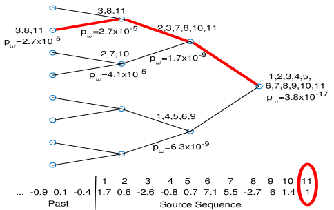
Figure 2: Updated path of the weighted pattern tree of the source sequence in Example 2 followed by a 1.

Note that by assuming a parametric model (here, a Gaussian model), there would be no more need to store all the data samples in each node; instead, only parameters should be updated and stored in the nodes.

IV Atypicality using PTW

Suppose $\mathcal{P}=\left\{P_{\boldsymbol{\theta}}\left(\mathbf{x}_{n}\right):\>\boldsymbol{\theta}\in\Theta\subset\mathcal{\mathbb{R}}^{k}\right\}$ is a family of parametric model class that can be assigned to the data. In terms of coding, Definition 1 can be stated in the following form

$$C(\mathbf{x}|\mathcal{P})-C(\mathbf{x})>0$$

Here $C(\mathbf{x}|\mathcal{P})$ is the code length of $\mathbf{x}$ encoded with the optimum coder according to the typical law (known parameters $\boldsymbol{\theta}$), and $C(\mathbf{x})$ is $x$ encoded ’in itself.’ As argued in [3], we need to put a ’header’ in atypical sequences to inform the encoder that an atypical encoder is used. We can therefore write $C(\mathbf{x})=\tau+\tilde{C}(\mathbf{x})$, where $\tau$ is the number of bits for the ’header,’ and $\tilde{C}(\mathbf{x})$ is the number of bits used for encoding the data itself. For encoding the data in itself an obvious solution is to use a universal source coder. We have therefore chosen to use the PTW algorithm.

IV-A Typical Encoding and Training

In Definition 1 we have assumed that parameters $\boldsymbol{\theta}$ of the typical model of data is exactly known, however, in many cases the parameters are not known exactly. Let us assume we are given a single long sequence $\mathbf{t}$ for training – rather than the parameters $\boldsymbol{\theta}$ in model $\mathcal{P}$ – and based on this we need to encode a sequence $\mathbf{x}$. To understand what this means, we have to realize that when $\mathbf{x}$ is encoded according to $C(\mathbf{x}|\mathcal{P})$ with a known $\mathcal{\boldsymbol{\theta}}$, the coding probabilities are fixed; they are not affected by $\mathbf{x}$. This is an important part of Definition 1 that reacts to ’outliers,’ data that does not fit the typical model. But the issue with universal source coders is that they often easily adapts to new types of data, a desirable property of a good universal source coder, but problematic in light of the above discussion. We therefore need to ’freeze’ the source coder, for example by not updating the dictionary. However, because the training data is likely incomplete as discussed above, the freezing should not be too hard. This issue is precisely described in [3] and due to page limitation we don’t go over it here, but with a simulation we show why freezing the encoder is essential in implementing atypicality: The PTW algorithm trained with a Gaussian process with $\sigma^{2}=4$ and then tested with another Gaussian source with same mean and different variance $\sigma^{2}=1$. It can be seen in Fig. 3 that the non-frozen algorithm learn the statistic and behavior of the new source; however, the codelength using frozen algorithm keeps increasing and that’s a property we are interested in.

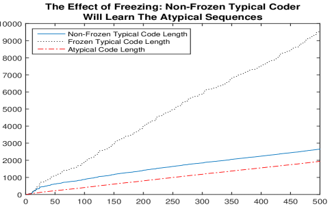
Figure 3: The importance of freezing source coding when testing for atypicality.

IV-B Atypical subsequences

Let $\mathcal{X}(n,l)=(x_{n},x_{n+1},\ldots,x_{n+l-1})$ be a subsequence of $\{\mathbf{x}_{n},n=0,\ldots,\infty\}$ that we want to test for atypicality. As mentioned earlier, the start of a sequence needs to be encoded as well as the length. Additionally the code length is minimized over the maximum depth $D$ of the context tree. The atypical code length is then given by

$$L_{A}(\mathcal{X}(n,l))= \min_{D}\left(-\log P_{\omega,\lambda}(D)+\log^{*}D\right)+\log^{*}l$$

except for the $\tau$. Here $P_{\omega,\lambda}(D)$ denotes the probability at the root of the pattern tree of depth $D$. For typical coding we use the algorithm in Section IV-A when the parameters are not known; let $L(n)$ be the codelength for the sequence $x_{0},\ldots,x_{n}$. Then we can put $L_{T}(\mathcal{X}(n,l))=L(n+l-1)-L(n)$. We need to test every subsequence of every length, that is, we need to test subsequences $\mathcal{X}(n,l)$ for every value of $n$ and $l$. For atypical coding this means that a new PTW algorithm needs to be started at every sample time. So, if the maximum sequence length is $L$, $L$ separate PTW trees need to maintained at any time. These are completely independent, so they can be run on parallel processors. The result is that for every bit of the data we calculate

$$\Delta L(n) =\min_{l}\left\{L_{A}(\mathcal{X}(n,l))-L_{T}(\mathcal{X}(n,l))\right\}$$ (6)

and we can state the atypicality criterion as $\Delta L(n)<-\tau$.

V Anomaly Detection

In [3] we have used CTW for anomaly detection in binary data and we got unique results. In order to verify the performance of our algorithm for real-valued data, here we want to use PTW as encoder in atypicality framework for same purpose.

V-A Comparison with an alternative method

In [15] authors came up with the Compression-based Dissimilarity Measure (CDM) that uses the dissimilarity measure for anomaly detection. They showed by that their proposed algorithm outperformed other methods. Here we want to compare our algorithm with CDM on a simulated data. In this experiment the training sequence is a Gaussian process with zero mean and $\sigma^{2}=4$, and the test sequence have the same statistics as the training data but with two episodes of anomalies embedded in it: a sinusoidal segment (red part in Fig. 4) and a segment of Gaussian process with zero mean and $\sigma^{2}=1$ (green part in Fig. 4). As can be verified from the figure, our PTW-based atypicality found both of the anomalies in the data; however, CDM only detected the sinusoidal pattern.

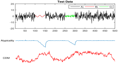
Figure 4: A comparison of two different methods. For our proposed method, the $\triangle L$ of equation (6) has been plotted. A) Gaussian process with zero mean and $\sigma^{2}=4$, exactly the same as training (typical) data, B) A sinusoidal segment C) A segment of Gaussian process with zero mean and $\sigma^{2}=1$ .

V-B Detection of Paroxysmal Atrial Fibrillation (PAF)

Paroxysmal Atrial Fibrillation (PAF) is an irregular, often rapid heart rate that commonly causes poor blood flow, which may lead to severe consequences. PhysioNet [16] has provided a database for this arrhythmia [17]. Part of this database includes 30-minute ECG records of different subjects (who have PAF) during a period that is distant from any episode of PAF. Each 30-minute record is then followed by two 5-minute record of the same subject, one of which contains an episode of PAF, and the other one has no such an episode. Fig. 5 shows HRV signal for a subject in the database.

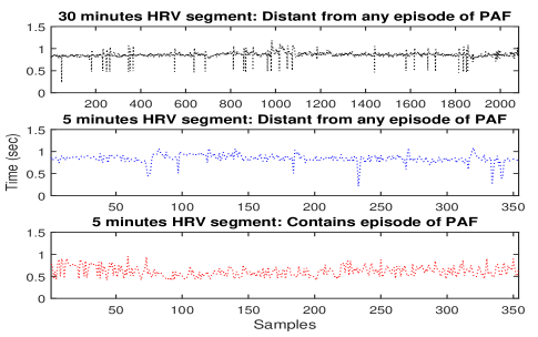
Figure 5: HRV signal of a PAF subject in the database

In our experiment, for each subject we train the PTW with HRV of 30-minute records and freeze it, then it was used as encoder for its two 5-minute segments. Our goal was to detect the 5-minute record with PAF episode, since we believed using the PTW trained on 30-minute records, smaller codelength is needed to encode the 5-minute record without PAF episode. After applying the same procedure on all the 25 subjects, we were able to detect all the 5-minute record containing PAF episode correctly, with 100 accuracy (consequently due to data structures, zero false alarm), in fact we have improved the best results of other researches on the same database about 10 percent [18, 19]. Again, as we discussed in section IV-A it verifies the importance of freezing in our notion of atypicality.

V-C Detection of anomaly in Holter Monitoring

As we mentioned earlier, the ultimate goal of atypicality is to find “unknown unknowns” in Big Data. One example can be the data that achieved by Holter Monitoring, i.e., a continuous tape recording of a patient’s ECG for 24 hours. For such a data we used the MIT-BIH Normal Sinus Rhythm Database (nsrdb) which is provided by PhysioNet [16]. Even though the subjects included in this database were found to have had no significant arrhythmias, there exist many arrhythmic beats and patterns to look for. We want to apply our algorithm to find interesting parts of the data in the dataset.

Since the data is assumed to be “Normal Sinus Rhythm,” we trained and froze our typical PTW with Gaussian process of the same mean and variance of the data. Using the process of the section IV-B, we managed to find interesting results on the dataset. As an example, we provide Fig. 6. An can be seen in the figure, for that particular data we came up with three major atypical subsequences: the first one is denotes by “S,” second one is marked with “V” and the last one as “pattern.” After looking up in the annotation file which is provided for the HRV, the “S” group corresponds to onset of some supraventricular beats and the “V” groups was the result of ventricular contraction; however, there were no label for the segment that we call “pattern” in the HRV annotations. Looking closer in the data shows existence of some repetitive patterns that was not even seen by the cardiologist who annotated the HRV data. Taking a deeper look into ECG (not HRV) annotation shows that those patterns are happening at the same time that there are either some isolated QRS-like artifact or signal quality change [16]. This shows our algorithm was able to find something that was missed by the eye of the expert who was only looking into the HRV data without considering the ECG signals; nevertheless, it could be the sign of some heart malfunction after the recording was over.

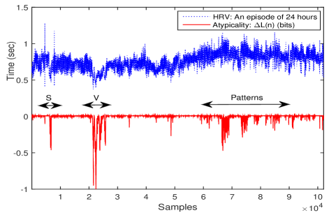
Figure 6: Atypicality using PTW for Holter Monitoring HRV: “S” stands for supraventricular arrhythmia and “V” stands for ventricular contraction

References

- [1] A. Høst-Madsen, E. Sabeti, and C. Walton, “Information theory for atypical sequences,” in IEEE Information Theory Workshop (ITW’13), Seville, Spain, 2013.
- [2] A. Host-Madsen and E. Sabeti, “Atypical information theory for real-valued data,” in 2015 IEEE International Symposium on Information Theory (ISIT). IEEE, 2015, pp. 666–670.
- [3] A. Høst-Madsen, E. Sabeti, and C. Walton, “Data discovery and anomaly detection using atypicality: Theory,” IEEE Transactions on Information Theory, submitted 2016, available at http://arxiv.org/abs/1709.03189.
- [4] A. Host-Madsen, E. Sabeti, C. Walton, and S. J. Lim-Higbie, “Universal data discovery using atypicality,” in 3rd International Workshop on Pattern Mining and Application of Big Data (BigPMA - Big Data 2016), 2016 IEEE International Conference on. IEEE, 2016.
- [5] E. Sabeti and A. Host-Madsen, “Atypicality for vector gaussian models,” in 2015 IEEE Global Conference on Signal and Information Processing (GlobalSIP). IEEE, 2015, pp. 328–332.
- [6] ——, “Atypicality for the class of exponential family,” in 2016 54rd Annual Allerton Conference on Communication, Control, and Computing (Allerton). IEEE, 2016.
- [7] ——, “How interesting images are: An atypicality approach for social networks,” in Big Data (Big Data), 2016 IEEE International Conference on. IEEE, 2016.
- [8] E. Sabeti and A. Høst-Madsen, “Data discovery and anomaly detection using atypicality: Signal processing methods,” IEEE Transactions on Signal Processing, submitted 2017, available at http://arxiv.org/abs/1709.03191.
- [9] E. Sabeti and A. Host-Madsen, “Enhanced mdl with application to atypicality,” in 2017 IEEE International Symposium on Information Theory (ISIT). IEEE, 2017.
- [10] D. Rumsfeld, Known and Unknown: A Memoir. Penguin, 2011.
- [11] J. Rissanen, “Stochastic complexity and modeling,” The Annals of Statistics, no. 3, pp. 1080–1100, Sep. 1986.
- [12] F. M. Costa T, Boccignone G, “Gaussian mixture model of heart rate variability,” PLoS ONE, no. 5, 2012.
- [13] F. M. J. Willems, Y. Shtarkov, and T. Tjalkens, “The context-tree weighting method: basic properties,” Information Theory, IEEE Transactions on, vol. 41, no. 3, pp. 653–664, 1995.
- [14] F. Willems, Y. Shtarkov, and T. Tjalkens, “Reflections on "the context tree weighting method: Basic properties",” Newsletter of the IEEE Information Theory Society, vol. 47, no. 1, 1997.
- [15] E. Keogh, S. Lonardi, and C. A. Ratanamahatana, “Towards parameter-free data mining,” in Proceedings of the tenth ACM SIGKDD international conference on Knowledge discovery and data mining. ACM, 2004, pp. 206–215.
- [16] A. L. Goldberger, L. A. N. Amaral, L. Glass, J. M. Hausdorff, P. C. Ivanov, R. G. Mark, J. E. Mietus, G. B. Moody, C.-K. Peng, and H. E. Stanley, “Physiobank, physiotoolkit, and physionet,” Circulation, vol. 101, no. 23, pp. e215–e220, 2000. [Online]. Available: http://circ.ahajournals.org/content/101/23/e215
- [17] G. Moody, A. Goldberger, S. McClennen, and S. Swiryn, “Predicting the onset of paroxysmal atrial fibrillation: The computers in cardiology challenge 2001,” in Computers in Cardiology 2001. IEEE, 2001, pp. 113–116.
- [18] E. Sabeti, M. B. Shamsollahi, and F. Afdideh, “Prediction of paroxysmal atrial fibrillation using empirical mode decomposition and rr intervals,” in Biomedical Engineering and Sciences (IECBES), 2012 IEEE EMBS Conference on. IEEE, 2012, pp. 750–754.
- [19] T. Thong, J. McNames, M. Aboy, and B. Goldstein, “Prediction of paroxysmal atrial fibrillation by analysis of atrial premature complexes,” IEEE transactions on biomedical engineering, vol. 51, no. 4, pp. 561–569, 2004.