Size–luminosity relations and UV luminosity functions at $z=6-9$
simultaneously derived from the complete Hubble Frontier Fields data

Abstract

We construct $z\sim 6-7$, 8, and 9 faint Lyman break galaxy samples (334, 61, and 37 galaxies, respectively) with accurate size measurements with the software glafic from the complete Hubble Frontier Fields cluster and parallel fields data. These are the largest samples hitherto and reach down to the faint ends of recently obtained deep luminosity functions. At faint magnitudes, however, these samples are highly incomplete for galaxies with large sizes, implying that derivation of the luminosity function sensitively depends on the intrinsic size–luminosity relation. We thus conduct simultaneous maximum-likelihood estimation of luminosity function and size–luminosity relation parameters from the observed distribution of galaxies on the size–luminosity plane with the help of a completeness map as a function of size and luminosity. At $z\sim 6-7$, we find that the intrinsic size–luminosity relation expressed as $r_{\textrm{e}}\propto L^{\beta}$ has a notably steeper slope of $\beta=0.46^{+0.08}_{-0.09}$ than those at lower redshifts, which in turn implies that the luminosity function has a relatively shallow faint-end slope of $\alpha=-1.86^{+0.17}_{-0.18}$. This steep $\beta$ can be reproduced by a simple analytical model in which smaller galaxies have lower specific angular momenta. The $\beta$ and $\alpha$ values for the $z\sim 8$ and 9 samples are consistent with those for $z\sim 6-7$ but with larger errors. For all three samples, there is a large, positive covariance between $\beta$ and $\alpha$, implying that the simultaneous determination of these two parameters is important. We also provide new strong lens mass models of Abell S1063 and Abell 370, as well as updated mass models of Abell 2744 and MACS J0416.1$-$2403.

1. Introduction

Disk sizes of galaxies at very high redshifts are important in two aspects. One is that they provide information on the formation and early evolution of galaxies. The other is that they have a significant effect on the determination of UV luminosity functions because the correction for detection incompleteness sensitively depends on size.

Concerning the first aspect, the size of galaxies is largely determined by their angular momentum (e.g., Fall & Efstathiou, 1980; Mo et al., 1998) as is the case for disk galaxies, and angular momentum is one of the fundamental parameters of galaxies as argued by Fall (1983). Romanowsky & Fall (2012) and Fall & Romanowsky (2013) have discussed galaxy formation and evolution using the specific angular momentum–mass diagram. Indeed, numerous simulations and analytical models of galaxy formation suggest that the size of galaxies changes with a redistribution of the angular momentum in them due to stellar feedback such as galactic winds (e.g., Brooks et al., 2011; Wyithe & Loeb, 2011; Brook et al., 2012; Danovich et al., 2015; Genel et al., 2015). Recently, high-resolution cosmological simulations have succeeded in increasing sizes at a fixed luminosity or stellar mass of simulated galaxies to reproduce observed sizes by incorporating stellar feedback such as galactic winds of high mass-loading factors (e.g., Brooks et al., 2011; Genel et al., 2015). The luminosity dependence of the size is also affected by stellar feedback as explained by simple analytical models. For example, Wyithe & Loeb (2011) showed that the slope of the size–luminosity relation varies depending on the dominating feedback such as energy-driven and momentum-driven feedback. Larger sizes indicate more efficient feedback, which suggests that the slope of the size–luminosity relation contains information on the dominant feedback process.

The second aspect concerning UV luminosity functions is also important because luminosity functions are determined by correcting for detection completeness, which depends on the intrinsic size distribution. For a given magnitude, galaxies with larger sizes are less likely to be detected because of their lower surface brightness. Grazian et al. (2011), based on the $z\sim 7$ analysis, have pointed out that the assumed size distribution critically alters the UV luminosity function, especially the faint-end slope.

One of the main goals of recent observational projects targeting $z\gtrsim 6$ galaxies (e.g., HUDF09/12, CANDELS, XDF, GOLDRUSH; Oesch et al., 2010b; Grogin et al., 2011; Koekemoer et al., 2011; Ellis et al., 2013; Illingworth et al., 2013; Ono et al., 2017) is to obtain the faint-end slope of luminosity functions, a key quantity for testing galaxy formation models. In addition, since $z\sim 6-10$ is the epoch of reionization and faint galaxies are thought to be major sources of ionizing photons, the abundance of faint galaxies, i.e., the faint-end slope, is important for understanding the reionization of the universe.

Recently, in order to derive luminosity functions at fainter magnitudes, deep observations combined with the power of the gravitational lensing by galaxy clusters have been conducted, such as the CLASH program (see Postman et al., 2012, for more details) and the Hubble Frontier Fields program (HFF; Lotz et al., 2017). Utilizing early-stage data from the HFF, the faint limits of luminosity functions reach as faint as UV magnitudes ($M_{\mathrm{U}V}$) of $M_{\mathrm{U}V}\sim-15.5$, $-17$, and $-17.5$ at $z\sim 6-7$, 8, and 9, respectively (Atek et al., 2014, 2015b; Ishigaki et al., 2015; McLeod et al., 2015). More recently, very faint galaxies of $M_{\mathrm{U}V}\sim-13$ at $z\sim 6-7$ have been detected using one-third of the full HFF data (Castellano et al., 2016; Livermore et al., 2017), half of them (Laporte et al., 2016), two-thirds of them (Kawamata et al., 2016; hereafter K16, Yue et al., 2017), and all of them (Ishigaki et al., 2018). However, the luminosity functions obtained in the previous studies, including those from the HFF, are still highly uncertain, especially at $M_{\mathrm{U}V}\gtrsim-18$ and $z\gtrsim 6$, because the size–luminosity relations are not determined well in that magnitude range (see our Figure 12, and Figure 2 of Bouwens et al., 2017a) owing to an insufficient number of galaxies with size measurements.

There have been a number of studies that measure sizes of bright ($M_{\mathrm{U}V}\lesssim-18$) galaxies (e.g., Ferguson et al., 2004; Bouwens et al., 2004; Curtis-Lake et al., 2016; Laporte et al., 2016; Bowler et al., 2017). At $z\sim 4$ and $5$, Huang et al. (2013) have carefully measured the size distributions of Lyman break galaxies (LBGs) with $-22.5\lesssim M_{\mathrm{U}V}\lesssim-17.5$ and find size–luminosity relations of $L\propto r_{\mathrm{e}}^{0.22-0.25}$, where $L$ and $r_{\mathrm{e}}$ are the luminosity and effective half-light radius, respectively. Oesch et al. (2010a) were among the first to measure the sizes of $z\sim 7$ and 8 galaxies with samples of 16 and five galaxies from HUDF09 (Oesch et al., 2010b) reporting that the decreasing trend of sizes with increasing redshifts continues to these redshifts. This trend has been confirmed by Ono et al. (2013) by careful measurements using the deeper imaging data from HUDF12 (Ellis et al., 2013; Koekemoer et al., 2013). With a larger sample, Grazian et al. (2012) have measured the sizes of $z\sim 7$ LBGs of moderate magnitude ($M_{\mathrm{U}V}\lesssim-18.5$). They have found that the size–luminosity relation is in the form of $L\propto r_{\mathrm{e}}^{0.5}$ at this redshift, although their size measurements may suffer from systematic biases due to their measuring method. More recently, Shibuya et al. (2015) have measured sizes for large $z\sim 6-10$ LBG samples with moderate magnitudes of $M_{\mathrm{U}V}\lesssim-18$. However, since none of the above studies has reliably determined the size–luminosity relation for $M_{\mathrm{U}V}\lesssim-18$ galaxies at $z\gtrsim 6$, a size–luminosity relation of $L\propto r_{\mathrm{e}}^{0.25}$ has been commonly adopted, given the results of Huang et al. (2013) obtained for $z\sim 4-5$. This relation is extrapolated and also applied to fainter magnitudes down to $M_{\mathrm{U}V}\sim-13$, beyond the magnitude range over which it is determined.

At faint magnitudes of $M_{\mathrm{U}V}\gtrsim-18$, Kawamata et al. (2015, hereafter K15) have used the first cluster and parallel fields data from the HFF to find that the sizes of observed faint galaxies ($-18.7\lesssim M_{\mathrm{U}V}\lesssim-16.6$) are considerably smaller than the sizes inferred from the extrapolated size–luminosity relation of $L\propto r_{\mathrm{e}}^{0.25}$. This result has subsequently been confirmed by Bouwens et al. (2017a), Laporte et al. (2016), and Bouwens et al. (2017c), who have measured the sizes of faint galaxies using four, three, and four HFF cluster fields data, respectively. In addition, Bouwens et al. (2017a) have indirectly indicated the absence of faint galaxies with large sizes using the dependence of the galaxy surface density on the lensing shear. They have concluded that the intrinsic sizes of the faintest galaxies are small, and the intrinsic size distribution assumed in the calculation of the luminosity function should be close to the observed one. This makes the faint-end slope of the luminosity function shallower. However, since none of Kawamata et al. (2015), Bouwens et al. (2017a, c), and Laporte et al. (2016) have considered an incompleteness correction due to galaxies with large sizes, the slope of the size–luminosity relation may be biased toward a steeper value. In addition, the indirect inference in Bouwens et al. (2017a) is subject to large uncertainties, which may result in weak constraints on the size distribution compared to inferences using direct size measurements.

In this paper, we provide direct size measurements of $z\sim 6-7$, 8, and 9 LBGs at $-21.6\lesssim M_{\mathrm{U}V}\lesssim-12.3$ using all six HFF cluster and parallel fields data. We show that the incompleteness effect is significant at $z\sim 6-9$ for the first time. We derive incompleteness-corrected intrinsic size–luminosity relations simultaneously with luminosity functions, which enables us to explore the correlation between these two functions. We note that we do not discuss the UV luminosity density and hence the contribution of galaxies to cosmic reionization, because the normalization parameter of UV luminosity functions is not determined in this paper.

The structure of this paper is as follows. In Section 2, we describe the data and samples, which are identical to those constructed in Ishigaki et al. (2018) but with slight changes. In Section 3, we measure the sizes of the galaxies. Our method to correct for systematic biases, which is updated from that in K15 in order to deal with the increased number of galaxies, is also described. In Section 4, for each of the three redshift ranges, we simultaneously estimate the intrinsic size–luminosity relation and the UV luminosity function from the observed distribution of galaxies on the size–luminosity plane, taking account of the incompleteness effect. The correlations between the size–luminosity and luminosity function parameters are also obtained. We discuss our findings in Section 5 and give a summary in Section 6.

Throughout this paper, we adopt a cosmology with $\Omega_{M}=0.3$, $\Omega_{\Lambda}=0.7$, and $H_{0}=70\>\mathrm{km\>s^{-1}\>Mpc^{-1}}$. Magnitudes are given in the AB system (Oke & Gunn, 1983). Galaxy sizes are measured in the physical scale.

2. Data and Sample Selection

Here we describe the data, sample selection, and obtained samples. The data and the criteria for the sample selection are the same as those in Ishigaki et al. (2018), but we remove two galaxies from their samples. Only a brief description is given in this section, and readers are referred to the above paper for further details.

2.1. HFF Mosaic Data

We use the reduced image mosaics obtained in the HFF program, which are made publicly available through the STScI website. This program targets six cluster fields, Abell 2744, MACS J0416.1$-$2403, MACS J0717.5+3745, MACS J1149.6+2223, Abell S1063, and Abell 370, and their accompanying six parallel fields. Those fields have been observed deeply with the Hubble Space Telescope using three bands of the Advanced Camera for Surveys (ACS) and four bands of the IR channel of the Wide Field Camera 3 (WFC3/IR). We utilize the v1.0 standard calibrated (i.e., without ‘self-calibration’) mosaics for the three ACS bands F435W ($B_{435}$), F606W ($V_{606}$), and F814W ($i_{814}$). For the four WFC3/IR bands F105W ($Y_{105}$), F125W ($J_{125}$), F140W ($J\!H_{140}$), and F160W ($H_{160}$), we use the v1.0 standard calibrated mosaics for the Abell 2744 parallel and MACS J0416.1$-$2403 cluster fields and v1.0 mosaics corrected for ‘time-variable sky emission’ for the other ten fields. The $5\sigma$ limiting magnitudes of the mosaics are $\sim 29$ mag on a $0\farcs 35$ diameter aperture. All the images have a pixel scale of $0\farcs 03$.

2.2. Sample Selection

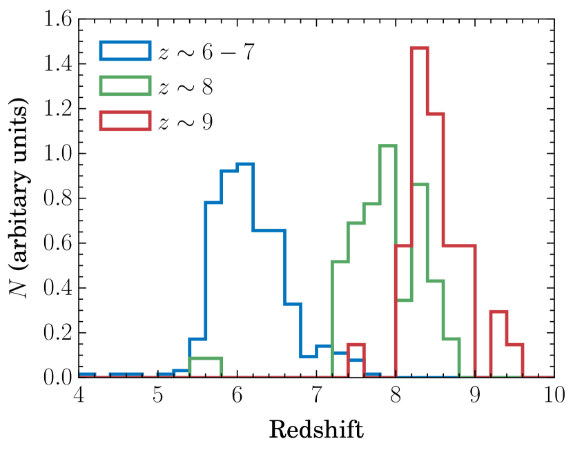
Figure 1.— Normalized distributions of the photometric redshifts of our samples for $z\sim 6-7$ (blue), 8 (green), and 9 (red).

We make two catalogs with different detection images, which are referred to as the $J\!J\!H\!H$ and $J\!H\!H$ catalogs. The detection image for the former is a $J_{125}$, $J\!H_{140}$, and $H_{160}$ combined image, and for the latter it is a $J\!H_{140}$ and $H_{160}$ combined image; these are created using SWarp v2.38.0 (Bertin et al., 2002) together with their weight maps. To make the catalogs, we run SExtractor v2.8.6 (Bertin & Arnouts, 1996) on the seven bands’ images using the detection images. The photometric redshifts of galaxies in these catalogs are estimated using BPZ v1.99.3 (Benítez, 2000). From the catalogs, we select $i$-, $Y$-, and $Y\!J$-dropout galaxies using the Lyman break technique. For $i$- and $Y$-dropout selections, we use the $J\!J\!H\!H$ catalog and for $Y\!J$-dropout selection, we use the $J\!H\!H$ catalog. For $i$-dropouts or $z\sim 6-7$ galaxies, we use the criteria of

$$i_{814}-Y_{105} >0.8,$$ (1)

$$Y_{105}-J_{125} <0.8,$$ (2)

$$i_{814}-Y_{105} >2(Y_{105}-J_{125})+0.6,$$ (3)

for $Y$-dropouts or $z\sim 8$ galaxies,

$$Y_{105}-J_{125} >0.5,$$ (4)

$$J_{125}-J\!H_{140} <0.5,$$ (5)

$$Y_{105}-J_{125} >0.4+1.6(J_{125}-J\!H_{140}),$$ (6)

and for $Y\!J$-dropouts or $z\sim 9$ galaxies,

$$(Y_{105}+J_{125})/2-J\!H_{140} >0.75,$$ (7)

$$(Y_{105}+J_{125})/2-J\!H_{140}$$

$$>0.75 +0.8(J\!H_{140}-H_{160}),$$ (8)

$$J_{125}-H_{160} <1.15,$$ (9)

$$J\!H_{140}-H_{160} <0.6.$$ (10)

For $i$-dropouts, we use additional signal-to-noise ratio constraints that require objects not to be detected at $>2\sigma$ levels in both the $B_{435}$- and $V_{606}$-band images or in a $B_{435}$ + $V_{606}$ stacked image. Detections at $>5\sigma$ levels are also required in both the $Y_{105}$- and $J_{125}$-band images. For a conservative selection, $i_{814}$ magnitudes are replaced by the $i_{814}$ $2\sigma$ limiting magnitude if the signal is below that level. For $Y$-dropouts, objects are required to be detected at $>2\sigma$ levels in none of the $B_{435}$-, $V_{606}$-, and $i_{814}$-band images. In addition, detections at $>5\sigma$ levels are required in all of the $J_{125}$-, $J\!H_{140}$-, and $H_{160}$-band images. For $Y\!J$-dropouts, objects are required to be detected at $>2\sigma$ levels in none of the $B_{435}$-, $V_{606}$-, and $i_{814}$-band images. In addition, detections at $>3\sigma$ levels are required in all of the $J\!H_{140}$- and $H_{160}$-band images and at $>3.5\sigma$ levels in at least one of these band images. Magnitudes of $Y_{105}$ and $J_{125}$ are replaced by their $0.9\sigma$ limiting magnitudes if the signal is below that level. Finally, we remove objects whose pseudo-$\chi^{2}$ is larger than 2.8, with $\chi^{2}=\sum_{i}\mathrm{SGN}(f_{i})(f_{i}/\sigma_{i})^{2}$, where the summation runs over all the ACS bands. Here $f_{i}$ and $\sigma_{i}$ are the flux density and its uncertainty in the $i$-th band image, respectively, and $\mathrm{SGN}(f_{i})$ is the sign function, whose definition is $\mathrm{SGN}(x)=1$ if $x>0$, $\mathrm{SGN}(x)=0$ if $x=0$, and $\mathrm{SGN}(x)=-1$ if $x<0$. The selected dropout galaxies are presented in Tables 4–6 in Ishigaki et al. (2018).

From the Ishigaki et al. (2018) samples, we remove a $Y$-dropout galaxy, HFF6P-1733-6559, and a $Y\!J$-dropout galaxy, HFF6P-1732-6562, in the Abell 370 parallel field, because they appear to be spurious sources by visual inspection. These are indeed the same object meeting both the $Y$- and $Y\!J$-dropout selections. As a result, the total numbers of the selected galaxies are 350, 64, and 39 for $i$-, $Y$-, and $Y\!J$-dropouts, respectively. Their photometric redshift distributions are shown in Figure 1. The averages of the reliable ($z>4$) photometric redshifts of the $i$-, $Y$-, and $Y\!J$-dropouts are $z=6.2$, $7.8$, and $8.5$, respectively. Therefore, we use $z=6$, $8$, and $9$ in the calculation of the sizes, magnitudes, and magnification factors for $i$-, $Y$-, and $Y\!J$-dropouts, respectively. Fixing the redshift to these values does not cause any systematic errors in the following results.

3. Size and Magnitude Measurements

3.1. Two-dimensional Profile Fitting

In this subsection, we estimate lensing-corrected, i.e., intrinsic, sizes and magnitudes of the dropout galaxies.

The lensing effects are calculated using the software glafic v1.2.7 (Oguri, 2010). For the mass distributions of Abell 2744 and MACS J0416.1$-$2403, we use our version 4 mass models updated to reflect the latest MUSE observations by Mahler et al. (2018) and Caminha et al. (2017), respectively. For MACS J0717.5+3745 and MACS J1149.6+2223, we use our version 3 mass models constructed in K16. For Abell S1063 and Abell 370, we newly construct version 4 mass models following the method established in K16. Modeling details about the four version 4 mass models are described in Appendix A. All of the mass models are available on the Space Telescope Science Institute website. The uncertainty in each magnification factor is calculated from ten-thousand models sampled from a Markov chain Monte Carlo (MCMC) chain (see Section 3.2). This uncertainty is smaller than the scatter in magnification factors among all modeling teams’ models. The typical scatters are $30\%$ at $\mu\sim 2$ and $70\%$ at $\mu\sim 40$ as reported in Priewe et al. (2017), who have conducted a thorough comparison between the mass maps of Abell 2744 and MACS J0416.1$-$2403 by all modeling teams (see also Meneghetti et al., 2017). The smaller uncertainties in our models are due to limited flexibilities inherent in parametric modeling methods, while the predicted magnification factors are consistent with those by the other teams (see Figures 10–11 and 12–13 in Priewe et al., 2017).

The method to measure intrinsic sizes and magnitudes is identical to that in K15. However, while the measurements in K15 were conducted only for bright galaxies, here we deal with all the galaxies in the samples. We fit a Sérsic profile to a galaxy image in an $8\farcs 4\times 8\farcs 4$ cutout image using a two-dimensional fitting algorithm conducted by the command optimize in glafic, which simultaneously corrects for the lensing and point-spread function (PSF) effects. In order to correct for the lensing effects, an ellipsoidal Sérsic profile on the source plane is lensed onto the image plane, and the galaxy image is fitted with the lensing-distorted Sérsic profile. In order to correct for the PSF effects, the lensing-distorted Sérsic profile is convolved with an average stellar image on the image plane, which is generated by stacking $5$–$20$ stars found in each field. The Sérsic profile is defined as

$$\Sigma(r)=\Sigma_{0}\exp\left[-b_{n}\left(\frac{r}{r_{\rm e}}\right)^{1/n}\right],$$ (11)

where $\Sigma(r)$, $\Sigma_{0}$, $b_{n}$, $r_{\rm e}$, and $n$ represent the surface brightness profile, surface brightness at $r=0$, parameter to convert the scale radius to the half-light radius, half-light radius, and Sérsic index, respectively. The ellipticity $e$ and position angle are introduced by a simple variable transformation (see Oguri, 2010, for details). In what follows, $r_{\rm e}$ means the circularized half-light radius, $r^{\rm maj}_{\rm e}\sqrt{1-e}$, where $r^{\rm maj}_{\rm e}$ is the radius along the major axis. The magnitude is calculated from $r_{\rm e}$ and $\Sigma_{0}$. During the fitting, the Sérsic index is fixed to $n=1$ and the maximum ellipticity is set to 0.9. A uniform sky background is assumed, and the normalization is optimized at the same time. When nearby objects may introduce any bias to the fitting result, we mask these objects or add additional profiles to fit the nearby objects simultaneously. The fittings are conducted using the $Y\!J\!J\!H$, $J\!J\!H\!H$, and $J\!H\!H$ combined images at $z\sim 6-7$, 8, and 9, respectively. Although we have already constructed size samples in K15 from the Abell 2744 cluster and parallel fields, we conduct the fittings again because there are updates on the mass map of the cluster. The obtained morphological properties and magnitudes are presented in Tables 13–15 in Appendix B. The fitting results for galaxies fainter than $-18$ mag are also graphically shown in Figures 18 and 19 in Appendix B.

3.2. Error Estimations

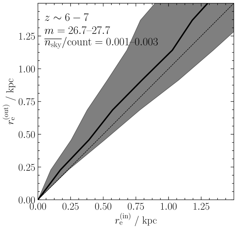
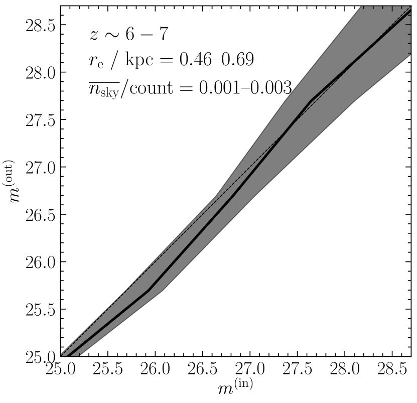
Figure 2.— Examples of the Monte Carlo simulations to estimate the systematic and random errors in size and magnitude measurements. The top panel shows the median and $1\sigma$ distribution of output radii as a function of input radius for galaxies with an apparent magnitude of $m/\mathrm{mag}=26.7$–$27.7$ and for a sky value of $\overline{n_{\mathrm{sky}}}/\mathrm{count}=0.001$–$0.003$. The bottom panel shows the median and $1\sigma$ distribution of output magnitudes as a function of input magnitude for galaxies with $r_{\mathrm{e}}/\mathrm{kpc}=0.46$–$0.69$ and for a sky value of $\overline{n_{\mathrm{sky}}}/\mathrm{count}=0.001$–$0.003$.

In this subsection, we evaluate errors in the measured sizes and magnitudes following the method in K15, but in a more efficient way. We consider two sources of errors: errors in the fitting procedure and errors in the mass map.

There are two types of errors in the fitting procedure. One is a systematic bias, by which the sizes and magnitudes of larger (smaller) galaxies are underestimated (overestimated). The other is a random error, which arises from random sky noise that disperses the estimated size and magnitude. In order to estimate these errors, we conduct Monte Carlo simulations, in which we bury simulated galaxies in a real image and perform the same fitting procedure as for real dropout galaxies. Since these systematic and random errors are primarily dependent on the galaxy apparent magnitude, apparent radius, and sky value in the vicinity, we estimate the two errors as a function of the three parameters. We use the Abell 2744 cluster field image for this derivation and apply the relation to all twelve fields. In detail, first, we select a random position in the image and bury an $n=1$ Sérsic profile, whose magnitude, radius, ellipticity, and position angle are chosen randomly. Second, we conduct the same procedure on this pseudo-galaxy as for real galaxies. We repeat these two processes until we obtain a sufficient number of measurements in each parameter bin. Third, for each real dropout galaxy, we choose a set of simulated galaxies whose apparent magnitudes, apparent radii, and sky values in the vicinity are close to those of the dropout galaxy. Using the intrinsic magnitudes and radii of the simulated galaxies in this set, we estimate the random errors and correct for the systematic errors in size and magnitude. Examples of the Monte Carlo simulations are presented in Figure 2.

Systematic errors in mass maps also affect measurement results. Since the apparent magnitudes and sizes of lensed galaxies are converted into intrinsic values using mass maps, an overestimate of the magnification factor results in an underestimate of the intrinsic sizes and magnitudes, and vice versa. In order to estimate the errors in magnification, we generate an MCMC chain of the mass model parameters using the command mcmc in glafic. From ten-thousand samples in the chain, we estimate the error in magnification factor at the positions of each dropout galaxy with the mcmc_calcim command. For each cluster, one hundred mass maps generated from randomly selected MCMC samples are available on the Space Telescope Science Institute website.

The random errors in size and magnitude due to the fitting procedure and random errors in magnification factor are presented in Tables 13–15.

4. Size–luminosity Distributions at $z\sim 6-9$

In this section, we first present the distribution of our galaxies on the size–luminosity plane. Then, detection incompleteness is calculated as a function of absolute magnitude and size for each field and redshift range. Finally, we use these incompleteness maps on the size–luminosity plane to simultaneously derive intrinsic size–luminosity relations and luminosity functions for the first time at these redshift ranges.

4.1. Galaxy Distribution on the Size–luminosity Plane

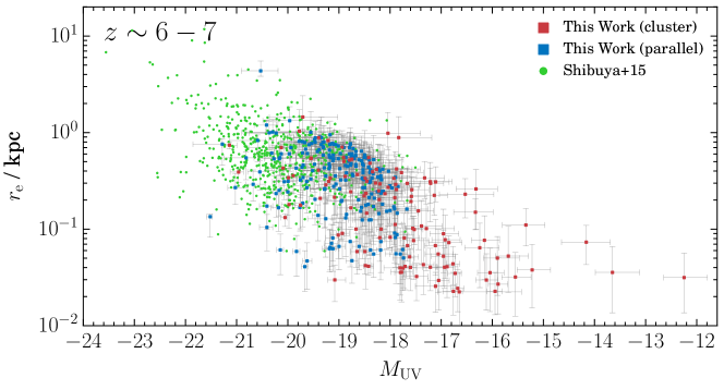
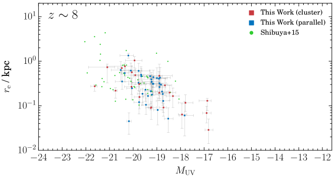
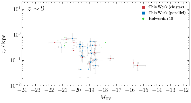
Figure 3.— Galaxy distributions on the size–luminosity plane at $z\sim 6-7$ (top), $8$ (middle), and $9$ (bottom). The red and blue points represent our galaxies from the cluster fields and parallel fields, respectively. The green points represent galaxies at $z\sim 6-7$ and $z\sim 8$ in Shibuya et al. (2015) (top and middle, respectively) and at $z\sim 9$ in Holwerda et al. (2015) (bottom).

Table 1Number of $M_{\mathrm{UV}}\gtrsim-18$ galaxies in the present and previous samples

References	$z\sim 6-7$	$z\sim 8$	$z\sim 9$	Data
This work	91 (350)	7 (64)	3 (39)	Six HFF cluster and parallel fields
Ono et al. (2013)	0 (9)	0 (6)	—	HUDF12
Holwerda et al. (2015)	—	—	1 (8)	XDF and CANDELS
Kawamata et al. (2015)	4 (31)	0 (8)	—	First HFF cluster and parallel fields
Shibuya et al. (2015)	$7+1$ $(422+173)\tablenotemark{a}$	0 (46)	—	CANDELS, HUDF09/12, and first two HFF parallel fields
Bouwens et al. (2017a)	47 (76)	—	—	First two HFF cluster fields

Note. — The number of galaxies in the full sample is shown in parentheses.

Figure 3 shows the size–luminosity distributions of our galaxies at $z\sim 6-7$, $8$, and $9$, together with those from previous studies that adopt two-dimensional profile fittings in size measurements. The error bars include the errors in the fitting process and our mass maps. Our samples occupy either the same regions as the previous samples or their reasonable extrapolations toward much fainter magnitudes.

As summarized in Tables 13–15, some galaxies are multiply imaged on the image plane. The physical parameters of these galaxies are calculated by averaging over the multiple images. The numbers of independent galaxies with size measurements are thus reduced to 334, 61, and 37 at $z\sim 6-7$, 8, and 9, respectively. Among them, the numbers of faint ($M_{\mathrm{U}V}\gtrsim-18$) galaxies are 83, six, and three, respectively. These numbers should be compared only with those from previous studies that adopt parametric size measurements such as GALFIT (Peng et al., 2002, 2010), not with those based on nonparametric methods such as “curve-of-growth.” This is because these two methods rely on different assumptions, which may introduce different biases and therefore make comparisons of the results difficult. At faint magnitude ranges, as investigated in this work, previous studies that adopt parametric size measurements are Ono et al. (2013), K15, Holwerda et al. (2015), Shibuya et al. (2015), and Bouwens et al. (2017a) (see also Oesch et al., 2010a). The numbers of galaxies in our samples and in the previous studies are presented in Table 1. For $z\sim 6-7$ and $9$, the addition of our samples increases the numbers of faint ($M_{\mathrm{U}V}\gtrsim-18$) galaxies with size measurements about $2.5$ and $4$ times, respectively. For $z\sim 8$, our sample is the first that contains faint galaxies with size measurements. The faintest objects among the previous samples have $M_{\mathrm{UV}}\simeq-14.48$ (Bouwens et al., 2017a), $-18.1$ (Shibuya et al., 2015), and $-17.8$ (Holwerda et al., 2015) at $z\sim 6-7$, 8, and 9, respectively. We push the faint limits down to $M_{\mathrm{UV}}\simeq-12.3$, $-16.8$, and $-15.4$ at $z\sim 6-7$, $8$, and 9, respectively.

4.2. Completeness Estimation

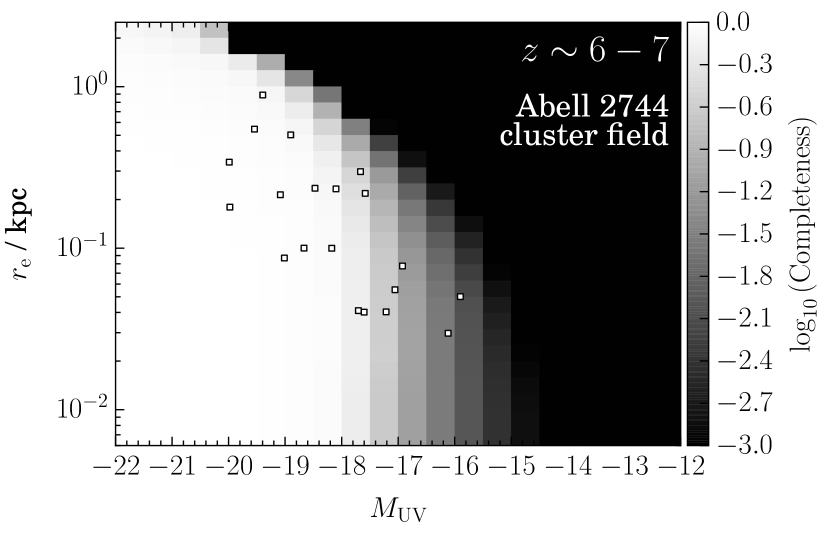
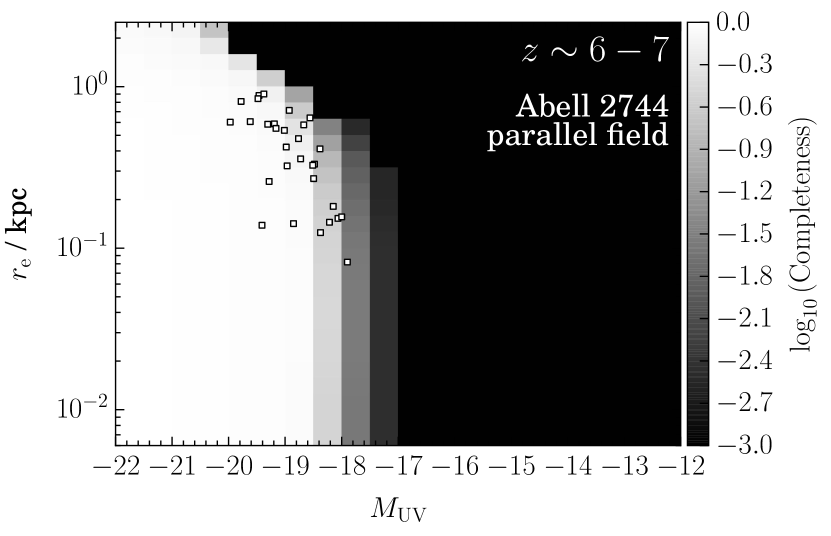
Figure 4.— Detection completeness at $z\sim 6-7$ as a function of absolute magnitude and size for the Abell 2744 cluster (top) and parallel (bottom) fields, shown on a logarithmic scale. Galaxies detected in each field are plotted with squares.

For a given total magnitude, galaxies with larger sizes are less likely to be detected in observations because of their low surface brightnesses. Since this effect is more prominent for fainter objects, observed size–luminosity relations can become significantly steeper than intrinsic ones. We conduct the following Monte Carlo simulations to calculate detection completeness as a function of absolute magnitude and size. The detection completeness is defined as the fraction of galaxies that are detected and pass the dropout selection described in Section 2.2. (1) We select random positions uniformly on the source plane. (2) For each position, we generate an artificial galaxy with a certain size and magnitude and place it, taking the lensing and PSF effects into account, into the combined image, which is used as the detection image in the catalog construction. The galaxy is modeled with a Sérsic profile of the index $n=1$. The ellipticity is randomly chosen from a uniform distribution between 0 and 0.9. (3) We run SExtractor on the image with artificial galaxies and calculate the fraction of artificial galaxies that are detected by SExtractor and bright enough to meet the criteria of dropout selection. (4) We repeat steps (1)–(3), changing the size and magnitude of artificial galaxies. It should be noted that we do not assume any specific spectral energy distribution (SED) shape. This is because, primarily, the completeness is not dependent on the SED shape but only on size and magnitude. As an example, the obtained completeness maps at $z\sim 6-7$ in the Abell 2744 cluster and parallel fields are shown in Figure 4. Note that although faint galaxies are bright enough to be detected if highly magnified, their completeness is significantly low because they rarely fall onto highly magnified regions.

As seen in Figure 5, the observed size–luminosity distributions can be significantly deformed by incompleteness, which depends on size and luminosity. We discuss the impact of incompleteness on the estimation of the intrinsic size–luminosity relations in Section 5.1. In the cluster fields, even galaxies fainter than $\sim-18$ mag are detected, but with low completeness. For example, at $M_{\mathrm{UV}}=-16$, only those with $r_{\mathrm{e}}<0.1$ kpc are included in the samples. This means that while the HFF has opened a window to faint galaxies, it is open only to very small objects. On the other hand, galaxies detected in the parallel fields are limited to $\sim-18$ mag, but with a relatively high completeness over a wide size range because completeness drops sharply at $M_{\mathrm{UV}}\sim-18$. Therefore, the cluster fields require a more careful consideration of incompleteness effects.

4.3. Maximum-likelihood Estimation
of the Intrinsic Size–luminosity Distribution

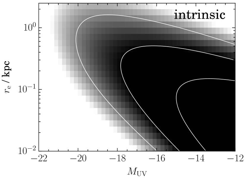
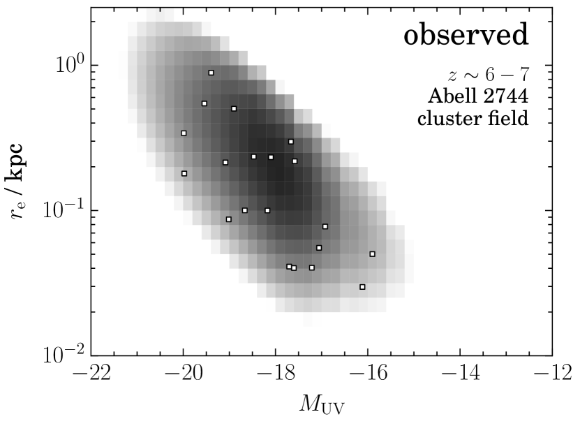
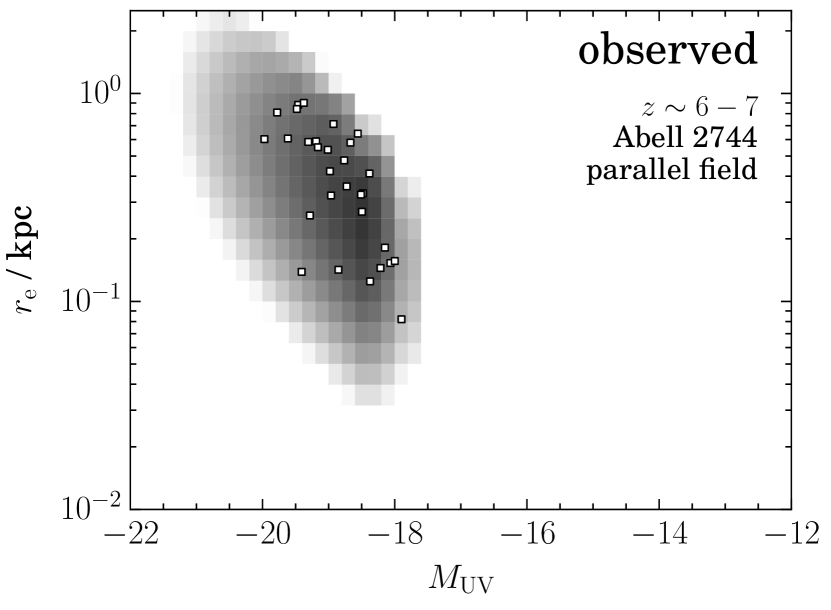
Figure 5.— Bivariate probability distributions of $z\sim 6-7$ galaxies on the size–luminosity plane shown on a logarithmic scale. The top panel shows the intrinsic distribution with an arbitrary normalization. The contour levels are logarithmically equidistant with 1 dex steps. The middle and bottom panels are for the observed distributions in the Abell 2744 cluster and parallel fields, respectively, calculated by multiplying the intrinsic distribution by the completeness map for each field. Galaxies detected in each field are shown with squares in the lower two panels. The parameters of the intrinsic bivariate distribution presented here are the best-fit parameters obtained in Section 4.3.

In this subsection, we obtain for each of the three redshift ranges the incompleteness-corrected or intrinsic bivariate size–luminosity distribution of galaxies, which is a product of the intrinsic size–luminosity relation and the luminosity function. We model the size–luminosity relation by a log-normal distribution with three free parameters while modeling the luminosity function by a Schechter function with two free parameters; the total number of free parameters is thus five. Then, by multiplying the intrinsic distribution by the incompleteness map, we model the observed size–luminosity distribution of galaxies. Maximum-likelihood estimation (MLE) is used to obtain the best-fit values of these parameters that best reproduce the observed bivariate distribution.

This bivariate method has been exploited in de Jong & Lacey (2000) and Huang et al. (2013) to simultaneously derive the size–luminosity relation and UV luminosity function for local spiral galaxies and LBGs at $z\sim 4-5$, respectively. A similar method has also been adopted in Schmidt et al. (2014a). This method has two advantages over binning methods conventionally adopted as described in Schmidt et al. (2014a); one is that no information is lost because data are not binned, and the other is that photometric errors in magnitude are also considered. In addition, by determining the size–luminosity relation and luminosity function simultaneously, we are able to evaluate the degeneracy between those two relations. Furthermore, in most previous studies, size–luminosity relations have been determined to minimize the residuals in size, which is equivalent to MLE that assumes observed galaxies have a flat distribution in luminosity. On the other hand, our method correctly derives the size–luminosity relation and, consequently, the luminosity function because the luminosity distribution is also modeled using luminosity functions.

The probability density function (PDF) of the intrinsic galaxy distribution on the size–luminosity plane $\Psi(r_{\rm e},M_{\mathrm{UV}})$ is modeled as

$$\Psi(r_{\rm e},M_{\mathrm{UV}};r_{0},\sigma,\beta,M^{*},\alpha)$$

$$=P(r_{\rm e},M_{\mathrm{UV}};r_{0},\sigma,\beta)\,\phi(M_{\mathrm{UV}};M^{*},\alpha),$$ (12)

where $P(r_{\rm e},M_{\mathrm{UV}})$ is the PDF of size and $\phi(M_{\mathrm{UV}})$ is that of luminosity. As $P(r_{\rm e},M_{\mathrm{UV}})$, we adopt a log-normal distribution described as

$$P(r_{\rm e},M_{\mathrm{UV}};r_{0},\sigma,\beta)=\frac{1}{\sigma r_{\rm e}\sqrt{2\pi}}\exp\left[-\frac{\ln^{2}(r_{\rm e}/\overline{r_{\rm e}})}{2\sigma^{2}}\right],$$ (13)

where

$$\overline{r_{\rm e}}(L)=r_{0}\left(\frac{L}{L_{0}}\right)^{\beta},$$ (14)

and $r_{0}$, $\sigma$, $\beta$, and $L_{0}$ are the modal radius at $M_{\mathrm{UV}}=-21$, width of the log-normal distribution, slope of the size–luminosity relation, and luminosity corresponding to $M_{\mathrm{UV}}=-21$, respectively. As $\phi(M_{\mathrm{UV}})$, we adopt a Schechter function described as

$$\phi(M_{\mathrm{UV}};M^{*},\alpha)$$

$$=10^{-0.4(\alpha+1)(M_{\mathrm{UV}}-M^{*})}\exp{\left[-10^{-0.4(M_{\mathrm{UV}}-M^{*})}\right]},$$ (15)

where $M^{*}$ and $\alpha$ are the characteristic magnitude and power-law slope at the faint end. Note that we do not determine the normalization parameter $\phi_{*}$ of the Schechter function because we are interested not in the absolute number of galaxies but only in their relative distribution on the size–luminosity plane.

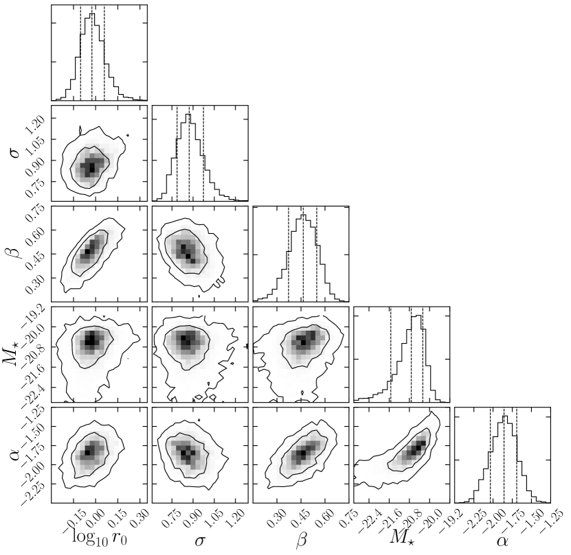
Figure 6.— Two-dimensional projections of the MCMC samples at $z\sim 6-7$. The inner and outer contours represent $68\%$ and $95\%$ confidence intervals. The three vertical dashed lines on the histograms show the 16th, 50th, and 84th percentiles. Plotted using the corner.py module (Foreman-Mackey, 2016).

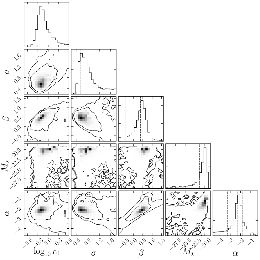
Figure 7.— Same as Figure 6 but for $z\sim 8$.

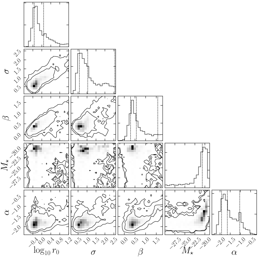
Figure 8.— Same as Figure 6 but for $z\sim 9$.

Table 2Best-fit parameters of size–luminosity relations and luminosity functions

References	$r_{0}/\mathrm{kpc}$	$\sigma$	$\beta$	$M^{*}$	$\alpha$
$z\sim 6-7$
This work	$0.94^{+0.20}_{-0.15}$	$0.87^{+0.10}_{-0.09}$	$0.46^{+0.08}_{-0.09}$	$-20.73^{+0.46}_{-0.81}$	$-1.86^{+0.17}_{-0.18}$
This work (mode)	$0.94$	$0.86$	$0.44$	$-20.56$	$-1.86$
This work (LF fixed)	$0.95^{+0.18}_{-0.14}$	$0.86^{+0.09}_{-0.07}$	$0.47^{+0.06}_{-0.06}$	$[-20.73]$	$[-1.86]$
This work (apparent)	$0.75$	$0.66$	$0.52$	—	—
Atek et al. (2015a)	$[0.81]$	$[0.90]$	$[0.25]$	$-20.89^{+0.60}_{-0.72}$	$-2.04^{+0.17}_{-0.13}$
Bouwens et al. (2015)	—	—	$[\sim 0.25]$	$-20.94^{+0.20}_{-0.20}$	$-1.87^{+0.10}_{-0.10}$
Laporte et al. (2016)	$[0.81]$	$[0.90]$	$[0]$	$-20.33^{+0.37}_{-0.47}$	$-1.91^{+0.26}_{-0.27}$
Livermore et al. (2017)	$[0.5]$	$[0]$	$[0]$	$-20.819^{+0.044}_{-0.034}\ {}^{+0.001}_{-0.031}$	$-2.10^{+0.03}_{-0.03}\ {}^{+0.07}_{-0.01}$
Ishigaki et al. (2018)	—	—	$[\sim 0.25]$	$-20.89^{+0.17}_{-0.13}$	$-2.15^{+0.08}_{-0.06}$
Bouwens et al. (2017b)	$[0.80]$	$[0.69]$	$[0.27]$	$[-20.94]$	$-1.92^{+0.04}_{-0.04}$
$z\sim 8$
This work	$0.81^{+5.28}_{-0.26}$	$0.80^{+1.07}_{-0.26}$	$0.38^{+0.28}_{-0.78}$	$-151.98^{+130.60}_{-314.19}$	$-2.26^{+0.49}_{-0.99}$
This work (mode)	$0.58$	$0.56$	$0.44$	$-19.95$	$-2.14$
This work ($M_{*}$ fixed)	$0.75^{+0.53}_{-0.16}$	$0.65^{+0.35}_{-0.14}$	$0.50^{+0.16}_{-0.21}$	$[-20.73]$	$-1.80^{+0.22}_{-0.30}$
This work (LF fixed)	$0.69^{+0.24}_{-0.14}$	$0.62^{+0.18}_{-0.12}$	$0.49^{+0.13}_{-0.14}$	$[-20.73]$	$[-1.86]$
This work (apparent)	$0.57$	$0.48$	$0.52$	—	—
Bouwens et al. (2015)	—	—	$[\sim 0.25]$	$-20.63^{+0.36}_{-0.36}$	$-2.02^{+0.23}_{-0.23}$
Laporte et al. (2016)	$[0.81]$	$[0.90]$	$[0]$	$-20.32^{+0.49}_{-0.26}$	$-1.95^{+0.43}_{-0.40}$
Livermore et al. (2017)	$[0.5]$	$[0]$	$[0]$	$-20.742^{+0.195}_{-0.152}\ {}^{+0.006}_{-0.014}$	$-2.02^{+0.08}_{-0.07}\ {}^{+0.01}_{-0.03}$
Ishigaki et al. (2018)	—	—	$[\sim 0.25]$	$-20.35^{+0.20}_{-0.30}$	$-1.96^{+0.18}_{-0.15}$
$z\sim 9$
This work	$1.20^{+367.64}_{-0.74}$	$1.04^{+1.52}_{-0.46}$	$0.56^{+1.01}_{-0.27}$	$-82.74^{+62.10}_{-763.40}$	$-1.64^{+0.61}_{-0.28}$
This work (mode)	$0.42$	$0.54$	$0.40$	$-19.80$	$-1.82$
This work ($M_{*}$ fixed)	$0.59^{+0.61}_{-0.16}$	$0.69^{+0.40}_{-0.20}$	$0.42^{+0.17}_{-0.15}$	$[-20.73]$	$-1.59^{+0.19}_{-0.18}$
This work (LF fixed)	$0.53^{+0.27}_{-0.13}$	$0.68^{+0.27}_{-0.18}$	$0.34^{+0.13}_{-0.14}$	$[-20.73]$	$[-1.86]$
This work (apparent)	$0.43$	$0.47$	$0.39$	—	—
Oesch et al. (2013)	—	—	—	$-18.8^{+0.3}_{-0.3}$	$[-1.73]$
Laporte et al. (2016)	$[0.81]$	$[0.90]$	$[0]$	$[-20.45]$	$-2.17^{+0.41}_{-0.43}$
Ishigaki et al. (2018)	—	—	$[\sim 0.25]$	$-51.39^{+18.51}_{-44.73}$	$-2.22^{+0.26}_{-0.17}$

Note. — Numbers in square brackets are fixed during the fitting.

The observed size–luminosity distribution $\Psi^{\prime}$ in the $i$-th field is modeled by multiplying the parameterized intrinsic size–luminosity distribution and the completeness map in that field $\mathcal{C}_{i}$ obtained in Section 4.2,

$$\Psi^{\prime}_{i}(r_{\mathrm{e}},M_{\mathrm{UV}};r_{0},\sigma,\beta,M^{*},\alpha)\equiv\mathcal{N}_{i}\,\Psi(r_{\mathrm{e}},M_{\mathrm{UV}})\,\mathcal{C}_{i}(r_{\mathrm{e}},M_{\mathrm{UV}}),$$ (16)

where $\mathcal{N}_{i}$ is the normalization parameter to make the volume unity. The probability that a galaxy with $(r_{\mathrm{e}},r_{\mathrm{e}}+dr_{\mathrm{e}})$ and $(M_{\mathrm{UV}},M_{\mathrm{UV}}+dM_{\mathrm{UV}})$ is found is $\Psi^{\prime}(r_{\mathrm{e}},M_{\mathrm{UV}})\ dr_{\mathrm{e}}\ dM_{\mathrm{UV}}$. In order to calculate the probability of the $j$-th galaxy in the $i$-th field $f_{i,j}$ considering the observed errors in size and magnitude, we convolve the modeled observed size–luminosity distribution $\Psi^{\prime}$ with a two-dimensional gaussian centered on the observed size and magnitude, whose variances are equal to their observed errors,

$$f_{i,j}=\int\,dr^{\prime}_{\mathrm{e}}\,dM^{\prime}_{\mathrm{UV}}$$

$$\times\Psi^{\prime}_{i}(r^{\prime}_{\mathrm{e}},M^{\prime}_{\mathrm{UV}})\,g(r^{\prime}_{\mathrm{e}},M^{\prime}_{\mathrm{UV}};r_{\mathrm{e},j},M_{\mathrm{UV},j},\delta r_{\mathrm{e},j},\delta M_{\mathrm{UV},j}),$$ (17)

where $g(r^{\prime}_{\mathrm{e}},M^{\prime}_{\mathrm{UV}};r_{\mathrm{e},j},M_{\mathrm{UV},j},\delta r_{\mathrm{e},j},\delta M_{\mathrm{UV},j})$ is a gaussian function whose peak is at the observed size and magnitude ($r_{\mathrm{e},j},M_{\mathrm{UV},j}$) and the variances are equal to their observed errors $(\delta r_{\mathrm{e},j},\delta M_{\mathrm{UV},j})$. The likelihood in the $i$-th field $\mathcal{L}_{i}$ is given by

$$\mathcal{L}_{i}(r_{0},\sigma,\beta,M^{*},\alpha)=\prod_{j}f_{i,j}(r_{0},\sigma,\beta,M^{*},\alpha).$$ (18)

The total likelihood $\mathcal{L}$ is the product of the likelihood in each field,

$$\mathcal{L}\equiv\prod_{i}\mathcal{L}_{i}.$$ (19)

We use the MCMC procedure to estimate the best-fit values and uncertainties for the five parameters and the degeneracy between them. We assume flat priors on all five parameters. Note that we do not use the galaxies HFF5P-1940-3315 at $z\sim 6-7$ and HFF5P-2129-2064 at $z\sim 8$ in the Abell S1063 parallel field because they are outliers. For the MCMC sampling, we use the public software emcee (Foreman-Mackey et al., 2013). The MCMC results are shown in Table 2 and Figures 6–8. As an example, the obtained intrinsic bivariate size–luminosity distribution at $z\sim 6-7$ is presented in the top panel of Figure 5.

5. Discussion

In this section, we first discuss the intrinsic size–luminosity relations and luminosity functions at $z\sim 6-9$. Second, we construct a model to reproduce the steep size–luminosity relation at $z\sim 6-7$ using the result of the abundance matching in Behroozi et al. (2013). Third, we show that there are large uncertainties in the $z>6$ luminosity functions derived in previous studies because of a large variance in the assumed size–luminosity relations and that those uncertainties are greatly reduced at least for $z\sim 6-7$ by using the size–luminosity relation obtained in this work. Finally, we discuss the redshift evolution of size.

5.1. The Intrinsic Size–luminosity Relation
and Luminosity Function at $z\sim 6-7$

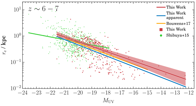
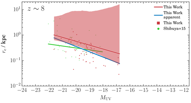
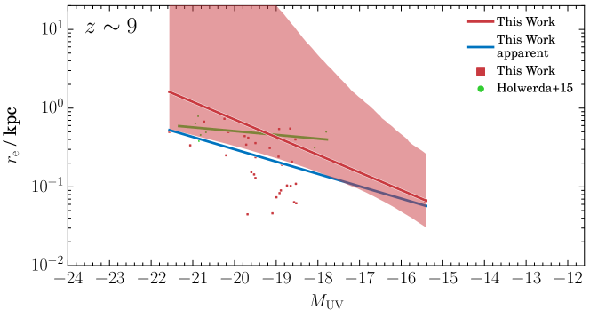
Figure 9.— Galaxy distributions on the size–luminosity plane at $z\sim 6-7$ (top), 8 (middle), and 9 (bottom), respectively. The red and green points represent, respectively, our galaxies and those from previous studies (Shibuya et al. 2015, for $z\sim 6-7$ and $8$; Holwerda et al. 2015 for $z\sim 9$). The red and blue solid lines represent the size–luminosity relations by the completeness-corrected and completeness-uncorrected fittings to our samples, respectively. The $1\sigma$ distribution of the completeness-corrected size–luminosity relation is shown by the red shaded region. While the green solid lines show the best-fit power laws obtained by Shibuya et al. (2015) and Holwerda et al. (2015), the orange solid line is for the result obtained by Bouwens et al. (2017a) based on two-dimensional size measurements.

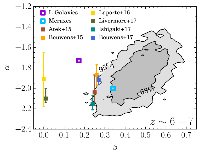
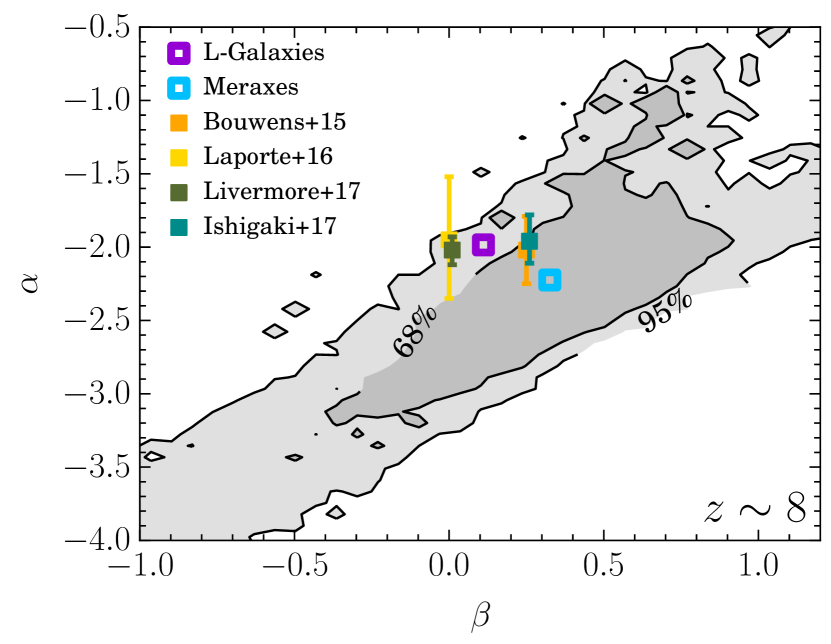
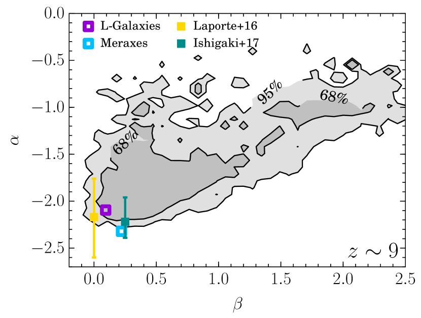
Figure 10.— Correlations between the faint-end slope of the luminosity function, $\alpha$, and the slope of the size–luminosity relation, $\beta$, overplotted with the observational results presented in Table 2 (filled squares) and simulation results (open squares). The top, middle, and bottom panels show the results at $z\sim 6-7$, $8$, and $9$, respectively.

We discuss here the intrinsic size–luminosity relation and UV luminosity function at $z\sim 6-7$, which are reliably estimated because of the large sample. The best-fit size–luminosity relation and its $1\sigma$ uncertainty are presented in the top panel of Figure 9, together with the results of previous work.

First, to evaluate the impact of detection incompleteness on the estimation of the size–luminosity relation, we fit the apparent size–luminosity distribution without correcting for completeness. In this process, as an alternative to $\Psi^{\prime}_{i}$ in Equation (16), we use a distribution model of

$$\Psi_{\mathrm{apparent}}(r_{\rm e},M_{\mathrm{UV}};r_{0},\sigma,\beta)$$

$$=P(r_{\rm e},M_{\mathrm{UV}};r_{0},\sigma,\beta),$$ (20)

where $P(r_{\rm e},M_{\mathrm{UV}})$ is described in Equation (13). This implies that we assume a flat distribution for the magnitude distribution. The best-fit parameter sets estimated using MLE are presented in Table 2 as “This work (apparent)”. We find that the modal sizes are $\sim 0.15$ dex underestimated, on average, and as large as $\sim 0.2$ dex at $M_{\mathrm{U}V}=-16$. The slope of the intrinsic size–luminosity relation is overestimated by $\Delta\beta=0.06$. This suggests that incompleteness has a slight contribution to the apparent steepness. In contrast, we find that the variance of the size–luminosity relation $\sigma$ is $\sim 25\%$ underestimated if incompleteness is not corrected for.

Then, we discuss the incompleteness-corrected results. Concerning the size–luminosity relation, the marginalized value of the slope is $\beta=0.46^{+0.08}_{-0.09}$. This slope is steeper than $\beta=0.25^{+0.25}_{-0.14}$ at $z\sim 5$ by Huang et al. (2013) (with incompleteness correction) and $\beta=0.25^{+0.05}_{-0.05}$ at $z\sim 6$ by Shibuya et al. (2015) (without incompleteness correction), both of them utilizing brighter ($M_{\mathrm{U}V}\lesssim-18$) samples. This is the first time to confirm the steepness of the intrinsic size–luminosity relation of $z\sim 6-7$ galaxies. Although a steep slope for galaxies at this redshift range was first reported by K15 based on reliable size measurements of the first HFF sample and then confirmed with larger samples by Bouwens et al. (2017a, c), none of these studies has applied incompleteness correction. The differences in the slope from Huang et al. (2013) and Shibuya et al. (2015) can be due to the differences in the magnitude range and hence in the physics dominating in galaxies. We further investigate this physical origin of the steepness in Section 5.3 using the result of the abundance matching by Behroozi et al. (2013). As described in the next paragraph, the difference from Shibuya et al. (2015) can also be explained by the differences in methods to measure magnitudes and to fit the size–luminosity relation. We note that although it has a steep slope, the best-fit intrinsic bivariate distribution predicts the existence of faint galaxies with large sizes, for instance, $M_{\mathrm{UV}}=-16$ galaxies with $r_{\mathrm{e}}\sim 1$ kpc, (see the top panel of Figure 5).

Shibuya et al. (2015) have found remarkably shallower slopes of $\beta\simeq 0.25\pm 0.05$ for brighter galaxies at $z\sim 6$ and $7$ even without correcting for incompleteness. Interestingly, in Figures 3 and 9, their galaxies appear to have a similar slope to ours. In fact, while their samples made public and plotted here use GALFIT magnitudes, they have used SExtractor magnitudes to derive the slope (T. Shibuya 2017, private communication). Applying the same method (Equation 20) to their sample, we find that using SExtractor magnitudes gives slopes $0.13$ and $0.21$ shallower than those based on GALFIT magnitudes at $z\sim 6$ and $7$, respectively. This may suggest that using SExtractor magnitudes leads them to derive the shallower slopes. In addition, our fitting method is different from theirs. They use a least-squares method that minimizes residuals only in size, which can bias the slope toward shallower values.

The modal size at $M_{\mathrm{U}V}=-21$ is $0.94^{+0.20}_{-0.15}\>\mathrm{kpc}$ at $z\sim 6-7$. This size can be slightly larger than the incompleteness-uncorrected sizes by the previous studies (Bouwens et al., 2004; Oesch et al., 2010a; Shibuya et al., 2015). We note that the sizes in Bouwens et al. (2004) and Oesch et al. (2010a) are averages in the range of $-21\leq M_{\mathrm{U}V}\leq-19.7$, which means the sizes at $M_{\mathrm{U}V}=-21$ should be larger (see also Figure 15).

The variance of the log-normal size distribution is $\sigma=0.87^{+0.10}_{-0.09}$. This is in good accordance with the values of $\sigma=0.83^{+0.046}_{-0.044}$ and $0.90^{+0.15}_{-0.065}$ at $z\sim 4$ and 5, respectively, in Huang et al. (2013). According to the analytical model by Mo et al. (1998) (see also Fall & Efstathiou, 1980), galaxy sizes are basically proportional to their halo sizes and spin parameters. The distribution of the spin parameter is log-normal at a fixed halo mass and thus also approximately log-normal at a fixed luminosity. Its variance was estimated to be $\sigma_{\mathrm{h}}=0.60$ at $z=0$ and revealed to scarcely evolve toward higher redshifts by Zjupa & Springel (2017) with the dark matter-only Illustris simulation. Since the observed variance of the galaxy-size distribution is larger than that of the spin parameter, there may be some elements that broaden the galaxy-size distribution. For example, a scatter in halo mass at fixed luminosity would result in a broader size distribution. This scatter was recently suggested at low redshifts in Charlton et al. (2017). Another explanation is a disk-to-halo ratio of specific angular momentum depending on the spin parameter, which means the galaxy size is no longer proportional to the spin parameter. We note that the derived variance $\sigma$ has been corrected for errors in size and magnitude measurements as described in Equation (17).

We find a shallow faint-end slope of the luminosity function of $\alpha=-1.86^{+0.17}_{-0.18}$, consistent with the slopes in Bouwens et al. (2015, 2017b) and Laporte et al. (2016) but slightly incompatible with recently suggested steep slopes of $\alpha\simeq-2.00$ to $-2.15$ (e.g., Livermore et al., 2017; Ishigaki et al., 2018). The reason for this is that our size–luminosity relation is steeper than those utilized in the previous studies. With a steeper size–luminosity relation, galaxies are easier to detect, and a smaller amount of incompleteness correction is needed in luminosity function derivation, especially at faint magnitude ranges. Thus, the faint-end slope becomes shallower. The effects of the size–luminosity relation on the luminosity function are further discussed in Section 5.4.

The characteristic magnitude, $M^{*}=-20.73^{+0.46}_{-0.81}$ is consistent with those of previous work. Since the marginalized distribution has a long tail toward the brighter magnitude, the mode of it is slightly larger, $M^{*}\simeq-20.56$. The uncertainty in $M^{*}$ is relatively large, probably because we do not use bright-galaxy samples from large-area surveys.

The parameters of the size–luminosity relation strongly correlate with those of the luminosity function. The most important may be the correlation between $\alpha$ and $\beta$, which has been pointed out by several works, including Grazian et al. (2011) and Bouwens et al. (2017a, b). The top panel of Figure 10 shows the correlation between $\alpha$ and $\beta$ obtained in this work together with the previous measurements of these parameters presented in Table 2. We find that the steeper $\alpha$ in Atek et al. (2015a) and Ishigaki et al. (2018) will become further consistent with ours if steeper size–luminosity relations are assumed. Even with our large and deep sample, at $z\sim 6-7$ there still remains a moderate uncertainty in $\alpha$ due to the uncertainty in the size–luminosity relation. This uncertainty in $\alpha$ is propagated to the UV luminosity density, a key quantity to calculating the number density of ionizing photons, although no previous studies on cosmic reionization have considered this uncertainty. We note that although the values of $\alpha$ obtained in Laporte et al. (2016) and Livermore et al. (2017) are consistent with our value, their $\alpha$–$\beta$ combinations are outside (with a large margin) of the 95% confidence ellipse obtained in this study. This demonstrates that these parameters must not be determined independently.

We also compare our $\alpha$ and $\beta$ measurements with the results of the semi-analytical model of galaxy formation L-Galaxies (Henriques et al., 2015). We run the L-Galaxies code on two $N$-body dark matter simulations of different resolutions, the Millennium (Springel et al., 2005) and Millennium-II (Boylan-Kolchin et al., 2009), and combine the two galaxy catalogs to probe a wide halo mass range. Applying Equation (12) to the combined catalog finds that the L-Galaxies predicts an $\alpha$ consistent with our value but a significantly flatter $\beta$. Results of the semi-analytical model of galaxy formation meraxes (Mutch et al., 2016; Liu et al., 2017) are also compared. We find a good agreement with our results for $z\sim 6-7$ and 8 and an acceptable agreement for $z\sim 9$. Note that the values of $\beta$ obtained here are different from those obtained in Liu et al. (2017) because of different fitting methods.

However, we find that the two models tend to predict relatively flatter size–luminosity relations, especially at $z\sim 6-7$ and 9. Their sizes are calculated essentially based on the analytical model by Mo et al. (1998). The flatter size–luminosity relations than observed may suggest the importance of careful calculations of the exchange of angular momentum between the dark matter halo and the stellar disk. Indeed, meraxes assumes a constant specific angular momentum of $j_{\mathrm{d}}/m_{\mathrm{d}}=1$, which disagrees with our result in Section 5.3. In L-Galaxies, specific angular momenta are calculated and compared with those by other semi-analytical models and hydrodynamical simulations (e.g. Guo et al., 2016; Hou et al., 2017). However, we do not discuss their results because they provide only the specific angular momenta of cooled gas, which may be systematically different from the specific angular momenta of disks, $j_{\mathrm{d}}/m_{\mathrm{d}}$. Further comparison between the observations and simulations is beyond the scope of this paper.

Another parameter set that shows a strong correlation is $\alpha$ and $M^{*}$, as seen in Figure 6 and as has been reported in previous studies. We confirm that the uncertainty in $\alpha$ decreases from $\sim 0.2$ to $\lesssim 0.1$ if $M^{*}$ is virtually fixed to, for instance, $M^{*}=-21$. The slope $\beta$ also correlates with the modal size $r_{0}$ and weakly with the width of the size distribution $\sigma$; both correlations originate from a requirement to reproduce small faint galaxies (except for the $\beta$–$\sigma$ correlation at $z\sim 9$).

Since $\alpha$ strongly correlates with $M^{*}$ and $\beta$, a more accurate measurement of $\alpha$ requires a larger sample containing bright objects (to better constrain $M^{*}$) accompanied by a completeness estimation on the size–luminosity plane (to obtain an unbiased $\beta$ value).

5.2. The Intrinsic Size–luminosity Relation
and Luminosity Function at $z\sim 8$ and 9

The fitting results of the intrinsic size–luminosity distributions at $z\sim 8$ and $9$ are presented in the middle and bottom panels of Figure 9, respectively. Since the samples are smaller than that at $z\sim 6-7$, the uncertainties in the parameters are typically $\gtrsim 2-3$ times larger.

Similar to that at $z\sim 6-7$, we find steep slopes of the size–luminosity relations of $\beta=0.38^{+0.28}_{-0.78}$ and $0.56^{+1.01}_{-0.27}$ at $z\sim 8$ and $9$, respectively. These are steeper than the slope of $\beta=0.19^{+0.25}_{-0.25}$ at $z\sim 8$ by Shibuya et al. (2015), although the differences are within the $1\sigma$ errors. However, the distributions of our galaxies on the size–luminosity plane appear to be consistent with theirs, as is the case for $z\sim 6-7$.

The modal sizes at $M_{\mathrm{U}V}=-21$ are $0.81^{+5.28}_{-0.26}\>\mathrm{kpc}$ and $1.20^{+367.64}_{-0.74}\>\mathrm{kpc}$ at $z\sim 8$ and 9, respectively. If incompleteness is not corrected for, the sizes become 0.2–0.3 dex smaller at $z\sim 8$ and 9, a slightly larger amount of decrease than that at $z\sim 6-7$. These are consistent with the incompleteness-uncorrected sizes of $r_{\mathrm{e}}=0.419^{+1.981}_{-0.262}$ at $z\sim 8$ by Shibuya et al. (2015) and $r_{\mathrm{e}}=0.6^{+0.3}_{-0.3}$ at $z\sim 9$ by Holwerda et al. (2015).

The variance of the size distribution $\sigma$ is $0.80^{+1.07}_{-0.26}$ and $1.04^{+1.52}_{-0.46}$ at $z\sim 8$ and 9, respectively, being almost constant at $z\sim 6-9$. While we do not find any indication of the evolution of $\sigma$ over this redshift range, the modal value of the variance distribution may decrease with redshift. Further discussion needs larger samples.

While the faint-end slope of the luminosity function at $z\sim 9$ is relatively shallow ($\alpha=-1.64^{+0.61}_{-0.28}$), that at $z\sim 8$ may be steep ($\alpha=-2.26^{+0.49}_{-0.99}$). However, both values are consistent with the value at $z\sim 6-7$ due to the large uncertainties.

At $z\sim 8-9$, the probability distributions of $M^{*}$ have tails toward the brighter magnitudes, and thus the median values are remarkably brighter than that at $z\sim 6-7$. This is because our samples do not have enough bright galaxies due to the small cosmic volume the HFF program is probing. We note that the $M^{*}$ values at $z\sim 8-9$ are close to typical magnitudes at these redshifts of $M^{*}\sim-21$ within the uncertainties. Furthermore, the modes are $M^{*}=-19.95$ at $z\sim 8$ and $-19.80$ at $z\sim 9$.

We also calculate $r_{0}$, $\sigma$, $\beta$, and $\alpha$ by fixing $M^{*}$ to $-20.73$, the best-fit value at $z\sim 6-7$, and obtain $(r_{0}/\mathrm{kpc},\sigma,\beta,\alpha)=(0.75^{+0.53}_{-0.16},0.65^{+0.35}_{-0.14},0.50^{+0.16}_{-0.21},-1.80^{+0.22}_{-0.30})$ at $z\sim 8$ and $(0.59^{+0.61}_{-0.16},0.69^{+0.40}_{-0.20},0.42^{+0.17}_{-0.15},-1.59^{+0.19}_{-0.18})$ at $z\sim 9$, as presented in Table 2. These $\alpha$ values are even shallower than those from the full modeling, with the uncertainties being reduced to be comparable to those of previous studies.

The middle and bottom panels of Figure 10 are the same as the top panel but for $z\sim 8$ and $9$, respectively. In contrast to the case for $z\sim 6-7$, all the $\alpha$–$\beta$ combinations from previous observations and L-Galaxies are within the 95% confidence contour of our results. Besides the parameter sets of $(\alpha,\beta)$, $(\alpha,M^{*})$, $(r_{0},\beta)$, and $(\sigma,\beta)$ that show correlations at $z\sim 6-7$, $r_{0}$ and $\sigma$ also correlate strongly at $z\sim 8-9$. This correlation is to reproduce the smaller galaxies and may indicate that we still do not trace the peak of the size distributions at $z\gtrsim 8$.

We find that the parameters of the size–luminosity relations and luminosity functions at $z\sim 8-9$ are still not well constrained. Thus, there are significant uncertainties in the luminosity function the faint-end slope of the luminosity function $\alpha$ and hence in discussions of reionization based on the UV luminosity density.

5.3. The Modeling of the Size–luminosity Relation

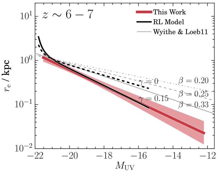
Figure 11.— Model predictions of the size–luminosity relation at $z\sim 6-7$, overplotted with the fitting result to the observation. The black solid and dashed lines show the predictions by the RL model with $\gamma=0.15$ and $0$, respectively. The gray dash-dotted, dashed, and solid lines represent the predictions by the Wyithe & Loeb (2011) model with $\beta=0.20$, $0.25$, and $0.33$, respectively, normalized to agree with those by the RL model at $M_{\mathrm{UV}}=-21$.

We construct a model to predict the normalization and slope of the size–luminosity relation at $z\sim 6-7$ in the following process, which is referred to as the RL model. (1) We calculate the average stellar mass of galaxies as a function of luminosity using the stellar mass–luminosity relation by González et al. (2011). (2) Combining step (1) with the stellar mass–halo mass relation by Behroozi et al. (2013), we evaluate the average halo mass of galaxies as a function of luminosity. Note that an extrapolated relation covering a wider mass range than that presented in their paper is utilized (P. Behroozi 2016, private communication). (3) We calculate the virial radius of halos by

$$r_{\mathrm{vir}}=\left[\frac{2GM_{\mathrm{vir}}}{\Delta_{\mathrm{vir}}{H(z)}^{2}}\right]^{1/3}.$$ (21)

In the calculation of the virial overdensity $\Delta_{\mathrm{vir}}$, we use the fitted form of $\Delta_{\mathrm{vir}}=18\pi^{2}+82x-39x^{2}$ with $x=\Omega_{\mathrm{m}}(z)-1$ by Bryan & Norman (1998). (4) From the halo radius, we calculate the galaxy size based on the equation in Mo et al. (1998),

$$r_{\mathrm{e}}=\frac{1.678}{\sqrt{2}}f_{j}\lambda f_{\mathrm{c}}^{-1/2}f_{\mathrm{R}}r_{\mathrm{vir}},$$ (22)

where $\lambda$ is the spin parameter of the halo defined in Peebles (1969). The factor $f_{j}(M_{\mathrm{vir}})$ represents the ratio of the specific angular momentum in the galaxy against that in the halo,

$$f_{j}(M_{\mathrm{vir}}) =\frac{j_{\mathrm{d}}}{m_{\mathrm{d}}}(M_{\mathrm{vir}})$$ (23)

$$=\left(\frac{j_{\mathrm{d}}}{m_{\mathrm{d}}}\right)_{M_{\mathrm{UV}}=-21}\left(\frac{M_{\mathrm{vir}}}{M_{\mathrm{vir,0}}}\right)^{\gamma},$$ (24)

where $j_{\mathrm{d}}$ and $m_{\mathrm{d}}$ are the ratio of the angular momentum and mass, respectively, in the galaxy against those in the halo. In contrast to the original equation in Mo et al. (1998), we allow $j_{\mathrm{d}}/m_{\mathrm{d}}$ to vary as a function of the halo mass, whose dependence was suggested in several observational studies (e.g., Somerville et al., 2017; Okamura et al., 2018) and simulations of galaxy formation (e.g., Sales et al., 2010). The factor $(j_{\mathrm{d}}/m_{\mathrm{d}})_{M_{\mathrm{UV}}=-21}$ and $M_{\mathrm{vir,0}}$ represent the $j_{\mathrm{d}}/m_{\mathrm{d}}$ and the halo mass of galaxies with $M_{\mathrm{UV}}=-21$, respectively. The index $\gamma$ is the exponent of the mass dependence of $j_{\mathrm{d}}/m_{\mathrm{d}}$. The factor $f_{j}$ equates to the original constant $j_{\mathrm{d}}/m_{\mathrm{d}}$ when $\gamma=0$. The factor $f_{\mathrm{c}}(c)$, depending only on the concentration parameter of the halo $c$, is to correct for the effect caused by the change in the density profile from the isothermal sphere to the NFW profile. The other factor $f_{\mathrm{R}}(j_{\mathrm{d}}/m_{\mathrm{d}},m_{\mathrm{d}},\lambda,c)$ is to correct for effects caused by the change in the density profile and the gravitational effect by the disk. We need the factor of $1.678$ to convert the scale length of the exponential profile to the half-light radius $r_{\mathrm{e}}$. Thus, we obtain the model of the size–luminosity relation.

Except for $\gamma$, there are four parameters that are needed to calculate the size; while $\lambda$ and $c$ are reliably determined in simulations (e.g., Bullock et al., 2001; Vitvitska et al., 2002; Davis & Natarajan, 2009; Prada et al., 2012), the parameters $j_{\mathrm{d}}$ and $m_{\mathrm{d}}$, depending on baryonic physics, are difficult to predict. In the calculation of the size, we assume $\lambda=0.04$ that is independent of redshift, which is consistent with the recent result in Zjupa & Springel (2017). For the concentration parameter $c$, we utilize the fitting function for the $c$–$M_{\mathrm{vir}}$ relation for Planck cosmology in Correa et al. (2015). We assume the typical values of $(j_{\mathrm{d}}/m_{\mathrm{d}})_{M_{\mathrm{UV}}=-21}=1.0$ (e.g., Fall & Efstathiou, 1980; Mo et al., 1998; Romanowsky & Fall, 2012; Fall & Romanowsky, 2013) and $m_{\mathrm{d}}=0.05$ (e.g., Sales et al., 2010). These values of $j_{\mathrm{d}}$ and $m_{\mathrm{d}}$ are shown to be consistent with observations in Section 5.5.

The calculated size–luminosity relation at $z\sim 6-7$ is presented in Figure 11 as the RL model. We find that the RL model predicts a shallow slope of $\beta\simeq 0.3$ when $\gamma=0$. While this shallow slope is consistent with observed slopes at lower redshifts of $\beta\sim 0.25$ (e.g., de Jong & Lacey, 2000; Huang et al., 2013; Shibuya et al., 2015, see also Figure 14), it is inconsistent with our steep slope at $z\sim 6-7$. However, when we change $f_{j}$ as a function of halo mass with $\gamma=0.15$, the model predicts a steeper slope that is consistent with the observed value at $z\sim 6-7$. This may suggests that $j_{\mathrm{d}}/m_{\mathrm{d}}$, that is, the fraction of the specific angular momentum in the galaxy, is smaller in fainter galaxies at higher redshifts. In the beginning stage of galaxy formation, stars are formed preferentially from gas with lower angular momenta. The halo mass dependence of $f_{j}$ obtained here may suggest that the faint galaxies are indeed in such a stage.

Stellar feedback may be another explanation because it redistributes the angular momentum between the galaxy and the halo, thus changing $f_{j}$. Genel et al. (2015) have used the Illustris cosmological simulation to find that stellar feedback increases the specific angular momentum of galaxies, although the halo mass dependence is equivalent to $\gamma<0$, opposite to what we find here (see also Sales et al. 2010 for a contradictory result).

Another possibility is that in low-mass halos, only those with relatively small spin parameters can form disks, thus making the slope steeper even with $\gamma=0$. If this is the case, the shape and variance of the log-normal size distribution at faint magnitudes can be different from those at bright magnitudes.

We also compare the obtained intrinsic slope with analytical predictions by Wyithe & Loeb (2011), which are shown in Figure 11 with gray lines. They construct a simple analytical model that describes the relation between the size and luminosity (see also Liu et al., 2017). The predicted relation depends on the feedback that dominates in galaxies. They test three kinds of feedback: energy conserving, momentum conserving, and no feedback. The predicted slopes are $\beta=0.20$, $0.25$, and $0.33$, respectively, all of which are shallower than the observed value at $>1\sigma$ levels. We note that they assume a constant $f_{j}$, which corresponds to $\gamma=0$.

Very recently, Ma et al. (2017) have suggested that UV light does not necessarily trace the main part of galaxies using high-resolution cosmological zoom-in simulations from the FIRE project. This observational bias might affect our discussion presented here and might lead to a smaller $\gamma$ (see also Huang et al., 2017; Somerville et al., 2017).

5.4. The Size–luminosity relations for Derivations of Luminosity Functions

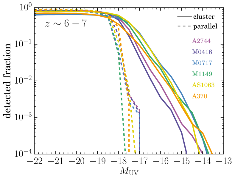
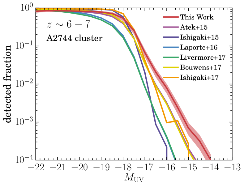
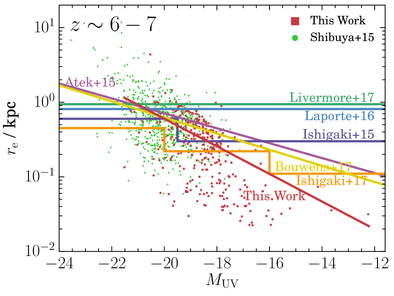
Figure 12.— (Top) Detected fraction against UV absolute magnitude in each field at $z\sim 6-7$ calculated using the completeness map of the field and the best-fit size–luminosity relation at $z\sim 6-7$. The solid and dashed lines correspond to the cluster and parallel fields, respectively. (Middle) Variation in the detected fractions at $z\sim 6-7$ in the Abell 2744 cluster field calculated with size–luminosity relations given in previous studies. The uncertainty estimated in this work is also plotted by the red shaded region. (Bottom) Size–luminosity relations in the previous studies utilized to calculate the detected fractions in the middle panel, overplotted with the galaxy distributions from this work (red points) and Shibuya et al. (2015) (green points).

In this subsection, we examine the effects of the size–luminosity relation on the estimation of the detected fraction of galaxies, and thus of the luminosity function.

The top panel of Figure 12 shows the detected fraction against UV magnitude for $z\sim 6-7$ calculated for all of the HFF cluster and parallel fields using the best-fit size–luminosity relation. As shown in this figure, the detected fraction at the faintest magnitudes $M_{\mathrm{U}V}\simeq-15$ to $-14$ is extremely low. This implies that the luminosity function is calculated from only a small part of galaxies in the field of view with a large ($\sim 10^{3}$) incompleteness correction.

We calculate the detected fractions, as an example, in the Abell 2744 cluster field assuming the six size–luminosity relations utilized in the previous studies at $z\sim 6-7$ (Atek et al., 2015a; Ishigaki et al., 2015, 2018; Laporte et al., 2016; Livermore et al., 2017; Bouwens et al., 2017b). These fractions, together with that calculated assuming our size–luminosity relation considering its uncertainty, are shown in the middle panel of Figure 12. The assumed size–luminosity relations are presented in the bottom panel of Figure 12. Whereas the relations in Ishigaki et al. (2015, 2018) have delta-function-like size distributions, those in Atek et al. (2015a), Laporte et al. (2016), Livermore et al. (2017), and Bouwens et al. (2017b) have variances of $\sigma\simeq 0.9$, 0.9, 1.0, and 0.69, respectively. As shown in the bottom panel, all of the size–luminosity relations in the previous studies are considerably flatter than ours, which results in underestimation of the detected fraction and a steeper faint-end slope of the luminosity function. Furthermore, there is a considerable difference between the relations, which introduces a significant uncertainty in the detected fraction and, consequently, in the luminosity function. In contrast, the uncertainty in the detected fraction calculated by our size–luminosity relation is smaller than the scatter of the detected fractions by the relations in the previous studies. This means that we reduce the uncertainty in the luminosity function that originates from the size–luminosity relation (the middle panel of Figure 12).

Our size–luminosity relations are more accurate than those in previous studies at $z\sim 6-9$ for three reasons: they are not extrapolations from low-redshift results but are determined directly from large samples with accurate size measurements, they are corrected for detection incompleteness, and proper statistics are utilized.

5.5. Redshift Evolution of Size

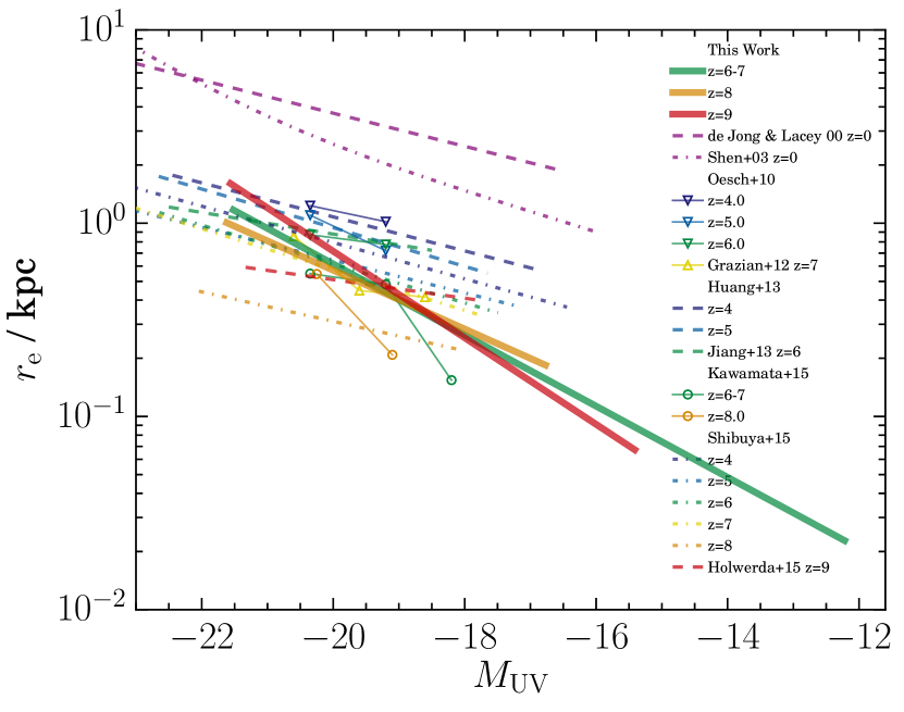
Figure 13.— Compilation of size–luminosity relations of LBGs from $z\sim 4$ to $z\sim 9-10$ (Huang et al. 2013, Jiang et al. 2013 [LAEs+LBGs], Oesch et al. 2010a, Grazian et al. 2012, Kawamata et al. 2015, Shibuya et al. 2015, and Holwerda et al. 2015) and spiral galaxies at $z=0$ (de Jong & Lacey 2000, Shen et al. 2003), with our results plotted by thick solid lines. Redshift is coded by color: purple, $z=0$; violet, $z\sim 4$; blue, $z\sim 5$; green, $z\sim 6$ ($z\sim 6-7$ for our result); yellow, $z\sim 7$; orange, $z\sim 8$; and red, $z\sim 9-10$ ($z\sim 9$ for our result). Different symbols represent the average absolute magnitudes and sizes of different samples: inverse triangles, $z\sim 4-6$ samples by Oesch et al. (2010a); triangles, $z\sim 7$ sample by Grazian et al. (2012); and circles, $z\sim 6-8$ samples by Kawamata et al. (2015). The purple dashed and dot-dashed lines represent the relations of $z\sim 0$ disk galaxies obtained by the measurements in the $i$ band by de Jong & Lacey (2000) and $r$ band by Shen et al. (2003), respectively. The violet, blue, and green dashed lines represent the fitting results to the sample of $z\sim 4$ and $5$ LBGs by Huang et al. (2013) and $z\sim 5.7-6.5$ Ly$\alpha$ emitters and LBGs by Jiang et al. (2013), respectively.

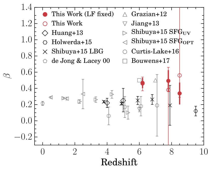
Figure 14.— Redshift evolution of the slope of the size–luminosity relation. The red circles show our measurements, while black symbols those of LBGs obtained by previous studies with two-dimensional profile fitting. The gray symbols represent results for non-LBG samples or those not based on two-dimensional profile fitting. The error bars correspond to the $1\sigma$ standard errors. The bold error bars of our samples show the $1\sigma$ standard errors where the parameters of the luminosity functions are fixed to the $z\sim 6-7$ best-fit values.

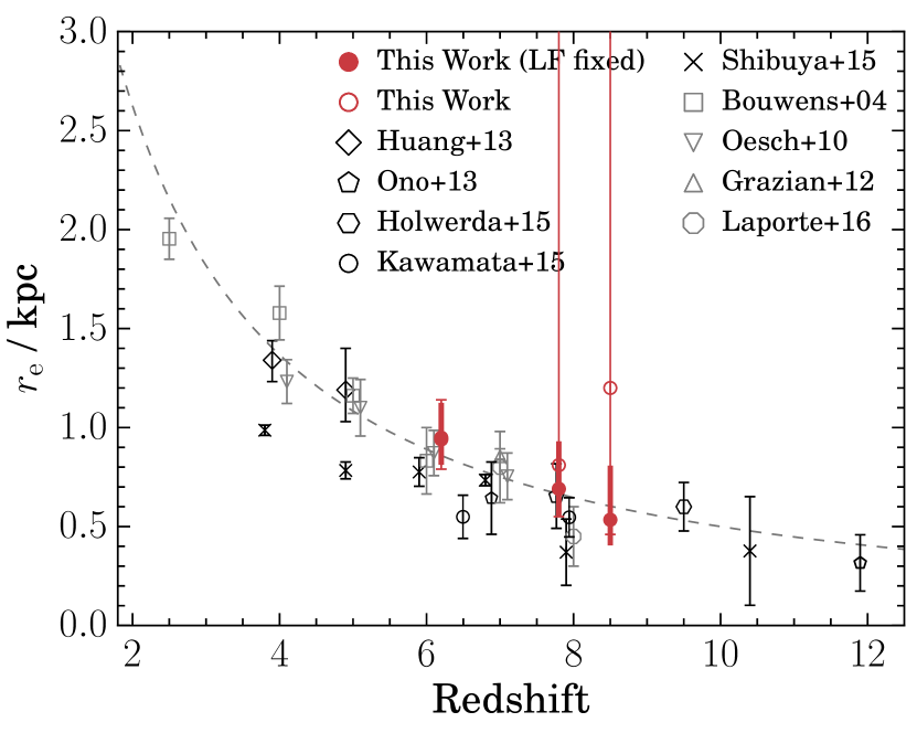
Figure 15.— Redshift evolution of the average size of bright galaxies at $-21\lesssim M_{\mathrm{UV}}\lesssim-19.7$. The red circles show our measurements, while the black symbols show those of LBGs obtained by previous studies. The gray dashed line represents the best-fit function of $r_{\mathrm{e}}\propto(1+z)^{-m}$ with $m=1.28$. The error bars correspond to the $1\sigma$ standard errors. The bold error bars of our samples show the $1\sigma$ standard errors where the parameters of the luminosity functions are fixed to the $z\sim 6-7$ best-fit values.

Table 3Luminosities Where the Average Sizes in Figure 15 Are Calculated

References	$\overline{M_{\mathrm{UV}}}$
This work	$-21$
Bouwens et al. (2004)	$-20.35$
Oesch et al. (2010a)	$-20.35$
Grazian et al. (2012)	$-20.50$
Huang et al. (2013)	$-21$
Ono et al. (2013) at $z\sim 7$	$-20.2$
Ono et al. (2013) at $z\sim 8$	$-20.15$
Kawamata et al. (2015) at $z\sim 6-7$	$-20.2$
Kawamata et al. (2015) at $z\sim 8$	$-20.30$
Holwerda et al. (2015)	$-20.87$
Shibuya et al. (2015)	$-21$
Laporte et al. (2016)	$-20.35$

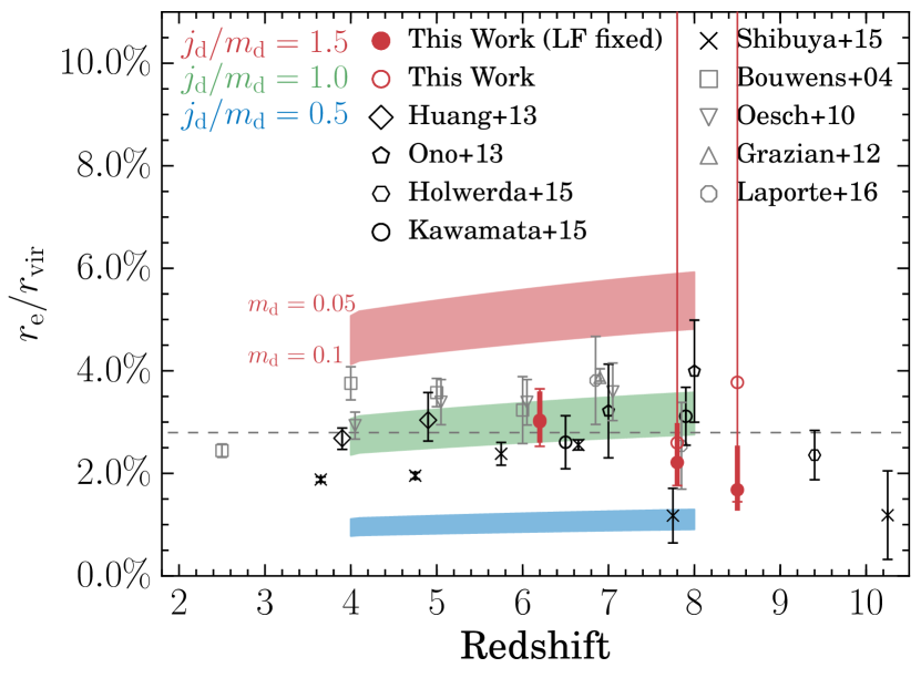
Figure 16.— Redshift evolution of the galaxy size–halo size ratio. Our samples are shown with red circles, and those from previous studies are in black. The errors in disk sizes only (plotted in Figure 15) are considered. The gray dashed line shows the average size ratio. The red, green, and blue shaded bands represent the ratio predicted by the model described in Section 5.5 with $\left({j_{\mathrm{d}}}/{m_{\mathrm{d}}}\right)_{M_{\mathrm{UV}}=-21}=1.5$, 1.0, and 0.5, respectively, where the width of each band indicates a weak dependence of the ratio on $m_{\mathrm{d}}$ and the upper and lower edges of each band correspond to $m_{\mathrm{d}}=0.05$ and 0.1, respectively.

Figure 13 shows the redshift evolution of the size–luminosity relation. While Oesch et al. (2010a), Grazian et al. (2012), Huang et al. (2013), Holwerda et al. (2015), Kawamata et al. (2015), and Shibuya et al. (2015) showed the relations of LBGs, Roche et al. (1996), de Jong & Lacey (2000), and Jiang et al. (2013) showed those of irregular galaxies, local spiral galaxies, and a combined sample of Ly$\alpha$ emitters (LAEs) and LBGs, respectively. The slopes at $z\sim 6-9$ are slightly steeper than those at $z\lesssim 5$ and those derived from bright samples at $z\gtrsim 6$. This may suggest that physical processes that affect the slopes, such as the formation stage, feedback, and transfers and redistributions of angular momentum, differ at around $z\sim 6$, especially for faint galaxies.

Figure 14 shows the redshift evolution of $\beta$ based on LBG samples by two-dimensional profile size measurements. While our fiducial values, where all uncertainties are considered, are plotted with red open circles and thin error bars, values where the parameters of the luminosity functions are fixed to the $z\sim 6-7$ best-fit values are plotted with red filled circles and bold error bars and presented in Table 2. For comparison, we also plot results from samples of non-LBGs and samples based on other size measurement methods. This figure shows that the slopes of our faint LBGs at $z\gtrsim 6$ are steeper than those of bright or lower-redshift galaxies, which are almost constant at $\beta\simeq 0.2$–0.3.

The redshift evolution of sizes at $-21\lesssim M_{\mathrm{U}V}\lesssim-19.7$ ($(0.3-1)L^{*}_{z=3}$) is presented in Figure 15, where $L^{*}_{z=3}$ is the characteristic UV luminosity of $z\sim 3$ LBGs obtained in Steidel et al. (1999). Similar to Figure 14, we plot our fiducial values and values where the parameters of the luminosity functions are fixed. Our samples give consistent results with previous measurements. We fit ${r_{\mathrm{e}}}\propto(1+z)^{-m}$ to data that are based on two-dimensional size measurements at $4<z<9.5$ (except for those by Shibuya et al. 2015, because they seem to be considerably smaller than the others). For our data, we use the ones where the parameters of the luminosity functions are fixed for consistency with the previous studies. We obtain $m=1.28\pm 0.11$, which is consistent within the errors with previous work (Bouwens et al., 2004; Oesch et al., 2010a; Ono et al., 2013; Kawamata et al., 2015; Holwerda et al., 2015; Shibuya et al., 2015). The index is predicted by analytical models to be $m=1.0$ for halos with a fixed mass and $m=1.5$ for halos with a fixed circular velocity (e.g., Ferguson et al., 2004). We find that we trace halos in the middle of the two states, as reported in previous work.

We note that the difference in the luminosity range makes the comparison between the samples difficult. The average luminosities of individual samples plotted in Figure 13 have some variance, as shown in Table 3. For instance, at $z=7$, a difference of 0.5 mag in luminosity corresponds to a difference in stellar mass of $\Delta M^{*}/M^{*}=54\%$, assuming the mass-luminosity relation in González et al. (2011). Based on the stellar mass–halo mass relation by Behroozi et al. (2013), the difference in stellar mass at $M_{\mathrm{UV}}=-21$ is equivalent to those in halo mass and halo radius of $\Delta M_{\mathrm{vir}}/M_{\mathrm{vir}}=52\%$ and $\Delta r_{\mathrm{vir}}/r_{\mathrm{vir}}=21\%$, respectively. Since the galaxy size is fundamentally proportional to the halo size, the expected galaxy size would differ $\Delta r_{\mathrm{e}}/r_{\mathrm{e}}=21\%$. This means that the difference between samples in the luminosity range introduces a systematic uncertainty into the discussion of the evolution of the average size, which is conventional in previous studies.

In order to resolve the above problem and further investigate the size evolution of galaxies, we calculate the evolution of the galaxy size–halo size ratio following K15 (see also Shibuya et al., 2015; Okamura et al., 2018). We calculate size ratios with a similar method to that for the model construction described in Section 5.3. In order to estimate the average halo size of each sample from its average luminosity, we make use of the stellar mass–luminosity relation in Reddy & Steidel (2009) at $z\sim 2.5$ and that in González et al. (2011) at $z\sim 4-9.5$, the stellar mass–halo mass relation (Behroozi et al., 2013), and Equation (21). Then, we obtain the size ratio by dividing the galaxy size by the halo size. The stellar mass–luminosity relation in González et al. (2011) is originally obtained at $z\sim 4-7$, but we also apply the relation at $z\sim 8-9.5$. In the above process, the variance in luminosity between the samples is corrected for because fainter samples are assigned smaller halo sizes. The result is shown in Figure 16. We confirm that the size ratio is roughly constant over the wide redshift range of $2.5\lesssim z\lesssim 7.0$, and the average ratio is $2.80\%\pm 0.10\%$ over this redshift range. This value is in good agreement with those obtained in previous studies (Kawamata et al., 2015; Shibuya et al., 2015; Huang et al., 2017; Okamura et al., 2018; Somerville et al., 2017).

It appears from Figure 15 that the average size continues to decrease with redshift at $z\gtrsim 7$. This trend, if true, predicts that the size ratio starts to decrease at $z\gtrsim 7$ because the denominator (halo mass and hence halo size of $M_{\mathrm{UV}}\simeq-21$ galaxies) increases with redshift at $z\gtrsim 7$ according to the stellar mass–halo mass relation by Behroozi et al. (2013). This prediction is consistent with our size ratio measurements at $z\sim 8$ and 9 within the errors. This decreasing trend in the size ratio was not observed in our previous work, K15, because K15 linearly extrapolated the stellar mass–halo mass relation at $M_{\mathrm{h}}\simeq 10^{11}M_{\odot}$, while in reality, it has a knee at $M_{\mathrm{h}}\simeq 10^{11.3}M_{\odot}$, thus resulting in underestimation of the halo masses.

We compare the observed size ratios with those predicted by the model constructed in Section 5.3 with $\gamma=0$,

$$\frac{r_{\mathrm{e}}}{r_{\mathrm{vir}}}=\frac{1.678}{\sqrt{2}}\left(\frac{j_{\mathrm{d}}}{m_{\mathrm{d}}}\right)_{M_{\mathrm{UV}}=-21}\lambda f_{\mathrm{c}}^{-1/2}f_{\mathrm{R}}.$$ (25)

Since $f_{\mathrm{R}}$ strongly depends on $j_{\mathrm{d}}/m_{\mathrm{d}}$ and weakly on $m_{\mathrm{d}}$, the only uncertain parameter to calculate the size ratio is $\left({j_{\mathrm{d}}}/{m_{\mathrm{d}}}\right)_{M_{\mathrm{UV}}=-21}$. Following K15, we change $\left({j_{\mathrm{d}}}/{m_{\mathrm{d}}}\right)_{M_{\mathrm{UV}}=-21}$ with the updated size measurements and simulation results of $\lambda$ and $c$. Model-predicted size ratios are presented in Figure 16. Since they weakly depend on $m_{\mathrm{d}}$, we show with bands the uncertainty due to $m_{\mathrm{d}}$ within the range of $0.05-0.1$. If we assume the typical value of 0.05 for $m_{\mathrm{d}}$ (e.g., Sales et al., 2010), we confirm that the observed size ratios are in good accordance with the model ratios premised on $j_{\mathrm{d}}\sim m_{\mathrm{d}}$ at $M_{\mathrm{UV}}=-21$. This is why we have assumed $\left({j_{\mathrm{d}}}/{m_{\mathrm{d}}}\right)_{M_{\mathrm{UV}}=-21}=1.0$ and $m_{\mathrm{d}}=0.05$, when modeling the size–luminosity relation in Section 5.3.

Using a mass-complete sample at $z\sim 1-7$ from the FourStar Galaxy Evolution Survey, Allen et al. (2017) have found a slower size evolution of $r_{\mathrm{e}}\propto(1+z)^{-0.97\pm 0.02}$. Since the size evolution of LBGs is faster, they have concluded that LBGs do not represent the entire galaxy population. Considering their results, it should be noted that this study also might not be tracing the entire galaxy population at $z\sim 6-9$.

6. Conclusion

We have measured the intrinsic sizes and magnitudes of 334, 61, and 37 faint dropout galaxies at $z\sim 6-7$, 8, and 9, respectively, from the complete HFF data, properly correcting for the lensing effects by fitting the lensed images with lensing-distorted Sérsic profiles. These represent the largest samples, especially at faint magnitudes of $M_{\mathrm{UV}}=-18$ to $-12$, where luminosity function measurements have been made possible only recently. Systematic and random errors in sizes and magnitudes have been carefully estimated using Monte Carlo simulations.

Although the HFF observations reach the faintest galaxies with the help of cluster lensing, our samples still suffer from the incompleteness that faint but large galaxies are not detected in observations. Since the degree of incompleteness strongly depends on the intrinsic size–luminosity relation, we have conducted simultaneous maximum-likelihood estimation of the luminosity function and size–luminosity relation from the observed distribution of galaxies on the size–luminosity plane and examined correlations between the luminosity function and size–luminosity relation.

We have also updated our mass models for Abell 2744 and MACS J0416.1$-$2403, as well as newly constructed models for Abell S1063 and Abell 370, all of which are publicly available through the STScI website. The following are the main results of this paper.

1. We have found that the slope of the intrinsic size–luminosity relation of faint galaxies at $z\sim 6-7$ is considerably steeper ($\beta\simeq 0.46$) than those ($\beta\simeq 0.22$–0.25) at $z\sim 4-5$ and those ($\beta\simeq 0.25$) assumed in previous studies of the luminosity function at $z\sim 6-7$. As a result of the steep size–luminosity relation, a shallow faint-end slope of the luminosity function of $\alpha=-1.86^{+0.17}_{-0.18}$ has been derived. The values of $\beta$ and $\alpha$ at $z\sim 8$ and 9 are consistent with those at $z\sim 6-7$ but have large errors due to small sample sizes. Thus, at $z\sim 8$ and 9, the UV luminosity density is still highly uncertain, which has to be taken into account in the discussion of cosmic reionization.

2. We have quantified the correlation between the parameters of the size–luminosity relation and luminosity function. Among the parameter pairs, we have found strong correlations between the faint-end slope of the luminosity function and the slope of the size–luminosity relation, ($\alpha$, $\beta$), and between the faint-end slope and the characteristic magnitude of the luminosity function, ($\alpha$, $M_{\star}$). Although the values of $\alpha$ in several previous studies are consistent with our measurements, some of the previous results have been found to be located outside our confidence region in the $\alpha$–$\beta$ plane.

3. We have constructed an analytical model to reproduce the steep slope of the size–luminosity relation at $z\sim 6-7$ utilizing the result of the abundance matching in Behroozi et al. (2013). We have found that the steepness is not reproduced when $j_{\mathrm{d}}/m_{\mathrm{d}}$ is constant within the magnitude range studied here. One possible explanation for the steepness is that a smaller fraction of the specific angular momentum is transferred to the disk from its halo at fainter magnitudes. Another possible explanation is that low-mass halos can host galaxies only when they have relatively small halo spin parameters.

4. The average size at ($0.3-1)L^{*}_{z=3}$ gradually decreases with redshift with $(1+z)^{-m}$, where $m=1.28\pm 0.11$ over a redshift range of $4\lesssim z\lesssim 9.5$. However, we have pointed out that this conventional discussion of the size evolution suffers from systematic biases due to a variance in average luminosity between the samples. In order to overcome this issue, we have calculated the disk-to-halo size ratio to find $j_{\mathrm{d}}/m_{\mathrm{d}}\sim 1$ at $M_{\mathrm{UV}}=-21$.

Appendix A Mass Models

Among the six HFF clusters, we use our version 3 mass models constructed in Kawamata et al. (2016) for MACS J0717.5+3745 and MACS J1149.6+2223; update the version 3 models for Abell 2744 and MACS J0416.1$-$2403, which are now referred to as version 4 models; and newly construct mass models for the last two clusters, Abell S1063 and Abell 370, also referred to as version 4. In this section, we describe the two updated and the two newly constructed models, whose modeling strategy is the same as that established in Kawamata et al. (2016). The lensing calculation is conducted using glafic (Oguri, 2010), which adopts a parametric modeling method. A summary of the mass modeling is presented in Table 4, including the numbers of multiple images and the reduced $\chi^{2}$. The best-fit parameters of the mass components are shown in Tables 5–8. Tables 9–12 show the position and redshift constraints of the multiple images for each cluster, which are utilized in the model constructions. The positions of the multiple images and the critical curves of the best-fit models are shown in Figure 17. The root mean squares of the distances between positions of observed and model-predicted multiple images on the image plane are presented in Table 4. The relatively small root mean squares for our models indicate that they well reproduce the observations despite strict constraints due to large numbers of multiple images and spectroscopic redshifts.

A.1. Updated model for Abell 2744

After the publication of Kawamata et al. (2016), a new mass model was published by Mahler et al. (2018) that exploits new multiple images and spectroscopic redshifts of multiple images revealed by MUSE observation. Considering the results of the MUSE observation, we update our model by incorporating and removing 25 and six positions of multiple images, respectively. Specifically, we incorporate multiple image systems 39, 40, 42, 47, 50, 61, 63, and 147 and remove IDs 2.3, 5.1, 5.4, and 8.3 and system 62. The positions of IDs 33.3 and 34.3 are corrected. In addition, we incorporate 20 MUSE spectroscopic redshifts that are considered to be reliable based on their qualities and consistency with our mass model. The spectroscopic redshift of system 1 is updated, and 19 redshifts are newly determined for systems 2, 5, 8, 10, 22, 24, 26, 30, 31, 33, 34, 39, 40, 41, 42, 47, 61, 63, and 147. We add a mass component representing a multipole perturbation in order to better fit the observations. While the image plane rms increases by $0\farcs 05$, the reduced $\chi^{2}$ slightly decreases by 0.01 compared to our version 3 model.

A.2. Updated model for MACS J0416.1$-$2403

After the publication of Kawamata et al. (2016), a new mass model was published by Caminha et al. (2017) that exploits new multiple images and spectroscopic redshifts of multiple images revealed by the MUSE observation. Considering the results of the MUSE observation, we update our model by incorporating 22 positions of multiple images. Specifically, we incorporate systems 26, 58, 67, 92, 94, 95, 96, and 97, among which system 97 is found for the first time in this work. The position of ID 91.3 is corrected. In addition, we incorporate 18 MUSE spectroscopic redshifts that are considered to be reliable based on their qualities and consistency with our mass model. The spectroscopic redshifts incorporated are for systems 26, 33, 25, 38, 44, 47, 48, 49, 51, 55, 58, 67, 86, 91, 92, 94, 95, and 96. The image plane rms increases by $0\farcs 06$, and the reduced $\chi^{2}$ increases by 0.30 compared to our version 3 model.

A.3. Newly constructed model for Abell S1063

In order to construct a mass model for Abell S1063, we use multiple images identified in Balestra et al. (2013), Monna et al. (2014), Richard et al. (2014), Johnson et al. (2014), Karman et al. (2015), Caminha et al. (2016a, b), Diego et al. (2016a), and Karman et al. (2017). Spectroscopic redshifts of multiple images were obtained in Balestra et al. (2013), Richard et al. (2014), Johnson et al. (2014), Karman et al. (2015), Caminha et al. (2016a), Karman et al. (2017), and the GLASS program (Schmidt et al., 2014b; Treu et al., 2015). In addition, we find three new counterimages and 13 new systems, which sums up to 35 new multiple images. As a result, we use 40 systems from the literature and 13 new systems; the total number of multiple images is 141. The positional uncertainty in the multiple images is assumed to be $\sigma_{x}=0\farcs 4$ for all of them.

A.4. Newly constructed model for Abell 370

In order to construct a mass model for Abell 370, we use multiple images identified in Richard et al. (2010), Richard et al. (2014), Johnson et al. (2014), Diego et al. (2016b), and Lagattuta et al. (2017). Spectroscopic redshifts of multiple images were obtained in Richard et al. (2010, 2014), Lagattuta et al. (2017), and the GLASS program (Schmidt et al., 2014b; Treu et al., 2015). We correct the positions of four multiple images of IDs 3.3, 8.3, 13.3, and 26.3. In addition, we find two new counterimages and 16 new systems, which sums up to 40 new multiple images. As a result, we use 33 systems from the literature and 16 new systems; the total number of multiple images is 135. The positional uncertainty in the multiple images is assumed to be $\sigma_{x}=0\farcs 4$ for all of them.

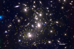
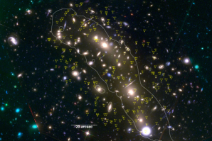
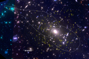
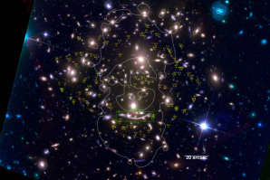
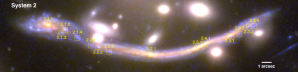
Figure 17.— Multiple image systems used for mass modeling for Abell 2744 (upper left), MACS J0416.1$-$2403 (upper right), Abell S1063 (middle left), and Abell 370 (middle right). The bottom panel shows zoomed-in images of System 2 in the Abell 370 field. Underlying color-composite images are created from the HST $B_{435}$+$V_{606}$-, $i_{814}$+$Y_{105}$-, and $J_{125}$+$J\!H_{140}$+$H_{160}$-band images. Small yellow squares show the positions of multiple images (see Tables 9–12 for details). Critical curves for a source redshift of $z=8$ are shown with white solid lines.

Table 4Summary of Version 4 Mass Modeling for Four Clusters

Cluster	No. of Multiple Image	No. of Multiple Images	$\chi^{2}$/dof	Image Plane rms
	Systems (with spec-$z$)			(arcsec)
Abell 2744	$45\ (24)$	$132$	130.2/134	0.42
MACS J0416.1$-$2403	$75\ (34)$	$202$	240.0/196	0.50
Abell S1063	$53\ (19)$	$141$	136.2/138	0.38
Abell 370	$49\ (19)$	$135$	99.5/140	0.50

Table 5Mass Model Parameters for Abell 2744

Component	Model	Mass	$e$	$\theta_{e}$	$c$	$\Delta x$	$\Delta y$
		$(10^{14}\ h^{-1}M_{\odot})$		(deg)		(arcsec)	(arcsec)
Cluster halo 1	NFW	$4.53^{+0.88}_{-0.80}$	$0.37^{+0.03}_{-0.03}$	$165.05^{+4.04}_{-2.88}$	$4.04^{+0.36}_{-0.33}$	$-0.21^{+0.41}_{-0.37}$	$3.30^{+0.53}_{-0.52}$
Cluster halo 2	NFW	$1.41^{+0.21}_{-0.22}$	$0.38^{+0.02}_{-0.02}$	$129.42^{+1.79}_{-2.02}$	$9.49^{+0.88}_{-0.69}$	$-18.69^{+0.18}_{-0.18}$	$-17.91^{+0.16}_{-0.17}$
Cluster halo 3	NFW	$0.21^{+0.07}_{-0.08}$	$0.76^{+0.03}_{-0.08}$	$107.61^{+9.78}_{-3.94}$	[$10.00$]	[$-26.97$]	[$30.91$]
		$\sigma_{*}\tablenotemark{b}$	$r_{\rm trun,*}$	$\eta$
		$({\rm km\ s^{-1}})$	(arcsec)
Member galaxies	GALS	$190.76^{+9.69}_{-9.94}$	$71.98^{+31.40}_{-19.06}$	$1.42^{+0.06}_{-0.11}$
		$z_{s,{\rm fid}}$	$\gamma\times 10^{2}$	$\theta_{\gamma}$
				(deg)
External perturbation	PERT	[$2.00$]	$8.97^{+0.85}_{-0.88}$	$139.31^{+2.05}_{-2.24}$
		$z_{s,{\rm fid}}$	$\epsilon\times 10^{2}$	$\theta_{\rm\epsilon}$	$m$	$n$
				(deg)
Multipole perturbation 1	MPOLE	[$2.00$]	$0.22^{+0.19}_{-0.11}$	$52.37^{+17.80}_{-12.16}$	[$3.00$]	[$2.00$]
Multipole perturbation 2	MPOLE	[$2.00$]	$1.22^{+0.26}_{-0.21}$	$93.97^{+1.96}_{-2.24}$	[$4.00$]	[$2.00$]

Note. — Numbers in square brackets are fixed during the model optimization.

Table 6Mass Model Parameters for MACS J0416.1$-$2403

Component	Model	Mass	$e$	$\theta_{e}$	$c$	$\Delta x$	$\Delta y$
		$(10^{14}\ h^{-1}M_{\odot})$		(deg)		(arcsec)	(arcsec)
Cluster halo 1	NFW	$2.78^{+0.37}_{-0.29}$	$0.66^{+0.01}_{-0.01}$	$60.58^{+0.65}_{-1.07}$	$4.18^{+0.33}_{-0.26}$	$-1.98^{+0.65}_{-0.49}$	$1.69^{+0.29}_{-0.37}$
Cluster halo 2	NFW	$2.23^{+0.71}_{-0.58}$	$0.69^{+0.02}_{-0.02}$	$42.93^{+0.97}_{-1.10}$	$4.45^{+0.77}_{-0.42}$	$21.95^{+0.58}_{-0.48}$	$-34.32^{+0.39}_{-0.41}$
Cluster halo 3	NFW	$1.18^{+0.52}_{-0.31}$	$0.61^{+0.04}_{-0.04}$	$37.66^{+2.24}_{-1.61}$	$4.19^{+0.63}_{-0.55}$	$24.40^{+0.57}_{-0.56}$	$-53.79^{+0.85}_{-0.95}$
		$\sigma_{*}\tablenotemark{b}$	$r_{\rm trun,*}$	$\eta$
		$({\rm km\ s^{-1}})$	(arcsec)
Member galaxies	GALS	$291.59^{+19.70}_{-16.41}$	$16.39^{+4.89}_{-3.13}$	$1.40^{+0.06}_{-0.10}$
		$\sigma$	$e$	$\theta_{e}$	$r_{\rm trun}$	$\Delta x$	$\Delta y$
		$({\rm km\ s^{-1}})$		(deg)	(arcsec)	(arcsec)	(arcsec)
Member galaxy	PJE	$118.69^{+46.15}_{-13.90}$	[$0.27$]	[$166.70$]	$1.81^{+3.48}_{-1.27}$	[$-14.56$]	[$15.28$]
		$z_{s,{\rm fid}}$	$\gamma\times 10^{2}$	$\theta_{\gamma}$
				(deg)
External perturbation	PERT	[$2.00$]	$3.49^{+0.95}_{-1.02}$	$27.89^{+4.62}_{-6.26}$
		$z_{s,{\rm fid}}$	$\epsilon\times 10^{2}$	$\theta_{\rm\epsilon}$	$m$	$n$
				(deg)
Multipole perturbation	MPOLE	[$2.00$]	$1.10^{+0.25}_{-0.22}$	$57.36^{+4.31}_{-3.56}$	[$3.00$]	[$2.00$]

Note. — Numbers in square brackets are fixed during the model optimization.

Table 7Mass Model Parameters for Abell S1063

Component	Model	Mass	$e$	$\theta_{e}$	$c$	$\Delta x$	$\Delta y$
		$(10^{14}\ h^{-1}M_{\odot})$		(deg)		(arcsec)	(arcsec)
Cluster halo 1	NFW	$11.47^{+0.99}_{-1.05}$	$0.46^{+0.01}_{-0.01}$	$53.38^{+0.33}_{-0.35}$	$5.15^{+0.25}_{-0.19}$	$-0.53^{+0.16}_{-0.15}$	$0.27^{+0.20}_{-0.17}$
Cluster halo 2	NFW	$0.47^{+0.14}_{-0.16}$	$0.77^{+0.02}_{-0.06}$	$70.84^{+2.30}_{-2.03}$	$2.92^{+1.57}_{-0.61}$	[$-84.67$]	[$45.07$]
Cluster halo 3	NFW	$0.04^{+0.02}_{-0.01}$	$0.62^{+0.06}_{-0.11}$	$102.80^{+5.63}_{-5.38}$	$7.94^{+2.48}_{-2.11}$	$16.02^{+1.23}_{-0.89}$	$-17.23^{+0.66}_{-0.54}$
		$\sigma_{*}\tablenotemark{b}$	$r_{\rm trun,*}$	$\eta$
		$({\rm km\ s^{-1}})$	(arcsec)
Member galaxies	GALS	$130.39^{+8.45}_{-7.39}$	$173.91^{+186.37}_{-72.16}$	$0.57^{+0.51}_{-0.22}$
		$z_{s,{\rm fid}}$	$\gamma\times 10^{2}$	$\theta_{\gamma}$
				(deg)
External perturbation	PERT	[$2.00$]	$3.93^{+0.72}_{-0.69}$	$37.58^{+3.16}_{-4.20}$

Note. — Numbers in square brackets are fixed during the model optimization.

Table 8Mass Model Parameters for Abell 370

Component	Model	Mass	$e$	$\theta_{e}$	$c$	$\Delta x$	$\Delta y$
		$(10^{14}\ h^{-1}M_{\odot})$		(deg)		(arcsec)	(arcsec)
Cluster halo 1	NFW	$0.70^{+0.22}_{-0.18}$	$0.50^{+0.06}_{-0.06}$	$5.80^{+4.00}_{-3.40}$	$10.05^{+3.42}_{-2.00}$	$3.69^{+0.69}_{-0.66}$	$-5.24^{+1.42}_{-1.93}$
Cluster halo 2	NFW	$16.57^{+6.82}_{-6.27}$	$0.28^{+0.06}_{-0.07}$	$154.22^{+11.20}_{-21.52}$	$1.62^{+0.31}_{-0.28}$	$-17.10^{+2.97}_{-3.63}$	$-4.55^{+2.37}_{-2.13}$
Cluster halo 3	NFW	$0.40^{+0.82}_{-0.27}$	$0.43^{+0.19}_{-0.32}$	$15.44^{+9.03}_{-6.18}$	$6.85^{+3.50}_{-1.84}$	$-6.55^{+0.82}_{-0.82}$	$-24.14^{+1.14}_{-1.11}$
Cluster halo 4	NFW	$1.52^{+0.67}_{-0.43}$	$0.15^{+0.05}_{-0.05}$	$164.13^{+15.39}_{-38.20}$	$8.80^{+2.11}_{-1.60}$	[$-5.88$]	[$-37.21$]
		$\sigma_{*}\tablenotemark{b}$	$r_{\rm trun,*}$	$\eta$
		$({\rm km\ s^{-1}})$	(arcsec)
Member galaxies	GALS	$235.92^{+35.58}_{-26.20}$	$23.60^{+17.36}_{-9.86}$	$1.41^{+0.07}_{-0.15}$
		$z_{s,{\rm fid}}$	$\gamma\times 10^{2}$	$\theta_{\gamma}$
				(deg)
External perturbation	PERT	[$2.00$]	$6.55^{+2.25}_{-2.35}$	$177.71^{+4.13}_{-5.64}$
		$z_{s,{\rm fid}}$	$\epsilon\times 10^{2}$	$\theta_{\rm\epsilon}$	$m$	$n$
				(deg)
Multipole perturbation 1	MPOLE	[$2.00$]	$1.69^{+0.29}_{-0.30}$	$43.57^{+3.32}_{-2.85}$	[$3.00$]	[$2.00$]
Multipole perturbation 2	MPOLE	[$2.00$]	$0.85^{+0.17}_{-0.19}$	$12.21^{+3.84}_{-3.00}$	[$4.00$]	[$2.00$]

Note. — Numbers in square brackets are fixed during the model optimization.

Table 9Abell 2744 Multiple Image Systems

ID	R.A.	decl.	$z_{\rm spec}$	$z_{\rm model}$	Photo-$z$ Prior	References
1.1	$3.597542$	$-30.403917$	1.688	$\cdots$	$\cdots$	JM, GM
1.2	$3.595958$	$-30.406822$		$\cdots$	$\cdots$	JM
1.3	$3.586208$	$-30.409986$		$\cdots$	$\cdots$	JM
2.1	$3.583250$	$-30.403350$	1.888	$\cdots$	$\cdots$	JM, GM
2.2	$3.597292$	$-30.396725$		$\cdots$	$\cdots$	JM
2.4	$3.586417$	$-30.402128$		$\cdots$	$\cdots$	JM
3.1	$3.589480$	$-30.393867$	3.980	$\cdots$	$\cdots$	JM, TJ
3.2	$3.588647$	$-30.393788$		$\cdots$	$\cdots$	JM
4.1	$3.592125$	$-30.402633$	3.580	$\cdots$	$\cdots$	JM, JR
4.2	$3.595625$	$-30.401622$		$\cdots$	$\cdots$	JM
4.3	$3.580417$	$-30.408925$		$\cdots$	$\cdots$	JM
4.4	$3.593208$	$-30.404914$		$\cdots$	$\cdots$	JR
4.5	$3.593583$	$-30.405106$		$\cdots$	$\cdots$	JR
5.2	$3.584982$	$-30.391374$	4.022	$\cdots$	$\cdots$	JM, GM
5.3	$3.579959$	$-30.394772$		$\cdots$	$\cdots$	JM
6.1	$3.598535$	$-30.401797$	2.019	$\cdots$	$\cdots$	JM, JR
6.2	$3.594042$	$-30.408011$		$\cdots$	$\cdots$	JM
6.3	$3.586417$	$-30.409372$		$\cdots$	$\cdots$	JM
7.1	$3.598261$	$-30.402322$	$\cdots$	$2.65^{+0.13}_{-0.12}$	$3.25\pm 0.5$	JM
7.2	$3.595233$	$-30.407407$	$\cdots$			JM
7.3	$3.584601$	$-30.409818$	$\cdots$			JM
8.1	$3.589708$	$-30.394339$	3.975	$\cdots$	$\cdots$	JM
8.2	$3.588834$	$-30.394222$		$\cdots$	$\cdots$	JM, GM
9.1	$3.588375$	$-30.405272$	$\cdots$	$2.46^{+0.36}_{-0.30}$	$\cdots$	JM
9.2	$3.587125$	$-30.406242$	$\cdots$		$\cdots$	JM
10.1	$3.588417$	$-30.405878$	2.656	$\cdots$	$\cdots$	JM, GM
10.2	$3.587375$	$-30.406481$		$\cdots$	$\cdots$	JM
11.1	$3.591375$	$-30.403858$	$\cdots$	$2.57^{+0.12}_{-0.11}$	$\cdots$	JM
11.2	$3.597264$	$-30.401431$	$\cdots$		$\cdots$	JM
11.3	$3.582792$	$-30.408914$	$\cdots$		$\cdots$	JM
11.4	$3.594542$	$-30.406542$	$\cdots$		$\cdots$	JR
12.2	$3.593239$	$-30.403249$	$\cdots$	$3.12^{+0.46}_{-0.42}$	$2.80\pm 0.5$	JR
12.3	$3.594555$	$-30.402996$	$\cdots$			JR
13.1	$3.592375$	$-30.402558$	$\cdots$	$1.41^{+0.04}_{-0.04}$	$\cdots$	JR
13.2	$3.593792$	$-30.402164$	$\cdots$		$\cdots$	JR
13.3	$3.582792$	$-30.408044$	$\cdots$		$\cdots$	JR
14.1	$3.589750$	$-30.394636$	$\cdots$	$2.58^{+0.12}_{-0.12}$	$\cdots$	JR
14.2	$3.588458$	$-30.394436$	$\cdots$		$\cdots$	JR
14.3	$3.577577$	$-30.401682$	$\cdots$		$\cdots$	MJ
18.1	$3.590750$	$-30.395561$	5.660	$\cdots$	$\cdots$	JR, XW
18.2	$3.588375$	$-30.395636$		$\cdots$	$\cdots$	JR
18.3	$3.576123$	$-30.404489$		$\cdots$	$\cdots$	DL
20.1	$3.596234$	$-30.402976$	$\cdots$	$2.55^{+0.12}_{-0.11}$	$\cdots$	DL
20.2	$3.595172$	$-30.405442$	$\cdots$		$\cdots$	DL
20.3	$3.581992$	$-30.409550$	$\cdots$		$\cdots$	MJ
21.1	$3.596176$	$-30.403117$	$\cdots$	$2.55^{+0.12}_{-0.11}$	$\cdots$	DL
21.2	$3.595259$	$-30.405342$	$\cdots$		$\cdots$	DL
21.3	$3.581973$	$-30.409600$	$\cdots$		$\cdots$	MJ
22.1	$3.587919$	$-30.411613$	5.284	$\cdots$	$\cdots$	DL, GM
22.2	$3.600059$	$-30.404395$		$\cdots$	$\cdots$	HA14
22.3	$3.596572$	$-30.409000$		$\cdots$	$\cdots$	HA14
23.1	$3.588157$	$-30.410550$	$\cdots$	$4.53^{+0.38}_{-0.32}$	$\cdots$	DL
23.2	$3.593552$	$-30.409709$	$\cdots$		$\cdots$	HA14
23.3	$3.600541$	$-30.401816$	$\cdots$		$\cdots$	HA14
24.1	$3.595902$	$-30.404467$	1.043	$\cdots$	$\cdots$	MJ, GM
24.2	$3.595114$	$-30.405909$		$\cdots$	$\cdots$	MJ
24.3	$3.587332$	$-30.409095$		$\cdots$	$\cdots$	MJ
25.1	$3.594476$	$-30.402742$	$\cdots$	$1.22^{+0.03}_{-0.03}$	$\cdots$	MJ
25.2	$3.592147$	$-30.403317$	$\cdots$		$\cdots$	MJ
25.3	$3.584215$	$-30.408284$	$\cdots$		$\cdots$	MJ
26.1	$3.593906$	$-30.409726$	3.054	$\cdots$	$\cdots$	DL, GM
26.2	$3.590350$	$-30.410584$		$\cdots$	$\cdots$	DL
26.3	$3.600099$	$-30.402976$		$\cdots$	$\cdots$	DL
28.1	$3.580452$	$-30.405043$	$\cdots$	$6.67^{+0.43}_{-0.42}$	$6.70\pm 0.5$	HA14
28.2	$3.597831$	$-30.395958$	$\cdots$			HA14
28.3	$3.585321$	$-30.397958$	$\cdots$			HA14
28.4	$3.587442$	$-30.401376$	$\cdots$			DL
29.1	$3.582437$	$-30.397575$	$\cdots$	$3.31^{+0.43}_{-0.38}$	$\cdots$	MJ
29.2	$3.580524$	$-30.400475$	$\cdots$		$\cdots$	MJ
30.1	$3.591016$	$-30.397439$	1.025	$\cdots$	$\cdots$	MJ, GM
30.2	$3.586669$	$-30.398184$		$\cdots$	$\cdots$	MJ
30.3	$3.581923$	$-30.401704$		$\cdots$	$\cdots$	MJ
31.1	$3.585925$	$-30.403159$	4.760	$\cdots$	$\cdots$	DL, GM
31.2	$3.583703$	$-30.404100$		$\cdots$	$\cdots$	DL
32.1	$3.583605$	$-30.404712$	$\cdots$	$4.46^{+0.40}_{-0.32}$	$\cdots$	MJ
32.2	$3.586667$	$-30.403337$	$\cdots$		$\cdots$	MJ
32.3	$3.599789$	$-30.395980$	$\cdots$		$\cdots$	MJ
33.1	$3.584708$	$-30.403152$	5.726	$\cdots$	$\cdots$	HA14, GM
33.2	$3.584396$	$-30.403400$		$\cdots$	$\cdots$	HA14
33.3	$3.600418$	$-30.395110$		$\cdots$	$\cdots$	GM
34.1	$3.593427$	$-30.410847$	3.785	$\cdots$	$\cdots$	MJ, GM
34.2	$3.593813$	$-30.410723$		$\cdots$	$\cdots$	MJ
34.3	$3.600711$	$-30.404604$		$\cdots$	$\cdots$	MJ
39.1	$3.588792$	$-30.392530$	4.015	$\cdots$	$\cdots$	MJ, GM
39.2	$3.588542$	$-30.392508$		$\cdots$	$\cdots$	MJ
39.3	$3.577479$	$-30.399568$		$\cdots$	$\cdots$	JM
40.1	$3.589086$	$-30.392668$	4.000	$\cdots$	$\cdots$	MJ, GM
40.2	$3.588193$	$-30.392551$		$\cdots$	$\cdots$	MJ
40.3	$3.577544$	$-30.399376$		$\cdots$	$\cdots$	JM
41.1	$3.599176$	$-30.399582$	4.911	$\cdots$	$\cdots$	MJ, GM
41.2	$3.593558$	$-30.407769$		$\cdots$	$\cdots$	MJ
41.3	$3.583446$	$-30.408500$		$\cdots$	$\cdots$	MJ
41.4	$3.590617$	$-30.404459$		$\cdots$	$\cdots$	GM
42.1	$3.597306$	$-30.400612$	3.692	$\cdots$	$\cdots$	MJ, GM
42.2	$3.590961$	$-30.403255$		$\cdots$	$\cdots$	MJ
42.3	$3.581584$	$-30.408635$		$\cdots$	$\cdots$	MJ
42.4	$3.594229$	$-30.406390$		$\cdots$	$\cdots$	MJ
42.5	$3.592413$	$-30.405194$		$\cdots$	$\cdots$	GM
46.1	$3.595007$	$-30.400759$	$\cdots$	$9.52^{+0.45}_{-0.41}$	$9.50\pm 0.5$	AZ
46.2	$3.592505$	$-30.401500$	$\cdots$			AZ
46.3	$3.577519$	$-30.408700$	$\cdots$			AZ
47.1	$3.590162$	$-30.392181$	4.022	$\cdots$	$\cdots$	GM, GM
47.2	$3.585842$	$-30.392244$		$\cdots$	$\cdots$	MJ
47.3	$3.578329$	$-30.398133$		$\cdots$	$\cdots$	MJ
50.1	$3.577973$	$-30.401600$	$\cdots$	$5.65^{+0.53}_{-0.47}$	$\cdots$	MJ
50.2	$3.593956$	$-30.394287$	$\cdots$		$\cdots$	MJ
53.1	$3.579838$	$-30.401592$	$\cdots$	$5.54^{+0.82}_{-0.72}$	$\cdots$	DL
53.2	$3.583548$	$-30.396700$	$\cdots$		$\cdots$	DL
54.1	$3.592350$	$-30.409892$	$\cdots$	$5.98^{+0.70}_{-0.55}$	$\cdots$	DL
54.2	$3.588254$	$-30.410325$	$\cdots$		$\cdots$	DL
54.5	$3.600920$	$-30.400825$	$\cdots$		$\cdots$	DL
55.1	$3.597042$	$-30.404753$	$\cdots$	$1.70^{+0.05}_{-0.05}$	$\cdots$	DL
55.2	$3.596417$	$-30.406125$	$\cdots$		$\cdots$	DL
55.3	$3.585744$	$-30.410100$	$\cdots$		$\cdots$	DL
56.1	$3.582542$	$-30.402272$	$\cdots$	$1.97^{+0.07}_{-0.07}$	$\cdots$	DL
56.2	$3.586250$	$-30.400850$	$\cdots$		$\cdots$	DL
56.3	$3.584500$	$-30.399286$	$\cdots$		$\cdots$	DL
56.4	$3.596750$	$-30.396300$	$\cdots$		$\cdots$	DL
59.1	$3.584284$	$-30.408925$	$\cdots$	$2.49^{+0.13}_{-0.12}$	$\cdots$	MI
59.2	$3.598125$	$-30.400981$	$\cdots$		$\cdots$	MI
60.1	$3.598075$	$-30.403989$	$\cdots$	$1.71^{+0.06}_{-0.06}$	$1.70\pm 0.5$	DL
60.2	$3.595729$	$-30.407558$	$\cdots$			DL
60.3	$3.587384$	$-30.410158$	$\cdots$			DL
61.1	$3.595533$	$-30.403499$	2.951	$\cdots$	$\cdots$	GM, GM
61.2	$3.595143$	$-30.404495$		$\cdots$	$\cdots$	MJ
63.1	$3.582261$	$-30.407166$	5.662	$\cdots$	$\cdots$	GM, GM
63.2	$3.592758$	$-30.407022$		$\cdots$	$\cdots$	GM
63.3	$3.589134$	$-30.403419$		$\cdots$	$\cdots$	GM
63.4	$3.598805$	$-30.398279$		$\cdots$	$\cdots$	XW
147.1	$3.589679$	$-30.392136$	4.022	$\cdots$	$\cdots$	MJ, GM
147.2	$3.586454$	$-30.392128$		$\cdots$	$\cdots$	MJ
147.3	$3.578009$	$-30.398392$		$\cdots$	$\cdots$	GM

Table 10MACS J0416.1$-$2403 Multiple Image Systems

ID	R.A.	decl.	$z_{\rm spec}$	$z_{\rm model}$	Photo-$z$ Prior	References
1.1	$64.040797$	$-24.061616$	1.896	$\cdots$	$\cdots$	AZ, LC
1.2	$64.043472$	$-24.063514$		$\cdots$	$\cdots$	AZ
1.3	$64.047367$	$-24.068673$		$\cdots$	$\cdots$	AZ
2.1	$64.041168$	$-24.061851$	1.893	$\cdots$	$\cdots$	AZ, CG
2.2	$64.043021$	$-24.063010$		$\cdots$	$\cdots$	AZ
2.3	$64.047484$	$-24.068851$		$\cdots$	$\cdots$	AZ
3.1	$64.030772$	$-24.067118$	1.989	$\cdots$	$\cdots$	AZ, CG
3.2	$64.035254$	$-24.070993$		$\cdots$	$\cdots$	AZ
3.3	$64.041797$	$-24.075743$		$\cdots$	$\cdots$	AZ
4.1	$64.030782$	$-24.067218$	1.989	$\cdots$	$\cdots$	AZ, CG
4.2	$64.035181$	$-24.071001$		$\cdots$	$\cdots$	AZ
4.3	$64.041834$	$-24.075826$		$\cdots$	$\cdots$	AZ
5.2	$64.032637$	$-24.068647$	2.095	$\cdots$	$\cdots$	AZ, AH
5.3	$64.033531$	$-24.069452$		$\cdots$	$\cdots$	AZ
5.4	$64.043554$	$-24.076957$		$\cdots$	$\cdots$	AZ
6.1	$64.040013$	$-24.061830$	$\cdots$	$6.37^{+0.33}_{-0.33}$	$6.30\pm 0.5$	AZ
6.2	$64.041600$	$-24.062680$	$\cdots$			AZ
6.3	$64.049342$	$-24.072247$	$\cdots$			RK16
7.1	$64.039808$	$-24.063085$	2.086	$\cdots$	$\cdots$	AZ, CG
7.2	$64.040652$	$-24.063578$		$\cdots$	$\cdots$	AZ
7.3	$64.047101$	$-24.071103$		$\cdots$	$\cdots$	AZ
8.1	$64.036602$	$-24.066122$	$\cdots$	$2.01^{+0.06}_{-0.07}$	$\cdots$	AZ
8.2	$64.036837$	$-24.066332$	$\cdots$		$\cdots$	AZ
8.3	$64.046069$	$-24.075174$	$\cdots$		$\cdots$	RK16
9.1	$64.027032$	$-24.078564$	$\cdots$	$2.04^{+0.06}_{-0.06}$	$\cdots$	AZ
9.2	$64.027521$	$-24.079095$	$\cdots$		$\cdots$	AZ
9.3	$64.036450$	$-24.083976$	$\cdots$		$\cdots$	MJ
10.1	$64.026027$	$-24.077175$	2.298	$\cdots$	$\cdots$	AZ, CG
10.2	$64.028458$	$-24.079749$		$\cdots$	$\cdots$	AZ
10.3	$64.036698$	$-24.083885$		$\cdots$	$\cdots$	AZ
11.1	$64.039269$	$-24.070410$	1.006	$\cdots$	$\cdots$	AZ, SR
11.2	$64.038302$	$-24.069735$		$\cdots$	$\cdots$	AZ
11.3	$64.034232$	$-24.066012$		$\cdots$	$\cdots$	AZ
12.1	$64.038256$	$-24.073685$	$\cdots$	$1.68^{+0.12}_{-0.09}$	$\cdots$	AZ
12.2	$64.037690$	$-24.073301$	$\cdots$		$\cdots$	AZ
13.1	$64.027579$	$-24.072768$	3.223	$\cdots$	$\cdots$	AZ, CG
13.2	$64.032132$	$-24.075151$		$\cdots$	$\cdots$	AZ
13.3	$64.040336$	$-24.081532$		$\cdots$	$\cdots$	AZ
14.1	$64.026237$	$-24.074330$	1.637	$\cdots$	$\cdots$	AZ, CG
14.2	$64.031038$	$-24.078958$		$\cdots$	$\cdots$	AZ
14.3	$64.035826$	$-24.081317$		$\cdots$	$\cdots$	AZ
15.1	$64.026865$	$-24.075740$	2.336	$\cdots$	$\cdots$	MJ, AH
15.2	$64.029449$	$-24.078585$		$\cdots$	$\cdots$	AZ
16.1	$64.024075$	$-24.080905$	1.964	$\cdots$	$\cdots$	AZ, AH
16.2	$64.028342$	$-24.084548$		$\cdots$	$\cdots$	AZ
16.3	$64.031596$	$-24.085759$		$\cdots$	$\cdots$	AZ
17.1	$64.029814$	$-24.086351$	2.218	$\cdots$	$\cdots$	AZ, CG
17.2	$64.028609$	$-24.085968$		$\cdots$	$\cdots$	AZ
17.3	$64.023343$	$-24.081585$		$\cdots$	$\cdots$	AZ
18.1	$64.026096$	$-24.084238$	$\cdots$	$2.03^{+0.08}_{-0.07}$	$\cdots$	AZ
18.2	$64.025061$	$-24.083325$	$\cdots$		$\cdots$	AZ
23.1	$64.044550$	$-24.072075$	2.091	$\cdots$	$\cdots$	AZ, AH
23.2	$64.039586$	$-24.066633$		$\cdots$	$\cdots$	AZ
23.3	$64.034321$	$-24.063719$		$\cdots$	$\cdots$	AZ
25.1	$64.044873$	$-24.061043$	$\cdots$	$2.40^{+0.09}_{-0.08}$	$\cdots$	AZ
25.2	$64.045457$	$-24.061410$	$\cdots$		$\cdots$	AZ
25.3	$64.048241$	$-24.064501$	$\cdots$		$\cdots$	MJ
25.4	$64.049650$	$-24.066800$	$\cdots$		$\cdots$	AZ
26.1	$64.046460$	$-24.060396$	3.238	$\cdots$	$\cdots$	MJ, GC
26.2	$64.046962$	$-24.060792$		$\cdots$	$\cdots$	MJ
26.3	$64.049083$	$-24.062857$		$\cdots$	$\cdots$	MJ
27.1	$64.048153$	$-24.066957$	2.107	$\cdots$	$\cdots$	MJ, AH
27.2	$64.047480$	$-24.066017$		$\cdots$	$\cdots$	MJ
27.3	$64.042253$	$-24.060543$		$\cdots$	$\cdots$	MJ
29.1	$64.034270$	$-24.062989$	2.285	$\cdots$	$\cdots$	MJ, AH
29.2	$64.040469$	$-24.066330$		$\cdots$	$\cdots$	RK16
29.3	$64.044631$	$-24.071479$		$\cdots$	$\cdots$	MJ
30.1	$64.033043$	$-24.081763$	$\cdots$	$2.76^{+0.87}_{-0.63}$	$\cdots$	MJ
30.2	$64.032671$	$-24.081576$	$\cdots$		$\cdots$	MJ
31.1	$64.023814$	$-24.077592$	$\cdots$	$1.81^{+0.05}_{-0.05}$	$1.85\pm 0.5$	MJ
31.2	$64.030489$	$-24.082676$	$\cdots$			MJ
31.3	$64.032415$	$-24.083751$	$\cdots$			MJ
33.1	$64.028409$	$-24.083001$	5.365	$\cdots$	$\cdots$	MJ, GC
33.2	$64.035060$	$-24.085512$		$\cdots$	$\cdots$	MJ
33.3	$64.022992$	$-24.077267$		$\cdots$	$\cdots$	MJ
34.1	$64.029291$	$-24.073323$	$\cdots$	$5.74^{+0.36}_{-0.35}$	$5.25\pm 0.5$	MJ
34.2	$64.030782$	$-24.074169$	$\cdots$			MJ
34.3	$64.042074$	$-24.082294$	$\cdots$			RK16
35.1	$64.037471$	$-24.083651$	3.492	$\cdots$	$\cdots$	MJ, GC
35.2	$64.029412$	$-24.079887$		$\cdots$	$\cdots$	MJ
35.3	$64.024950$	$-24.075019$		$\cdots$	$\cdots$	MJ
37.1	$64.033800$	$-24.082883$	$\cdots$	$2.99^{+0.12}_{-0.11}$	$\cdots$	MJ
37.2	$64.031403$	$-24.081635$	$\cdots$		$\cdots$	MJ
37.3	$64.022888$	$-24.074327$	$\cdots$		$\cdots$	RK16
38.1	$64.033627$	$-24.083182$	3.440	$\cdots$	$\cdots$	MJ, GC
38.2	$64.031252$	$-24.081896$		$\cdots$	$\cdots$	MJ
38.3	$64.022698$	$-24.074590$		$\cdots$	$\cdots$	MJ
40.1	$64.037353$	$-24.063060$	$\cdots$	$2.40^{+0.08}_{-0.08}$	$\cdots$	MJ
40.2	$64.040356$	$-24.064276$	$\cdots$		$\cdots$	MJ
40.3	$64.047109$	$-24.072435$	$\cdots$		$\cdots$	RK16
41.1	$64.037189$	$-24.063076$	$\cdots$	$2.42^{+0.09}_{-0.08}$	$\cdots$	MJ
41.2	$64.040365$	$-24.064368$	$\cdots$		$\cdots$	MJ
41.3	$64.047064$	$-24.072493$	$\cdots$		$\cdots$	RK16
42.1	$64.046020$	$-24.070753$	$\cdots$	$2.53^{+0.09}_{-0.09}$	$\cdots$	MJ
42.2	$64.042057$	$-24.065560$	$\cdots$		$\cdots$	MJ
42.3	$64.035772$	$-24.061944$	$\cdots$		$\cdots$	MJ
43.1	$64.035675$	$-24.082055$	$\cdots$	$2.76^{+0.30}_{-0.25}$	$2.80\pm 0.5$	MJ
43.2	$64.031197$	$-24.079960$	$\cdots$			MJ
44.1	$64.045266$	$-24.062760$	3.290	$\cdots$	$\cdots$	MJ, GC
44.2	$64.041552$	$-24.059996$		$\cdots$	$\cdots$	MJ
44.3	$64.049232$	$-24.068171$		$\cdots$	$\cdots$	MJ
46.1	$64.038250$	$-24.080450$	$\cdots$	$2.21^{+0.07}_{-0.06}$	$\cdots$	MJ
46.2	$64.026399$	$-24.072241$	$\cdots$		$\cdots$	MJ
46.3	$64.033072$	$-24.076201$	$\cdots$		$\cdots$	MJ
47.1	$64.026334$	$-24.076699$	3.253	$\cdots$	$\cdots$	MJ, GC
47.2	$64.028336$	$-24.079001$		$\cdots$	$\cdots$	MJ
48.1	$64.035452$	$-24.084679$	4.122	$\cdots$	$\cdots$	MJ, GC
48.2	$64.029248$	$-24.081793$		$\cdots$	$\cdots$	MJ
48.3	$64.023385$	$-24.076135$		$\cdots$	$\cdots$	MJ
49.1	$64.033945$	$-24.074570$	3.871	$\cdots$	$\cdots$	MJ, GC
49.2	$64.040168$	$-24.079871$		$\cdots$	$\cdots$	MJ
50.1	$64.034793$	$-24.074581$	$\cdots$	$2.79^{+0.12}_{-0.11}$	$\cdots$	MJ
50.2	$64.039689$	$-24.078864$	$\cdots$		$\cdots$	MJ
50.3	$64.026788$	$-24.069208$	$\cdots$		$\cdots$	RK16
51.1	$64.040124$	$-24.080303$	4.103	$\cdots$	$\cdots$	MJ, GC
51.2	$64.033678$	$-24.074780$		$\cdots$	$\cdots$	MJ
51.3	$64.026638$	$-24.070476$		$\cdots$	$\cdots$	MJ
52.1	$64.045834$	$-24.065825$	$\cdots$	$4.26^{+0.26}_{-0.35}$	$\cdots$	MJ
52.2	$64.047707$	$-24.068677$	$\cdots$		$\cdots$	MJ
52.3	$64.037706$	$-24.059832$	$\cdots$		$\cdots$	MJ
53.1	$64.046027$	$-24.068803$	$\cdots$	$2.98^{+0.15}_{-0.13}$	$2.90\pm 0.5$	MJ
53.2	$64.044764$	$-24.066685$	$\cdots$			MJ
53.3	$64.036196$	$-24.060650$	$\cdots$			MJ
54.1	$64.046792$	$-24.071339$	$\cdots$	$2.30^{+0.08}_{-0.07}$	$\cdots$	MJ
54.2	$64.041356$	$-24.064504$	$\cdots$		$\cdots$	MJ
54.3	$64.037185$	$-24.062435$	$\cdots$		$\cdots$	MJ
55.1	$64.035226$	$-24.064730$	3.292	$\cdots$	$\cdots$	MJ, GC
55.2	$64.046837$	$-24.075387$		$\cdots$	$\cdots$	RK16
56.1	$64.035673$	$-24.083593$	$\cdots$	$3.27^{+0.15}_{-0.14}$	$\cdots$	MJ
56.2	$64.030097$	$-24.080918$	$\cdots$		$\cdots$	MJ
56.3	$64.023854$	$-24.075001$	$\cdots$		$\cdots$	MJ
57.1	$64.026221$	$-24.076024$	$\cdots$	$3.06^{+0.36}_{-0.36}$	$3.15\pm 0.5$	MJ
57.2	$64.028847$	$-24.079126$	$\cdots$			MJ
58.1	$64.025193$	$-24.073576$	3.081	$\cdots$	$\cdots$	MJ, GC
58.2	$64.037723$	$-24.082384$		$\cdots$	$\cdots$	MJ
58.3	$64.030491$	$-24.079212$		$\cdots$	$\cdots$	MJ
59.1	$64.035862$	$-24.072805$	$\cdots$	$1.94^{+0.05}_{-0.05}$	$\cdots$	MJ
59.2	$64.039932$	$-24.075610$	$\cdots$		$\cdots$	MJ
59.3	$64.029096$	$-24.067650$	$\cdots$		$\cdots$	MJ
60.1	$64.026732$	$-24.073705$	$\cdots$	$3.84^{+0.26}_{-0.25}$	$\cdots$	MJ
60.2	$64.039717$	$-24.082510$	$\cdots$		$\cdots$	MJ
61.1	$64.026737$	$-24.073536$	$\cdots$	$3.81^{+0.21}_{-0.19}$	$\cdots$	MJ
61.2	$64.039762$	$-24.082376$	$\cdots$		$\cdots$	MJ
63.1	$64.025548$	$-24.076658$	$\cdots$	$4.08^{+0.24}_{-0.24}$	$3.90\pm 0.5$	MJ
63.2	$64.028146$	$-24.079641$	$\cdots$			MJ
63.3	$64.037916$	$-24.084480$	$\cdots$			MJ
65.1	$64.042583$	$-24.075535$	$\cdots$	$5.11^{+0.54}_{-0.31}$	$\cdots$	MJ
65.2	$64.028854$	$-24.064618$	$\cdots$		$\cdots$	MJ
67.1	$64.038083$	$-24.082401$	3.111	$\cdots$	$\cdots$	MJ, GC
67.2	$64.025442$	$-24.073646$		$\cdots$	$\cdots$	MJ
67.3	$64.030371$	$-24.079018$		$\cdots$	$\cdots$	MJ
68.1	$64.036092$	$-24.073358$	$\cdots$	$2.59^{+0.09}_{-0.08}$	$\cdots$	MJ
68.2	$64.040362$	$-24.076479$	$\cdots$		$\cdots$	MJ
68.3	$64.028008$	$-24.067271$	$\cdots$		$\cdots$	MJ
69.1	$64.036267$	$-24.074226$	$\cdots$	$1.68^{+0.11}_{-0.09}$	$\cdots$	MJ
69.2	$64.037663$	$-24.075272$	$\cdots$		$\cdots$	MJ
72.1	$64.031950$	$-24.071318$	$\cdots$	$3.09^{+0.38}_{-0.30}$	$\cdots$	MJ
72.2	$64.030927$	$-24.070470$	$\cdots$		$\cdots$	MJ
74.1	$64.030730$	$-24.068882$	$\cdots$	$2.28^{+0.07}_{-0.07}$	$2.40\pm 0.5$	RK16
74.2	$64.033526$	$-24.071381$	$\cdots$			RK16
74.3	$64.042442$	$-24.077683$	$\cdots$			RK16
78.1	$64.030380$	$-24.081610$	$\cdots$	$2.43^{+0.37}_{-0.27}$	$\cdots$	RK16
78.2	$64.034524$	$-24.083701$	$\cdots$		$\cdots$	RK16
82.1	$64.026265$	$-24.068699$	$\cdots$	$3.77^{+0.27}_{-0.21}$	$\cdots$	RK16
82.2	$64.040054$	$-24.079110$	$\cdots$		$\cdots$	RK16
82.3	$64.034916$	$-24.074576$	$\cdots$		$\cdots$	RK16
83.1	$64.030745$	$-24.070510$	$\cdots$	$4.26^{+0.65}_{-0.52}$	$\cdots$	RK16
83.2	$64.031722$	$-24.071343$	$\cdots$		$\cdots$	RK16
84.1	$64.040492$	$-24.075476$	$\cdots$	$1.98^{+0.09}_{-0.08}$	$\cdots$	JD
84.2	$64.036063$	$-24.072404$	$\cdots$		$\cdots$	JD
85.1	$64.040438$	$-24.075768$	$\cdots$	$2.02^{+0.09}_{-0.08}$	$\cdots$	JD
85.2	$64.035960$	$-24.072461$	$\cdots$		$\cdots$	JD
86.1	$64.045104$	$-24.072335$	3.292	$\cdots$	$\cdots$	JD, GC
86.2	$64.040084$	$-24.066734$		$\cdots$	$\cdots$	JD
87.1	$64.045363$	$-24.072537$	$\cdots$	$3.76^{+0.58}_{-0.55}$	$\cdots$	JD
87.2	$64.040000$	$-24.066651$	$\cdots$		$\cdots$	JD
88.1	$64.045503$	$-24.072676$	$\cdots$	$3.76^{+0.43}_{-0.48}$	$\cdots$	JD
88.2	$64.039936$	$-24.066618$	$\cdots$		$\cdots$	JD
89.1	$64.037673$	$-24.061023$	$\cdots$	$4.04^{+0.23}_{-0.21}$	$\cdots$	RK16
89.2	$64.042884$	$-24.063891$	$\cdots$		$\cdots$	RK16
89.3	$64.048181$	$-24.070889$	$\cdots$		$\cdots$	RK16
90.1	$64.038892$	$-24.060636$	$\cdots$	$6.58^{+0.38}_{-0.32}$	$6.40\pm 0.5$	RK16
90.2	$64.043317$	$-24.062964$	$\cdots$			RK16
90.3	$64.049296$	$-24.071014$	$\cdots$			RK16
91.1	$64.043575$	$-24.059000$	6.145	$\cdots$	$\cdots$	RK16, GC
91.2	$64.047846$	$-24.062066$		$\cdots$	$\cdots$	RK16
91.3	$64.050865$	$-24.066531$		$\cdots$	$\cdots$	GC
92.1	$64.050797$	$-24.066401$	6.145	$\cdots$	$\cdots$	GC, GC
92.2	$64.048176$	$-24.062404$		$\cdots$	$\cdots$	GC
92.3	$64.043422$	$-24.058918$		$\cdots$	$\cdots$	GC
93.1	$64.038639$	$-24.083404$	$\cdots$	$6.82^{+0.83}_{-0.46}$	$\cdots$	RK16
93.2	$64.024434$	$-24.073911$	$\cdots$		$\cdots$	RK16
94.1	$64.047803$	$-24.070143$	3.607	$\cdots$	$\cdots$	GC, GC
94.2	$64.043690$	$-24.064415$		$\cdots$	$\cdots$	GC
94.3	$64.037674$	$-24.060757$		$\cdots$	$\cdots$	GC
95.1	$64.031001$	$-24.077185$	3.923	$\cdots$	$\cdots$	GC, GC
95.2	$64.027122$	$-24.073560$		$\cdots$	$\cdots$	GC
96.1	$64.032020$	$-24.084227$	5.973	$\cdots$	$\cdots$	GC, GC
96.2	$64.030818$	$-24.083693$		$\cdots$	$\cdots$	GC
97.1	$64.047138$	$-24.061138$	$\cdots$	$6.06^{+0.32}_{-0.31}$	$6.00\pm 0.5$	$\cdots$
97.2	$64.051077$	$-24.066511$	$\cdots$			$\cdots$
97.3	$64.044499$	$-24.059318$	$\cdots$			$\cdots$

Table 11Abell S1063 Multiple Image Systems

ID	R.A.	decl.	$z_{\rm spec}$	$z_{\rm model}$	Photo-$z$ Prior	References
1.1	$342.194460$	$-44.526987$	1.228	$\cdots$	$\cdots$	JR, WK16
1.2	$342.195863$	$-44.528929$		$\cdots$	$\cdots$	JR
1.3	$342.186429$	$-44.521196$		$\cdots$	$\cdots$	JR
2.1	$342.192683$	$-44.531195$	1.259	$\cdots$	$\cdots$	JR, WK16
2.2	$342.192103$	$-44.529830$		$\cdots$	$\cdots$	JR
2.3	$342.179742$	$-44.521566$		$\cdots$	$\cdots$	JR
3.1	$342.195513$	$-44.532112$	$\cdots$	$2.15^{+0.05}_{-0.05}$	$\cdots$	TJ
3.2	$342.193934$	$-44.528687$	$\cdots$		$\cdots$	TJ
3.3	$342.178629$	$-44.519524$	$\cdots$		$\cdots$	$\cdots$
4.1	$342.193694$	$-44.530139$	1.258	$\cdots$	$\cdots$	TJ, WK16
4.2	$342.193298$	$-44.529402$		$\cdots$	$\cdots$	TJ
4.3	$342.181657$	$-44.521385$		$\cdots$	$\cdots$	$\cdots$
5.1	$342.179174$	$-44.523584$	1.397	$\cdots$	$\cdots$	JR, WK16
5.2	$342.187807$	$-44.527313$		$\cdots$	$\cdots$	JR
5.3	$342.193140$	$-44.536522$		$\cdots$	$\cdots$	JR
6.1	$342.174191$	$-44.528332$	1.428	$\cdots$	$\cdots$	JR, WK15
6.2	$342.175834$	$-44.532538$		$\cdots$	$\cdots$	JR
6.3	$342.188451$	$-44.540000$		$\cdots$	$\cdots$	JR
7.1	$342.169407$	$-44.527224$	1.837	$\cdots$	$\cdots$	JR, GC
7.2	$342.174267$	$-44.537099$		$\cdots$	$\cdots$	JR
7.3	$342.181867$	$-44.540491$		$\cdots$	$\cdots$	JR
8.1	$342.167930$	$-44.526204$	$\cdots$	$2.72^{+0.07}_{-0.07}$	$2.80\pm 0.5$	TJ
8.2	$342.174621$	$-44.538403$	$\cdots$			TJ
8.3	$342.180771$	$-44.540884$	$\cdots$			TJ
9.1	$342.167797$	$-44.526269$	$\cdots$	$2.74^{+0.10}_{-0.09}$	$2.80\pm 0.5$	JR
9.2	$342.174777$	$-44.538587$	$\cdots$			JR
9.3	$342.180308$	$-44.540821$	$\cdots$			JR
10.1	$342.190218$	$-44.529764$	$\cdots$	$0.73^{+0.01}_{-0.01}$	$\cdots$	JD
10.2	$342.189531$	$-44.528818$	$\cdots$		$\cdots$	JD
11.1	$342.175044$	$-44.541022$	3.117	$\cdots$	$\cdots$	JR, GC
11.2	$342.173153$	$-44.539985$		$\cdots$	$\cdots$	JR
11.3	$342.165571$	$-44.529530$		$\cdots$	$\cdots$	JR
12.1	$342.189034$	$-44.530024$	6.110	$\cdots$	$\cdots$	JR, IB
12.2	$342.181057$	$-44.534611$		$\cdots$	$\cdots$	JR
12.3	$342.190890$	$-44.537464$		$\cdots$	$\cdots$	JR
12.4	$342.171304$	$-44.519812$		$\cdots$	$\cdots$	JR
12.5	$342.184103$	$-44.531637$		$\cdots$	$\cdots$	GC
13.1	$342.181524$	$-44.539357$	4.113	$\cdots$	$\cdots$	GC, WK15
13.2	$342.179164$	$-44.538688$		$\cdots$	$\cdots$	GC
14.1	$342.178859$	$-44.535871$	3.118	$\cdots$	$\cdots$	JR, GC
14.2	$342.187426$	$-44.538691$		$\cdots$	$\cdots$	JR
14.3	$342.170662$	$-44.522092$		$\cdots$	$\cdots$	JR
15.1	$342.191700$	$-44.530514$	3.060	$\cdots$	$\cdots$	JR, WK16
15.2	$342.192557$	$-44.534409$		$\cdots$	$\cdots$	JR
15.3	$342.173685$	$-44.519391$		$\cdots$	$\cdots$	GC
16.1	$342.166229$	$-44.533650$	$\cdots$	$3.14^{+0.11}_{-0.10}$	$3.00\pm 0.5$	JR
16.2	$342.166801$	$-44.534904$	$\cdots$			TJ
16.3	$342.177823$	$-44.543070$	$\cdots$			JR
17.1	$342.185825$	$-44.538863$	3.606	$\cdots$	$\cdots$	JR, WK16
17.2	$342.179086$	$-44.536691$		$\cdots$	$\cdots$	JR
17.3	$342.169780$	$-44.521950$		$\cdots$	$\cdots$	JR
19.1	$342.180062$	$-44.538416$	1.035	$\cdots$	$\cdots$	JR, WK15
19.2	$342.175475$	$-44.535862$		$\cdots$	$\cdots$	JR
19.3	$342.171930$	$-44.530240$		$\cdots$	$\cdots$	JR
20.1	$342.216022$	$-44.519471$	$\cdots$	$2.16^{+0.49}_{-0.47}$	$\cdots$	JD
20.2	$342.215390$	$-44.519079$	$\cdots$		$\cdots$	JD
20.3	$342.214167$	$-44.516827$	$\cdots$		$\cdots$	JD
21.1	$342.186752$	$-44.527270$	$\cdots$	$0.74^{+0.01}_{-0.01}$	$\cdots$	JD
21.2	$342.185633$	$-44.526578$	$\cdots$		$\cdots$	JD
23.1	$342.170920$	$-44.529593$	$\cdots$	$3.39^{+0.34}_{-0.29}$	$\cdots$	JD
23.2	$342.171562$	$-44.532362$	$\cdots$		$\cdots$	JD
25.1	$342.215180$	$-44.519237$	$\cdots$	$1.22^{+0.17}_{-0.18}$	$\cdots$	JD
25.2	$342.214731$	$-44.518847$	$\cdots$		$\cdots$	JD
25.3	$342.214420$	$-44.518012$	$\cdots$		$\cdots$	JD
31.1	$342.198547$	$-44.520788$	$\cdots$	$3.10^{+0.21}_{-0.19}$	$3.00\pm 0.5$	JD
31.2	$342.197287$	$-44.519763$	$\cdots$			JD
32.1	$342.180231$	$-44.539262$	$\cdots$	$3.33^{+0.22}_{-0.22}$	$3.00\pm 0.5$	JD
32.2	$342.178939$	$-44.538851$	$\cdots$			JD
34.1	$342.190999$	$-44.523304$	$\cdots$	$1.62^{+0.05}_{-0.05}$	$\cdots$	JD
34.4	$342.188767$	$-44.522071$	$\cdots$		$\cdots$	JD
43.1	$342.177274$	$-44.540697$	$\cdots$	$1.65^{+0.03}_{-0.04}$	$2.00\pm 0.5$	GC
43.2	$342.171644$	$-44.537175$	$\cdots$			GC
43.3	$342.168078$	$-44.531482$	$\cdots$			JD
44.1	$342.198367$	$-44.535758$	2.976	$\cdots$	$\cdots$	JD, WK16
44.2	$342.192403$	$-44.525047$		$\cdots$	$\cdots$	JD
44.3	$342.181513$	$-44.520255$		$\cdots$	$\cdots$	JD
45.1	$342.198886$	$-44.534745$	$\cdots$	$2.71^{+0.08}_{-0.08}$	$2.50\pm 0.5$	JD
45.2	$342.193286$	$-44.524834$	$\cdots$			JD
45.3	$342.183098$	$-44.519884$	$\cdots$			JD
46.1	$342.191691$	$-44.536685$	$\cdots$	$1.28^{+0.02}_{-0.02}$	$1.10\pm 0.5$	JD
46.2	$342.186589$	$-44.528263$	$\cdots$			JD
46.3	$342.178417$	$-44.524419$	$\cdots$			JD
47.1	$342.193051$	$-44.535521$	$\cdots$	$2.90^{+0.10}_{-0.10}$	$\cdots$	JD
47.2	$342.174495$	$-44.520080$	$\cdots$		$\cdots$	JD
47.2	$342.191236$	$-44.529232$	$\cdots$		$\cdots$	JD
48.2	$342.217950$	$-44.518754$	$\cdots$	$2.84^{+0.99}_{-1.00}$	$\cdots$	JD
48.3	$342.217856$	$-44.518354$	$\cdots$		$\cdots$	JD
49.1	$342.191928$	$-44.536821$	$\cdots$	$1.23^{+0.03}_{-0.03}$	$1.10\pm 0.5$	JD
49.2	$342.186284$	$-44.528052$	$\cdots$			JD
50.1	$342.187113$	$-44.529094$	$\cdots$	$1.63^{+0.03}_{-0.03}$	$1.60\pm 0.5$	JD
50.2	$342.181017$	$-44.532437$	$\cdots$			JD
50.3	$342.175664$	$-44.523176$	$\cdots$			JD
50.4	$342.191171$	$-44.537266$	$\cdots$			$\cdots$
51.1	$342.197440$	$-44.530602$	$\cdots$	$2.66^{+0.20}_{-0.15}$	$\cdots$	JD
51.2	$342.196400$	$-44.528404$	$\cdots$		$\cdots$	JD
53.1	$342.179551$	$-44.535725$	$\cdots$	$3.17^{+0.13}_{-0.11}$	$3.00\pm 0.5$	JD
53.2	$342.187740$	$-44.538308$	$\cdots$			JD
53.3	$342.170875$	$-44.521668$	$\cdots$			JD
54.1	$342.180011$	$-44.535595$	$\cdots$	$3.10^{+0.11}_{-0.11}$	$3.00\pm 0.5$	JD
54.2	$342.187886$	$-44.538025$	$\cdots$			JD
54.3	$342.170944$	$-44.521484$	$\cdots$			JD
55.1	$342.178244$	$-44.535982$	$\cdots$	$3.13^{+0.28}_{-0.20}$	$3.00\pm 0.5$	JD
55.2	$342.187175$	$-44.539048$	$\cdots$			JD
56.1	$342.178271$	$-44.535826$	$\cdots$	$3.16^{+0.23}_{-0.22}$	$3.00\pm 0.5$	JD
56.2	$342.187666$	$-44.539000$	$\cdots$			JD
57.1	$342.188756$	$-44.522771$	5.237	$\cdots$	$\cdots$	WK16, WK16
57.2	$342.183780$	$-44.521233$		$\cdots$	$\cdots$	WK16
58.1	$342.190836$	$-44.535657$	5.051	$\cdots$	$\cdots$	WK16, WK16
58.2	$342.190144$	$-44.530948$		$\cdots$	$\cdots$	WK16
59.1	$342.181653$	$-44.540650$	1.875	$\cdots$	$\cdots$	$\cdots$ , GLASS
59.2	$342.173460$	$-44.536597$		$\cdots$	$\cdots$	$\cdots$
59.3	$342.169528$	$-44.528625$		$\cdots$	$\cdots$	$\cdots$
60.1	$342.182308$	$-44.540617$	$\cdots$	$1.92^{+0.05}_{-0.04}$	$1.65\pm 0.5$	$\cdots$
60.2	$342.174028$	$-44.536912$	$\cdots$			$\cdots$
60.3	$342.169461$	$-44.527416$	$\cdots$			$\cdots$
61.1	$342.179041$	$-44.541921$	$\cdots$	$2.26^{+0.07}_{-0.06}$	$\cdots$	$\cdots$
61.2	$342.170567$	$-44.536957$	$\cdots$		$\cdots$	$\cdots$
61.3	$342.167176$	$-44.530820$	$\cdots$		$\cdots$	$\cdots$
62.1	$342.183917$	$-44.535313$	6.108	$\cdots$	$\cdots$	$\cdots$ , WK16
62.2	$342.188460$	$-44.536174$		$\cdots$	$\cdots$	$\cdots$
63.1	$342.182996$	$-44.537653$	$\cdots$	$1.46^{+0.07}_{-0.06}$	$\cdots$	$\cdots$
63.2	$342.179461$	$-44.536002$	$\cdots$		$\cdots$	$\cdots$
64.1	$342.197395$	$-44.533146$	$\cdots$	$1.92^{+0.04}_{-0.04}$	$\cdots$	$\cdots$
64.2	$342.193629$	$-44.526237$	$\cdots$		$\cdots$	$\cdots$
64.3	$342.182633$	$-44.520203$	$\cdots$		$\cdots$	$\cdots$
65.1	$342.182256$	$-44.526079$	$\cdots$	$8.26^{+0.39}_{-0.44}$	$8.30\pm 0.5$	$\cdots$
65.2	$342.179813$	$-44.525671$	$\cdots$			$\cdots$
66.1	$342.164359$	$-44.530220$	$\cdots$	$5.07^{+0.32}_{-0.34}$	$6.00\pm 0.5$	$\cdots$
66.2	$342.176130$	$-44.542664$	$\cdots$			$\cdots$
67.1	$342.193465$	$-44.540965$	$\cdots$	$6.80^{+0.60}_{-0.49}$	$\cdots$	$\cdots$
67.2	$342.172810$	$-44.522804$	$\cdots$		$\cdots$	$\cdots$
68.1	$342.183484$	$-44.526454$	$\cdots$	$2.60^{+0.24}_{-0.18}$	$\cdots$	$\cdots$
68.2	$342.180313$	$-44.525677$	$\cdots$		$\cdots$	$\cdots$
69.1	$342.173329$	$-44.525929$	$\cdots$	$5.91^{+1.01}_{-0.50}$	$\cdots$	$\cdots$
69.2	$342.174564$	$-44.532012$	$\cdots$		$\cdots$	$\cdots$
69.3	$342.193771$	$-44.542729$	$\cdots$		$\cdots$	$\cdots$
70.1	$342.176327$	$-44.520671$	3.713	$\cdots$	$\cdots$	$\cdots$ , WK16
70.2	$342.190991$	$-44.526777$		$\cdots$	$\cdots$	$\cdots$
70.3	$342.195692$	$-44.537430$		$\cdots$	$\cdots$	$\cdots$
71.1	$342.194074$	$-44.529437$	$\cdots$	$7.59^{+1.18}_{-1.46}$	$\cdots$	$\cdots$
71.2	$342.195361$	$-44.534129$	$\cdots$		$\cdots$	$\cdots$

Table 12Abell 370 Multiple Image Systems

ID	R.A.	decl.	$z_{\rm spec}$	$z_{\rm model}$	Photo-$z$ Prior	References
1.1	$39.967071$	$-1.576914$	0.806	$\cdots$	$\cdots$	JR10, JR10
1.2	$39.976292$	$-1.576042$		$\cdots$	$\cdots$	JR10
1.3	$39.968704$	$-1.576606$		$\cdots$	$\cdots$	JR10
3.1	$39.965647$	$-1.566871$	1.950	$\cdots$	$\cdots$	JR10, DL
3.2	$39.968504$	$-1.565792$		$\cdots$	$\cdots$	JR10
3.3	$39.978958$	$-1.567461$		$\cdots$	$\cdots$	$\cdots$
4.1	$39.979604$	$-1.576245$	1.273	$\cdots$	$\cdots$	JR10, DL
4.2	$39.970758$	$-1.576147$		$\cdots$	$\cdots$	JR10
4.3	$39.961929$	$-1.577847$		$\cdots$	$\cdots$	JR10
5.1	$39.973475$	$-1.589043$	1.278	$\cdots$	$\cdots$	JR10, DL
5.2	$39.971124$	$-1.589242$		$\cdots$	$\cdots$	JR10
5.3	$39.969004$	$-1.589055$		$\cdots$	$\cdots$	JR10
6.1	$39.969450$	$-1.577208$	1.063	$\cdots$	$\cdots$	JR10, JR14
6.2	$39.964346$	$-1.578247$		$\cdots$	$\cdots$	JR10
6.3	$39.979654$	$-1.577103$		$\cdots$	$\cdots$	JR10
7.1	$39.969763$	$-1.580356$	2.751	$\cdots$	$\cdots$	JR10, DL
7.2	$39.969904$	$-1.580814$		$\cdots$	$\cdots$	JR10
7.3	$39.968825$	$-1.585633$		$\cdots$	$\cdots$	JR10
7.4	$39.961554$	$-1.580008$		$\cdots$	$\cdots$	JR10
7.5	$39.986571$	$-1.577578$		$\cdots$	$\cdots$	JD
8.1	$39.964488$	$-1.569817$	$\cdots$	$3.18^{+0.14}_{-0.15}$	$2.90\pm 0.5$	JR10
8.2	$39.961896$	$-1.573656$	$\cdots$			JR10
8.3	$39.986137$	$-1.571614$	$\cdots$			$\cdots$
9.1	$39.962402$	$-1.577887$	1.520	$\cdots$	$\cdots$	JR10, DL
9.2	$39.969486$	$-1.576259$		$\cdots$	$\cdots$	JR10
9.3	$39.982021$	$-1.576527$		$\cdots$	$\cdots$	JR10
11.1	$39.963789$	$-1.569381$	$\cdots$	$8.22^{+0.46}_{-0.44}$	$7.80\pm 0.5$	JR14
11.2	$39.960749$	$-1.574176$	$\cdots$			JR14
11.3	$39.988463$	$-1.571978$	$\cdots$			$\cdots$
12.1	$39.969684$	$-1.566640$	$\cdots$	$3.65^{+0.20}_{-0.18}$	$3.40\pm 0.5$	JR14
12.2	$39.959169$	$-1.575330$	$\cdots$			JR14
12.3	$39.984089$	$-1.570908$	$\cdots$			JR14
13.1	$39.979532$	$-1.571778$	$\cdots$	$3.62^{+0.21}_{-0.17}$	$4.10\pm 0.5$	JR14
13.2	$39.975189$	$-1.568824$	$\cdots$			JR14
13.3	$39.956763$	$-1.577517$	$\cdots$			$\cdots$
14.1	$39.972293$	$-1.578084$	3.131	$\cdots$	$\cdots$	JD, DL
14.2	$39.972192$	$-1.580097$		$\cdots$	$\cdots$	DL
14.3	$39.974267$	$-1.585595$		$\cdots$	$\cdots$	JD
14.4	$39.981300$	$-1.578206$		$\cdots$	$\cdots$	JD
14.5	$39.957679$	$-1.580475$		$\cdots$	$\cdots$	JD
15.1	$39.971328$	$-1.580604$	3.708	$\cdots$	$\cdots$	DL, DL
15.2	$39.971935$	$-1.587051$		$\cdots$	$\cdots$	DL
15.3	$39.971027$	$-1.577791$		$\cdots$	$\cdots$	DL
17.1	$39.969768$	$-1.588539$	4.257	$\cdots$	$\cdots$	DL, DL
17.2	$39.985403$	$-1.580831$		$\cdots$	$\cdots$	DL
17.3	$39.960239$	$-1.583653$		$\cdots$	$\cdots$	DL
18.1	$39.975824$	$-1.587055$	4.430	$\cdots$	$\cdots$	DL, DL
18.2	$39.981474$	$-1.582072$		$\cdots$	$\cdots$	DL
20.1	$39.965288$	$-1.587814$	5.751	$\cdots$	$\cdots$	JD, DL
20.2	$39.963629$	$-1.586889$		$\cdots$	$\cdots$	JD
21.1	$39.966733$	$-1.584694$	1.257	$\cdots$	$\cdots$	JD, DL
21.2	$39.967252$	$-1.584969$		$\cdots$	$\cdots$	JD
22.1	$39.974425$	$-1.586103$	3.131	$\cdots$	$\cdots$	JD, DL
22.2	$39.981675$	$-1.579686$		$\cdots$	$\cdots$	JD
22.3	$39.957905$	$-1.581013$		$\cdots$	$\cdots$	DL
23.1	$39.967321$	$-1.566119$	1.950	$\cdots$	$\cdots$	JD, DL
23.2	$39.966188$	$-1.566597$		$\cdots$	$\cdots$	JD
24.1	$39.963077$	$-1.570721$	$\cdots$	$3.81^{+0.38}_{-0.38}$	$4.00\pm 0.5$	JD
24.2	$39.962232$	$-1.572062$	$\cdots$			JD
25.1	$39.976373$	$-1.582191$	$\cdots$	$1.07^{+0.02}_{-0.02}$	$0.75\pm 0.5$	JD
25.2	$39.962701$	$-1.582252$	$\cdots$			JD
26.1	$39.980692$	$-1.571131$	$\cdots$	$2.93^{+0.13}_{-0.12}$	$2.90\pm 0.5$	JD
26.2	$39.972442$	$-1.567144$	$\cdots$			JD
26.3	$39.958296$	$-1.575922$	$\cdots$			$\cdots$
27.1	$39.987325$	$-1.578867$	$\cdots$	$3.96^{+0.23}_{-0.21}$	$3.90\pm 0.5$	JD
27.2	$39.961950$	$-1.583169$	$\cdots$			JD
28.1	$39.987084$	$-1.579103$	$\cdots$	$3.97^{+0.23}_{-0.20}$	$3.90\pm 0.5$	JD
28.2	$39.961704$	$-1.583214$	$\cdots$			JD
29.1	$39.984050$	$-1.573356$	$\cdots$	$1.98^{+0.06}_{-0.06}$	$1.85\pm 0.5$	JD
29.2	$39.966600$	$-1.569636$	$\cdots$			JD
29.3	$39.962117$	$-1.575239$	$\cdots$			JD
30.1	$39.987279$	$-1.578761$	$\cdots$	$3.99^{+0.25}_{-0.22}$	$3.90\pm 0.5$	JD
30.2	$39.961733$	$-1.582881$	$\cdots$			JD
31.1	$39.963513$	$-1.582281$	$\cdots$	$3.22^{+0.13}_{-0.12}$	$3.00\pm 0.5$	JD
31.2	$39.967075$	$-1.584556$	$\cdots$			JD
31.3	$39.987825$	$-1.577461$	$\cdots$			$\cdots$
32.1	$39.982280$	$-1.576966$	$\cdots$	$1.26^{+0.03}_{-0.03}$	$1.15\pm 0.5$	JD
32.2	$39.967908$	$-1.577306$	$\cdots$			JD
32.3	$39.965417$	$-1.578031$	$\cdots$			JD
33.1	$39.963271$	$-1.570358$	$\cdots$	$4.89^{+0.50}_{-0.42}$	$5.10\pm 0.5$	JD
33.2	$39.961729$	$-1.572922$	$\cdots$			JD
34.1	$39.983471$	$-1.567314$	$\cdots$	$4.86^{+0.28}_{-0.25}$	$4.60\pm 0.5$	$\cdots$
34.2	$39.968433$	$-1.564653$	$\cdots$			$\cdots$
34.3	$39.960909$	$-1.569017$	$\cdots$			$\cdots$
35.1	$39.983563$	$-1.567578$	$\cdots$	$4.89^{+0.32}_{-0.28}$	$4.60\pm 0.5$	$\cdots$
35.2	$39.968108$	$-1.564811$	$\cdots$			$\cdots$
35.3	$39.960667$	$-1.569353$	$\cdots$			$\cdots$
36.1	$39.984667$	$-1.581744$	$\cdots$	$2.83^{+0.12}_{-0.11}$	$2.80\pm 0.5$	$\cdots$
36.2	$39.967925$	$-1.588103$	$\cdots$			$\cdots$
36.3	$39.962125$	$-1.584975$	$\cdots$			$\cdots$
37.1	$39.985617$	$-1.572228$	$\cdots$	$2.99^{+0.13}_{-0.11}$	$3.00\pm 0.5$	$\cdots$
37.2	$39.966396$	$-1.568822$	$\cdots$			$\cdots$
37.3	$39.961167$	$-1.575269$	$\cdots$			$\cdots$
38.1	$39.963472$	$-1.570047$	$\cdots$	$7.61^{+0.41}_{-0.47}$	$7.50\pm 0.5$	$\cdots$
38.2	$39.961076$	$-1.574099$	$\cdots$			$\cdots$
39.1	$39.982428$	$-1.581085$	$\cdots$	$8.14^{+0.45}_{-0.46}$	$8.20\pm 0.5$	$\cdots$
39.2	$39.975879$	$-1.587287$	$\cdots$			$\cdots$
40.1	$39.969254$	$-1.566439$	$\cdots$	$6.49^{+0.45}_{-0.45}$	$6.15\pm 0.5$	$\cdots$
40.2	$39.958391$	$-1.576619$	$\cdots$			$\cdots$
41.1	$39.964372$	$-1.571347$	$\cdots$	$4.92^{+0.44}_{-0.40}$	$4.80\pm 0.5$	$\cdots$
41.2	$39.962409$	$-1.575561$	$\cdots$			$\cdots$
42.1	$39.983274$	$-1.579580$	$\cdots$	$4.19^{+0.24}_{-0.23}$	$4.50\pm 0.5$	$\cdots$
42.2	$39.973279$	$-1.587386$	$\cdots$			$\cdots$
42.3	$39.957971$	$-1.581345$	$\cdots$			$\cdots$
43.1	$39.984554$	$-1.581364$	$\cdots$	$3.88^{+0.23}_{-0.20}$	$4.00\pm 0.5$	$\cdots$
43.2	$39.970841$	$-1.588630$	$\cdots$			$\cdots$
43.3	$39.959819$	$-1.583475$	$\cdots$			$\cdots$
44.1	$39.981774$	$-1.581531$	$\cdots$	$2.77^{+0.17}_{-0.16}$	$3.00\pm 0.5$	$\cdots$
44.2	$39.973626$	$-1.587340$	$\cdots$			$\cdots$
45.1	$39.978879$	$-1.580130$	$\cdots$	$4.32^{+1.12}_{-0.64}$	$\cdots$	$\cdots$
45.2	$39.976408$	$-1.583100$	$\cdots$		$\cdots$	$\cdots$
46.1	$39.979327$	$-1.575426$	$\cdots$	$2.24^{+0.19}_{-0.16}$	$3.00\pm 0.5$	$\cdots$
46.2	$39.974299$	$-1.571179$	$\cdots$			$\cdots$
47.1	$39.979935$	$-1.571383$	$\cdots$	$3.53^{+0.20}_{-0.19}$	$3.80\pm 0.5$	$\cdots$
47.2	$39.974465$	$-1.568088$	$\cdots$			$\cdots$
47.3	$39.957165$	$-1.576956$	$\cdots$			$\cdots$
48.1	$39.977829$	$-1.568634$	$\cdots$	$4.42^{+0.39}_{-0.44}$	$4.00\pm 0.5$	$\cdots$
48.2	$39.977197$	$-1.568334$	$\cdots$			$\cdots$
49.1	$39.982981$	$-1.570840$	$\cdots$	$2.45^{+0.09}_{-0.08}$	$2.75\pm 0.5$	$\cdots$
49.2	$39.968907$	$-1.567101$	$\cdots$			$\cdots$
49.3	$39.960544$	$-1.574095$	$\cdots$			$\cdots$
Knot in System 2
2.1.1	$39.973846$	$-1.584200$	0.725	$\cdots$	$\cdots$	JR10, JR10
2.2.1	$39.970963$	$-1.585039$		$\cdots$	$\cdots$	JR10
2.3.1	$39.968763$	$-1.584519$		$\cdots$	$\cdots$	JR10
2.4.1	$39.969433$	$-1.584745$		$\cdots$	$\cdots$	JR10
2.5.1	$39.969667$	$-1.584856$		$\cdots$	$\cdots$	JR10
2.1.2	$39.973359$	$-1.584353$	0.725	$\cdots$	$\cdots$	JD, JR10
2.2.2	$39.972446$	$-1.584842$		$\cdots$	$\cdots$	JD
2.3.2	$39.968225$	$-1.584269$		$\cdots$	$\cdots$	JD
2.1.3	$39.973467$	$-1.584428$	0.725	$\cdots$	$\cdots$	JD, JR10
2.2.3	$39.972129$	$-1.584958$		$\cdots$	$\cdots$	JD
2.3.3	$39.968479$	$-1.584458$		$\cdots$	$\cdots$	JD
2.1.4	$39.973021$	$-1.584575$	0.725	$\cdots$	$\cdots$	JD, JR10
2.2.4	$39.972638$	$-1.584789$		$\cdots$	$\cdots$	JD
2.3.4	$39.968067$	$-1.584247$		$\cdots$	$\cdots$	JD

Appendix B Fitting Results

The obtained morphological properties and magnitudes are presented in Tables 13–15. The fitting results for galaxies fainter than $-18$ mag are graphically shown in Figures 18 and 19.

Table 13Fitting results for dropouts at $z\sim 6-7$

ID	R.A.	decl.	$m_{\mathrm{UV}}$	$M_{\mathrm{UV}}$	$r_{\mathrm{e}}$ / kpc	$e$	$\mu_{\rm best}$	$\mu$	$z_{\rm photo}$
HFF1C
2251-4556	$3.593804$	$-30.415447$	$27.68^{+0.10}_{-0.14}$	$-19.01^{+0.10}_{-0.14}$	$0.09^{+0.03}_{-0.04}$	$0.38$	$3.44$	$3.85^{+0.38}_{-0.32}$	$6.6^{+0.8}_{-0.7}$
1695-4527	$3.570654$	$-30.414659$	$26.72^{+0.11}_{-0.14}$	$-19.98^{+0.11}_{-0.14}$	$0.18^{+0.06}_{-0.08}$	$0.81$	$1.41$	$1.53^{+0.09}_{-0.06}$	$6.0^{+0.7}_{-0.7}$
2549-3119	$3.606222$	$-30.386644$	$26.71^{+0.18}_{-0.23}$	$-19.99^{+0.18}_{-0.23}$	$0.34^{+0.11}_{-0.12}$	$0.24$	$1.48$	$1.64^{+0.08}_{-0.06}$	$5.8^{+0.7}_{-0.7}$
1930-4181	$3.580453$	$-30.405043$	$28.52^{+0.10}_{-0.13}$	$-18.17^{+0.10}_{-0.13}$	$0.09^{+0.03}_{-0.04}$	$0.45$	$4.21$	$4.81^{+0.41}_{-0.35}$	$6.8^{+0.8}_{-0.8}$
2516-4570	$3.604865$	$-30.415839$	$27.15^{+0.36}_{-0.41}$	$-19.54^{+0.36}_{-0.41}$	$0.55^{+0.19}_{-0.18}$	$0.65$	$2.31$	$2.97^{+0.24}_{-0.22}$	$5.6^{+0.7}_{-0.6}$
2348-3454	$3.597834$	$-30.395961$	$28.54^{+0.11}_{-0.13}$	$-18.15^{+0.11}_{-0.13}$	$0.03^{+0.02}_{-0.01}$	$0.90$	$3.08$	$3.42^{+0.26}_{-0.20}$	$7.0^{+0.8}_{-0.8}$
2178-2458	$3.590761$	$-30.379409$	$27.61^{+0.17}_{-0.22}$	$-19.08^{+0.17}_{-0.22}$	$0.21^{+0.07}_{-0.07}$	$0.90$	$1.94$	$1.77^{+0.12}_{-0.09}$	$5.8^{+0.7}_{-0.6}$
2047-3526	$3.585322$	$-30.397958$	$28.49^{+0.30}_{-0.15}$	$-18.20^{+0.30}_{-0.15}$	$0.18^{+0.08}_{-0.05}$	$0.41$	$3.63$	$3.79^{+0.36}_{-0.34}$	$6.8^{+0.7}_{-0.8}$
2425-4143	$3.601072$	$-30.403991$	$28.99^{+0.11}_{-0.13}$	$-17.70^{+0.11}_{-0.13}$	$0.04^{+0.02}_{-0.02}$	$0.90$	$3.79$	$3.82^{+0.31}_{-0.21}$	$6.0^{+0.6}_{-0.7}$
2414-4370	$3.600619$	$-30.410296$	$29.77^{+0.28}_{-0.25}$	$-16.92^{+0.28}_{-0.25}$	$0.08^{+0.06}_{-0.05}$	$0.77$	$6.89$	$11.72^{+1.69}_{-1.56}$	$6.4^{+0.7}_{-0.7}$
2482-2595	$3.603426$	$-30.383219$	$28.03^{+0.32}_{-0.34}$	$-18.67^{+0.32}_{-0.34}$	$0.10^{+0.08}_{-0.06}$	$0.39$	$1.47$	$1.57^{+0.08}_{-0.06}$	$5.8^{+0.7}_{-0.7}$
2477-4372	$3.603214$	$-30.410351$	$27.79^{+0.37}_{-0.50}$	$-18.90^{+0.37}_{-0.50}$	$0.50^{+0.15}_{-0.17}$	$0.53$	$3.40$	$4.07^{+0.32}_{-0.25}$	$6.3^{+0.7}_{-0.7}$
2230-4479	$3.592944$	$-30.413328$	$29.64^{+0.28}_{-0.25}$	$-17.06^{+0.28}_{-0.25}$	$0.06^{+0.04}_{-0.03}$	$0.48$	$5.87$	$7.12^{+0.82}_{-0.70}$	$6.1^{+0.7}_{-0.7}$
1845-3107	$3.576889$	$-30.386328$	$29.48^{+0.11}_{-0.12}$	$-17.21^{+0.11}_{-0.12}$	$0.04^{+0.02}_{-0.02}$	$0.85$	$3.96$	$7.57^{+1.75}_{-1.08}$	$6.1^{+0.8}_{-0.7}$
2040-4471	$3.585016$	$-30.413084$	$29.09^{+0.11}_{-0.13}$	$-17.60^{+0.11}_{-0.13}$	$0.04^{+0.02}_{-0.02}$	$0.76$	$3.37$	$3.06^{+0.23}_{-0.19}$	$5.7^{+0.6}_{-4.7}$
1911-4242	$3.579635$	$-30.406723$	$29.03^{+0.26}_{-0.43}$	$-17.67^{+0.26}_{-0.43}$	$0.30^{+0.13}_{-0.11}$	$0.42$	$3.22$	$3.69^{+0.30}_{-0.24}$	$5.6^{+0.6}_{-5.3}$
2616-3070	$3.609003$	$-30.385283$	$28.22^{+0.31}_{-0.27}$	$-18.47^{+0.31}_{-0.27}$	$0.23^{+0.19}_{-0.14}$	$0.73$	$1.38$	$1.52^{+0.07}_{-0.05}$	$6.1^{+0.7}_{-0.7}$
2509-4337	$3.604563$	$-30.409364$	$29.11^{+0.29}_{-0.26}$	$-17.58^{+0.29}_{-0.26}$	$0.22^{+0.17}_{-0.13}$	$0.40$	$2.85$	$3.15^{+0.24}_{-0.16}$	$6.1^{+0.8}_{-0.8}$
2274-2562	$3.594752$	$-30.382305$	$27.30^{+0.45}_{-0.49}$	$-19.39^{+0.45}_{-0.49}$	$0.89^{+0.31}_{-0.30}$	$0.42$	$1.99$	$1.97^{+0.13}_{-0.11}$	$0.1^{+3.5}_{-0.1}$
2364-4454	$3.598515$	$-30.412612$	$30.58^{+0.19}_{-0.19}$	$-16.12^{+0.19}_{-0.19}$	$0.03^{+0.03}_{-0.02}$	$0.70$	$6.57$	$15.68^{+4.68}_{-3.31}$	$6.6^{+0.8}_{-1.2}$
1991-3429	$3.582960$	$-30.395261$	$30.79^{+0.41}_{-0.24}$	$-15.90^{+0.41}_{-0.24}$	$0.05^{+0.03}_{-0.03}$	$0.90$	$15.49$	$10.35^{+1.00}_{-0.97}$	$1.3^{+5.5}_{-1.1}$
2172-2471	$3.590518$	$-30.379763$	$28.59^{+0.31}_{-0.33}$	$-18.10^{+0.31}_{-0.33}$	$0.23^{+0.19}_{-0.14}$	$0.90$	$2.00$	$1.83^{+0.12}_{-0.09}$	$6.1^{+0.8}_{-1.1}$
HFF1P
5395-1452	$3.474803$	$-30.362578$	$27.29^{+0.13}_{-0.11}$	$-19.41^{+0.13}_{-0.11}$	$0.14^{+0.04}_{-0.06}$	$0.90$	$1.07$	$1.05^{+0.01}_{-0.01}$	$7.3^{+0.8}_{-0.8}$
5292-4021	$3.470509$	$-30.400605$	$26.72^{+0.32}_{-0.29}$	$-19.97^{+0.32}_{-0.29}$	$0.60^{+0.22}_{-0.21}$	$0.42$	$1.08$	$1.01^{+0.01}_{-0.01}$	$5.8^{+0.6}_{-0.7}$
5793-1536	$3.491388$	$-30.364890$	$26.91^{+0.19}_{-0.14}$	$-19.78^{+0.19}_{-0.14}$	$0.81^{+0.15}_{-0.10}$	$0.65$	$1.08$	$1.07^{+0.02}_{-0.01}$	$7.3^{+0.9}_{-0.8}$
5398-1451	$3.474918$	$-30.362542$	$27.84^{+0.17}_{-0.18}$	$-18.85^{+0.17}_{-0.18}$	$0.14^{+0.06}_{-0.06}$	$0.89$	$1.07$	$1.05^{+0.01}_{-0.01}$	$7.5^{+0.8}_{-1.5}$
5535-2162	$3.480643$	$-30.371175$	$27.41^{+0.32}_{-0.28}$	$-19.28^{+0.32}_{-0.28}$	$0.26^{+0.20}_{-0.16}$	$0.48$	$1.08$	$1.05^{+0.01}_{-0.01}$	$6.3^{+0.7}_{-0.7}$
5701-1517	$3.487575$	$-30.364380$	$27.21^{+0.20}_{-0.18}$	$-19.48^{+0.20}_{-0.18}$	$0.84^{+0.14}_{-0.12}$	$0.35$	$1.08$	$1.07^{+0.01}_{-0.01}$	$5.7^{+0.6}_{-4.8}$
5734-3406	$3.488924$	$-30.394630$	$27.68^{+0.28}_{-0.46}$	$-19.01^{+0.28}_{-0.46}$	$0.54^{+0.23}_{-0.20}$	$0.62$	$1.10$	$1.03^{+0.02}_{-0.01}$	$6.8^{+0.7}_{-0.8}$
5581-2176	$3.482550$	$-30.371559$	$27.39^{+0.32}_{-0.53}$	$-19.31^{+0.32}_{-0.53}$	$0.58^{+0.18}_{-0.23}$	$0.27$	$1.09$	$1.05^{+0.01}_{-0.01}$	$5.8^{+0.6}_{-1.0}$
5615-3497	$3.483960$	$-30.397152$	$27.50^{+0.28}_{-0.46}$	$-19.19^{+0.28}_{-0.46}$	$0.59^{+0.26}_{-0.22}$	$0.75$	$1.09$	$1.02^{+0.02}_{-0.01}$	$6.3^{+0.7}_{-0.7}$
5221-3488	$3.467581$	$-30.396908$	$27.08^{+0.32}_{-0.29}$	$-19.62^{+0.32}_{-0.29}$	$0.61^{+0.22}_{-0.21}$	$0.51$	$1.08$	$1.01^{+0.01}_{-0.01}$	$6.8^{+0.7}_{-0.8}$
5748-3582	$3.489519$	$-30.399527$	$27.73^{+0.31}_{-0.28}$	$-18.96^{+0.31}_{-0.28}$	$0.32^{+0.26}_{-0.19}$	$0.65$	$1.09$	$1.03^{+0.02}_{-0.01}$	$6.6^{+0.8}_{-0.7}$
5210-3156	$3.467097$	$-30.387685$	$27.53^{+0.28}_{-0.46}$	$-19.16^{+0.28}_{-0.46}$	$0.55^{+0.24}_{-0.21}$	$0.48$	$1.08$	$1.02^{+0.01}_{-0.01}$	$6.1^{+0.7}_{-0.7}$
5185-3398	$3.466056$	$-30.394409$	$27.71^{+0.28}_{-0.46}$	$-18.98^{+0.28}_{-0.46}$	$0.42^{+0.18}_{-0.16}$	$0.83$	$1.08$	$1.02^{+0.01}_{-0.01}$	$5.9^{+0.7}_{-0.6}$
5573-2343	$3.482238$	$-30.376221$	$27.93^{+0.27}_{-0.45}$	$-18.76^{+0.27}_{-0.45}$	$0.48^{+0.21}_{-0.18}$	$0.57$	$1.09$	$1.05^{+0.01}_{-0.01}$	$1.3^{+3.7}_{-1.1}$
4940-1588	$3.455844$	$-30.366359$	$27.77^{+0.32}_{-0.52}$	$-18.93^{+0.32}_{-0.52}$	$0.71^{+0.23}_{-0.28}$	$0.45$	$1.07$	$1.03^{+0.01}_{-0.01}$	$5.6^{+0.7}_{-4.7}$
5327-2576	$3.471985$	$-30.382683$	$28.31^{+0.27}_{-0.44}$	$-18.38^{+0.27}_{-0.44}$	$0.41^{+0.18}_{-0.16}$	$0.71$	$1.09$	$1.03^{+0.01}_{-0.01}$	$6.7^{+0.8}_{-2.1}$
5054-1587	$3.460588$	$-30.366320$	$28.69^{+0.42}_{-0.33}$	$-18.00^{+0.42}_{-0.33}$	$0.16^{+0.13}_{-0.09}$	$0.90$	$1.07$	$1.04^{+0.01}_{-0.01}$	$5.8^{+0.6}_{-1.3}$
5587-3058	$3.482833$	$-30.384961$	$28.18^{+0.31}_{-0.27}$	$-18.51^{+0.31}_{-0.27}$	$0.33^{+0.26}_{-0.20}$	$0.64$	$1.09$	$1.04^{+0.01}_{-0.01}$	$1.1^{+5.1}_{-0.9}$
5687-3584	$3.486987$	$-30.399579$	$27.23^{+0.42}_{-0.55}$	$-19.46^{+0.42}_{-0.55}$	$0.88^{+0.42}_{-0.34}$	$0.35$	$1.09$	$1.02^{+0.02}_{-0.01}$	$5.9^{+0.7}_{-1.2}$
5691-3514	$3.487147$	$-30.397615$	$28.20^{+0.31}_{-0.27}$	$-18.50^{+0.31}_{-0.27}$	$0.27^{+0.21}_{-0.16}$	$0.60$	$1.09$	$1.03^{+0.02}_{-0.01}$	$4.2^{+1.9}_{-4.1}$
5638-2369	$3.484920$	$-30.376917$	$28.32^{+0.36}_{-0.32}$	$-18.37^{+0.36}_{-0.32}$	$0.12^{+0.09}_{-0.07}$	$0.90$	$1.09$	$1.05^{+0.01}_{-0.01}$	$6.0^{+0.7}_{-0.8}$
5429-2542	$3.476220$	$-30.381741$	$27.97^{+0.31}_{-0.28}$	$-18.73^{+0.31}_{-0.28}$	$0.36^{+0.28}_{-0.22}$	$0.87$	$1.09$	$1.03^{+0.01}_{-0.01}$	$5.8^{+0.8}_{-5.5}$
5509-1488	$3.479546$	$-30.363580$	$28.48^{+0.36}_{-0.31}$	$-18.22^{+0.36}_{-0.31}$	$0.14^{+0.11}_{-0.08}$	$0.90$	$1.07$	$1.06^{+0.01}_{-0.01}$	$4.7^{+0.9}_{-4.3}$
5453-3095	$3.477238$	$-30.385997$	$28.21^{+0.31}_{-0.27}$	$-18.48^{+0.31}_{-0.27}$	$0.33^{+0.26}_{-0.20}$	$0.89$	$1.09$	$1.03^{+0.01}_{-0.01}$	$6.5^{+0.7}_{-0.8}$
4938-2422	$3.455764$	$-30.378410$	$28.63^{+0.42}_{-0.33}$	$-18.07^{+0.42}_{-0.33}$	$0.15^{+0.13}_{-0.09}$	$0.90$	$1.08$	$1.02^{+0.01}_{-0.01}$	$6.1^{+1.3}_{-5.2}$
5381-3517	$3.474215$	$-30.397703$	$28.02^{+0.31}_{-0.52}$	$-18.67^{+0.31}_{-0.52}$	$0.58^{+0.18}_{-0.23}$	$0.82$	$1.08$	$1.02^{+0.01}_{-0.01}$	$6.3^{+0.9}_{-5.7}$
5566-3224	$3.481928$	$-30.389557$	$28.55^{+0.42}_{-0.33}$	$-18.15^{+0.42}_{-0.33}$	$0.18^{+0.15}_{-0.11}$	$0.90$	$1.09$	$1.03^{+0.01}_{-0.01}$	$6.2^{+0.7}_{-0.8}$
5467-2421	$3.477807$	$-30.378362$	$28.80^{+0.21}_{-0.21}$	$-17.90^{+0.21}_{-0.21}$	$0.08^{+0.07}_{-0.04}$	$0.89$	$1.09$	$1.04^{+0.01}_{-0.01}$	$5.8^{+1.1}_{-5.2}$
5445-2223	$3.476915$	$-30.372887$	$27.32^{+0.67}_{-0.50}$	$-19.38^{+0.67}_{-0.50}$	$0.90^{+0.44}_{-0.36}$	$0.35$	$1.08$	$1.05^{+0.01}_{-0.01}$	$5.8^{+1.0}_{-5.2}$
5588-2288	$3.482860$	$-30.374682$	$28.13^{+0.45}_{-0.58}$	$-18.56^{+0.45}_{-0.58}$	$0.64^{+0.28}_{-0.31}$	$0.52$	$1.09$	$1.05^{+0.01}_{-0.01}$	$1.1^{+3.7}_{-1.0}$
HFF2C
0949-5187	$64.039545$	$-24.088540$	$26.60^{+0.32}_{-0.29}$	$-20.09^{+0.32}_{-0.29}$	$0.43^{+0.16}_{-0.15}$	$0.39$	$1.53$	$1.60^{+0.05}_{-0.04}$	$5.9^{+0.7}_{-0.7}$
1148-3434	$64.047846$	$-24.062066$	$29.19^{+0.28}_{-0.25}$	$-17.51^{+0.28}_{-0.25}$	$0.15^{+0.06}_{-0.05}$	$0.86$	$14.13$	$14.46^{+0.63}_{-0.60}$	$6.2^{+0.7}_{-0.7}$
1131-3400	$64.047138$	$-24.061138$	$29.87^{+0.28}_{-0.25}$	$-16.83^{+0.28}_{-0.25}$	$0.04^{+0.03}_{-0.02}$	$0.90$	$11.12$	$11.28^{+0.62}_{-0.60}$	$5.9^{+0.7}_{-0.7}$
0899-3404	$64.037485$	$-24.061238$	$28.43^{+0.18}_{-0.13}$	$-18.27^{+0.18}_{-0.13}$	$0.42^{+0.08}_{-0.05}$	$0.55$	$3.15$	$3.21^{+0.15}_{-0.13}$	$6.0^{+0.7}_{-0.6}$
0828-5386	$64.034514$	$-24.094074$	$27.14^{+0.31}_{-0.28}$	$-19.55^{+0.31}_{-0.28}$	$0.54^{+0.20}_{-0.18}$	$0.50$	$1.49$	$1.55^{+0.04}_{-0.03}$	$5.9^{+0.7}_{-0.7}$
0960-3425	$64.040012$	$-24.061829$	$29.12^{+0.32}_{-0.37}$	$-17.57^{+0.32}_{-0.37}$	$0.26^{+0.09}_{-0.09}$	$0.69$	$8.86$	$8.91^{+0.69}_{-0.55}$	$6.3^{+0.7}_{-0.7}$
1147-4580	$64.047818$	$-24.082800$	$27.90^{+0.42}_{-0.55}$	$-18.79^{+0.42}_{-0.55}$	$0.52^{+0.31}_{-0.25}$	$0.72$	$1.40$	$1.45^{+0.04}_{-0.03}$	$6.8^{+0.7}_{-0.8}$
1220-3595	$64.050865$	$-24.066531$	$28.84^{+0.30}_{-0.26}$	$-17.85^{+0.30}_{-0.26}$	$0.08^{+0.07}_{-0.05}$	$0.90$	$3.54$	$3.56^{+0.12}_{-0.13}$	$5.9^{+0.7}_{-0.6}$
1156-3446	$64.048176$	$-24.062404$	$30.65^{+0.27}_{-0.24}$	$-16.04^{+0.27}_{-0.24}$	$0.04^{+0.03}_{-0.02}$	$0.81$	$18.55$	$19.09^{+1.28}_{-1.09}$	$6.2^{+0.7}_{-0.7}$
1181-3480	$64.049226$	$-24.063349$	$31.15^{+0.26}_{-0.23}$	$-15.55^{+0.26}_{-0.23}$	$0.03^{+0.03}_{-0.02}$	$0.90$	$35.85$	$36.95^{+5.96}_{-4.75}$	$6.3^{+0.7}_{-0.7}$
0768-5032	$64.032020$	$-24.084227$	$29.48^{+0.41}_{-0.38}$	$-17.21^{+0.41}_{-0.38}$	$0.31^{+0.18}_{-0.19}$	$0.17$	$7.22$	$8.28^{+0.66}_{-0.67}$	$5.5^{+0.6}_{-5.1}$
1030-3258	$64.042942$	$-24.057182$	$28.94^{+0.11}_{-0.11}$	$-17.75^{+0.11}_{-0.11}$	$0.04^{+0.02}_{-0.02}$	$0.89$	$2.72$	$2.82^{+0.12}_{-0.11}$	$5.7^{+0.7}_{-0.7}$
0743-3348	$64.030960$	$-24.059683$	$28.49^{+0.41}_{-0.54}$	$-18.20^{+0.41}_{-0.54}$	$0.29^{+0.18}_{-0.14}$	$0.41$	$1.74$	$1.76^{+0.04}_{-0.04}$	$1.4^{+6.0}_{-0.6}$
0778-3204	$64.032450$	$-24.055671$	$28.24^{+0.31}_{-0.27}$	$-18.46^{+0.31}_{-0.27}$	$0.15^{+0.12}_{-0.09}$	$0.90$	$1.66$	$1.67^{+0.04}_{-0.04}$	$6.0^{+0.7}_{-0.7}$
1105-5392	$64.046063$	$-24.094241$	$28.20^{+0.11}_{-0.11}$	$-18.49^{+0.11}_{-0.11}$	$0.06^{+0.03}_{-0.02}$	$0.90$	$1.23$	$1.26^{+0.02}_{-0.02}$	$6.5^{+0.7}_{-0.7}$
0829-5229	$64.034556$	$-24.089700$	$28.48^{+0.30}_{-0.27}$	$-18.21^{+0.30}_{-0.27}$	$0.20^{+0.16}_{-0.12}$	$0.15$	$1.78$	$1.88^{+0.06}_{-0.05}$	$6.0^{+0.7}_{-0.9}$
1045-3324	$64.043574$	$-24.059000$	$29.39^{+0.29}_{-0.25}$	$-17.30^{+0.29}_{-0.25}$	$0.07^{+0.05}_{-0.04}$	$0.90$	$4.68$	$4.86^{+0.24}_{-0.22}$	$6.1^{+0.7}_{-0.7}$
0856-4435	$64.035702$	$-24.078765$	$30.38^{+0.39}_{-0.36}$	$-16.32^{+0.39}_{-0.36}$	$0.26^{+0.15}_{-0.16}$	$0.74$	$13.28$	$15.92^{+1.99}_{-1.84}$	$1.1^{+5.1}_{-0.8}$
0933-3382	$64.038890$	$-24.060637$	$28.28^{+0.36}_{-0.49}$	$-18.42^{+0.36}_{-0.49}$	$0.55^{+0.17}_{-0.19}$	$0.75$	$3.63$	$3.72^{+0.19}_{-0.15}$	$6.4^{+0.7}_{-0.7}$
1051-5500	$64.043800$	$-24.097245$	$26.99^{+0.68}_{-0.65}$	$-19.71^{+0.68}_{-0.65}$	$1.45^{+0.96}_{-0.41}$	$0.64$	$1.23$	$1.26^{+0.02}_{-0.02}$	$1.3^{+5.0}_{-0.8}$
1330-3565	$64.055426$	$-24.065698$	$28.79^{+0.31}_{-0.33}$	$-17.91^{+0.31}_{-0.33}$	$0.21^{+0.17}_{-0.13}$	$0.89$	$2.27$	$2.27^{+0.06}_{-0.07}$	$5.8^{+0.6}_{-1.1}$
1225-3594	$64.051077$	$-24.066511$	$29.65^{+0.20}_{-0.20}$	$-17.04^{+0.20}_{-0.20}$	$0.04^{+0.04}_{-0.02}$	$0.89$	$3.45$	$3.47^{+0.12}_{-0.12}$	$6.0^{+0.7}_{-0.6}$
1308-3431	$64.054524$	$-24.061998$	$29.81^{+0.21}_{-0.20}$	$-16.88^{+0.21}_{-0.20}$	$0.04^{+0.04}_{-0.02}$	$0.48$	$4.03$	$4.04^{+0.12}_{-0.13}$	$5.8^{+0.6}_{-0.7}$
0771-3205	$64.032155$	$-24.055706$	$28.92^{+0.21}_{-0.21}$	$-17.77^{+0.21}_{-0.21}$	$0.04^{+0.03}_{-0.02}$	$0.59$	$1.68$	$1.70^{+0.04}_{-0.04}$	$5.8^{+0.7}_{-0.9}$
0924-5133	$64.038512$	$-24.087044$	$28.77^{+0.26}_{-0.43}$	$-17.93^{+0.26}_{-0.43}$	$0.34^{+0.15}_{-0.13}$	$0.61$	$1.70$	$1.78^{+0.06}_{-0.04}$	$6.2^{+0.8}_{-0.9}$
HFF2P
3165-7300	$64.131878$	$-24.125007$	$27.03^{+0.06}_{-0.07}$	$-19.67^{+0.06}_{-0.07}$	$0.04^{+0.02}_{-0.02}$	$0.79$	$1.00$	$1.00^{+0.00}_{-0.00}$	$7.5^{+0.9}_{-0.8}$
2773-7107	$64.115582$	$-24.119644$	$26.63^{+0.18}_{-0.23}$	$-20.07^{+0.18}_{-0.23}$	$0.31^{+0.10}_{-0.11}$	$0.58$	$1.00$	$1.00^{+0.00}_{-0.00}$	$6.4^{+0.8}_{-0.7}$
3552-5571	$64.148028$	$-24.099201$	$26.94^{+0.17}_{-0.23}$	$-19.75^{+0.17}_{-0.23}$	$0.32^{+0.10}_{-0.11}$	$0.17$	$1.00$	$1.00^{+0.01}_{-0.01}$	$6.3^{+1.0}_{-0.7}$
2912-7330	$64.121366$	$-24.125856$	$27.91^{+0.17}_{-0.21}$	$-18.78^{+0.17}_{-0.21}$	$0.07^{+0.03}_{-0.03}$	$0.86$	$1.00$	$1.00^{+0.00}_{-0.00}$	$7.6^{+0.9}_{-0.8}$
3660-5583	$64.152507$	$-24.099529$	$27.41^{+0.28}_{-0.47}$	$-19.29^{+0.28}_{-0.47}$	$0.43^{+0.19}_{-0.16}$	$0.56$	$1.00$	$1.00^{+0.01}_{-0.01}$	$5.8^{+0.7}_{-0.6}$
3011-7264	$64.125486$	$-24.124020$	$27.59^{+0.32}_{-0.28}$	$-19.10^{+0.32}_{-0.28}$	$0.28^{+0.22}_{-0.17}$	$0.54$	$1.00$	$1.00^{+0.00}_{-0.00}$	$5.9^{+0.7}_{-0.6}$
3514-6214	$64.146433$	$-24.105965$	$26.76^{+0.36}_{-0.42}$	$-19.94^{+0.36}_{-0.42}$	$0.70^{+0.25}_{-0.23}$	$0.63$	$1.00$	$1.00^{+0.01}_{-0.01}$	$6.4^{+0.7}_{-0.8}$
3809-6184	$64.158737$	$-24.105133$	$26.98^{+0.32}_{-0.29}$	$-19.71^{+0.32}_{-0.29}$	$0.62^{+0.23}_{-0.21}$	$0.22$	$1.00$	$1.00^{+0.01}_{-0.01}$	$5.8^{+0.6}_{-0.7}$
3597-6014	$64.149902$	$-24.100413$	$27.83^{+0.31}_{-0.28}$	$-18.87^{+0.31}_{-0.28}$	$0.32^{+0.26}_{-0.19}$	$0.17$	$1.00$	$1.00^{+0.01}_{-0.01}$	$7.2^{+0.8}_{-0.8}$
3378-6338	$64.140776$	$-24.109396$	$27.52^{+0.42}_{-0.54}$	$-19.18^{+0.42}_{-0.54}$	$0.76^{+0.36}_{-0.29}$	$0.18$	$1.00$	$1.00^{+0.01}_{-0.00}$	$5.4^{+0.6}_{-5.0}$
2796-7156	$64.116512$	$-24.121026$	$27.28^{+0.32}_{-0.54}$	$-19.42^{+0.32}_{-0.54}$	$0.64^{+0.20}_{-0.25}$	$0.89$	$1.00$	$1.00^{+0.00}_{-0.00}$	$6.0^{+0.7}_{-0.7}$
3253-6121	$64.135552$	$-24.103380$	$27.40^{+0.42}_{-0.55}$	$-19.29^{+0.42}_{-0.55}$	$0.80^{+0.38}_{-0.31}$	$0.33$	$1.00$	$1.00^{+0.01}_{-0.01}$	$6.6^{+0.8}_{-0.7}$
3316-7571	$64.138174$	$-24.132532$	$27.90^{+0.27}_{-0.45}$	$-18.79^{+0.27}_{-0.45}$	$0.60^{+0.26}_{-0.23}$	$0.45$	$0.99$	$0.99^{+0.00}_{-0.00}$	$5.3^{+0.6}_{-4.8}$
3241-7291	$64.135067$	$-24.124757$	$28.34^{+0.42}_{-0.34}$	$-18.35^{+0.42}_{-0.34}$	$0.34^{+0.28}_{-0.20}$	$0.90$	$1.00$	$1.00^{+0.00}_{-0.00}$	$1.4^{+4.9}_{-1.2}$
3084-7172	$64.128510$	$-24.121451$	$28.31^{+0.43}_{-0.34}$	$-18.38^{+0.43}_{-0.34}$	$0.31^{+0.26}_{-0.19}$	$0.41$	$1.00$	$1.00^{+0.00}_{-0.00}$	$5.8^{+0.7}_{-0.6}$
2909-7142	$64.121231$	$-24.120634$	$28.50^{+0.42}_{-0.34}$	$-18.20^{+0.42}_{-0.34}$	$0.40^{+0.34}_{-0.24}$	$0.58$	$1.00$	$1.00^{+0.00}_{-0.00}$	$6.1^{+0.9}_{-0.8}$
3088-5573	$64.128688$	$-24.099261$	$28.46^{+0.42}_{-0.34}$	$-18.24^{+0.42}_{-0.34}$	$0.35^{+0.29}_{-0.21}$	$0.13$	$1.01$	$1.00^{+0.01}_{-0.01}$	$5.8^{+0.7}_{-0.7}$
3151-6300	$64.131331$	$-24.108356$	$28.15^{+0.31}_{-0.27}$	$-18.54^{+0.31}_{-0.27}$	$0.33^{+0.26}_{-0.20}$	$0.53$	$1.00$	$1.00^{+0.01}_{-0.00}$	$6.1^{+0.7}_{-0.7}$
3216-6167	$64.134030$	$-24.104666$	$28.56^{+0.42}_{-0.33}$	$-18.13^{+0.42}_{-0.33}$	$0.25^{+0.21}_{-0.15}$	$0.90$	$1.00$	$1.00^{+0.01}_{-0.01}$	$6.5^{+0.9}_{-5.4}$
3429-6045	$64.142896$	$-24.101276$	$27.95^{+0.31}_{-0.52}$	$-18.74^{+0.31}_{-0.52}$	$0.60^{+0.19}_{-0.24}$	$0.52$	$1.00$	$1.00^{+0.01}_{-0.01}$	$6.6^{+0.8}_{-0.7}$
3441-8018	$64.143390$	$-24.133838$	$28.20^{+0.58}_{-0.58}$	$-18.50^{+0.58}_{-0.58}$	$0.59^{+0.46}_{-0.33}$	$0.45$	$0.99$	$0.99^{+0.00}_{-0.00}$	$1.3^{+5.2}_{-1.1}$
3602-7428	$64.150087$	$-24.128578$	$28.51^{+0.42}_{-0.34}$	$-18.18^{+0.42}_{-0.34}$	$0.34^{+0.28}_{-0.20}$	$0.63$	$0.99$	$0.99^{+0.00}_{-0.00}$	$6.0^{+0.8}_{-1.3}$
3418-6426	$64.142432$	$-24.111851$	$28.73^{+0.42}_{-0.33}$	$-17.96^{+0.42}_{-0.33}$	$0.27^{+0.22}_{-0.16}$	$0.06$	$1.00$	$1.00^{+0.01}_{-0.00}$	$1.4^{+5.4}_{-1.3}$
HFF3C
3377-4319	$109.390738$	$+37.742218$	$29.84^{+0.13}_{-0.35}$	$-16.85^{+0.13}_{-0.35}$	$0.07^{+0.01}_{-0.03}$	$0.90$	$63.39$	$69.89^{+14.45}_{-11.72}$	$6.0^{+0.7}_{-0.7}$
3817-5168	$109.409066$	$+37.754682$	$27.73^{+0.09}_{-0.11}$	$-18.96^{+0.09}_{-0.11}$	$0.05^{+0.02}_{-0.02}$	$0.47$	$4.63$	$4.70^{+0.33}_{-0.25}$	$6.2^{+0.7}_{-0.7}$
3785-4338	$109.407728$	$+37.742741$	$28.65^{+0.10}_{-0.08}$	$-18.04^{+0.10}_{-0.08}$	$0.05^{+0.01}_{-0.01}$	$0.62$	$9.25$	$9.00^{+1.12}_{-1.31}$	$6.2^{+0.7}_{-0.7}$
3928-4047	$109.413667$	$+37.734645$	$29.21^{+0.10}_{-0.13}$	$-17.48^{+0.10}_{-0.13}$	$0.03^{+0.01}_{-0.01}$	$0.66$	$12.34$	$13.00^{+2.49}_{-2.00}$	$6.5^{+0.7}_{-0.8}$
3578-5538	$109.399102$	$+37.764959$	$27.65^{+0.17}_{-0.60}$	$-19.04^{+0.17}_{-0.60}$	$0.41^{+0.06}_{-0.16}$	$0.04$	$6.30$	$6.11^{+0.37}_{-0.43}$	$6.2^{+0.7}_{-0.7}$
3908-4016	$109.412846$	$+37.733795$	$29.58^{+0.09}_{-0.12}$	$-17.11^{+0.09}_{-0.12}$	$0.03^{+0.01}_{-0.01}$	$0.80$	$17.95$	$22.69^{+7.89}_{-7.35}$	$6.5^{+0.7}_{-0.7}$
3269-5069	$109.386219$	$+37.751924$	$27.81^{+0.17}_{-0.22}$	$-18.88^{+0.17}_{-0.22}$	$0.24^{+0.08}_{-0.09}$	$0.76$	$3.17$	$3.14^{+0.19}_{-0.19}$	$6.2^{+0.7}_{-0.7}$
3342-3294	$109.389277$	$+37.724858$	$27.44^{+0.17}_{-0.22}$	$-19.25^{+0.17}_{-0.22}$	$0.29^{+0.09}_{-0.10}$	$0.78$	$2.31$	$2.33^{+0.10}_{-0.07}$	$6.0^{+0.7}_{-0.6}$
3145-3537	$109.381053$	$+37.731611$	$28.43^{+0.06}_{-0.06}$	$-18.26^{+0.06}_{-0.06}$	$0.02^{+0.01}_{-0.01}$	$0.86$	$3.42$	$3.26^{+0.19}_{-0.21}$	$6.1^{+0.7}_{-0.7}$
3047-4112	$109.376996$	$+37.736450$	$28.31^{+0.10}_{-0.13}$	$-18.38^{+0.10}_{-0.13}$	$0.08^{+0.03}_{-0.03}$	$0.90$	$4.05$	$3.94^{+0.20}_{-0.31}$	$6.0^{+0.7}_{-0.6}$
3389-4210	$109.391220$	$+37.739172$	$30.36^{+0.30}_{-0.35}$	$-16.33^{+0.30}_{-0.35}$	$0.15^{+0.05}_{-0.05}$	$0.72$	$27.22$	$23.83^{+4.93}_{-7.00}$	$5.9^{+0.9}_{-5.1}$
3096-5100	$109.379016$	$+37.752792$	$29.25^{+0.29}_{-0.26}$	$-17.45^{+0.29}_{-0.26}$	$0.15^{+0.12}_{-0.09}$	$0.61$	$5.15$	$5.23^{+0.32}_{-0.26}$	$5.9^{+0.7}_{-0.7}$
3318-5132	$109.388269$	$+37.753667$	$29.56^{+0.25}_{-0.41}$	$-17.13^{+0.25}_{-0.41}$	$0.22^{+0.10}_{-0.08}$	$0.77$	$5.73$	$5.80^{+0.37}_{-0.51}$	$5.5^{+0.6}_{-4.8}$
4047-4196	$109.418650$	$+37.738793$	$29.93^{+0.10}_{-0.12}$	$-16.76^{+0.10}_{-0.12}$	$0.02^{+0.01}_{-0.01}$	$0.33$	$8.29$	$8.07^{+1.19}_{-1.32}$	$6.0^{+0.7}_{-0.7}$
3810-4541	$109.408780$	$+37.748379$	$32.53^{+0.31}_{-0.40}$	$-14.16^{+0.31}_{-0.40}$	$0.07^{+0.04}_{-0.03}$	$0.90$	$145.08$	$94.77^{+199.78}_{-44.40}$	$6.0^{+0.6}_{-0.7}$
3585-5491	$109.399393$	$+37.763654$	$28.65^{+0.64}_{-0.97}$	$-18.04^{+0.64}_{-0.97}$	$0.98^{+0.63}_{-0.32}$	$0.79$	$6.77$	$6.48^{+0.43}_{-0.66}$	$5.8^{+0.8}_{-5.1}$
3411-4573	$109.392135$	$+37.749271$	$30.17^{+0.24}_{-0.40}$	$-16.53^{+0.24}_{-0.40}$	$0.23^{+0.10}_{-0.09}$	$0.83$	$8.50$	$10.78^{+5.01}_{-2.81}$	$5.6^{+0.7}_{-5.2}$
2777-4506	$109.365722$	$+37.747409$	$29.49^{+0.25}_{-0.42}$	$-17.21^{+0.25}_{-0.42}$	$0.30^{+0.13}_{-0.11}$	$0.79$	$4.47$	$4.45^{+0.24}_{-0.23}$	$6.2^{+0.9}_{-5.0}$
3981-4481	$109.415897$	$+37.746722$	$30.54^{+0.27}_{-0.24}$	$-16.15^{+0.27}_{-0.24}$	$0.08^{+0.06}_{-0.05}$	$0.79$	$12.74$	$11.05^{+1.55}_{-1.16}$	$6.5^{+0.8}_{-0.7}$
3096-4181	$109.379034$	$+37.738386$	$29.97^{+0.10}_{-0.12}$	$-16.73^{+0.10}_{-0.12}$	$0.03^{+0.02}_{-0.01}$	$0.89$	$5.87$	$5.79^{+0.33}_{-0.44}$	$6.0^{+0.7}_{-0.7}$
3509-5294	$109.396250$	$+37.758188$	$28.86^{+0.63}_{-0.96}$	$-17.83^{+0.63}_{-0.96}$	$0.89^{+0.57}_{-0.29}$	$0.27$	$8.65$	$7.61^{+1.30}_{-0.82}$	$6.2^{+0.7}_{-1.2}$
3091-4467	$109.378815$	$+37.746314$	$30.75^{+0.10}_{-0.12}$	$-15.94^{+0.10}_{-0.12}$	$0.02^{+0.01}_{-0.01}$	$0.45$	$10.91$	$11.13^{+0.98}_{-1.13}$	$6.4^{+0.7}_{-0.7}$
HFF3P
2342-9539	$109.347598$	$+37.831665$	$26.86^{+0.06}_{-0.07}$	$-19.83^{+0.06}_{-0.07}$	$0.06^{+0.03}_{-0.03}$	$0.55$	$1.12$	$1.16^{+0.02}_{-0.04}$	$6.5^{+0.7}_{-0.7}$
2252-9555	$109.343857$	$+37.832092$	$27.07^{+0.13}_{-0.11}$	$-19.63^{+0.13}_{-0.11}$	$0.27^{+0.08}_{-0.12}$	$0.71$	$1.12$	$1.15^{+0.02}_{-0.04}$	$6.2^{+0.7}_{-0.7}$
2427-9379	$109.351141$	$+37.827198$	$27.14^{+0.17}_{-0.23}$	$-19.55^{+0.17}_{-0.23}$	$0.33^{+0.10}_{-0.12}$	$0.26$	$1.14$	$1.18^{+0.02}_{-0.04}$	$6.6^{+0.7}_{-0.8}$
1410-0378	$109.308787$	$+37.843848$	$26.97^{+0.17}_{-0.23}$	$-19.72^{+0.17}_{-0.23}$	$0.44^{+0.14}_{-0.15}$	$0.45$	$1.10$	$1.13^{+0.02}_{-0.02}$	$7.1^{+0.8}_{-0.8}$
1604-9275	$109.316835$	$+37.824319$	$27.51^{+0.12}_{-0.14}$	$-19.18^{+0.12}_{-0.14}$	$0.06^{+0.04}_{-0.03}$	$0.88$	$1.19$	$1.21^{+0.02}_{-0.02}$	$6.8^{+0.8}_{-0.7}$
1906-8524	$109.329441$	$+37.814580$	$27.30^{+0.17}_{-0.22}$	$-19.39^{+0.17}_{-0.22}$	$0.41^{+0.13}_{-0.14}$	$0.61$	$1.25$	$1.28^{+0.02}_{-0.02}$	$7.2^{+0.8}_{-0.8}$
1778-9084	$109.324122$	$+37.819016$	$27.42^{+0.32}_{-0.28}$	$-19.27^{+0.32}_{-0.28}$	$0.26^{+0.21}_{-0.16}$	$0.52$	$1.22$	$1.24^{+0.02}_{-0.02}$	$5.8^{+0.7}_{-0.7}$
1705-9266	$109.321068$	$+37.824061$	$26.40^{+0.47}_{-0.52}$	$-20.30^{+0.47}_{-0.52}$	$1.01^{+0.36}_{-0.34}$	$0.43$	$1.18$	$1.21^{+0.02}_{-0.02}$	$5.9^{+1.1}_{-0.7}$
1519-8364	$109.313303$	$+37.810113$	$27.64^{+0.32}_{-0.28}$	$-19.06^{+0.32}_{-0.28}$	$0.29^{+0.23}_{-0.18}$	$0.56$	$1.29$	$1.30^{+0.02}_{-0.02}$	$6.8^{+0.7}_{-0.8}$
1837-9275	$109.326543$	$+37.824306$	$27.50^{+0.22}_{-0.17}$	$-19.19^{+0.22}_{-0.17}$	$0.42^{+0.12}_{-0.08}$	$0.73$	$1.18$	$1.20^{+0.02}_{-0.02}$	$6.1^{+0.7}_{-0.7}$
1881-1103	$109.328390$	$+37.852863$	$26.38^{+0.33}_{-0.30}$	$-20.32^{+0.33}_{-0.30}$	$0.61^{+0.23}_{-0.21}$	$0.58$	$1.06$	$1.09^{+0.02}_{-0.03}$	$6.2^{+0.7}_{-0.7}$
1844-9166	$109.326863$	$+37.821291$	$27.39^{+0.19}_{-0.14}$	$-19.31^{+0.19}_{-0.14}$	$0.70^{+0.13}_{-0.09}$	$0.42$	$1.20$	$1.22^{+0.02}_{-0.02}$	$4.6^{+1.1}_{-3.9}$
1855-8526	$109.327331$	$+37.814632$	$26.33^{+0.40}_{-0.54}$	$-20.36^{+0.40}_{-0.54}$	$0.99^{+0.30}_{-0.34}$	$0.71$	$1.25$	$1.28^{+0.02}_{-0.02}$	$5.8^{+0.7}_{-0.7}$
1977-9392	$109.332398$	$+37.827567$	$27.51^{+0.28}_{-0.46}$	$-19.19^{+0.28}_{-0.46}$	$0.47^{+0.21}_{-0.18}$	$0.74$	$1.15$	$1.18^{+0.02}_{-0.03}$	$6.5^{+0.8}_{-0.7}$
2364-9356	$109.348503$	$+37.826578$	$27.51^{+0.32}_{-0.53}$	$-19.18^{+0.32}_{-0.53}$	$0.56^{+0.18}_{-0.22}$	$0.60$	$1.15$	$1.18^{+0.02}_{-0.04}$	$7.3^{+0.8}_{-1.2}$
1762-0355	$109.323430$	$+37.843220$	$27.95^{+0.12}_{-0.12}$	$-18.74^{+0.12}_{-0.12}$	$0.05^{+0.03}_{-0.02}$	$0.58$	$1.09$	$1.12^{+0.02}_{-0.02}$	$6.4^{+0.9}_{-5.2}$
1696-0348	$109.320698$	$+37.843017$	$26.28^{+0.22}_{-0.24}$	$-20.42^{+0.22}_{-0.24}$	$1.20^{+0.16}_{-0.21}$	$0.81$	$1.10$	$1.12^{+0.02}_{-0.02}$	$5.9^{+0.7}_{-0.7}$
1892-9418	$109.328836$	$+37.828302$	$27.75^{+0.31}_{-0.28}$	$-18.94^{+0.31}_{-0.28}$	$0.20^{+0.16}_{-0.12}$	$0.38$	$1.15$	$1.18^{+0.02}_{-0.02}$	$6.5^{+0.7}_{-0.8}$
1188-9165	$109.299505$	$+37.821260$	$28.09^{+0.12}_{-0.13}$	$-18.60^{+0.12}_{-0.13}$	$0.07^{+0.04}_{-0.03}$	$0.90$	$1.21$	$1.22^{+0.01}_{-0.02}$	$5.8^{+0.7}_{-0.6}$
1399-9233	$109.308292$	$+37.823145$	$28.15^{+0.31}_{-0.27}$	$-18.54^{+0.31}_{-0.27}$	$0.12^{+0.10}_{-0.07}$	$0.66$	$1.20$	$1.21^{+0.01}_{-0.02}$	$5.7^{+0.7}_{-0.6}$
1527-9304	$109.313633$	$+37.825128$	$28.03^{+0.27}_{-0.45}$	$-18.66^{+0.27}_{-0.45}$	$0.45^{+0.19}_{-0.17}$	$0.70$	$1.18$	$1.20^{+0.02}_{-0.02}$	$6.1^{+0.7}_{-0.7}$
1840-9281	$109.326706$	$+37.824478$	$27.51^{+0.46}_{-0.60}$	$-19.18^{+0.46}_{-0.60}$	$0.66^{+0.29}_{-0.32}$	$0.90$	$1.18$	$1.20^{+0.02}_{-0.02}$	$5.7^{+0.6}_{-1.2}$
1263-9215	$109.302636$	$+37.822653$	$27.83^{+0.42}_{-0.56}$	$-18.87^{+0.42}_{-0.56}$	$0.56^{+0.33}_{-0.27}$	$0.53$	$1.20$	$1.21^{+0.01}_{-0.02}$	$6.5^{+0.8}_{-0.7}$
1949-0448	$109.331212$	$+37.845805$	$27.94^{+0.27}_{-0.45}$	$-18.75^{+0.27}_{-0.45}$	$0.57^{+0.25}_{-0.21}$	$0.62$	$1.08$	$1.11^{+0.02}_{-0.03}$	$6.0^{+1.1}_{-5.1}$
1319-0277	$109.304963$	$+37.841038$	$28.36^{+0.58}_{-0.57}$	$-18.33^{+0.58}_{-0.57}$	$0.37^{+0.29}_{-0.21}$	$0.77$	$1.12$	$1.14^{+0.01}_{-0.02}$	$5.8^{+0.8}_{-5.2}$
2208-9465	$109.342009$	$+37.829593$	$27.38^{+0.50}_{-0.78}$	$-19.31^{+0.50}_{-0.78}$	$0.72^{+0.29}_{-0.40}$	$0.58$	$1.13$	$1.17^{+0.02}_{-0.03}$	$5.6^{+0.6}_{-4.9}$
1307-9251	$109.304485$	$+37.823649$	$27.59^{+0.46}_{-0.60}$	$-19.10^{+0.46}_{-0.60}$	$0.54^{+0.23}_{-0.26}$	$0.79$	$1.19$	$1.21^{+0.01}_{-0.02}$	$1.2^{+4.7}_{-1.0}$
1477-9449	$109.311563$	$+37.829163$	$28.15^{+0.31}_{-0.27}$	$-18.55^{+0.31}_{-0.27}$	$0.34^{+0.27}_{-0.20}$	$0.53$	$1.16$	$1.18^{+0.02}_{-0.02}$	$6.1^{+0.9}_{-1.2}$
1538-9217	$109.314090$	$+37.822717$	$27.52^{+0.33}_{-0.46}$	$-19.17^{+0.33}_{-0.46}$	$0.95^{+0.37}_{-0.22}$	$0.66$	$1.20$	$1.22^{+0.02}_{-0.02}$	$6.6^{+0.9}_{-5.2}$
1375-9505	$109.307304$	$+37.830722$	$28.16^{+0.31}_{-0.27}$	$-18.53^{+0.31}_{-0.27}$	$0.27^{+0.21}_{-0.16}$	$0.90$	$1.16$	$1.18^{+0.01}_{-0.02}$	$1.4^{+2.4}_{-1.3}$
1373-9422	$109.307224$	$+37.828402$	$28.29^{+0.27}_{-0.45}$	$-18.41^{+0.27}_{-0.45}$	$0.52^{+0.23}_{-0.20}$	$0.24$	$1.17$	$1.19^{+0.01}_{-0.02}$	$6.5^{+0.7}_{-0.7}$
1489-0326	$109.312053$	$+37.842390$	$28.45^{+0.36}_{-0.32}$	$-18.25^{+0.36}_{-0.32}$	$0.24^{+0.18}_{-0.14}$	$0.90$	$1.11$	$1.13^{+0.02}_{-0.02}$	$6.9^{+0.8}_{-5.8}$
1810-0535	$109.325457$	$+37.848217$	$28.22^{+0.31}_{-0.27}$	$-18.47^{+0.31}_{-0.27}$	$0.18^{+0.14}_{-0.11}$	$0.90$	$1.08$	$1.11^{+0.02}_{-0.03}$	$6.8^{+0.8}_{-1.4}$
1151-9291	$109.297969$	$+37.824773$	$28.46^{+0.58}_{-0.57}$	$-18.23^{+0.58}_{-0.57}$	$0.42^{+0.33}_{-0.24}$	$0.37$	$1.19$	$1.20^{+0.01}_{-0.02}$	$1.4^{+5.4}_{-1.2}$
1813-0035	$109.325574$	$+37.834310$	$28.30^{+0.27}_{-0.45}$	$-18.40^{+0.27}_{-0.45}$	$0.48^{+0.21}_{-0.18}$	$0.30$	$1.13$	$1.15^{+0.02}_{-0.02}$	$5.6^{+0.6}_{-5.4}$
1776-8528	$109.324018$	$+37.814689$	$28.51^{+0.57}_{-0.57}$	$-18.18^{+0.57}_{-0.57}$	$0.36^{+0.28}_{-0.20}$	$0.62$	$1.25$	$1.28^{+0.02}_{-0.02}$	$5.7^{+0.9}_{-5.3}$
1853-9354	$109.327214$	$+37.826505$	$28.29^{+0.31}_{-0.27}$	$-18.41^{+0.31}_{-0.27}$	$0.21^{+0.17}_{-0.13}$	$0.89$	$1.16$	$1.19^{+0.02}_{-0.02}$	$5.6^{+0.7}_{-5.3}$
2010-0108	$109.333783$	$+37.836335$	$28.78^{+0.21}_{-0.21}$	$-17.91^{+0.21}_{-0.21}$	$0.09^{+0.08}_{-0.05}$	$0.77$	$1.11$	$1.14^{+0.02}_{-0.03}$	$5.6^{+0.7}_{-5.0}$
1628-9029	$109.317874$	$+37.817496$	$28.55^{+0.57}_{-0.57}$	$-18.14^{+0.57}_{-0.57}$	$0.42^{+0.33}_{-0.23}$	$0.36$	$1.23$	$1.25^{+0.02}_{-0.02}$	$5.6^{+0.7}_{-5.2}$
1936-9052	$109.330680$	$+37.818119$	$28.30^{+0.52}_{-0.41}$	$-18.40^{+0.52}_{-0.41}$	$0.30^{+0.24}_{-0.14}$	$0.74$	$1.22$	$1.25^{+0.02}_{-0.02}$	$5.6^{+0.7}_{-5.2}$
1494-9162	$109.312291$	$+37.821185$	$28.16^{+0.67}_{-0.71}$	$-18.53^{+0.67}_{-0.71}$	$0.38^{+0.23}_{-0.16}$	$0.06$	$1.21$	$1.23^{+0.02}_{-0.02}$	$6.3^{+1.0}_{-5.0}$
HFF4C
4025-5027	$177.417749$	$+22.417435$	$25.73^{+0.06}_{-0.14}$	$-20.96^{+0.06}_{-0.14}$	$0.39^{+0.03}_{-0.09}$	$0.64$	$1.55$	$1.58^{+0.11}_{-0.12}$	$7.5^{+0.8}_{-0.8}$
3888-4567	$177.412018$	$+22.415777$	$25.55^{+0.05}_{-0.07}$	$-21.14^{+0.05}_{-0.07}$	$0.74^{+0.03}_{-0.04}$	$0.66$	$1.92$	$2.01^{+0.27}_{-0.24}$	$5.8^{+0.7}_{-0.6}$
3321-2566	$177.388388$	$+22.382390$	$26.94^{+0.11}_{-0.14}$	$-19.75^{+0.11}_{-0.14}$	$0.18^{+0.06}_{-0.08}$	$0.11$	$1.72$	$1.63^{+0.05}_{-0.05}$	$6.3^{+0.7}_{-0.7}$
3180-3434	$177.382540$	$+22.395401$	$26.56^{+0.18}_{-0.63}$	$-20.13^{+0.18}_{-0.63}$	$0.70^{+0.10}_{-0.28}$	$0.34$	$2.25$	$2.12^{+0.11}_{-0.11}$	$5.7^{+0.7}_{-0.6}$
3911-5079	$177.412999$	$+22.418864$	$26.80^{+0.17}_{-0.23}$	$-19.89^{+0.17}_{-0.23}$	$0.36^{+0.11}_{-0.13}$	$0.50$	$1.69$	$1.69^{+0.11}_{-0.12}$	$6.5^{+0.7}_{-0.8}$
3672-4342	$177.403011$	$+22.409501$	$27.93^{+0.16}_{-0.22}$	$-18.77^{+0.16}_{-0.22}$	$0.17^{+0.05}_{-0.06}$	$0.46$	$3.58$	$3.98^{+1.09}_{-0.55}$	$6.0^{+0.7}_{-0.7}$
4042-4205	$177.418442$	$+22.405696$	$27.76^{+0.13}_{-0.11}$	$-18.93^{+0.13}_{-0.11}$	$0.09^{+0.03}_{-0.04}$	$0.87$	$1.75$	$1.74^{+0.07}_{-0.06}$	$5.8^{+0.7}_{-0.6}$
3910-4491	$177.412935$	$+22.413642$	$27.61^{+0.05}_{-0.06}$	$-19.08^{+0.05}_{-0.06}$	$0.03^{+0.01}_{-0.01}$	$0.35$	$1.85$	$1.97^{+0.38}_{-0.22}$	$6.4^{+0.7}_{-0.7}$
4042-4207	$177.418456$	$+22.405770$	$27.33^{+0.13}_{-0.11}$	$-19.37^{+0.13}_{-0.11}$	$0.21^{+0.06}_{-0.09}$	$0.90$	$1.75$	$1.73^{+0.07}_{-0.06}$	$5.9^{+0.7}_{-0.7}$
4046-4231	$177.418619$	$+22.406430$	$27.82^{+0.21}_{-0.16}$	$-18.88^{+0.21}_{-0.16}$	$0.35^{+0.10}_{-0.07}$	$0.42$	$1.71$	$1.71^{+0.08}_{-0.07}$	$6.0^{+0.6}_{-0.7}$
3952-5014	$177.414690$	$+22.417060$	$27.50^{+0.17}_{-0.22}$	$-19.20^{+0.17}_{-0.22}$	$0.31^{+0.10}_{-0.11}$	$0.73$	$1.69$	$1.72^{+0.15}_{-0.15}$	$6.5^{+0.7}_{-0.8}$
4047-4228	$177.418636$	$+22.406343$	$28.05^{+0.12}_{-0.12}$	$-18.65^{+0.12}_{-0.12}$	$0.06^{+0.03}_{-0.02}$	$0.90$	$1.72$	$1.71^{+0.08}_{-0.07}$	$6.0^{+0.6}_{-0.7}$
3906-4324	$177.412777$	$+22.409016$	$27.95^{+0.31}_{-0.52}$	$-18.75^{+0.31}_{-0.52}$	$0.53^{+0.17}_{-0.21}$	$0.51$	$1.93$	$1.99^{+0.24}_{-0.13}$	$7.3^{+0.8}_{-1.1}$
3705-4446	$177.404410$	$+22.412397$	$28.89^{+0.11}_{-0.11}$	$-17.80^{+0.11}_{-0.11}$	$0.04^{+0.02}_{-0.02}$	$0.89$	$3.41$	$4.12^{+4.38}_{-1.04}$	$6.6^{+0.8}_{-0.8}$
3830-3120	$177.409606$	$+22.386668$	$29.91^{+0.28}_{-0.25}$	$-16.78^{+0.28}_{-0.25}$	$0.08^{+0.06}_{-0.05}$	$0.84$	$6.80$	$6.29^{+1.00}_{-1.08}$	$6.3^{+0.7}_{-0.7}$
3765-3173	$177.406897$	$+22.388148$	$28.21^{+0.33}_{-0.20}$	$-18.48^{+0.33}_{-0.20}$	$0.34^{+0.07}_{-0.07}$	$0.28$	$5.48$	$5.02^{+1.22}_{-1.13}$	$5.7^{+0.7}_{-4.8}$
3889-3206	$177.412079$	$+22.389059$	$29.88^{+0.11}_{-0.12}$	$-16.81^{+0.11}_{-0.12}$	$0.03^{+0.02}_{-0.01}$	$0.63$	$7.88$	$7.64^{+0.77}_{-0.63}$	$6.7^{+0.7}_{-0.8}$
3433-2527	$177.393042$	$+22.381320$	$28.19^{+0.31}_{-0.27}$	$-18.51^{+0.31}_{-0.27}$	$0.22^{+0.18}_{-0.13}$	$0.53$	$1.74$	$1.63^{+0.06}_{-0.06}$	$5.8^{+0.7}_{-0.6}$
4026-3382	$177.417760$	$+22.393947$	$28.24^{+0.30}_{-0.27}$	$-18.45^{+0.30}_{-0.27}$	$0.31^{+0.12}_{-0.11}$	$0.59$	$3.08$	$2.91^{+0.11}_{-0.10}$	$5.9^{+0.6}_{-0.7}$
3231-2579	$177.384647$	$+22.382754$	$28.21^{+0.12}_{-0.13}$	$-18.48^{+0.12}_{-0.13}$	$0.04^{+0.02}_{-0.02}$	$0.70$	$1.67$	$1.58^{+0.05}_{-0.05}$	$6.0^{+0.7}_{-0.7}$
3134-4050	$177.380590$	$+22.401408$	$28.82^{+0.26}_{-0.43}$	$-17.87^{+0.26}_{-0.43}$	$0.26^{+0.11}_{-0.10}$	$0.67$	$2.83$	$2.72^{+0.21}_{-0.17}$	$6.5^{+0.8}_{-0.7}$
3191-4433	$177.382991$	$+22.412040$	$30.05^{+0.10}_{-0.12}$	$-16.65^{+0.10}_{-0.12}$	$0.02^{+0.01}_{-0.01}$	$0.46$	$6.49$	$7.91^{+13.31}_{-2.89}$	$7.2^{+0.8}_{-1.3}$
3665-4526	$177.402725$	$+22.414615$	$29.40^{+0.29}_{-0.25}$	$-17.29^{+0.29}_{-0.25}$	$0.10^{+0.08}_{-0.06}$	$0.90$	$4.89$	$5.25^{+2.63}_{-1.53}$	$5.8^{+0.6}_{-0.7}$
4076-4033	$177.419863$	$+22.400937$	$28.90^{+0.11}_{-0.11}$	$-17.79^{+0.11}_{-0.11}$	$0.04^{+0.02}_{-0.01}$	$0.66$	$2.05$	$1.99^{+0.07}_{-0.06}$	$6.1^{+0.8}_{-0.7}$
3760-3035	$177.406675$	$+22.384327$	$29.98^{+0.10}_{-0.12}$	$-16.71^{+0.10}_{-0.12}$	$0.02^{+0.01}_{-0.01}$	$0.67$	$6.14$	$5.41^{+0.71}_{-0.96}$	$6.6^{+0.7}_{-0.8}$
3791-4415	$177.407983$	$+22.411538$	$28.35^{+0.44}_{-0.57}$	$-18.34^{+0.44}_{-0.57}$	$0.39^{+0.17}_{-0.19}$	$0.75$	$2.32$	$2.56^{+0.86}_{-0.34}$	$6.2^{+0.7}_{-0.7}$
3894-3418	$177.412259$	$+22.394967$	$30.02^{+0.10}_{-0.12}$	$-16.67^{+0.10}_{-0.12}$	$0.02^{+0.01}_{-0.01}$	$0.85$	$6.64$	$6.16^{+0.39}_{-0.33}$	$6.6^{+0.8}_{-0.7}$
3305-4210	$177.387710$	$+22.405836$	$30.45^{+0.27}_{-0.24}$	$-16.24^{+0.27}_{-0.24}$	$0.06^{+0.05}_{-0.04}$	$0.44$	$10.29$	$10.47^{+2.85}_{-1.73}$	$5.8^{+0.7}_{-0.6}$
3892-3416	$177.412203$	$+22.394890$	$29.10^{+0.28}_{-0.26}$	$-17.59^{+0.28}_{-0.26}$	$0.19^{+0.07}_{-0.07}$	$0.78$	$6.79$	$6.30^{+0.40}_{-0.35}$	$6.6^{+0.8}_{-0.7}$
3736-5005	$177.405705$	$+22.416817$	$29.74^{+0.20}_{-0.20}$	$-16.95^{+0.20}_{-0.20}$	$0.05^{+0.05}_{-0.03}$	$0.72$	$2.53$	$2.57^{+0.30}_{-0.31}$	$6.5^{+0.8}_{-1.2}$
4205-3155	$177.425223$	$+22.387645$	$26.92^{+0.69}_{-0.66}$	$-19.77^{+0.69}_{-0.66}$	$1.03^{+0.69}_{-0.30}$	$0.62$	$2.22$	$2.12^{+0.06}_{-0.05}$	$1.3^{+5.3}_{-0.4}$
3991-3123	$177.416321$	$+22.386751$	$29.64^{+0.20}_{-0.20}$	$-17.05^{+0.20}_{-0.20}$	$0.03^{+0.03}_{-0.01}$	$0.84$	$3.45$	$3.28^{+0.15}_{-0.13}$	$5.8^{+0.7}_{-4.8}$
3405-3155	$177.391898$	$+22.387646$	$28.80^{+0.26}_{-0.43}$	$-17.89^{+0.26}_{-0.43}$	$0.29^{+0.13}_{-0.11}$	$0.89$	$2.34$	$2.16^{+0.09}_{-0.09}$	$1.3^{+5.2}_{-1.1}$
3419-3006	$177.392475$	$+22.383511$	$28.66^{+0.30}_{-0.26}$	$-18.04^{+0.30}_{-0.26}$	$0.27^{+0.21}_{-0.16}$	$0.55$	$1.90$	$1.78^{+0.07}_{-0.06}$	$5.6^{+0.7}_{-4.5}$
3595-4157	$177.399818$	$+22.404384$	$34.45^{+0.39}_{-0.38}$	$-12.25^{+0.39}_{-0.38}$	$0.03^{+0.02}_{-0.02}$	$0.90$	$157.63$	$60.11^{+37.38}_{-18.69}$	$0.3^{+3.7}_{-0.2}$
4082-3192	$177.420086$	$+22.388672$	$29.15^{+0.29}_{-0.26}$	$-17.54^{+0.29}_{-0.26}$	$0.08^{+0.06}_{-0.05}$	$0.90$	$2.94$	$2.78^{+0.10}_{-0.10}$	$5.6^{+0.7}_{-4.9}$
3312-2565	$177.388012$	$+22.382380$	$28.30^{+0.31}_{-0.51}$	$-18.39^{+0.31}_{-0.51}$	$0.48^{+0.15}_{-0.19}$	$0.77$	$1.72$	$1.62^{+0.05}_{-0.05}$	$6.2^{+0.8}_{-0.9}$
3225-2532	$177.384407$	$+22.381448$	$27.76^{+0.41}_{-0.54}$	$-18.94^{+0.41}_{-0.54}$	$0.71^{+0.34}_{-0.27}$	$0.59$	$1.61$	$1.54^{+0.04}_{-0.04}$	$1.4^{+4.9}_{-1.3}$
3345-3553	$177.389398$	$+22.398696$	$29.37^{+0.38}_{-0.49}$	$-17.32^{+0.38}_{-0.49}$	$0.34^{+0.16}_{-0.13}$	$0.73$	$6.03$	$5.51^{+0.47}_{-0.49}$	$0.3^{+4.7}_{-0.2}$
3282-4046	$177.386778$	$+22.401298$	$29.59^{+0.25}_{-0.41}$	$-17.11^{+0.25}_{-0.41}$	$0.31^{+0.13}_{-0.12}$	$0.51$	$5.01$	$4.79^{+0.44}_{-0.37}$	$5.6^{+0.7}_{-0.6}$
3829-4199	$177.409561$	$+22.405545$	$29.58^{+0.20}_{-0.20}$	$-17.11^{+0.20}_{-0.20}$	$0.07^{+0.06}_{-0.03}$	$0.90$	$2.41$	$2.38^{+0.13}_{-0.12}$	$6.3^{+0.8}_{-1.6}$
HFF4P
3938-8196	$177.414121$	$+22.305448$	$25.41^{+0.16}_{-0.57}$	$-21.28^{+0.16}_{-0.57}$	$0.76^{+0.11}_{-0.30}$	$0.47$	$1.03$	$1.01^{+0.01}_{-0.01}$	$6.8^{+0.7}_{-0.8}$
4461-7461	$177.435880$	$+22.296142$	$26.55^{+0.06}_{-0.07}$	$-20.15^{+0.06}_{-0.07}$	$0.06^{+0.03}_{-0.03}$	$0.24$	$1.03$	$1.01^{+0.01}_{-0.01}$	$7.5^{+0.9}_{-0.8}$
4423-8329	$177.434292$	$+22.309155$	$26.52^{+0.13}_{-0.12}$	$-20.17^{+0.13}_{-0.12}$	$0.25^{+0.07}_{-0.11}$	$0.21$	$1.04$	$1.03^{+0.01}_{-0.01}$	$7.1^{+0.8}_{-0.8}$
3681-7168	$177.403385$	$+22.288000$	$26.70^{+0.18}_{-0.23}$	$-19.99^{+0.18}_{-0.23}$	$0.31^{+0.10}_{-0.11}$	$0.35$	$1.01$	$1.00^{+0.01}_{-0.01}$	$6.2^{+0.7}_{-0.7}$
4005-7307	$177.416916$	$+22.291875$	$27.06^{+0.13}_{-0.11}$	$-19.63^{+0.13}_{-0.11}$	$0.31^{+0.09}_{-0.14}$	$0.12$	$1.01$	$1.00^{+0.01}_{-0.01}$	$6.8^{+0.8}_{-0.8}$
3742-7453	$177.405922$	$+22.295927$	$27.00^{+0.22}_{-0.17}$	$-19.70^{+0.22}_{-0.17}$	$0.46^{+0.13}_{-0.09}$	$0.73$	$1.02$	$1.01^{+0.01}_{-0.01}$	$6.0^{+0.7}_{-0.7}$
3815-7490	$177.408969$	$+22.296968$	$26.57^{+0.32}_{-0.29}$	$-20.13^{+0.32}_{-0.29}$	$0.60^{+0.22}_{-0.21}$	$0.58$	$1.02$	$1.01^{+0.01}_{-0.01}$	$6.0^{+0.6}_{-0.7}$
4208-8047	$177.425354$	$+22.301318$	$26.99^{+0.17}_{-0.23}$	$-19.70^{+0.17}_{-0.23}$	$0.34^{+0.11}_{-0.12}$	$0.38$	$1.03$	$1.01^{+0.01}_{-0.01}$	$6.2^{+0.7}_{-0.7}$
3678-7409	$177.403268$	$+22.294703$	$27.58^{+0.12}_{-0.12}$	$-19.12^{+0.12}_{-0.12}$	$0.06^{+0.03}_{-0.03}$	$0.68$	$1.02$	$1.01^{+0.01}_{-0.01}$	$7.2^{+0.8}_{-1.0}$
3695-7381	$177.403979$	$+22.293922$	$27.52^{+0.12}_{-0.12}$	$-19.17^{+0.12}_{-0.12}$	$0.06^{+0.04}_{-0.03}$	$0.90$	$1.02$	$1.01^{+0.01}_{-0.01}$	$7.2^{+0.8}_{-1.2}$
3832-7190	$177.409706$	$+22.288622$	$27.22^{+0.44}_{-0.57}$	$-19.47^{+0.44}_{-0.57}$	$0.47^{+0.28}_{-0.23}$	$0.67$	$1.01$	$1.00^{+0.01}_{-0.01}$	$6.4^{+0.7}_{-0.8}$
4539-7124	$177.439130$	$+22.286794$	$27.31^{+0.28}_{-0.47}$	$-19.39^{+0.28}_{-0.47}$	$0.66^{+0.29}_{-0.25}$	$0.52$	$1.02$	$1.01^{+0.01}_{-0.01}$	$6.2^{+0.7}_{-0.7}$
4497-8060	$177.437411$	$+22.301678$	$27.59^{+0.28}_{-0.46}$	$-19.11^{+0.28}_{-0.46}$	$0.59^{+0.25}_{-0.22}$	$0.40$	$1.03$	$1.02^{+0.01}_{-0.01}$	$6.9^{+0.8}_{-0.8}$
4269-8288	$177.427882$	$+22.308025$	$27.62^{+0.32}_{-0.28}$	$-19.07^{+0.32}_{-0.28}$	$0.36^{+0.28}_{-0.22}$	$0.24$	$1.04$	$1.02^{+0.01}_{-0.01}$	$6.0^{+0.7}_{-0.7}$
4045-8214	$177.418575$	$+22.305965$	$27.03^{+0.36}_{-0.42}$	$-19.67^{+0.36}_{-0.42}$	$0.79^{+0.28}_{-0.26}$	$0.35$	$1.03$	$1.02^{+0.01}_{-0.01}$	$5.8^{+1.0}_{-4.9}$
4194-8047	$177.424789$	$+22.301318$	$27.58^{+0.28}_{-0.46}$	$-19.12^{+0.28}_{-0.46}$	$0.51^{+0.22}_{-0.19}$	$0.74$	$1.03$	$1.01^{+0.01}_{-0.01}$	$5.9^{+0.6}_{-0.7}$
4372-7404	$177.432202$	$+22.294558$	$27.86^{+0.27}_{-0.46}$	$-18.83^{+0.27}_{-0.46}$	$0.45^{+0.19}_{-0.17}$	$0.83$	$1.02$	$1.01^{+0.01}_{-0.01}$	$7.1^{+0.8}_{-1.2}$
3881-7423	$177.411719$	$+22.295094$	$27.83^{+0.31}_{-0.28}$	$-18.87^{+0.31}_{-0.28}$	$0.13^{+0.10}_{-0.08}$	$0.90$	$1.01$	$1.01^{+0.01}_{-0.01}$	$6.8^{+0.7}_{-0.8}$
4133-6595	$177.422215$	$+22.283195$	$27.96^{+0.31}_{-0.28}$	$-18.74^{+0.31}_{-0.28}$	$0.37^{+0.29}_{-0.22}$	$0.42$	$1.01$	$1.00^{+0.01}_{-0.01}$	$6.1^{+0.7}_{-0.7}$
4005-7321	$177.416898$	$+22.292273$	$27.59^{+0.49}_{-0.77}$	$-19.10^{+0.49}_{-0.77}$	$0.76^{+0.31}_{-0.42}$	$0.50$	$1.01$	$1.00^{+0.01}_{-0.01}$	$6.6^{+0.8}_{-0.7}$
3549-8309	$177.397916$	$+22.308605$	$28.29^{+0.36}_{-0.32}$	$-18.41^{+0.36}_{-0.32}$	$0.12^{+0.09}_{-0.07}$	$0.77$	$1.03$	$1.02^{+0.01}_{-0.01}$	$6.5^{+0.7}_{-0.8}$
4459-7323	$177.435824$	$+22.292329$	$27.35^{+0.42}_{-0.55}$	$-19.34^{+0.42}_{-0.55}$	$0.75^{+0.36}_{-0.29}$	$0.57$	$1.02$	$1.01^{+0.01}_{-0.01}$	$5.5^{+0.6}_{-5.2}$
4399-8595	$177.433312$	$+22.316552$	$28.19^{+0.27}_{-0.45}$	$-18.50^{+0.27}_{-0.45}$	$0.55^{+0.24}_{-0.21}$	$0.69$	$1.06$	$1.04^{+0.02}_{-0.01}$	$5.7^{+1.1}_{-5.5}$
3860-7488	$177.410866$	$+22.296898$	$27.63^{+0.49}_{-0.77}$	$-19.06^{+0.49}_{-0.77}$	$0.75^{+0.30}_{-0.42}$	$0.57$	$1.02$	$1.01^{+0.01}_{-0.01}$	$5.7^{+0.8}_{-5.1}$
4529-8297	$177.438743$	$+22.308266$	$28.16^{+0.27}_{-0.45}$	$-18.54^{+0.27}_{-0.45}$	$0.47^{+0.21}_{-0.18}$	$0.77$	$1.05$	$1.03^{+0.01}_{-0.01}$	$6.5^{+0.8}_{-0.7}$
4250-7424	$177.427107$	$+22.295124$	$28.14^{+0.27}_{-0.45}$	$-18.55^{+0.27}_{-0.45}$	$0.51^{+0.22}_{-0.19}$	$0.37$	$1.02$	$1.01^{+0.01}_{-0.01}$	$6.5^{+0.7}_{-0.8}$
4163-8238	$177.423498$	$+22.306622$	$28.02^{+0.27}_{-0.45}$	$-18.67^{+0.27}_{-0.45}$	$0.47^{+0.20}_{-0.18}$	$0.71$	$1.03$	$1.02^{+0.01}_{-0.01}$	$6.1^{+0.7}_{-0.7}$
3731-7203	$177.405479$	$+22.288982$	$28.14^{+0.31}_{-0.27}$	$-18.56^{+0.31}_{-0.27}$	$0.17^{+0.13}_{-0.10}$	$0.90$	$1.01$	$1.00^{+0.01}_{-0.01}$	$6.1^{+0.7}_{-0.9}$
3841-8191	$177.410083$	$+22.305310$	$28.17^{+0.58}_{-0.58}$	$-18.52^{+0.58}_{-0.58}$	$0.46^{+0.36}_{-0.25}$	$0.38$	$1.02$	$1.01^{+0.01}_{-0.01}$	$1.3^{+4.8}_{-1.1}$
4380-7515	$177.432540$	$+22.297653$	$27.14^{+0.57}_{-0.68}$	$-19.55^{+0.57}_{-0.68}$	$1.01^{+0.64}_{-0.47}$	$0.53$	$1.02$	$1.01^{+0.01}_{-0.01}$	$1.2^{+4.7}_{-0.7}$
3653-8000	$177.402242$	$+22.300011$	$28.00^{+0.42}_{-0.55}$	$-18.70^{+0.42}_{-0.55}$	$0.54^{+0.32}_{-0.26}$	$0.90$	$1.02$	$1.01^{+0.01}_{-0.01}$	$6.5^{+0.7}_{-0.7}$
4110-8223	$177.421272$	$+22.306214$	$27.92^{+0.31}_{-0.52}$	$-18.77^{+0.31}_{-0.52}$	$0.77^{+0.24}_{-0.30}$	$0.68$	$1.03$	$1.02^{+0.01}_{-0.01}$	$6.1^{+0.8}_{-1.3}$
3924-7397	$177.413514$	$+22.294386$	$28.17^{+0.58}_{-0.58}$	$-18.53^{+0.58}_{-0.58}$	$0.41^{+0.32}_{-0.23}$	$0.21$	$1.01$	$1.01^{+0.01}_{-0.01}$	$6.4^{+0.7}_{-0.8}$
4417-9034	$177.434056$	$+22.317617$	$29.02^{+0.41}_{-0.33}$	$-17.67^{+0.41}_{-0.33}$	$0.16^{+0.14}_{-0.10}$	$0.90$	$1.06$	$1.05^{+0.02}_{-0.01}$	$1.3^{+4.7}_{-1.2}$
3614-8432	$177.400593$	$+22.312020$	$27.91^{+0.41}_{-0.53}$	$-18.78^{+0.41}_{-0.53}$	$0.76^{+0.36}_{-0.29}$	$0.47$	$1.03$	$1.02^{+0.01}_{-0.01}$	$1.4^{+4.9}_{-1.3}$
4579-7587	$177.440827$	$+22.299656$	$26.73^{+0.62}_{-0.52}$	$-19.96^{+0.62}_{-0.52}$	$1.33^{+0.53}_{-0.39}$	$0.76$	$1.03$	$1.02^{+0.01}_{-0.01}$	$1.3^{+4.8}_{-1.0}$
4380-7427	$177.432518$	$+22.295210$	$27.79^{+0.32}_{-0.52}$	$-18.91^{+0.32}_{-0.52}$	$0.70^{+0.22}_{-0.27}$	$0.77$	$1.02$	$1.01^{+0.01}_{-0.01}$	$6.1^{+0.7}_{-0.9}$
HFF5C
4581-2148	$342.190894$	$-44.537462$	$26.69^{+0.03}_{-0.06}$	$-20.00^{+0.03}_{-0.06}$	$0.12^{+0.01}_{-0.05}$	$0.46$	$5.84$	$6.02^{+0.25}_{-0.28}$	$6.0^{+0.7}_{-0.7}$
4537-1480	$342.189053$	$-44.530026$	$26.41^{+0.08}_{-0.23}$	$-20.28^{+0.08}_{-0.23}$	$0.16^{+0.03}_{-0.04}$	$0.64$	$4.29$	$4.49^{+0.22}_{-0.25}$	$6.0^{+0.7}_{-0.7}$
4111-1112	$342.171301$	$-44.519801$	$26.82^{+0.04}_{-0.06}$	$-19.88^{+0.04}_{-0.06}$	$0.11^{+0.01}_{-0.04}$	$0.54$	$2.44$	$2.47^{+0.06}_{-0.06}$	$5.9^{+0.7}_{-0.6}$
4265-2489	$342.177715$	$-44.546931$	$27.53^{+0.31}_{-0.28}$	$-19.17^{+0.31}_{-0.28}$	$0.34^{+0.12}_{-0.12}$	$0.64$	$3.22$	$3.31^{+0.09}_{-0.11}$	$6.1^{+0.7}_{-0.7}$
4159-1333	$342.173329$	$-44.525929$	$28.87^{+0.10}_{-0.13}$	$-17.82^{+0.10}_{-0.13}$	$0.08^{+0.03}_{-0.04}$	$0.40$	$5.92$	$6.02^{+0.25}_{-0.27}$	$5.9^{+0.7}_{-0.6}$
4227-2335	$342.176131$	$-44.542663$	$29.15^{+0.15}_{-0.20}$	$-17.54^{+0.15}_{-0.20}$	$0.15^{+0.05}_{-0.05}$	$0.59$	$9.56$	$9.58^{+0.43}_{-0.40}$	$6.0^{+0.7}_{-0.7}$
4017-0457	$342.167376$	$-44.512709$	$27.29^{+0.31}_{-0.28}$	$-19.40^{+0.31}_{-0.28}$	$0.41^{+0.15}_{-0.14}$	$0.71$	$1.71$	$1.73^{+0.03}_{-0.03}$	$1.2^{+4.6}_{-0.6}$
3822-2382	$342.159276$	$-44.543958$	$28.97^{+0.29}_{-0.26}$	$-17.72^{+0.29}_{-0.26}$	$0.08^{+0.06}_{-0.05}$	$0.90$	$4.27$	$4.55^{+0.21}_{-0.22}$	$6.5^{+0.7}_{-0.8}$
4877-1209	$342.203210$	$-44.522476$	$28.82^{+0.41}_{-0.45}$	$-17.87^{+0.41}_{-0.45}$	$0.42^{+0.15}_{-0.14}$	$0.54$	$8.91$	$10.10^{+1.92}_{-1.31}$	$6.2^{+1.1}_{-4.9}$
3944-1488	$342.164364$	$-44.530226$	$29.18^{+0.29}_{-0.26}$	$-17.51^{+0.29}_{-0.26}$	$0.05^{+0.04}_{-0.03}$	$0.90$	$5.68$	$5.70^{+0.21}_{-0.23}$	$6.0^{+0.6}_{-0.7}$
3998-0372	$342.166608$	$-44.510345$	$27.78^{+0.45}_{-0.59}$	$-18.91^{+0.45}_{-0.59}$	$0.55^{+0.24}_{-0.27}$	$0.84$	$1.59$	$1.61^{+0.02}_{-0.02}$	$6.7^{+0.7}_{-0.9}$
4213-1414	$342.175551$	$-44.528186$	$31.35^{+0.33}_{-0.43}$	$-15.34^{+0.33}_{-0.43}$	$0.11^{+0.05}_{-0.04}$	$0.89$	$47.88$	$46.64^{+7.83}_{-7.07}$	$6.0^{+0.7}_{-0.7}$
4186-1141	$342.174445$	$-44.520605$	$28.92^{+0.43}_{-0.56}$	$-17.78^{+0.43}_{-0.56}$	$0.39^{+0.17}_{-0.19}$	$0.60$	$2.98$	$3.02^{+0.08}_{-0.08}$	$6.0^{+1.1}_{-5.5}$
4650-2338	$342.193770$	$-44.542729$	$29.19^{+0.11}_{-0.13}$	$-17.50^{+0.11}_{-0.13}$	$0.05^{+0.03}_{-0.02}$	$0.90$	$2.52$	$2.61^{+0.08}_{-0.09}$	$5.6^{+0.7}_{-5.4}$
3930-1274	$342.163789$	$-44.524303$	$29.35^{+0.21}_{-0.20}$	$-17.35^{+0.21}_{-0.20}$	$0.04^{+0.04}_{-0.02}$	$0.37$	$2.53$	$2.56^{+0.06}_{-0.06}$	$5.7^{+0.6}_{-0.7}$
4509-1101	$342.187910$	$-44.519484$	$30.81^{+0.19}_{-0.19}$	$-15.89^{+0.19}_{-0.19}$	$0.03^{+0.02}_{-0.01}$	$0.48$	$8.85$	$9.10^{+0.32}_{-0.31}$	$5.8^{+0.7}_{-0.8}$
3913-2297	$342.163049$	$-44.541595$	$29.74^{+0.28}_{-0.25}$	$-16.95^{+0.28}_{-0.25}$	$0.09^{+0.07}_{-0.05}$	$0.90$	$8.19$	$9.21^{+0.79}_{-0.76}$	$6.2^{+0.7}_{-0.7}$
4414-2071	$342.183917$	$-44.535313$	$31.01^{+0.39}_{-0.24}$	$-15.69^{+0.39}_{-0.24}$	$0.05^{+0.05}_{-0.03}$	$0.90$	$17.05$	$17.03^{+0.86}_{-0.70}$	$6.3^{+0.7}_{-0.8}$
4493-2466	$342.187222$	$-44.546282$	$29.31^{+0.40}_{-0.32}$	$-17.38^{+0.40}_{-0.32}$	$0.11^{+0.09}_{-0.06}$	$0.50$	$2.47$	$2.56^{+0.07}_{-0.09}$	$5.6^{+0.6}_{-5.5}$
3977-0487	$342.165711$	$-44.513540$	$28.41^{+0.41}_{-0.54}$	$-18.28^{+0.41}_{-0.54}$	$0.30^{+0.18}_{-0.15}$	$0.89$	$1.74$	$1.76^{+0.03}_{-0.03}$	$5.4^{+0.6}_{-5.1}$
3960-0509	$342.165033$	$-44.514157$	$27.48^{+0.44}_{-0.49}$	$-19.21^{+0.44}_{-0.49}$	$0.83^{+0.29}_{-0.28}$	$0.65$	$1.77$	$1.79^{+0.03}_{-0.03}$	$5.7^{+0.6}_{-4.7}$
4260-1364	$342.177526$	$-44.526786$	$31.47^{+0.35}_{-0.28}$	$-15.22^{+0.35}_{-0.28}$	$0.04^{+0.03}_{-0.02}$	$0.81$	$19.12$	$19.23^{+1.34}_{-1.43}$	$5.9^{+0.7}_{-5.2}$
4039-1566	$342.168321$	$-44.532412$	$33.04^{+0.32}_{-0.25}$	$-13.65^{+0.32}_{-0.25}$	$0.04^{+0.03}_{-0.02}$	$0.90$	$77.69$	$78.19^{+37.86}_{-17.60}$	$5.3^{+0.8}_{-5.1}$
HFF5P
1436-3153	$342.309861$	$-44.554260$	$25.88^{+0.16}_{-0.43}$	$-20.82^{+0.16}_{-0.43}$	$0.55^{+0.08}_{-0.22}$	$0.55$	$1.06$	$1.06^{+0.00}_{-0.00}$	$6.3^{+0.7}_{-0.7}$
1475-2258	$342.311462$	$-44.540502$	$26.29^{+0.11}_{-0.15}$	$-20.41^{+0.11}_{-0.15}$	$0.17^{+0.06}_{-0.07}$	$0.40$	$1.08$	$1.08^{+0.00}_{-0.00}$	$6.3^{+0.7}_{-0.7}$
1436-3158	$342.309845$	$-44.554390$	$26.15^{+0.18}_{-0.24}$	$-20.55^{+0.18}_{-0.24}$	$0.39^{+0.12}_{-0.14}$	$0.54$	$1.06$	$1.06^{+0.00}_{-0.00}$	$6.2^{+0.7}_{-0.7}$
1554-3415	$342.314784$	$-44.561531$	$26.29^{+0.11}_{-0.15}$	$-20.41^{+0.11}_{-0.15}$	$0.10^{+0.04}_{-0.04}$	$0.90$	$1.05$	$1.05^{+0.00}_{-0.00}$	$6.4^{+0.8}_{-0.7}$
1915-3110	$342.329812$	$-44.553074$	$26.47^{+0.11}_{-0.15}$	$-20.23^{+0.11}_{-0.15}$	$0.23^{+0.08}_{-0.10}$	$0.50$	$1.05$	$1.05^{+0.00}_{-0.00}$	$6.5^{+0.7}_{-0.7}$
2129-2064	$342.338729$	$-44.535120$	$27.07^{+0.09}_{-0.09}$	$-19.62^{+0.09}_{-0.09}$	$0.05^{+0.03}_{-0.02}$	$0.15$	$1.06$	$1.06^{+0.00}_{-0.00}$	$7.5^{+0.8}_{-0.9}$
1929-2524	$342.330388$	$-44.547896$	$26.70^{+0.11}_{-0.14}$	$-20.00^{+0.11}_{-0.14}$	$0.24^{+0.09}_{-0.10}$	$0.68$	$1.06$	$1.06^{+0.00}_{-0.00}$	$6.8^{+0.8}_{-0.7}$
1550-3408	$342.314621$	$-44.561337$	$26.93^{+0.11}_{-0.14}$	$-19.76^{+0.11}_{-0.14}$	$0.17^{+0.06}_{-0.07}$	$0.49$	$1.05$	$1.05^{+0.00}_{-0.00}$	$6.5^{+0.7}_{-0.8}$
1742-2148	$342.322622$	$-44.537447$	$26.53^{+0.32}_{-0.29}$	$-20.17^{+0.32}_{-0.29}$	$0.54^{+0.20}_{-0.18}$	$0.60$	$1.07$	$1.07^{+0.00}_{-0.00}$	$6.9^{+0.7}_{-0.8}$
1200-3106	$342.300031$	$-44.552972$	$26.42^{+0.33}_{-0.29}$	$-20.27^{+0.33}_{-0.29}$	$0.54^{+0.20}_{-0.18}$	$0.66$	$1.07$	$1.07^{+0.00}_{-0.00}$	$6.3^{+0.7}_{-0.7}$
2195-1585	$342.341480$	$-44.532925$	$27.23^{+0.13}_{-0.11}$	$-19.47^{+0.13}_{-0.11}$	$0.20^{+0.06}_{-0.09}$	$0.56$	$1.06$	$1.06^{+0.00}_{-0.00}$	$6.4^{+0.7}_{-0.7}$
1375-1572	$342.307308$	$-44.532566$	$27.55^{+0.12}_{-0.14}$	$-19.14^{+0.12}_{-0.14}$	$0.07^{+0.04}_{-0.03}$	$0.79$	$1.09$	$1.09^{+0.00}_{-0.01}$	$7.3^{+0.8}_{-1.7}$
1545-2093	$342.314400$	$-44.535944$	$27.70^{+0.12}_{-0.14}$	$-19.00^{+0.12}_{-0.14}$	$0.07^{+0.04}_{-0.03}$	$0.88$	$1.08$	$1.08^{+0.00}_{-0.00}$	$6.4^{+0.7}_{-0.7}$
1587-2418	$342.316159$	$-44.544962$	$27.57^{+0.12}_{-0.14}$	$-19.12^{+0.12}_{-0.14}$	$0.08^{+0.05}_{-0.03}$	$0.90$	$1.07$	$1.07^{+0.00}_{-0.00}$	$5.8^{+0.7}_{-0.6}$
2100-3210	$342.337526$	$-44.555841$	$27.51^{+0.28}_{-0.46}$	$-19.18^{+0.28}_{-0.46}$	$0.44^{+0.19}_{-0.17}$	$0.89$	$1.05$	$1.05^{+0.00}_{-0.00}$	$6.0^{+0.7}_{-0.6}$
1653-1381	$342.318878$	$-44.527252$	$27.71^{+0.31}_{-0.28}$	$-18.99^{+0.31}_{-0.28}$	$0.26^{+0.21}_{-0.16}$	$0.88$	$1.08$	$1.09^{+0.00}_{-0.01}$	$6.0^{+0.7}_{-0.7}$
2357-2040	$342.348226$	$-44.534471$	$27.57^{+0.32}_{-0.53}$	$-19.13^{+0.32}_{-0.53}$	$0.77^{+0.24}_{-0.30}$	$0.35$	$1.05$	$1.05^{+0.00}_{-0.00}$	$5.8^{+0.7}_{-0.6}$
1512-3461	$342.313007$	$-44.562829$	$27.72^{+0.32}_{-0.52}$	$-18.97^{+0.32}_{-0.52}$	$0.61^{+0.19}_{-0.24}$	$0.12$	$1.05$	$1.05^{+0.00}_{-0.00}$	$6.3^{+0.7}_{-0.7}$
1200-3339	$342.300002$	$-44.559444$	$27.88^{+0.27}_{-0.46}$	$-18.81^{+0.27}_{-0.46}$	$0.50^{+0.22}_{-0.19}$	$0.36$	$1.07$	$1.07^{+0.00}_{-0.00}$	$6.2^{+0.7}_{-0.7}$
1537-2327	$342.314047$	$-44.542428$	$27.68^{+0.32}_{-0.52}$	$-19.01^{+0.32}_{-0.52}$	$0.73^{+0.23}_{-0.28}$	$0.39$	$1.07$	$1.07^{+0.00}_{-0.00}$	$5.8^{+1.0}_{-5.0}$
1372-3301	$342.307200$	$-44.558381$	$28.27^{+0.27}_{-0.45}$	$-18.42^{+0.27}_{-0.45}$	$0.44^{+0.19}_{-0.17}$	$0.49$	$1.06$	$1.06^{+0.00}_{-0.00}$	$6.6^{+0.7}_{-0.8}$
1870-3096	$342.327941$	$-44.552684$	$27.38^{+0.42}_{-0.55}$	$-19.31^{+0.42}_{-0.55}$	$0.80^{+0.38}_{-0.31}$	$0.52$	$1.05$	$1.05^{+0.00}_{-0.00}$	$1.4^{+2.5}_{-1.3}$
1423-3086	$342.309306$	$-44.552396$	$26.98^{+0.36}_{-0.42}$	$-19.71^{+0.36}_{-0.42}$	$0.81^{+0.28}_{-0.27}$	$0.76$	$1.07$	$1.07^{+0.00}_{-0.00}$	$6.3^{+0.7}_{-0.8}$
2243-2024	$342.343497$	$-44.534020$	$27.90^{+0.45}_{-0.59}$	$-18.79^{+0.45}_{-0.59}$	$0.70^{+0.30}_{-0.34}$	$0.33$	$1.06$	$1.06^{+0.00}_{-0.00}$	$5.9^{+0.6}_{-0.7}$
1545-2521	$342.314409$	$-44.547811$	$28.03^{+0.27}_{-0.45}$	$-18.67^{+0.27}_{-0.45}$	$0.64^{+0.28}_{-0.24}$	$0.42$	$1.07$	$1.07^{+0.00}_{-0.00}$	$6.1^{+0.7}_{-0.7}$
1255-3099	$342.302320$	$-44.552755$	$27.16^{+0.43}_{-0.55}$	$-19.53^{+0.43}_{-0.55}$	$0.77^{+0.37}_{-0.30}$	$0.88$	$1.07$	$1.07^{+0.00}_{-0.00}$	$5.9^{+0.7}_{-5.1}$
2068-3353	$342.336177$	$-44.559817$	$28.23^{+0.27}_{-0.45}$	$-18.46^{+0.27}_{-0.45}$	$0.55^{+0.24}_{-0.21}$	$0.41$	$1.04$	$1.04^{+0.00}_{-0.00}$	$6.4^{+0.7}_{-5.5}$
1449-2384	$342.310396$	$-44.544023$	$28.51^{+0.22}_{-0.21}$	$-18.18^{+0.22}_{-0.21}$	$0.06^{+0.05}_{-0.03}$	$0.56$	$1.07$	$1.07^{+0.00}_{-0.00}$	$6.1^{+0.7}_{-0.7}$
2116-2400	$342.338198$	$-44.544472$	$28.90^{+0.21}_{-0.21}$	$-17.80^{+0.21}_{-0.21}$	$0.06^{+0.05}_{-0.03}$	$0.90$	$1.05$	$1.05^{+0.00}_{-0.00}$	$5.7^{+0.6}_{-5.5}$
2227-3287	$342.342824$	$-44.557990$	$28.37^{+0.42}_{-0.34}$	$-18.32^{+0.42}_{-0.34}$	$0.17^{+0.14}_{-0.10}$	$0.90$	$1.04$	$1.04^{+0.00}_{-0.00}$	$5.6^{+0.6}_{-0.7}$
1957-1523	$342.331571$	$-44.531212$	$28.30^{+0.52}_{-0.41}$	$-18.40^{+0.52}_{-0.41}$	$0.39^{+0.31}_{-0.18}$	$0.44$	$1.07$	$1.07^{+0.00}_{-0.00}$	$5.8^{+0.7}_{-0.7}$
1908-3457	$342.329506$	$-44.562705$	$28.47^{+0.58}_{-0.57}$	$-18.23^{+0.58}_{-0.57}$	$0.42^{+0.33}_{-0.24}$	$0.21$	$1.05$	$1.05^{+0.00}_{-0.00}$	$0.3^{+5.8}_{-0.2}$
1949-2315	$342.331243$	$-44.542096$	$28.39^{+0.42}_{-0.34}$	$-18.31^{+0.42}_{-0.34}$	$0.21^{+0.18}_{-0.12}$	$0.90$	$1.06$	$1.06^{+0.00}_{-0.00}$	$5.6^{+0.7}_{-5.1}$
1940-3315	$342.330870$	$-44.558773$	$26.16^{+0.34}_{-0.38}$	$-20.53^{+0.34}_{-0.38}$	$4.36^{+1.16}_{-0.53}$	$0.52$	$1.05$	$1.05^{+0.00}_{-0.00}$	$5.7^{+1.1}_{-5.1}$
1716-2450	$342.321503$	$-44.545838$	$28.69^{+0.42}_{-0.33}$	$-18.00^{+0.42}_{-0.33}$	$0.28^{+0.24}_{-0.17}$	$0.79$	$1.06$	$1.06^{+0.00}_{-0.00}$	$5.7^{+0.8}_{-5.4}$
2055-2411	$342.335663$	$-44.544751$	$28.37^{+0.58}_{-0.57}$	$-18.32^{+0.58}_{-0.57}$	$0.52^{+0.41}_{-0.29}$	$0.31$	$1.05$	$1.05^{+0.00}_{-0.00}$	$1.4^{+3.0}_{-1.3}$
1992-3212	$342.333018$	$-44.555916$	$27.97^{+0.31}_{-0.52}$	$-18.72^{+0.31}_{-0.52}$	$0.68^{+0.22}_{-0.27}$	$0.79$	$1.05$	$1.05^{+0.00}_{-0.00}$	$6.5^{+0.7}_{-1.1}$
1226-3152	$342.301115$	$-44.554238$	$28.52^{+0.42}_{-0.34}$	$-18.18^{+0.42}_{-0.34}$	$0.24^{+0.20}_{-0.14}$	$0.90$	$1.07$	$1.07^{+0.00}_{-0.00}$	$5.9^{+0.7}_{-1.3}$
1542-1441	$342.314282$	$-44.528924$	$28.80^{+0.41}_{-0.33}$	$-17.90^{+0.41}_{-0.33}$	$0.34^{+0.29}_{-0.20}$	$0.63$	$1.09$	$1.09^{+0.00}_{-0.01}$	$5.9^{+1.0}_{-5.2}$
HFF6C
5526-4003	$39.980271$	$-1.566761$	$28.70^{+0.06}_{-0.06}$	$-18.00^{+0.06}_{-0.06}$	$0.08^{+0.01}_{-0.02}$	$0.36$	$12.43$	$11.34^{+1.08}_{-1.21}$	$5.9^{+0.6}_{-0.7}$
5522-4002	$39.980113$	$-1.566731$	$28.79^{+0.10}_{-0.11}$	$-17.90^{+0.10}_{-0.11}$	$0.11^{+0.02}_{-0.02}$	$0.62$	$11.63$	$10.54^{+1.00}_{-1.07}$	$5.8^{+0.6}_{-0.7}$
5715-4130	$39.988155$	$-1.570302$	$28.06^{+0.21}_{-0.16}$	$-18.64^{+0.21}_{-0.16}$	$0.37^{+0.11}_{-0.07}$	$0.57$	$3.30$	$2.95^{+0.22}_{-0.22}$	$5.4^{+0.7}_{-1.1}$
5659-4166	$39.985811$	$-1.571303$	$28.49^{+0.10}_{-0.13}$	$-18.20^{+0.10}_{-0.13}$	$0.08^{+0.03}_{-0.04}$	$0.71$	$4.25$	$3.83^{+0.24}_{-0.28}$	$6.2^{+0.7}_{-0.7}$
4926-4158	$39.955258$	$-1.571082$	$28.47^{+0.21}_{-0.16}$	$-18.22^{+0.21}_{-0.16}$	$0.25^{+0.07}_{-0.05}$	$0.66$	$3.55$	$3.32^{+0.31}_{-0.21}$	$5.8^{+0.7}_{-0.6}$
5262-3591	$39.969255$	$-1.566440$	$29.04^{+0.11}_{-0.13}$	$-17.65^{+0.11}_{-0.13}$	$0.04^{+0.02}_{-0.02}$	$0.90$	$4.35$	$4.20^{+0.40}_{-0.33}$	$6.1^{+0.7}_{-0.7}$
5001-4358	$39.958395$	$-1.576619$	$29.11^{+0.30}_{-0.32}$	$-17.58^{+0.30}_{-0.32}$	$0.06^{+0.05}_{-0.04}$	$0.82$	$4.16$	$3.83^{+0.24}_{-0.18}$	$6.2^{+0.7}_{-0.7}$
HFF6P
1557-6475	$40.064896$	$-1.613212$	$25.18^{+0.03}_{-0.07}$	$-21.52^{+0.03}_{-0.07}$	$0.13^{+0.01}_{-0.05}$	$0.46$	$1.22$	$1.14^{+0.03}_{-0.02}$	$6.1^{+0.7}_{-0.7}$
1405-7142	$40.058557$	$-1.620628$	$25.67^{+0.24}_{-0.15}$	$-21.03^{+0.24}_{-0.15}$	$0.27^{+0.11}_{-0.09}$	$0.29$	$1.23$	$1.15^{+0.03}_{-0.02}$	$7.1^{+0.8}_{-0.7}$
1422-8041	$40.059266$	$-1.634499$	$26.02^{+0.23}_{-0.15}$	$-20.68^{+0.23}_{-0.15}$	$0.29^{+0.12}_{-0.10}$	$0.63$	$1.20$	$1.14^{+0.03}_{-0.02}$	$6.3^{+0.7}_{-0.7}$
1512-7449	$40.063019$	$-1.629156$	$26.51^{+0.11}_{-0.15}$	$-20.18^{+0.11}_{-0.15}$	$0.17^{+0.06}_{-0.07}$	$0.39$	$1.20$	$1.14^{+0.03}_{-0.02}$	$6.4^{+0.7}_{-0.7}$
1066-7101	$40.044451$	$-1.619499$	$26.10^{+0.15}_{-0.56}$	$-20.59^{+0.15}_{-0.56}$	$0.83^{+0.12}_{-0.33}$	$0.71$	$1.27$	$1.19^{+0.04}_{-0.03}$	$6.0^{+0.7}_{-0.7}$
1553-6472	$40.064711$	$-1.613127$	$26.54^{+0.32}_{-0.29}$	$-20.15^{+0.32}_{-0.29}$	$0.55^{+0.20}_{-0.19}$	$0.21$	$1.22$	$1.14^{+0.03}_{-0.02}$	$6.3^{+0.7}_{-0.7}$
0962-7254	$40.040086$	$-1.623732$	$26.99^{+0.11}_{-0.14}$	$-19.71^{+0.11}_{-0.14}$	$0.19^{+0.07}_{-0.08}$	$0.49$	$1.28$	$1.20^{+0.04}_{-0.03}$	$6.2^{+0.7}_{-0.7}$
1112-8152	$40.046339$	$-1.637564$	$26.86^{+0.32}_{-0.29}$	$-19.84^{+0.32}_{-0.29}$	$0.43^{+0.16}_{-0.15}$	$0.00$	$1.23$	$1.16^{+0.03}_{-0.03}$	$5.2^{+0.7}_{-0.6}$
1365-7298	$40.056894$	$-1.624969$	$26.47^{+0.39}_{-0.53}$	$-20.23^{+0.39}_{-0.53}$	$0.99^{+0.30}_{-0.33}$	$0.20$	$1.22$	$1.15^{+0.03}_{-0.03}$	$1.1^{+0.3}_{-0.6}$
1338-7507	$40.055776$	$-1.630760$	$27.44^{+0.43}_{-0.57}$	$-19.26^{+0.43}_{-0.57}$	$0.36^{+0.21}_{-0.17}$	$0.42$	$1.22$	$1.15^{+0.03}_{-0.03}$	$6.5^{+0.7}_{-0.8}$
1443-8334	$40.060155$	$-1.642617$	$27.44^{+0.33}_{-0.35}$	$-19.26^{+0.33}_{-0.35}$	$0.13^{+0.11}_{-0.08}$	$0.90$	$1.19$	$1.13^{+0.03}_{-0.02}$	$5.9^{+0.7}_{-0.7}$
1496-6574	$40.062337$	$-1.615954$	$27.74^{+0.31}_{-0.28}$	$-18.96^{+0.31}_{-0.28}$	$0.19^{+0.15}_{-0.12}$	$0.90$	$1.22$	$1.15^{+0.03}_{-0.02}$	$7.1^{+0.8}_{-0.8}$
1135-6350	$40.047325$	$-1.609737$	$27.11^{+0.36}_{-0.41}$	$-19.59^{+0.36}_{-0.41}$	$0.75^{+0.26}_{-0.25}$	$0.51$	$1.28$	$1.19^{+0.04}_{-0.03}$	$6.3^{+0.8}_{-0.7}$
1233-7093	$40.051408$	$-1.619257$	$27.18^{+0.17}_{-0.23}$	$-19.51^{+0.17}_{-0.23}$	$0.40^{+0.12}_{-0.14}$	$0.73$	$1.25$	$1.17^{+0.03}_{-0.03}$	$6.5^{+0.8}_{-0.7}$
1242-7083	$40.051751$	$-1.618990$	$27.84^{+0.27}_{-0.46}$	$-18.85^{+0.27}_{-0.46}$	$0.38^{+0.17}_{-0.14}$	$0.34$	$1.25$	$1.17^{+0.03}_{-0.03}$	$6.3^{+0.7}_{-0.7}$
1203-7168	$40.050146$	$-1.621356$	$27.04^{+0.36}_{-0.42}$	$-19.65^{+0.36}_{-0.42}$	$0.67^{+0.24}_{-0.22}$	$0.74$	$1.25$	$1.17^{+0.03}_{-0.03}$	$6.5^{+0.7}_{-1.1}$
0954-7261	$40.039781$	$-1.623926$	$27.82^{+0.27}_{-0.46}$	$-18.87^{+0.27}_{-0.46}$	$0.46^{+0.20}_{-0.17}$	$0.22$	$1.28$	$1.20^{+0.04}_{-0.03}$	$6.1^{+0.7}_{-0.7}$
1339-7197	$40.055810$	$-1.622150$	$27.97^{+0.27}_{-0.45}$	$-18.73^{+0.27}_{-0.45}$	$0.56^{+0.24}_{-0.21}$	$0.02$	$1.23$	$1.16^{+0.03}_{-0.03}$	$6.3^{+0.7}_{-0.7}$
1619-8043	$40.067498$	$-1.634549$	$28.31^{+0.11}_{-0.13}$	$-18.38^{+0.11}_{-0.13}$	$0.06^{+0.03}_{-0.03}$	$0.89$	$1.19$	$1.12^{+0.03}_{-0.02}$	$6.2^{+0.7}_{-0.7}$
1406-8067	$40.058588$	$-1.635205$	$27.92^{+0.27}_{-0.45}$	$-18.78^{+0.27}_{-0.45}$	$0.46^{+0.20}_{-0.17}$	$0.33$	$1.20$	$1.14^{+0.03}_{-0.02}$	$6.4^{+0.8}_{-0.7}$
1120-6563	$40.046698$	$-1.615649$	$28.37^{+0.11}_{-0.13}$	$-18.32^{+0.11}_{-0.13}$	$0.06^{+0.03}_{-0.02}$	$0.90$	$1.27$	$1.19^{+0.04}_{-0.03}$	$6.3^{+0.7}_{-0.7}$
1404-6507	$40.058514$	$-1.614092$	$28.12^{+0.31}_{-0.27}$	$-18.57^{+0.31}_{-0.27}$	$0.15^{+0.12}_{-0.09}$	$0.62$	$1.24$	$1.15^{+0.03}_{-0.03}$	$6.0^{+0.6}_{-0.7}$
1111-8294	$40.046301$	$-1.641520$	$28.08^{+0.31}_{-0.27}$	$-18.62^{+0.31}_{-0.27}$	$0.20^{+0.16}_{-0.12}$	$0.64$	$1.23$	$1.16^{+0.03}_{-0.03}$	$6.1^{+0.7}_{-0.7}$
1650-7475	$40.068770$	$-1.629867$	$28.52^{+0.22}_{-0.21}$	$-18.18^{+0.22}_{-0.21}$	$0.07^{+0.07}_{-0.04}$	$0.89$	$1.19$	$1.13^{+0.03}_{-0.02}$	$6.1^{+0.7}_{-0.7}$
0940-7273	$40.039181$	$-1.624271$	$28.27^{+0.31}_{-0.27}$	$-18.42^{+0.31}_{-0.27}$	$0.18^{+0.14}_{-0.11}$	$0.77$	$1.28$	$1.20^{+0.04}_{-0.03}$	$6.1^{+0.7}_{-0.6}$
1631-7409	$40.067987$	$-1.628035$	$28.09^{+0.42}_{-0.55}$	$-18.60^{+0.42}_{-0.55}$	$0.52^{+0.31}_{-0.25}$	$0.44$	$1.19$	$1.13^{+0.03}_{-0.02}$	$6.2^{+0.7}_{-0.7}$
1513-6504	$40.063047$	$-1.614000$	$28.51^{+0.42}_{-0.34}$	$-18.18^{+0.42}_{-0.34}$	$0.24^{+0.21}_{-0.15}$	$0.77$	$1.22$	$1.14^{+0.03}_{-0.02}$	$5.9^{+0.7}_{-0.7}$
1282-8053	$40.053420$	$-1.634833$	$28.33^{+0.30}_{-0.27}$	$-18.36^{+0.30}_{-0.27}$	$0.23^{+0.18}_{-0.14}$	$0.53$	$1.22$	$1.15^{+0.03}_{-0.03}$	$5.8^{+0.7}_{-0.7}$
0963-7467	$40.040146$	$-1.629650$	$28.85^{+0.41}_{-0.33}$	$-17.84^{+0.41}_{-0.33}$	$0.28^{+0.23}_{-0.16}$	$0.64$	$1.27$	$1.19^{+0.04}_{-0.03}$	$6.5^{+0.7}_{-1.0}$
1352-6549	$40.056353$	$-1.615251$	$28.53^{+0.42}_{-0.34}$	$-18.17^{+0.42}_{-0.34}$	$0.33^{+0.27}_{-0.19}$	$0.90$	$1.24$	$1.16^{+0.03}_{-0.03}$	$6.0^{+0.9}_{-5.5}$
1352-8104	$40.056373$	$-1.636246$	$28.81^{+0.21}_{-0.21}$	$-17.88^{+0.21}_{-0.21}$	$0.06^{+0.05}_{-0.03}$	$0.68$	$1.21$	$1.14^{+0.03}_{-0.02}$	$5.7^{+0.6}_{-4.8}$
1636-7324	$40.068190$	$-1.625671$	$28.78^{+0.41}_{-0.33}$	$-17.91^{+0.41}_{-0.33}$	$0.16^{+0.14}_{-0.10}$	$0.87$	$1.20$	$1.13^{+0.03}_{-0.02}$	$6.5^{+0.7}_{-0.8}$
1197-8268	$40.049891$	$-1.640781$	$28.83^{+0.21}_{-0.21}$	$-17.87^{+0.21}_{-0.21}$	$0.09^{+0.08}_{-0.04}$	$0.90$	$1.22$	$1.15^{+0.03}_{-0.03}$	$6.4^{+0.7}_{-0.7}$
1485-8415	$40.061875$	$-1.644873$	$27.35^{+0.57}_{-0.67}$	$-19.34^{+0.57}_{-0.67}$	$0.89^{+0.57}_{-0.41}$	$0.59$	$1.19$	$1.13^{+0.03}_{-0.02}$	$5.7^{+0.6}_{-1.7}$
1346-7336	$40.056107$	$-1.626010$	$28.66^{+0.57}_{-0.56}$	$-18.03^{+0.57}_{-0.56}$	$0.40^{+0.31}_{-0.22}$	$0.73$	$1.22$	$1.15^{+0.03}_{-0.03}$	$6.1^{+0.8}_{-0.8}$
1534-8390	$40.063919$	$-1.644192$	$28.96^{+0.21}_{-0.21}$	$-17.74^{+0.21}_{-0.21}$	$0.05^{+0.04}_{-0.03}$	$0.90$	$1.18$	$1.12^{+0.03}_{-0.02}$	$5.8^{+0.7}_{-5.5}$
1105-8129	$40.046060$	$-1.636942$	$28.94^{+0.21}_{-0.21}$	$-17.75^{+0.21}_{-0.21}$	$0.06^{+0.05}_{-0.03}$	$0.86$	$1.24$	$1.17^{+0.03}_{-0.03}$	$5.7^{+0.6}_{-4.7}$
1437-6560	$40.059896$	$-1.615568$	$27.23^{+0.35}_{-0.41}$	$-19.46^{+0.35}_{-0.41}$	$0.80^{+0.28}_{-0.26}$	$0.62$	$1.23$	$1.15^{+0.03}_{-0.02}$	$5.8^{+0.6}_{-4.9}$
1197-8275	$40.049900$	$-1.640993$	$28.83^{+0.41}_{-0.33}$	$-17.86^{+0.41}_{-0.33}$	$0.15^{+0.12}_{-0.09}$	$0.90$	$1.22$	$1.15^{+0.03}_{-0.03}$	$6.2^{+0.7}_{-0.7}$
1554-7558	$40.064752$	$-1.632167$	$28.77^{+0.41}_{-0.33}$	$-17.93^{+0.41}_{-0.33}$	$0.17^{+0.14}_{-0.10}$	$0.90$	$1.20$	$1.13^{+0.03}_{-0.02}$	$1.2^{+3.8}_{-1.1}$

Table 14Fitting results for dropouts at $z\sim 8$

ID	R.A.	decl.	$m_{\mathrm{UV}}$	$M_{\mathrm{UV}}$	$r_{\mathrm{e}}$ / kpc	$e$	$\mu_{\rm best}$	$\mu$	$z_{\rm photo}$
HFF1C
2508-2496	$3.604518$	$-30.380467$	$26.40^{+0.07}_{-0.08}$	$-20.74^{+0.07}_{-0.08}$	$0.22^{+0.04}_{-0.07}$	$0.74$	$1.34$	$1.38^{+0.07}_{-0.05}$	$8.0^{+0.9}_{-0.9}$
2481-2561	$3.603378$	$-30.382255$	$26.66^{+0.16}_{-0.16}$	$-20.48^{+0.16}_{-0.16}$	$0.70^{+0.11}_{-0.10}$	$0.60$	$1.42$	$1.48^{+0.08}_{-0.06}$	$8.2^{+0.9}_{-0.9}$
2306-3089	$3.596091$	$-30.385833$	$27.40^{+0.21}_{-0.45}$	$-19.74^{+0.21}_{-0.45}$	$0.31^{+0.09}_{-0.15}$	$0.43$	$2.13$	$2.20^{+0.15}_{-0.12}$	$8.2^{+0.9}_{-0.9}$
2555-2515	$3.606461$	$-30.380996$	$27.41^{+0.18}_{-0.22}$	$-19.73^{+0.18}_{-0.22}$	$0.16^{+0.05}_{-0.07}$	$0.89$	$1.33$	$1.40^{+0.07}_{-0.05}$	$8.0^{+0.8}_{-0.9}$
2492-2561	$3.603859$	$-30.382264$	$27.23^{+0.36}_{-0.45}$	$-19.91^{+0.36}_{-0.45}$	$0.49^{+0.19}_{-0.19}$	$0.49$	$1.41$	$1.48^{+0.08}_{-0.06}$	$8.4^{+0.9}_{-0.9}$
2557-2513	$3.606576$	$-30.380924$	$26.79^{+0.30}_{-0.77}$	$-20.35^{+0.30}_{-0.77}$	$0.77^{+0.13}_{-0.43}$	$0.32$	$1.33$	$1.39^{+0.07}_{-0.05}$	$7.9^{+0.9}_{-6.1}$
2135-2432	$3.588980$	$-30.378668$	$29.21^{+0.20}_{-0.16}$	$-17.93^{+0.20}_{-0.16}$	$0.06^{+0.05}_{-0.03}$	$0.76$	$1.98$	$1.79^{+0.12}_{-0.09}$	$8.0^{+0.8}_{-0.9}$
2495-2562	$3.603997$	$-30.382304$	$27.20^{+0.32}_{-0.39}$	$-19.94^{+0.32}_{-0.39}$	$1.04^{+0.22}_{-0.33}$	$0.57$	$1.41$	$1.48^{+0.08}_{-0.06}$	$7.9^{+0.9}_{-6.1}$
2216-4356	$3.592349$	$-30.409892$	$29.35^{+0.31}_{-0.29}$	$-17.79^{+0.31}_{-0.29}$	$0.12^{+0.06}_{-0.04}$	$0.89$	$10.81$	$9.03^{+0.76}_{-0.70}$	$7.2^{+0.8}_{-2.0}$
2521-2532	$3.605062$	$-30.381463$	$28.25^{+0.55}_{-0.49}$	$-18.89^{+0.55}_{-0.49}$	$0.47^{+0.38}_{-0.20}$	$0.45$	$1.36$	$1.42^{+0.07}_{-0.06}$	$7.7^{+0.8}_{-6.4}$
HFF1P
5398-1451	$3.474918$	$-30.362542$	$27.68^{+0.17}_{-0.18}$	$-19.46^{+0.17}_{-0.18}$	$0.11^{+0.04}_{-0.04}$	$0.90$	$1.07$	$1.05^{+0.01}_{-0.01}$	$7.5^{+0.8}_{-1.5}$
5021-2024	$3.459246$	$-30.367360$	$27.89^{+0.30}_{-0.27}$	$-19.25^{+0.30}_{-0.27}$	$0.21^{+0.11}_{-0.10}$	$0.90$	$1.07$	$1.03^{+0.01}_{-0.01}$	$7.6^{+0.8}_{-1.8}$
5512-1588	$3.479685$	$-30.366359$	$28.15^{+0.44}_{-0.39}$	$-19.00^{+0.44}_{-0.39}$	$0.42^{+0.29}_{-0.15}$	$0.09$	$1.08$	$1.06^{+0.01}_{-0.01}$	$7.8^{+0.8}_{-6.4}$
5530-3153	$3.480419$	$-30.387608$	$27.48^{+0.35}_{-0.32}$	$-19.66^{+0.35}_{-0.32}$	$0.46^{+0.23}_{-0.17}$	$0.44$	$1.09$	$1.03^{+0.01}_{-0.01}$	$7.3^{+0.8}_{-6.3}$
HFF2C
1151-4540	$64.047984$	$-24.081670$	$27.07^{+0.34}_{-0.29}$	$-20.07^{+0.34}_{-0.29}$	$0.27^{+0.14}_{-0.09}$	$0.57$	$1.44$	$1.49^{+0.04}_{-0.03}$	$8.4^{+0.9}_{-0.9}$
0939-5354	$64.039165$	$-24.093183$	$26.05^{+0.31}_{-0.80}$	$-21.09^{+0.31}_{-0.80}$	$0.73^{+0.13}_{-0.40}$	$0.37$	$1.38$	$1.43^{+0.03}_{-0.03}$	$8.5^{+0.9}_{-0.9}$
1153-4531	$64.048057$	$-24.081431$	$27.09^{+0.37}_{-0.45}$	$-20.06^{+0.37}_{-0.45}$	$0.56^{+0.21}_{-0.22}$	$0.28$	$1.44$	$1.50^{+0.04}_{-0.03}$	$8.7^{+0.9}_{-1.0}$
0901-5171	$64.037567$	$-24.088109$	$28.49^{+0.28}_{-0.37}$	$-18.66^{+0.28}_{-0.37}$	$0.29^{+0.13}_{-0.12}$	$0.64$	$1.70$	$1.78^{+0.06}_{-0.05}$	$8.4^{+0.9}_{-0.9}$
1447-3538	$64.060329$	$-24.064958$	$28.82^{+0.26}_{-0.29}$	$-18.32^{+0.26}_{-0.29}$	$0.17^{+0.09}_{-0.07}$	$0.35$	$1.79$	$1.79^{+0.04}_{-0.04}$	$7.7^{+0.9}_{-0.8}$
HFF2P
2912-7330	$64.121366$	$-24.125856$	$27.39^{+0.18}_{-0.22}$	$-19.75^{+0.18}_{-0.22}$	$0.12^{+0.04}_{-0.05}$	$0.38$	$1.00$	$1.00^{+0.00}_{-0.00}$	$7.6^{+0.9}_{-0.8}$
3286-6419	$64.136930$	$-24.111643$	$27.54^{+0.18}_{-0.22}$	$-19.60^{+0.18}_{-0.22}$	$0.19^{+0.06}_{-0.08}$	$0.29$	$1.00$	$1.00^{+0.01}_{-0.00}$	$7.8^{+0.9}_{-0.8}$
3596-6480	$64.149865$	$-24.113352$	$28.00^{+0.27}_{-0.30}$	$-19.15^{+0.27}_{-0.30}$	$0.31^{+0.16}_{-0.14}$	$0.13$	$1.00$	$0.99^{+0.01}_{-0.00}$	$8.5^{+1.0}_{-0.9}$
3044-6002	$64.126862$	$-24.100067$	$27.93^{+0.29}_{-0.39}$	$-19.22^{+0.29}_{-0.39}$	$0.34^{+0.15}_{-0.14}$	$0.53$	$1.01$	$1.00^{+0.01}_{-0.01}$	$1.8^{+6.4}_{-0.3}$
3042-6011	$64.126779$	$-24.100323$	$27.99^{+0.29}_{-0.38}$	$-19.15^{+0.29}_{-0.38}$	$0.44^{+0.19}_{-0.18}$	$0.56$	$1.01$	$1.00^{+0.01}_{-0.01}$	$8.2^{+0.9}_{-0.9}$
3549-6422	$64.147904$	$-24.111729$	$28.41^{+0.27}_{-0.29}$	$-18.73^{+0.27}_{-0.29}$	$0.13^{+0.07}_{-0.06}$	$0.90$	$1.00$	$1.00^{+0.01}_{-0.00}$	$8.4^{+0.9}_{-1.0}$
2862-7348	$64.119271$	$-24.126357$	$28.39^{+0.27}_{-0.29}$	$-18.75^{+0.27}_{-0.29}$	$0.18^{+0.09}_{-0.08}$	$0.89$	$1.00$	$1.00^{+0.00}_{-0.00}$	$5.8^{+2.1}_{-5.2}$
3642-6304	$64.151758$	$-24.108450$	$28.25^{+0.28}_{-0.38}$	$-18.89^{+0.28}_{-0.38}$	$0.32^{+0.14}_{-0.13}$	$0.61$	$1.00$	$1.00^{+0.01}_{-0.01}$	$8.6^{+1.0}_{-6.5}$
2871-7010	$64.119662$	$-24.116954$	$27.38^{+0.47}_{-0.42}$	$-19.77^{+0.47}_{-0.42}$	$0.61^{+0.29}_{-0.26}$	$0.63$	$1.00$	$1.00^{+0.00}_{-0.00}$	$7.7^{+0.9}_{-6.2}$
HFF3P
2251-9452	$109.343797$	$+37.829235$	$27.67^{+0.17}_{-0.22}$	$-19.48^{+0.17}_{-0.22}$	$0.23^{+0.08}_{-0.10}$	$0.26$	$1.14$	$1.17^{+0.02}_{-0.04}$	$8.3^{+0.9}_{-0.9}$
1788-9254	$109.324524$	$+37.823744$	$27.77^{+0.17}_{-0.22}$	$-19.37^{+0.17}_{-0.22}$	$0.17^{+0.06}_{-0.08}$	$0.24$	$1.19$	$1.21^{+0.02}_{-0.02}$	$8.1^{+0.9}_{-0.9}$
1891-8538	$109.328823$	$+37.814951$	$27.97^{+0.29}_{-0.38}$	$-19.17^{+0.29}_{-0.38}$	$0.31^{+0.14}_{-0.13}$	$0.17$	$1.26$	$1.28^{+0.02}_{-0.02}$	$5.5^{+1.7}_{-4.8}$
1672-0089	$109.319676$	$+37.835808$	$27.92^{+0.29}_{-0.39}$	$-19.22^{+0.29}_{-0.39}$	$0.34^{+0.15}_{-0.14}$	$0.64$	$1.13$	$1.15^{+0.02}_{-0.02}$	$7.3^{+0.8}_{-2.2}$
1854-0446	$109.327261$	$+37.845742$	$28.25^{+0.27}_{-0.30}$	$-18.89^{+0.27}_{-0.30}$	$0.26^{+0.14}_{-0.12}$	$0.63$	$1.09$	$1.11^{+0.02}_{-0.03}$	$7.8^{+0.8}_{-2.8}$
2153-9369	$109.339742$	$+37.826923$	$28.23^{+0.28}_{-0.38}$	$-18.91^{+0.28}_{-0.38}$	$0.40^{+0.18}_{-0.17}$	$0.41$	$1.15$	$1.19^{+0.02}_{-0.03}$	$7.8^{+0.8}_{-6.0}$
HFF4C
4025-5027	$177.417749$	$+22.417435$	$25.52^{+0.06}_{-0.15}$	$-21.62^{+0.06}_{-0.15}$	$0.27^{+0.02}_{-0.06}$	$0.72$	$1.58$	$1.60^{+0.12}_{-0.12}$	$7.5^{+0.8}_{-0.8}$
4024-4492	$177.417702$	$+22.413687$	$27.91^{+0.17}_{-0.22}$	$-19.23^{+0.17}_{-0.22}$	$0.09^{+0.03}_{-0.04}$	$0.90$	$1.63$	$1.68^{+0.22}_{-0.14}$	$8.4^{+1.0}_{-0.9}$
HFF4P
3745-6484	$177.406060$	$+22.280113$	$26.68^{+0.28}_{-0.29}$	$-20.47^{+0.28}_{-0.29}$	$0.35^{+0.17}_{-0.12}$	$0.72$	$1.01$	$1.00^{+0.01}_{-0.01}$	$8.4^{+0.9}_{-0.9}$
3998-8560	$177.416587$	$+22.315557$	$27.09^{+0.18}_{-0.22}$	$-20.05^{+0.18}_{-0.22}$	$0.25^{+0.08}_{-0.11}$	$0.60$	$1.04$	$1.03^{+0.02}_{-0.01}$	$8.0^{+0.8}_{-0.9}$
3959-8115	$177.414974$	$+22.303195$	$27.37^{+0.27}_{-0.28}$	$-19.77^{+0.27}_{-0.28}$	$0.33^{+0.15}_{-0.11}$	$0.52$	$1.02$	$1.01^{+0.01}_{-0.01}$	$7.5^{+0.9}_{-2.0}$
3612-8473	$177.400509$	$+22.313149$	$27.91^{+0.29}_{-0.39}$	$-19.23^{+0.29}_{-0.39}$	$0.39^{+0.17}_{-0.16}$	$0.34$	$1.04$	$1.02^{+0.01}_{-0.01}$	$7.6^{+0.8}_{-6.3}$
4149-8180	$177.422903$	$+22.305006$	$26.62^{+0.60}_{-0.40}$	$-20.53^{+0.60}_{-0.40}$	$0.64^{+0.34}_{-0.28}$	$0.53$	$1.03$	$1.02^{+0.01}_{-0.01}$	$7.7^{+0.9}_{-6.6}$
3769-8456	$177.407054$	$+22.312680$	$27.94^{+0.27}_{-0.30}$	$-19.21^{+0.27}_{-0.30}$	$0.18^{+0.09}_{-0.08}$	$0.89$	$1.03$	$1.02^{+0.01}_{-0.01}$	$7.4^{+0.8}_{-1.5}$
4419-8349	$177.434162$	$+22.309709$	$28.18^{+0.19}_{-0.17}$	$-18.96^{+0.19}_{-0.17}$	$0.08^{+0.07}_{-0.04}$	$0.90$	$1.05$	$1.03^{+0.01}_{-0.01}$	$1.7^{+6.1}_{-1.2}$
4553-7304	$177.439740$	$+22.291792$	$27.04^{+0.47}_{-0.43}$	$-20.10^{+0.47}_{-0.43}$	$0.61^{+0.29}_{-0.26}$	$0.84$	$1.02$	$1.01^{+0.01}_{-0.01}$	$7.5^{+0.9}_{-6.4}$
3878-7079	$177.411594$	$+22.285550$	$28.28^{+0.43}_{-0.39}$	$-18.87^{+0.43}_{-0.39}$	$0.43^{+0.30}_{-0.15}$	$0.75$	$1.01$	$1.00^{+0.01}_{-0.01}$	$7.9^{+0.8}_{-6.7}$
3593-8440	$177.399737$	$+22.312238$	$27.86^{+0.51}_{-0.34}$	$-19.28^{+0.51}_{-0.34}$	$0.46^{+0.17}_{-0.17}$	$0.32$	$1.04$	$1.02^{+0.01}_{-0.01}$	$7.5^{+0.8}_{-6.7}$
HFF5C
4316-1323	$342.179848$	$-44.525661$	$29.82^{+0.25}_{-0.65}$	$-17.32^{+0.25}_{-0.65}$	$0.17^{+0.03}_{-0.10}$	$0.31$	$27.71$	$28.32^{+2.05}_{-2.29}$	$8.2^{+0.9}_{-0.9}$
4374-1338	$342.182266$	$-44.526074$	$30.73^{+0.17}_{-0.24}$	$-16.41^{+0.17}_{-0.24}$	$0.08^{+0.02}_{-0.03}$	$0.51$	$24.76$	$25.32^{+1.41}_{-1.34}$	$8.5^{+1.0}_{-0.9}$
4111-2125	$342.171304$	$-44.536810$	$28.68^{+0.26}_{-0.27}$	$-18.46^{+0.26}_{-0.27}$	$0.20^{+0.09}_{-0.07}$	$0.90$	$4.11$	$4.15^{+0.12}_{-0.15}$	$1.6^{+0.5}_{-1.5}$
3935-1469	$342.163986$	$-44.529704$	$30.33^{+0.18}_{-0.15}$	$-16.81^{+0.18}_{-0.15}$	$0.03^{+0.02}_{-0.01}$	$0.90$	$5.13$	$5.17^{+0.18}_{-0.20}$	$7.9^{+0.9}_{-6.9}$
HFF5P
2129-2064	$342.338729$	$-44.535120$	$26.96^{+0.09}_{-0.09}$	$-20.18^{+0.09}_{-0.09}$	$0.04^{+0.02}_{-0.02}$	$0.32$	$1.06$	$1.06^{+0.00}_{-0.00}$	$7.5^{+0.8}_{-0.9}$
1912-1491	$342.329688$	$-44.530307$	$26.79^{+0.17}_{-0.13}$	$-20.36^{+0.17}_{-0.13}$	$0.54^{+0.09}_{-0.08}$	$0.66$	$1.07$	$1.07^{+0.00}_{-0.00}$	$7.9^{+0.9}_{-0.9}$
1278-2047	$342.303254$	$-44.534661$	$28.36^{+0.27}_{-0.29}$	$-18.78^{+0.27}_{-0.29}$	$0.21^{+0.11}_{-0.09}$	$0.44$	$1.10$	$1.10^{+0.00}_{-0.01}$	$8.0^{+0.9}_{-6.4}$
2027-2472	$342.334489$	$-44.546470$	$27.48^{+0.35}_{-0.32}$	$-19.67^{+0.35}_{-0.32}$	$0.50^{+0.25}_{-0.18}$	$0.85$	$1.05$	$1.05^{+0.00}_{-0.00}$	$7.2^{+0.8}_{-6.1}$
1617-1544	$342.317414$	$-44.531796$	$26.94^{+0.22}_{-0.35}$	$-20.20^{+0.22}_{-0.35}$	$1.34^{+0.16}_{-0.18}$	$0.31$	$1.08$	$1.08^{+0.00}_{-0.01}$	$1.8^{+5.2}_{-1.5}$
1222-3093	$342.300944$	$-44.552588$	$28.32^{+0.28}_{-0.38}$	$-18.83^{+0.28}_{-0.38}$	$0.30^{+0.13}_{-0.12}$	$0.69$	$1.07$	$1.07^{+0.00}_{-0.00}$	$7.9^{+0.9}_{-6.5}$
HFF6C
5058-4269	$39.960762$	$-1.574159$	$27.62^{+0.04}_{-0.03}$	$-19.52^{+0.04}_{-0.03}$	$0.14^{+0.01}_{-0.01}$	$0.18$	$8.64$	$7.90^{+0.70}_{-0.54}$	$7.8^{+0.9}_{-0.9}$
5131-4096	$39.963821$	$-1.569361$	$28.16^{+0.10}_{-0.13}$	$-18.98^{+0.10}_{-0.13}$	$0.04^{+0.01}_{-0.01}$	$0.90$	$8.93$	$8.38^{+0.93}_{-0.80}$	$7.9^{+0.9}_{-0.9}$
5578-4519	$39.982425$	$-1.581097$	$28.46^{+0.15}_{-0.28}$	$-18.69^{+0.15}_{-0.28}$	$0.11^{+0.03}_{-0.06}$	$0.83$	$8.05$	$7.58^{+0.49}_{-0.46}$	$8.2^{+0.9}_{-0.9}$
5420-5141	$39.975874$	$-1.587261$	$28.39^{+0.17}_{-0.21}$	$-18.75^{+0.17}_{-0.21}$	$0.07^{+0.02}_{-0.03}$	$0.90$	$4.66$	$4.56^{+0.31}_{-0.33}$	$8.2^{+0.9}_{-0.9}$
4926-4404	$39.955279$	$-1.577912$	$28.25^{+0.32}_{-0.28}$	$-18.90^{+0.32}_{-0.28}$	$0.20^{+0.11}_{-0.06}$	$0.65$	$3.16$	$2.92^{+0.18}_{-0.14}$	$8.3^{+1.0}_{-0.9}$
5187-5411	$39.966133$	$-1.594771$	$30.25^{+0.15}_{-0.16}$	$-16.89^{+0.15}_{-0.16}$	$0.07^{+0.03}_{-0.03}$	$0.89$	$17.56$	$10.31^{+1.83}_{-0.97}$	$7.4^{+0.8}_{-5.9}$
HFF6P
1374-7002	$40.057265$	$-1.616732$	$28.63^{+0.20}_{-0.16}$	$-18.52^{+0.20}_{-0.16}$	$0.05^{+0.04}_{-0.03}$	$0.90$	$1.24$	$1.16^{+0.03}_{-0.03}$	$1.6^{+6.2}_{-0.5}$
1167-6515	$40.048638$	$-1.614306$	$29.32^{+0.38}_{-0.23}$	$-17.82^{+0.38}_{-0.23}$	$0.06^{+0.06}_{-0.04}$	$0.89$	$1.27$	$1.19^{+0.04}_{-0.03}$	$1.8^{+1.3}_{-1.6}$

Table 15Fitting results for dropouts at $z\sim 9$

ID	R.A.	decl.	$m_{\mathrm{UV}}$	$M_{\mathrm{UV}}$	$r_{\mathrm{e}}$ / kpc	$e$	$\mu_{\rm best}$	$\mu$	$z_{\rm photo}$
HFF1C
2481-2561	$3.603379$	$-30.382255$	$26.59^{+0.17}_{-0.34}$	$-20.73^{+0.17}_{-0.34}$	$0.67^{+0.12}_{-0.16}$	$0.56$	$1.42$	$1.49^{+0.08}_{-0.06}$	$8.2^{+0.9}_{-0.9}$
2492-2561	$3.603859$	$-30.382262$	$27.17^{+0.21}_{-0.21}$	$-20.15^{+0.21}_{-0.21}$	$0.50^{+0.12}_{-0.12}$	$0.51$	$1.41$	$1.48^{+0.08}_{-0.06}$	$8.4^{+0.9}_{-0.9}$
2220-4053	$3.592512$	$-30.401486$	$28.70^{+0.42}_{-0.31}$	$-18.62^{+0.42}_{-0.31}$	$0.21^{+0.09}_{-0.06}$	$0.50$	$12.00$	$14.37^{+1.22}_{-0.90}$	$9.5^{+1.1}_{-7.3}$
HFF1P
5363-4016	$3.473469$	$-30.400459$	$28.67^{+0.18}_{-0.17}$	$-18.65^{+0.18}_{-0.17}$	$0.10^{+0.07}_{-0.05}$	$0.75$	$1.08$	$1.02^{+0.01}_{-0.01}$	$8.3^{+0.9}_{-6.6}$
5364-3024	$3.473522$	$-30.384024$	$28.46^{+0.32}_{-0.21}$	$-18.86^{+0.32}_{-0.21}$	$0.19^{+0.09}_{-0.07}$	$0.71$	$1.09$	$1.03^{+0.01}_{-0.01}$	$8.7^{+1.0}_{-6.3}$
5733-3462	$3.488893$	$-30.396182$	$27.82^{+0.24}_{-0.23}$	$-19.50^{+0.24}_{-0.23}$	$0.36^{+0.16}_{-0.12}$	$0.60$	$1.10$	$1.03^{+0.02}_{-0.01}$	$8.7^{+1.0}_{-0.9}$
5386-2074	$3.474446$	$-30.368728$	$28.17^{+0.32}_{-0.27}$	$-19.15^{+0.32}_{-0.27}$	$0.31^{+0.17}_{-0.15}$	$0.90$	$1.08$	$1.05^{+0.01}_{-0.01}$	$8.9^{+1.0}_{-6.9}$
HFF2C
1151-4540	$64.047984$	$-24.081671$	$27.12^{+0.12}_{-0.17}$	$-20.20^{+0.12}_{-0.17}$	$0.25^{+0.05}_{-0.06}$	$0.57$	$1.44$	$1.50^{+0.04}_{-0.03}$	$8.4^{+0.9}_{-0.9}$
0939-5354	$64.039161$	$-24.093184$	$25.76^{+0.42}_{-0.45}$	$-21.56^{+0.42}_{-0.45}$	$0.50^{+0.20}_{-0.21}$	$0.42$	$1.39$	$1.43^{+0.03}_{-0.03}$	$8.5^{+1.0}_{-0.9}$
0901-5172	$64.037566$	$-24.088113$	$28.78^{+0.30}_{-0.24}$	$-18.54^{+0.30}_{-0.24}$	$0.40^{+0.17}_{-0.13}$	$0.69$	$1.70$	$1.79^{+0.06}_{-0.05}$	$8.3^{+1.0}_{-0.9}$
HFF2P
3441-6014	$64.143392$	$-24.100397$	$27.79^{+0.18}_{-0.18}$	$-19.53^{+0.18}_{-0.18}$	$0.14^{+0.06}_{-0.06}$	$0.56$	$1.00$	$1.00^{+0.01}_{-0.01}$	$2.1^{+6.1}_{-0.5}$
3596-6480	$64.149865$	$-24.113352$	$27.83^{+0.18}_{-0.18}$	$-19.50^{+0.18}_{-0.18}$	$0.24^{+0.10}_{-0.09}$	$0.17$	$1.00$	$0.99^{+0.01}_{-0.00}$	$8.5^{+1.0}_{-0.9}$
3549-6422	$64.147906$	$-24.111728$	$28.45^{+0.32}_{-0.21}$	$-18.87^{+0.32}_{-0.21}$	$0.19^{+0.09}_{-0.07}$	$0.90$	$1.00$	$1.00^{+0.01}_{-0.00}$	$8.4^{+0.9}_{-1.0}$
3042-6011	$64.126780$	$-24.100325$	$28.39^{+0.31}_{-0.24}$	$-18.93^{+0.31}_{-0.24}$	$0.54^{+0.23}_{-0.17}$	$0.46$	$1.01$	$1.00^{+0.01}_{-0.01}$	$8.2^{+0.9}_{-0.9}$
3172-6467	$64.132190$	$-24.112994$	$28.53^{+0.32}_{-0.21}$	$-18.79^{+0.32}_{-0.21}$	$0.39^{+0.18}_{-0.15}$	$0.64$	$1.00$	$1.00^{+0.01}_{-0.00}$	$8.8^{+1.0}_{-2.0}$
3736-6107	$64.155669$	$-24.102997$	$28.43^{+0.19}_{-0.17}$	$-18.89^{+0.19}_{-0.17}$	$0.09^{+0.06}_{-0.05}$	$0.90$	$1.00$	$1.00^{+0.01}_{-0.01}$	$8.6^{+0.9}_{-6.8}$
HFF3P
2251-9452	$109.343799$	$+37.829235$	$27.73^{+0.18}_{-0.18}$	$-19.60^{+0.18}_{-0.18}$	$0.15^{+0.07}_{-0.06}$	$0.55$	$1.14$	$1.18^{+0.02}_{-0.04}$	$8.3^{+0.9}_{-0.9}$
1821-9546	$109.325904$	$+37.831848$	$27.60^{+0.24}_{-0.23}$	$-19.72^{+0.24}_{-0.23}$	$0.34^{+0.15}_{-0.12}$	$0.78$	$1.14$	$1.17^{+0.02}_{-0.02}$	$2.2^{+6.2}_{-0.7}$
1762-9402	$109.323423$	$+37.827843$	$28.40^{+0.19}_{-0.17}$	$-18.92^{+0.19}_{-0.17}$	$0.08^{+0.06}_{-0.04}$	$0.90$	$1.17$	$1.19^{+0.02}_{-0.02}$	$7.6^{+1.1}_{-6.1}$
HFF4C
3358-4457	$177.389950$	$+22.412711$	$28.58^{+0.06}_{-0.15}$	$-18.74^{+0.06}_{-0.15}$	$0.10^{+0.01}_{-0.02}$	$0.53$	$17.51$	$6.44^{+21.86}_{-3.64}$	$9.2^{+1.0}_{-1.0}$
4024-4492	$177.417700$	$+22.413691$	$27.82^{+0.18}_{-0.18}$	$-19.50^{+0.18}_{-0.18}$	$0.13^{+0.06}_{-0.05}$	$0.90$	$1.63$	$1.69^{+0.23}_{-0.14}$	$8.4^{+0.9}_{-0.9}$
3373-4483	$177.390553$	$+22.413417$	$31.90^{+0.21}_{-0.18}$	$-15.42^{+0.21}_{-0.18}$	$0.06^{+0.02}_{-0.02}$	$0.90$	$63.34$	$18.30^{+40.36}_{-12.02}$	$8.7^{+0.9}_{-6.9}$
3617-3327	$177.400727$	$+22.392425$	$31.58^{+0.22}_{-0.18}$	$-15.74^{+0.22}_{-0.18}$	$0.08^{+0.03}_{-0.02}$	$0.90$	$35.85$	$41.22^{+12.10}_{-7.02}$	$8.5^{+0.9}_{-6.2}$
HFF4P
3745-6484	$177.406058$	$+22.280112$	$26.26^{+0.20}_{-0.23}$	$-21.06^{+0.20}_{-0.23}$	$0.34^{+0.11}_{-0.14}$	$0.69$	$1.01$	$1.00^{+0.01}_{-0.01}$	$8.4^{+0.9}_{-0.9}$
3994-7367	$177.416441$	$+22.293541$	$27.63^{+0.12}_{-0.11}$	$-19.69^{+0.12}_{-0.11}$	$0.04^{+0.03}_{-0.02}$	$0.89$	$1.01$	$1.01^{+0.01}_{-0.01}$	$9.2^{+1.0}_{-1.0}$
4205-8351	$177.425216$	$+22.309763$	$28.38^{+0.33}_{-0.21}$	$-18.94^{+0.33}_{-0.21}$	$0.41^{+0.19}_{-0.15}$	$0.89$	$1.04$	$1.02^{+0.01}_{-0.01}$	$2.1^{+7.2}_{-0.8}$
HFF5C
4316-1323	$342.179874$	$-44.525660$	$29.28^{+0.42}_{-0.30}$	$-18.04^{+0.42}_{-0.30}$	$0.15^{+0.09}_{-0.03}$	$0.12$	$29.57$	$30.24^{+2.28}_{-2.54}$	$8.2^{+0.9}_{-0.9}$
4374-1338	$342.182264$	$-44.526073$	$30.45^{+0.23}_{-0.19}$	$-16.87^{+0.23}_{-0.19}$	$0.09^{+0.03}_{-0.03}$	$0.46$	$24.15$	$24.72^{+1.38}_{-1.30}$	$8.5^{+1.0}_{-0.9}$
HFF5P
1975-2112	$342.332299$	$-44.536446$	$28.23^{+0.19}_{-0.17}$	$-19.09^{+0.19}_{-0.17}$	$0.05^{+0.03}_{-0.02}$	$0.57$	$1.06$	$1.06^{+0.00}_{-0.00}$	$2.1^{+6.6}_{-0.4}$
2042-2369	$342.335117$	$-44.543602$	$28.79^{+0.18}_{-0.17}$	$-18.53^{+0.18}_{-0.17}$	$0.11^{+0.08}_{-0.06}$	$0.88$	$1.06$	$1.06^{+0.00}_{-0.00}$	$8.3^{+1.0}_{-6.6}$
2092-3100	$342.337187$	$-44.552795$	$28.80^{+0.20}_{-0.19}$	$-18.52^{+0.20}_{-0.19}$	$0.06^{+0.06}_{-0.03}$	$0.90$	$1.05$	$1.05^{+0.00}_{-0.00}$	$8.2^{+0.9}_{-2.4}$
HFF6C
5578-4519	$39.982427$	$-1.581097$	$28.42^{+0.18}_{-0.21}$	$-18.90^{+0.18}_{-0.21}$	$0.09^{+0.03}_{-0.04}$	$0.81$	$8.26$	$7.77^{+0.51}_{-0.49}$	$8.2^{+0.9}_{-0.9}$
5421-5141	$39.975875$	$-1.587260$	$28.23^{+0.12}_{-0.16}$	$-19.09^{+0.12}_{-0.16}$	$0.06^{+0.02}_{-0.03}$	$0.90$	$4.55$	$4.45^{+0.30}_{-0.32}$	$8.2^{+0.9}_{-0.9}$
HFF6P
1247-6578	$40.051970$	$-1.616066$	$27.57^{+0.27}_{-0.23}$	$-19.76^{+0.27}_{-0.23}$	$0.44^{+0.14}_{-0.13}$	$0.66$	$1.26$	$1.18^{+0.03}_{-0.03}$	$2.1^{+5.7}_{-0.8}$
1350-7372	$40.056259$	$-1.627015$	$27.65^{+0.27}_{-0.23}$	$-19.67^{+0.27}_{-0.23}$	$0.42^{+0.14}_{-0.12}$	$0.38$	$1.23$	$1.16^{+0.03}_{-0.03}$	$8.3^{+1.2}_{-6.5}$
1194-8213	$40.049784$	$-1.639252$	$28.38^{+0.33}_{-0.21}$	$-18.94^{+0.33}_{-0.21}$	$0.24^{+0.11}_{-0.09}$	$0.89$	$1.23$	$1.16^{+0.03}_{-0.03}$	$8.9^{+1.0}_{-1.0}$
1311-7372	$40.054627$	$-1.627015$	$27.08^{+0.28}_{-0.46}$	$-20.24^{+0.28}_{-0.46}$	$0.73^{+0.44}_{-0.16}$	$0.31$	$1.23$	$1.16^{+0.03}_{-0.03}$	$8.5^{+0.9}_{-6.7}$
1293-6262	$40.053900$	$-1.607296$	$28.75^{+0.20}_{-0.19}$	$-18.57^{+0.20}_{-0.19}$	$0.06^{+0.06}_{-0.03}$	$0.77$	$1.27$	$1.18^{+0.04}_{-0.03}$	$8.9^{+1.0}_{-6.5}$
1514-7171	$40.063097$	$-1.621433$	$28.66^{+0.22}_{-0.32}$	$-18.66^{+0.22}_{-0.32}$	$0.55^{+0.14}_{-0.15}$	$0.02$	$1.22$	$1.14^{+0.03}_{-0.02}$	$8.6^{+1.1}_{-7.0}$

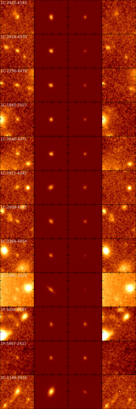
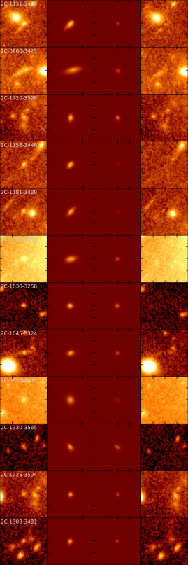
Figure 18.— Images for $z\sim 6-7$ faint galaxies at $M_{\mathrm{UV}}\gtrsim-18$. From left to right, $3^{\prime\prime}\times 3^{\prime\prime}$ cutout images, best-fit Sérsic profiles on the image plane, best-fit Sérsic profiles on the source plane, and residual images on the image plane.

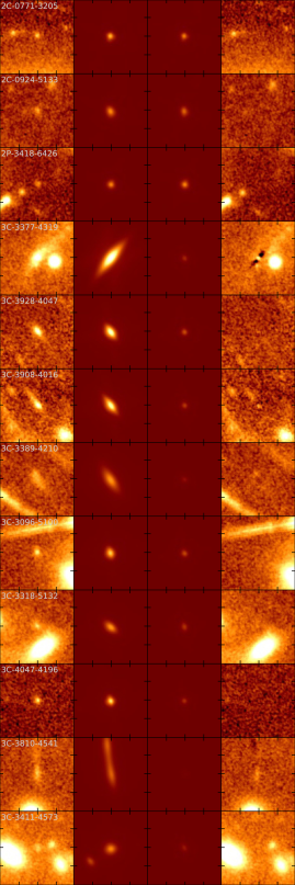
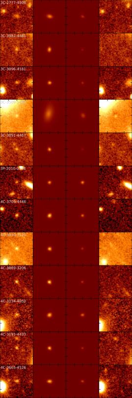
Figure 18.— Continued.

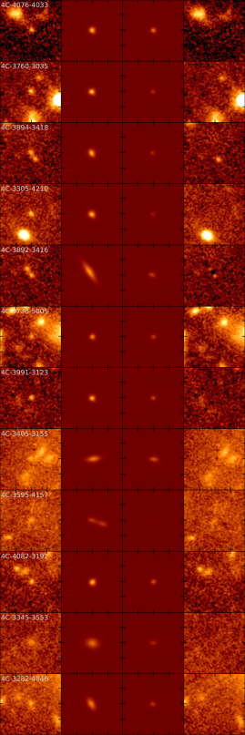
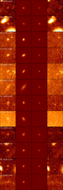
Figure 18.— Continued.

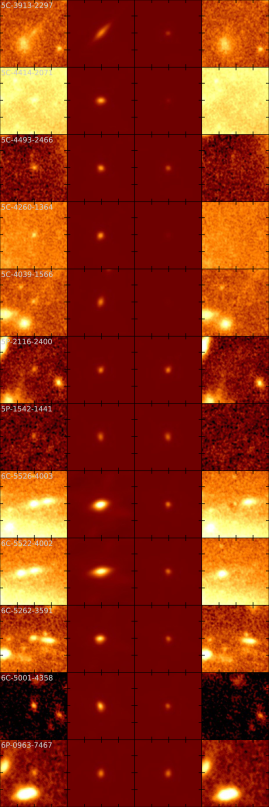
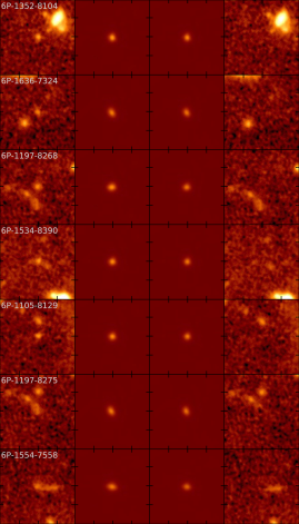
Figure 18.— Continued.

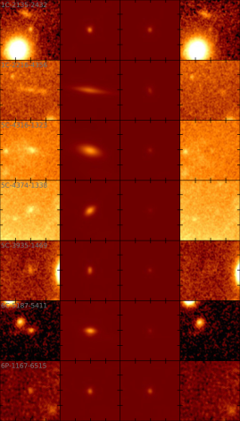
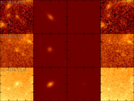
Figure 19.— Same as Figure 18 but for $z\sim 8$ (left) and $z\sim 9$ (right).

References

- Allen et al. (2017) Allen, R. J., Kacprzak, G. G., Glazebrook, K., et al. 2017, ApJ, 834, L11
- Atek et al. (2014) Atek, H., Richard, J., Kneib, J.-P., et al. 2014, ApJ, 786, 60
- Atek et al. (2015a) Atek, H., Richard, J., Jauzac, M., et al. 2015a, ApJ, 814, 69
- Atek et al. (2015b) Atek, H., Richard, J., Kneib, J.-P., et al. 2015b, ApJ, 800, 18
- Balestra et al. (2013) Balestra, I., Vanzella, E., Rosati, P., et al. 2013, A&A, 559, L9
- Behroozi et al. (2013) Behroozi, P. S., Wechsler, R. H., & Conroy, C. 2013, ApJ, 770, 57
- Benítez (2000) Benítez, N. 2000, ApJ, 536, 571
- Bertin & Arnouts (1996) Bertin, E., & Arnouts, S. 1996, A&AS, 117, 393
- Bertin et al. (2002) Bertin, E., Mellier, Y., Radovich, M., et al. 2002, in Astronomical Society of the Pacific Conference Series, Vol. 281, Astronomical Data Analysis Software and Systems XI, ed. D. A. Bohlender, D. Durand, & T. H. Handley, 228
- Bouwens et al. (2004) Bouwens, R. J., Illingworth, G. D., Blakeslee, J. P., Broadhurst, T. J., & Franx, M. 2004, ApJ, 611, L1
- Bouwens et al. (2017a) Bouwens, R. J., Illingworth, G. D., Oesch, P. A., et al. 2017a, ApJ, 843, 41
- Bouwens et al. (2017b) Bouwens, R. J., Oesch, P. A., Illingworth, G. D., Ellis, R. S., & Stefanon, M. 2017b, ApJ, 843, 129
- Bouwens et al. (2017c) Bouwens, R. J., van Dokkum, P. G., Illingworth, G. D., et al. 2017c, ArXiv e-prints, arXiv:1711.02090
- Bouwens et al. (2015) Bouwens, R. J., Illingworth, G. D., Oesch, P. A., et al. 2015, ApJ, 803, 34
- Bowler et al. (2017) Bowler, R. A. A., Dunlop, J. S., McLure, R. J., & McLeod, D. J. 2017, MNRAS, 466, 3612
- Boylan-Kolchin et al. (2009) Boylan-Kolchin, M., Springel, V., White, S. D. M., Jenkins, A., & Lemson, G. 2009, MNRAS, 398, 1150
- Brook et al. (2012) Brook, C. B., Stinson, G., Gibson, B. K., et al. 2012, MNRAS, 419, 771
- Brooks et al. (2011) Brooks, A. M., Solomon, A. R., Governato, F., et al. 2011, ApJ, 728, 51
- Bryan & Norman (1998) Bryan, G. L., & Norman, M. L. 1998, ApJ, 495, 80
- Bullock et al. (2001) Bullock, J. S., Kolatt, T. S., Sigad, Y., et al. 2001, MNRAS, 321, 559
- Caminha et al. (2016a) Caminha, G. B., Grillo, C., Rosati, P., et al. 2016a, A&A, 587, A80
- Caminha et al. (2016b) Caminha, G. B., Karman, W., Rosati, P., et al. 2016b, A&A, 595, A100
- Caminha et al. (2017) Caminha, G. B., Grillo, C., Rosati, P., et al. 2017, A&A, 600, A90
- Castellano et al. (2016) Castellano, M., Yue, B., Ferrara, A., et al. 2016, ApJ, 823, L40
- Charlton et al. (2017) Charlton, P. J. L., Hudson, M. J., Balogh, M. L., & Khatri, S. 2017, MNRAS, 472, 2367
- Christensen et al. (2012) Christensen, L., Richard, J., Hjorth, J., et al. 2012, MNRAS, 427, 1953
- Correa et al. (2015) Correa, C. A., Wyithe, J. S. B., Schaye, J., & Duffy, A. R. 2015, MNRAS, 452, 1217
- Curtis-Lake et al. (2016) Curtis-Lake, E., McLure, R. J., Dunlop, J. S., et al. 2016, MNRAS, 457, 440
- Danovich et al. (2015) Danovich, M., Dekel, A., Hahn, O., Ceverino, D., & Primack, J. 2015, MNRAS, 449, 2087
- Davis & Natarajan (2009) Davis, A. J., & Natarajan, P. 2009, MNRAS, 393, 1498
- de Jong & Lacey (2000) de Jong, R. S., & Lacey, C. 2000, ApJ, 545, 781
- Diego et al. (2015) Diego, J. M., Broadhurst, T., Molnar, S. M., Lam, D., & Lim, J. 2015, MNRAS, 447, 3130
- Diego et al. (2016a) Diego, J. M., Broadhurst, T., Wong, J., et al. 2016a, MNRAS, 459, 3447
- Diego et al. (2016b) Diego, J. M., Schmidt, K. B., Broadhurst, T., et al. 2016b, ArXiv e-prints, arXiv:1609.04822
- Ellis et al. (2013) Ellis, R. S., McLure, R. J., Dunlop, J. S., et al. 2013, ApJ, 763, L7
- Fall (1983) Fall, S. M. 1983, in IAU Symposium, Vol. 100, Internal Kinematics and Dynamics of Galaxies, ed. E. Athanassoula, 391–398
- Fall & Efstathiou (1980) Fall, S. M., & Efstathiou, G. 1980, MNRAS, 193, 189
- Fall & Romanowsky (2013) Fall, S. M., & Romanowsky, A. J. 2013, ApJ, 769, L26
- Ferguson et al. (2004) Ferguson, H. C., Dickinson, M., Giavalisco, M., et al. 2004, ApJ, 600, L107
- Foreman-Mackey (2016) Foreman-Mackey, D. 2016, The Journal of Open Source Software, 24, 1
- Foreman-Mackey et al. (2013) Foreman-Mackey, D., Hogg, D. W., Lang, D., & Goodman, J. 2013, PASP, 125, 306
- Genel et al. (2015) Genel, S., Fall, S. M., Hernquist, L., et al. 2015, ApJ, 804, L40
- González et al. (2011) González, V., Labbé, I., Bouwens, R. J., et al. 2011, ApJ, 735, L34
- Grazian et al. (2011) Grazian, A., Castellano, M., Koekemoer, A. M., et al. 2011, A&A, 532, A33
- Grazian et al. (2012) Grazian, A., Castellano, M., Fontana, A., et al. 2012, A&A, 547, A51
- Grillo et al. (2015) Grillo, C., Suyu, S. H., Rosati, P., et al. 2015, ApJ, 800, 38
- Grogin et al. (2011) Grogin, N. A., Kocevski, D. D., Faber, S. M., et al. 2011, ApJS, 197, 35
- Guo et al. (2016) Guo, Q., Gonzalez-Perez, V., Guo, Q., et al. 2016, MNRAS, 461, 3457
- Henriques et al. (2015) Henriques, B. M. B., White, S. D. M., Thomas, P. A., et al. 2015, MNRAS, 451, 2663
- Hoag et al. (2016) Hoag, A., Huang, K.-H., Treu, T., et al. 2016, ApJ, 831, 182
- Holwerda et al. (2015) Holwerda, B. W., Bouwens, R., Oesch, P., et al. 2015, ApJ, 808, 6
- Hou et al. (2017) Hou, J., Lacey, C. G., & Frenk, C. S. 2017, ArXiv e-prints, arXiv:1708.02950
- Huang et al. (2013) Huang, K.-H., Ferguson, H. C., Ravindranath, S., & Su, J. 2013, ApJ, 765, 68
- Huang et al. (2017) Huang, K.-H., Fall, S. M., Ferguson, H. C., et al. 2017, ApJ, 838, 6
- Illingworth et al. (2013) Illingworth, G. D., Magee, D., Oesch, P. A., et al. 2013, ApJS, 209, 6
- Ishigaki et al. (2015) Ishigaki, M., Kawamata, R., Ouchi, M., et al. 2015, ApJ, 799, 12
- Ishigaki et al. (2018) —. 2018, ApJ, 854, 73
- Jauzac et al. (2014) Jauzac, M., Clément, B., Limousin, M., et al. 2014, MNRAS, 443, 1549
- Jauzac et al. (2015) Jauzac, M., Richard, J., Jullo, E., et al. 2015, MNRAS, 452, 1437
- Jiang et al. (2013) Jiang, L., Egami, E., Fan, X., et al. 2013, ApJ, 773, 153
- Johnson et al. (2014) Johnson, T. L., Sharon, K., Bayliss, M. B., et al. 2014, ApJ, 797, 48
- Karman et al. (2015) Karman, W., Caputi, K. I., Grillo, C., et al. 2015, A&A, 574, A11
- Karman et al. (2017) Karman, W., Caputi, K. I., Caminha, G. B., et al. 2017, A&A, 599, A28
- Kawamata et al. (2015) Kawamata, R., Ishigaki, M., Shimasaku, K., Oguri, M., & Ouchi, M. 2015, ApJ, 804, 103
- Kawamata et al. (2016) Kawamata, R., Oguri, M., Ishigaki, M., Shimasaku, K., & Ouchi, M. 2016, ApJ, 819, 114
- Koekemoer et al. (2011) Koekemoer, A. M., Faber, S. M., Ferguson, H. C., et al. 2011, ApJS, 197, 36
- Koekemoer et al. (2013) Koekemoer, A. M., Ellis, R. S., McLure, R. J., et al. 2013, ApJS, 209, 3
- Lagattuta et al. (2017) Lagattuta, D. J., Richard, J., Clément, B., et al. 2017, MNRAS, 469, 3946
- Lam et al. (2014) Lam, D., Broadhurst, T., Diego, J. M., et al. 2014, ApJ, 797, 98
- Laporte et al. (2016) Laporte, N., Infante, L., Troncoso Iribarren, P., et al. 2016, ApJ, 820, 98
- Liu et al. (2017) Liu, C., Mutch, S. J., Poole, G. B., et al. 2017, MNRAS, 465, 3134
- Livermore et al. (2017) Livermore, R. C., Finkelstein, S. L., & Lotz, J. M. 2017, ApJ, 835, 113
- Lotz et al. (2017) Lotz, J. M., Koekemoer, A., Coe, D., et al. 2017, ApJ, 837, 97
- Ma et al. (2017) Ma, X., Hopkins, P. F., Boylan-Kolchin, M., et al. 2017, ArXiv e-prints, arXiv:1710.00008
- Mahler et al. (2018) Mahler, G., Richard, J., Clément, B., et al. 2018, MNRAS, 473, 663
- McLeod et al. (2015) McLeod, D. J., McLure, R. J., Dunlop, J. S., et al. 2015, MNRAS, 450, 3032
- Meneghetti et al. (2017) Meneghetti, M., Natarajan, P., Coe, D., et al. 2017, MNRAS, 472, 3177
- Merten et al. (2011) Merten, J., Coe, D., Dupke, R., et al. 2011, MNRAS, 417, 333
- Mo et al. (1998) Mo, H. J., Mao, S., & White, S. D. M. 1998, MNRAS, 295, 319
- Monna et al. (2014) Monna, A., Seitz, S., Greisel, N., et al. 2014, MNRAS, 438, 1417
- Mutch et al. (2016) Mutch, S. J., Geil, P. M., Poole, G. B., et al. 2016, MNRAS, 462, 250
- Oesch et al. (2010a) Oesch, P. A., Bouwens, R. J., Carollo, C. M., et al. 2010a, ApJ, 709, L21
- Oesch et al. (2010b) Oesch, P. A., Bouwens, R. J., Illingworth, G. D., et al. 2010b, ApJ, 709, L16
- Oesch et al. (2013) —. 2013, ApJ, 773, 75
- Oguri (2010) Oguri, M. 2010, PASJ, 62, 1017
- Okamura et al. (2018) Okamura, T., Shimasaku, K., & Kawamata, R. 2018, ApJ, 854, 22
- Oke & Gunn (1983) Oke, J. B., & Gunn, J. E. 1983, ApJ, 266, 713
- Ono et al. (2013) Ono, Y., Ouchi, M., Curtis-Lake, E., et al. 2013, ApJ, 777, 155
- Ono et al. (2017) Ono, Y., Ouchi, M., Harikane, Y., et al. 2017, ArXiv e-prints, arXiv:1704.06004
- Peebles (1969) Peebles, P. J. E. 1969, ApJ, 155, 393
- Peng et al. (2002) Peng, C. Y., Ho, L. C., Impey, C. D., & Rix, H.-W. 2002, AJ, 124, 266
- Peng et al. (2010) —. 2010, AJ, 139, 2097
- Postman et al. (2012) Postman, M., Coe, D., Benítez, N., et al. 2012, ApJS, 199, 25
- Prada et al. (2012) Prada, F., Klypin, A. A., Cuesta, A. J., Betancort-Rijo, J. E., & Primack, J. 2012, MNRAS, 423, 3018
- Priewe et al. (2017) Priewe, J., Williams, L. L. R., Liesenborgs, J., Coe, D., & Rodney, S. A. 2017, MNRAS, 465, 1030
- Reddy & Steidel (2009) Reddy, N. A., & Steidel, C. C. 2009, ApJ, 692, 778
- Richard et al. (2010) Richard, J., Kneib, J.-P., Limousin, M., Edge, A., & Jullo, E. 2010, MNRAS, 402, L44
- Richard et al. (2014) Richard, J., Jauzac, M., Limousin, M., et al. 2014, MNRAS, 444, 268
- Roche et al. (1996) Roche, N., Ratnatunga, K., Griffiths, R. E., Im, M., & Neuschaefer, L. 1996, MNRAS, 282, 1247
- Rodney et al. (2017) Rodney, S. A., Balestra, I., Bradac, M., et al. 2017, ArXiv e-prints, arXiv:1707.02434
- Romanowsky & Fall (2012) Romanowsky, A. J., & Fall, S. M. 2012, ApJS, 203, 17
- Sales et al. (2010) Sales, L. V., Navarro, J. F., Schaye, J., et al. 2010, MNRAS, 409, 1541
- Schmidt et al. (2014a) Schmidt, K. B., Treu, T., Trenti, M., et al. 2014a, ApJ, 786, 57
- Schmidt et al. (2014b) Schmidt, K. B., Treu, T., Brammer, G. B., et al. 2014b, ApJ, 782, L36
- Shen et al. (2003) Shen, S., Mo, H. J., White, S. D. M., et al. 2003, MNRAS, 343, 978
- Shibuya et al. (2015) Shibuya, T., Ouchi, M., & Harikane, Y. 2015, ApJS, 219, 15
- Somerville et al. (2017) Somerville, R. S., Behroozi, P., Pandya, V., et al. 2017, ArXiv e-prints, arXiv:1701.03526
- Springel et al. (2005) Springel, V., White, S. D. M., Jenkins, A., et al. 2005, Nature, 435, 629
- Steidel et al. (1999) Steidel, C. C., Adelberger, K. L., Giavalisco, M., Dickinson, M., & Pettini, M. 1999, ApJ, 519, 1
- Treu et al. (2015) Treu, T., Schmidt, K. B., Brammer, G. B., et al. 2015, ApJ, 812, 114
- Vitvitska et al. (2002) Vitvitska, M., Klypin, A. A., Kravtsov, A. V., et al. 2002, ApJ, 581, 799
- Wang et al. (2015) Wang, X., Hoag, A., Huang, K.-H., et al. 2015, ApJ, 811, 29
- Wyithe & Loeb (2011) Wyithe, J. S. B., & Loeb, A. 2011, MNRAS, 413, L38
- Yue et al. (2017) Yue, B., Castellano, M., Ferrara, A., et al. 2017, ArXiv e-prints, arXiv:1711.05130
- Zitrin et al. (2013) Zitrin, A., Meneghetti, M., Umetsu, K., et al. 2013, ApJ, 762, L30
- Zitrin et al. (2014) Zitrin, A., Zheng, W., Broadhurst, T., et al. 2014, ApJ, 793, L12
- Zjupa & Springel (2017) Zjupa, J., & Springel, V. 2017, MNRAS, 466, 1625