Clustering the Orion B giant molecular cloud based on its molecular emission
Abstract
Context. Previous attempts at segmenting molecular line maps of molecular clouds have focused on using position-position-velocity data cubes of a single molecular line to separate the spatial components of the cloud. In contrast, wide field spectral imaging over a large spectral bandwidth in the (sub)mm domain now allows one to combine multiple molecular tracers to understand the different physical and chemical phases that constitute giant molecular clouds (GMCs).
Aims. We aim at using multiple tracers (sensitive to different physical processes and conditions) to segment a molecular cloud into physically/chemically similar regions (rather than spatially connected components), thus disentangling the different physical/chemical phases present in the cloud.
Methods. We use a machine learning clustering method, namely the Meanshift algorithm, to cluster pixels with similar molecular emission, ignoring spatial information. Clusters are defined around each maximum of the multidimensional Probability Density Function (PDF) of the line integrated intensities. Simple radiative transfer models were used to interpret the astrophysical information uncovered by the clustering analysis.
Results. A clustering analysis based only on the lines of three isotopologues of CO proves sufficient to reveal distinct density/column density regimes (, , and ), closely related to the usual definitions of diffuse, translucent and high-column-density regions. Adding two UV-sensitive tracers, the line of HCO+ and the line of CN, allows us to distinguish two clearly distinct chemical regimes, characteristic of UV-illuminated and UV-shielded gas. The UV-illuminated regime shows overbright HCO+ and CN emission, which we relate to a photochemical enrichment effect. We also find a tail of high CN/HCO+ intensity ratio in UV-illuminated regions. Finer distinctions in density classes (, ) for the densest regions are also identified, likely related to the higher critical density of the CN and HCO+ lines. These distinctions are only possible because the high-density regions are spatially resolved.
Conclusions. Molecules are versatile tracers of GMCs because their line intensities bear the signature of the physics and chemistry at play in the gas. The association of simultaneous multi-line, wide-field mapping and powerful machine learning methods such as the Meanshift clustering algorithm reveals how to decode the complex information available in these molecular tracers.
Key Words.:
Astrochemistry, ISM: molecules, ISM: clouds, ISM: structure, Object: Orion B, Methods: statistical1 Introduction
The inter-stellar medium (ISM) is made of several physical/chemical phases: dense versus diffuse gas, hot versus cold gas, ionised, atomic, or molecular gas, FUV-illuminated versus FUV-shielded gas, and gravitationally bound versus free-floating gas. The ISM molecular composition is particularly sensitive to the changes that affect the gas and dust when they cycle between these different phases. Wide-field mapping of the line emission of many molecules sensitive to different physical processes could thus enable one to segment giant molecular clouds (GMCs) into regions belonging to distinct physical/chemical phases, so that we can then study the physics and chemistry of these regions in detail. Moreover, understanding the prevalence of these different phases inside a given molecular cloud, and learning how to disentangle their relative contributions to each molecular tracer is of interest to interpret the spatially unresolved molecular emission in extragalactic studies.
The advent of wide-band high-spectral-resolution spectrometers associated to future multi-beam receivers in the (sub-)millimetre domain will enable radio-astronomers to easily map the emission of many lines from tens of species over tens of square degrees on the sky. The pioneer ORION-B project (Outstanding Radio-Imaging of OrioN-B, PI: J. Pety and M. Gerin) currently uses the IRAM-30m/EMIR spectrometer to image about 4.5 square degrees of the Southern part of the Orion B molecular cloud at typical spectral resolutions of and an angular resolution of (i.e. or at the distance of Orion B: 400, Menten et al. 2007; Schlafly et al. 2014) and a typical sensitivity of over almost all of the 3 mm atmospheric window.
This paper is part of the first series of papers based on the already acquired dataset that covers about 1 square degree of the Orion B molecular cloud surrounding the Horsehead nebula, NGC 2023, and NGC 2024, in the frequency range. Pety et al. (2017) introduce the molecular anatomy of the Orion B GMC, including relationships between line intensities and gas column density or far-UV radiation field, and correlations between selected lines and line ratios. They obtain a dust-traced gas mass that is less than approximately one third of the CO-traced mass, using the standard conversion factor. The presence of overluminous CO can be traced back to the dependence of the CO intensity on the gas kinetic temperature, which in turn is affected by the FUV illumination (photo-electric heating). While most lines show some dependence on the UV radiation field, CN and are found to be the most sensitive. Moreover, dense cloud cores are almost exclusively traced by . Other traditional high-density tracers, such as HCN(1-0) or HCO+(1-0), are also easily detected in extended translucent regions at a typical density of about . Gratier et al. (2017) propose a first multi-line approach applying Principal Component Analysis (PCA, Jolliffe 2002) on 12 of the brightest lines (integrated over a narrow velocity range) to reveal the pattern of correlations between the different tracers. This approach emphasises three clear trends: 1) the line intensities are well correlated with the column density, that is, the more matter along the line of sight, the brighter the lines; 2) CCH, CN, HCN are correlated with the FUV ( eV) irradiation (while and the CO isotopologues are anti-correlated); and 3) the PCA method confirms the known anticorrelation between and CO in dense cores. Finally, the 13CO position-position-velocity cube has been used by Orkisz et al. (2017) to show that solenoidal motions clearly dominate over the observed field of view, in agreement with the low star formation efficiency measured in Orion B (Lada 1992; Carpenter 2000; Megeath et al. 2016).
In this paper, we take a further step to characterise the different ISM phases from a multi-line wide-field dataset. The basic idea is similar to remote sensing in Earth studies (e.g. Inglada et al. 2017) which tries to classify environments (forests, deserts, mountains, oceans, etc.), based on the dominant colour they emit. In other words, we wish to segment the dataset into a small (yet unknown) number of classes that have a well defined physical or chemical meaning, based on their molecular emission. This goal requires the use of data-mining techniques in order to go beyond a tracer-by-tracer analysis, and take advantage of the full information hidden in the joint variations of the different tracers. Classification techniques are divided into two categories. Supervised ones use known examples of the desired classes to learn how to automatically classify new observations. They thus require a priori independent knowledge of the physical or chemical properties of the different ISM phases. These approaches will be explored in future papers. In contrast, clustering, which is an unsupervised technique, aims to reveal how the data points naturally group themselves into distinct clusters of points with similar properties, hinting at the existence of different physical or chemical regimes. This is the approach that we adopt in this paper.
Traditional segmentation approaches in GMC studies typically segment the map of emission of a single tracer into constitutive clumps (Stutzki & Guesten 1990; Williams et al. 1994; Rosolowsky & Leroy 2006; Colombo et al. 2015). These methods use in one way or another the topology (contiguity) of the emission in the position-position-velocity space, sometimes associated with additional physical properties such as the virial state. Their goal is thus to separate the spatial components of a GMC. In contrast, we here propose to work on multi-dimensional Probability Density Distributions (PDFs) of the line integrated intensities. The PDF shape can indeed show distinct components, which can reveal distinct physical/chemical regimes, and which we want to automatically separate. For instance, in the Hertzprung-Russell (HR) diagram, different branches in the colour versus magnitude plot correspond to different stages of stellar evolution (main sequence, giant branch, etc.). However, while recognising structure by eye is possible in two-dimensional (2D) datasets, direct visualisation of the data becomes difficult in higher dimension. Simple 2D projections for each pair of line intensities do not necessary reveal all the existing structure, and clustering algorithms become necessary. In the case of the ORION-B dataset, Gratier et al. (2017) show that understanding the physics and chemistry underlying the extended molecular line emission requires a multi-dimensional analysis of the data. To our knowledge, clustering a GMC based on its (multi-molecule) molecular emission similarity rather than spatial (or PPV) contiguity has never been done before.
This paper is organised as follows. In Sect. 2, we present the data used in our analysis. We then explain the clustering algorithm that we chose to use in Sect. 3. This clustering method is first applied to the most widely observed lines in the millimetre wave domain, that is, the lines of three CO isotopologues (, and ) in Sect. 4. Sect. 5 then discusses the additional results obtained when adding the ground-state transitions of HCO+ and CN to the analysis, whose intensities are known to be related to the FUV illumination. We discuss the benefits and limits of the method in Sect. 6. We present our conclusions in Sect. 7.
2 Data
2.1 IRAM-30m observations
Pety et al. (2017) present in detail the acquisition and data reduction of the dataset used in this study. In short, the data were acquired at the IRAM-30m telescope by the ORION-B project from August 2013 to November 2014. The frequency range from 84 to 116 was completely sampled at 200 spectral resolution. Such a large bandwidth allowed us to image over 20 chemical species at a median sensitivity of 0.1 (main-beam temperature) per channel. As opposed to several small bandwidth mappings, the spectral lines in this survey are observed in only two tunings covering 16 each. They are thus well inter-calibrated, which gives an unprecedented spectral accuracy for such a large field of view. The intensity dynamic range reaches .
The field of view presented covers towards the Orion B molecular cloud part that contains the Horsehead nebula, and the Hii regions NGC 2023, NGC 2024, IC 434, and IC 435. The angular resolution ranges from 22.5 to . The position-position-velocity cubes of each line were smoothed at a common angular resolution of to avoid resolution effects during the comparison. At a distance of 400 (Menten et al. 2007), the sampled linear scales range from to .
The observations provided a position-position-frequency cube of pixels, each pixel covering (Nyquist sampling at the highest frequency, i.e.(1–0) at 115.27).
We here study maps of line integrated intensities. Lines are detected over quite different velocity ranges. Using a large velocity range would artificially increase the noise for most of the lines, while adapting the velocity range to each line could bias the comparisons. We thus focus on a narrow velocity range where the bulk of the gas emits. While Gratier et al. (2017) computed for each line the mean of three velocity channels around 10.5, we use here a more common radioastronomical approach, which is to integrate the line intensity profile. We here integrate over the velocity interval where the main velocity component of the Orion B cloud sits (see section 2.5 of Pety et al. 2017). To first order, both sets of maps are proportional to one another (the respective velocity ranges differ slightly)111The data products associated with this paper are available at http://www.iram.fr/~pety/ORION-B.
2.2 Herschel observations
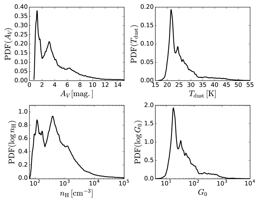
In order to get independent constraints on the physical conditions in the Orion B cloud, we use the dust continuum observations from the Herschel Gould Belt Survey (André et al. 2010; Schneider et al. 2013) and from the Planck satellite (Planck Collaboration et al. 2011). The fit of the spectral energy distribution by Lombardi et al. (2014) gives us access to the spatial distributions of the dust opacity at and of the dust temperature. As in Pety et al. (2017), we converted to visual extinctions using . The top panels of Fig. 1 show the PDF of the dust visual extinction and temperature.
The PDF shows three distinct peaks, indicating that the field of view samples three different regimes: , , and . These regimes are consistent with the usual distinction between diffuse, translucent, and high-column-density regions (Snow & McCall 2006). As in Pety et al. (2017), we use as conversion factor between visual extinction and hydrogen column density: . In addition, we propose a conversion from the column density to an approximate volume density map. The procedure is discussed in detail in Appendix A. In summary, we assume a rough isotropy of the cloud (similar dimensions along the line of sight and in the plane of the sky) to deduce an estimate of the average hydrogen density along each line of sight as follows. For a given column density value , we consider the region where . We then estimate the line-of-sight depth of this region from its plane-of-the-sky surface as (using our isotropy assumption). We finally assign the approximate volume density to the pixels where .
The resulting approximate volume density PDF is shown in the bottom-left panel of Fig. 1. The three distinct regimes correspond to three volume density regimes: one low-density peak close to corresponds to diffuse gas, a second peak covering the range is associated to the translucent gas, and a third smaller peak slightly above with a long tail extending up to a few corresponds to denser gas. The values found after our conversion are consistent with the usual orders of magnitude for diffuse, translucent, and denser gas. More quantitatively, Appendix A shows that our estimation of the volume density is valid in a statistical way with a bias of a factor of 3 at most and a typical scatter of one order of magnitude, when compared with volume density estimates from the literature that make different hypotheses. The deduced values of are rough estimates that should not be trusted beyond order-of-magnitude comparisons. However, this method reproduces the observed range of densities fairly well, indicating that the shape of the PDF is also approximately correct.
The PDF shows a less marked multi-peak structure with a sharp first peak at , a small secondary peak at and a shallow third peak at . A first steep tail extends up to , followed by a second flatter tail (reaching values up to ). These two tails are indicative of highly FUV-illuminated regions. Pety et al. (2017) converted the dust temperature map into an approximate map of the far ultra-violet radiation field in units of the Habing Interstellar Standard Radiation Field (ISRF, Habing 1968), using the simple approximation of Hollenbach et al. (1991)
| (1) |
Shimajiri et al. (2017) compared this estimation with another estimation directly using the far infra-red intensities at 70 and . Both estimates agree within 30%. The PDF of is shown as the bottom right panel of Fig. 1 and is very similar to the dust temperature PDF (as the conversion is a simple power law). As mentioned before, the main peak is close to 20 times the ISRF while the tail extends up to several thousand times the ISRF. As for our estimate of , the deduced values of should only be trusted at order-of-magnitude levels.
3 The Meanshift clustering method
From a mathematical viewpoint, the data are a set of points characterised by their two sky coordinates and the integrated intensities of molecular lines. The dataset thus lies in a space of dimensions. As discussed before, we aim to cluster the datapoints based on their molecular emission only, and not their spatial proximity. For clarity, we thus separate the data space into two parts: 1) the usual position space, and 2) the line space of dimension spanned by the molecular line intensities. Clustering will only be done in the line space, ignoring the location of the pixels in the position space. After a non-exhaustive discussion of methods that segment the data based on their multi-dimensional PDF, we describe the Meanshift algorithm and the implementation used in this paper.
3.1 The two families of PDF-based clustering methods
We are interested in clustering methods that aim to separate components in the (multi-dimensional) PDF of the data. Two families of such methods can be defined. The first family assumes that the data PDF can naturally be decomposed into components of some given functional form, for example, Gaussian functions, controlled by free parameters. These methods are thus called parametric approaches. The complete dataset is assumed to be a mixture of several components, with the same functional form but different values for the control parameters. These algorithms are thus usually called mixture models (see Bishop 2006, Chap. 9). This approach has two main drawbacks. First, the number of free parameters tends to increase quickly with the dimension of the problem, resulting in a difficult and often degenerate optimisation. To alleviate this problem, restrictions are imposed on the free parameters. For instance, assuming Gaussian components and forcing them to all have the same scalar covariance matrix (thus forcing spherically symmetric clusters of equal size) yields the K-means algorithm, one of the most used clustering algorithms. Second, the assumption of a functional PDF form is a strong a priori that can bias the clustering when this form is inadequate for the studied data. More flexible functional forms reduce this problem but result in more free parameters. In this family, a compromise has to be made between the flexibility of the assumed functional PDF form and the number of free parameters.
The second family takes a data-driven approach, by defining clusters around local maxima of the data PDF. Each cluster is thus a region of high density in the line space, separated from the other clusters by regions of lower density. This definition has two advantages: 1) It allows to capture any shape of the PDF of the clusters (possibly curved and elongated); 2) The number of clusters is determined automatically from the data. Data clusters must however create a maximum in the PDF to be detected. A small group of datapoints blended in the tail of another more common cluster might thus not be detected. The two most famous algorithms in this family take a different approach to finding the high-density regions in the line space. First, the DBSCAN algorithm (Ester et al. 1996) uses a graph-based approach to find high-density regions, but it assumes a similar density of points inside all clusters. Second, the Meanshift algorithm (Comaniciu & Meer 2002) searches for the maxima of the data PDF using a kernel-based approach. We choose to use the Meanshift approach, as it can detect clusters that have both different sizes and different densities. Moreover, its direct link to the data PDF eases the interpretation of the clusters. The following Section describes this algorithm in detail.
3.2 The Meanshift algorithm
3.2.1 General description
The Meanshift algorithm (see Comaniciu & Meer 2002 for more details) associates each data point to the closest local maximum of some empirical estimate of the PDF. The algorithm iteratively climbs up the slope of the PDF starting from each of the datapoints. The set of datapoints converging to the same PDF maximum constitutes a cluster.
The algorithm is based on the same concept as the Kernel Density Estimate method (Rosenblatt 1956; Parzen 1962), which estimates the PDF of a random variable (here, the intensities) from one sample realisation. The kernel density estimator for a given set of -dimensional data points is
| (2) |
where is a distance in the line space between a given a vector and the vector associated to the th datapoint (both are vectors of line intensities), is the smoothing kernel (a non-negative decreasing function of ), is the bandwidth of the smoothing and a normalisation constant. The kernel often has a finite support , so that the estimation of the PDF at is only based on the datapoints that are closer to than the bandwidth .
The Meanshift algorithm avoids the estimation of the PDF itself by directly estimating the PDF gradient with the same kernel smoothing approach. By taking the gradient of Eq. 2 in the case of an Euclidean distance, and noting , which is a new kernel, we obtain
| (3) |
| (4) |
which is called the Mean Shift vector as it gives the shift from the current position to the mean of the datapoints weighted by the kernel centered on . Equation 3 indicates that this Mean Shift vector gives an estimate of the relative gradient (the local PDF gradient divided by the local PDF).
The following iterative algorithm is applied, starting from each of the datapoints:
-
•
Compute the Mean Shift vector at the current estimate of the searched local maxima.
-
•
Modify the current estimate by shifting it by the Mean Shift vector.
This algorithm converges to points where the PDF gradient estimate is zero, and that usually are local maxima due to its hill climbing nature. Convergence points that are closer to each other than the bandwidth are then merged, and clusters are defined as the sets of datapoints that have converged to the same extremum. Data points lying close to local minima can sometimes stay stuck due to the associated null gradient, but the resulting unwanted clusters can easily be recognised by the very small number of datapoints they contain, and removed by assigning their datapoints to the closest clusters.
3.2.2 The FAMS implementation
In this article, we used the Fast Adaptive Mean Shift (FAMS) code described in Georgescu et al. (2003), and provided by the authors on their webpage222 http://coewww.rutgers.edu/riul/research/code/AMS/index.html. This code implements several modifications to the Meanshift principle in order to improve the quality of the gradient estimate in low-density regions.
The quality of the PDF gradient estimate depends on the number of datapoints present inside the smoothing kernel. Consequently, using a fixed bandwidth results in insufficiently sampled gradient estimates in the tails of the data PDF. This leads to many artificial maxima being found in these tails, unless the bandwidth is increased. But the central parts of the PDF then risk being overly smoothed and significant maxima can be lost. To alleviate this problem, Comaniciu et al. (2001) proposed an adaptive-bandwidth Meanshift algorithm, in which a different bandwidth is assigned to each data point ( is replaced by in Eq. 4). The Adaptive Meanshift Algorithm uses the simplest method to choose the bandwidth for each datapoint: taking the distance to the -nearest neighbour to the datapoint as the bandwidth, so that there is always roughly the same number of datapoints inside the kernel. This number of neighbours becomes a parameter of the method to be adjusted by the user (instead of the bandwidth value in the classical Meanshift algorithm). In other words, there is a trade-off between the sampling variance and the smoothing factor to estimate the PDF: an adaptive smoothing is applied so that low-density regions are smoothed on a larger scale than high-density regions. All estimates of the PDF gradient are then equally well sampled.
Second, the FAMS implementation uses a distance () instead of the usual Euclidean distance (). This allows for an additional optimisation in high dimension (Georgescu et al. 2003); but it is only an approximation of the Meanshift algorithm, as Eq. 4 assumes a Euclidean distance. Finally, the kernel used in this implementation is .
3.2.3 In practice
The main control parameter of the Meanshift algorithm is either the bandwidth value when using the fixed bandwidth implementation or the number of nearest neighbours when using the adaptative bandwidth version. This parameter controls the scale on which the PDF is smoothed in both cases. We use here the adaptive bandwidth version. In each studied case, was varied from a few hundred to a few thousand, and adjusted to increase or decrease the number of clusters found. Any cluster that contains a number of pixels that is very small compared to is merged with the closest cluster. This can happen when the Meanshift algorithm is stuck into a local minimum of the PDF.
The smoothing part uses a spherical kernel, so that the applied smoothing is isotropic, that is, it has the same absolute bandwidth in all directions. It is thus necessary to ensure that the variability of the dataset along the different dimensions (that is the intensity dynamic of each line) is comparable. Without a linear rescaling, either the variations of the faint lines would be smoothed out by a bandwidth adapted to the bright lines or the bright lines would drive the segmentation into many small clusters when using a bandwidth adapted to the faint lines. We thus standardised the dataset (we ensured that the intensity PDF of each line has a unit standard deviation) before applying the Meanshift algorithm. Additional non-linear transformations applied to the dataset before clustering it with Meanshift would in general modify the number and positions of PDF maxima and thus affect the results. As we wish to check the amount of physical/chemical information encoded in the line intensities, we chose to only linearly standardise the data.
The clustering of our data points with , and , typically takes 10 to 20 hours of computation on a single standard CPU in 2017. Taking into account that our data has some redundancy (Nyquist sampling), we tested the method on a decimated dataset before getting the final results on the full dataset.
Comaniciu et al. (2001) showed that adding spatial coordinates in addition to intensities when clustering images may smooth the resulting clusters. We did not use the spatial information present in our dataset, as our focus is on grouping pixels where the intensities are similar rather that pixels belonging to the same spatial structure. We will however use the spatial coherence of the clusters found as a consistency check of the results because some amount of physical/chemical similarity is expected between neighbouring pixels.
When discussing the results, we visualise the 2D PDFs of pairs of lines (comparing the contributions of the obtained clusters) using kernel density estimation (Rosenblatt 1956; Parzen 1962) from the scikit-learn Python package (Pedregosa et al. 2011), with an Epanechnikov kernel (, optimal in terms of mean squared error, Epanechnikov 1969). This implementation uses a fixed bandwidth. This is however only used as a visualisation tool, and is independent of our Meanshift clustering analysis.
4 The CO isotopologue emission enables us to separate the diffuse, translucent, and denser gas regimes
The , , and lines are amongst the most observed radio lines in molecular clouds. At constant elemental ratios of the carbon isotopes, the naive chemical interpretation suggests that the relative abundances of these three species should be identical in all lines of sight of a GMC. Moreover, the critical densities of these three lines for collisional excitation with H2 are similar (), implying similar excitation conditions. Differences in optical depths should therefore be the main factor governing the intensity ratios. In this Section, we ask whether or not clustering the intensities of these lines can distinguish physical regimes known to happen in the studied field of view. We thus first apply the Meanshift algorithm to a dataset consisting of the maps of the lines of 12CO, 13CO and C18O only (, ).
After several trials for the number of neighbours in the adaptive kernel width, we chose a compromise between avoiding picking up sampling fluctuations in the PDF as artificial maxima and smoothing out physical maxima of interest (see Appendix B for a discussion of this choice). We settled on neighbours. In order to understand and interpret the clustering, we present in the following the spatial distribution of the clusters as well as PDFs of 1D or 2D projections of the data (that is, PDFs of single lines or pairs of lines).
4.1 Spatial distribution
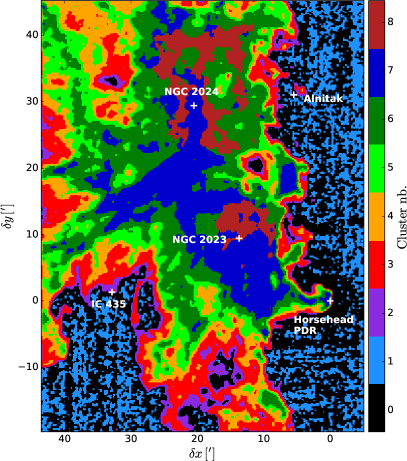
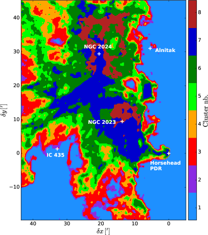
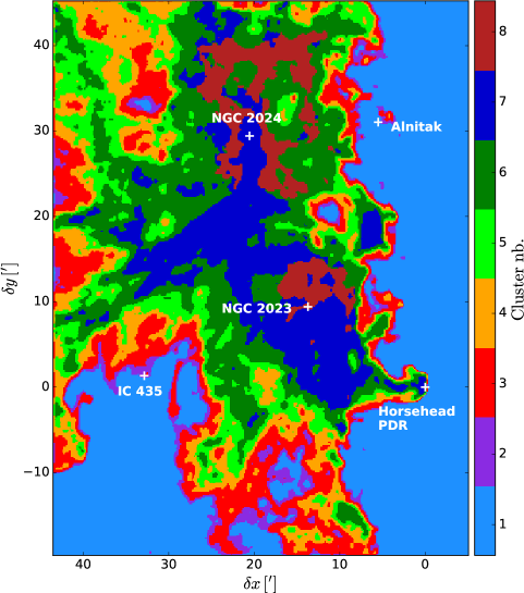
We find nine clusters, whose spatial distribution is shown in Fig. 2. For the following discussion, we name these clusters CO-0 to CO-8. While our use of the Meanshift clustering does not take into account the spatial contiguity, they show very consistent spatial distributions, except for clusters CO-0 and CO-1 which share the outer region of the cloud and display a noise-like pattern. A visual inspection of the CO isotopologue PDFs shows that this distinction most likely comes from noise properties. We thus merge cluster CO-0 with cluster CO-1. We call the new cluster CO-1 and represent it in light blue. The resulting cluster map is shown on the right panel of Fig. 2.
Clusters CO-1 to CO-7 show a nested pattern highlighting successive layers from the surface to the inner parts of the cloud. These clusters are present both on the eastern and western sides that surround the inner region of the imaged field of view. However, an asymmetry between the two sides is visible in the much smaller thickness of the surface layers highlighted by the transition from clusters CO-2 to CO-5 on the western FUV-illuminated side. This is a consequence of the much steeper intensity gradients for all three CO lines on this side of the cloud. In other words, high FUV illumination has a much stronger impact on the CO intensity gradients than on the intensities themselves. Cluster CO-8 differs as it only appears towards the two Hii regions, NGC 2023 and NGC 2024, which are embedded in the south-western part of Orion B.
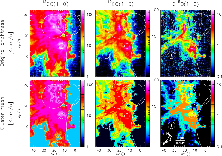
One way to check the quality of the clustering is to compare the spatial distributions of the original line intensities with the line intensities averaged in each cluster. This is somehow a test of the ability of the clustering method to compress the information contained in the line intensity maps while retaining the most important aspects. Taking the mean of the line intensities for each cluster conserves the total flux in the output images. Figure 3 presents such a comparison. The mean intensities (and other characteristic intensity values) of each line in each cluster are listed in Table C. Most of the and spatial features are preserved in the clustered images, while the representation of the image is not as good: some spatial features appear and others disappear. This comparison also highlights that cluster CO-8 is characterised by an increased intensity compared to its surrounding. We can note that the Horsehead pillar and the other dense clumps that emerge from the IC 434 Hii region belong to cluster CO-7 which is associated with relatively dense gas (as discussed in the following subsections).
4.2 Projected PDFs
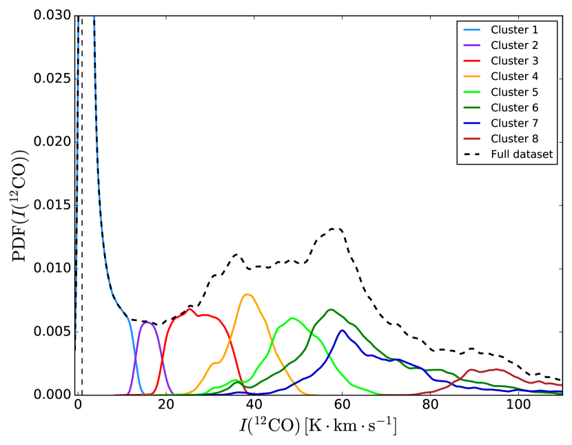
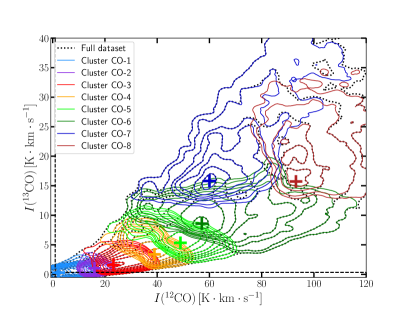
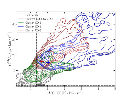
Figure 4 shows the 1D PDF computed for the full dataset and for each individual cluster. The full dataset PDF is clearly multi-peaked with a main peak at low intensities (), two other peaks around 37 and 60 separated by a plateau, and several minor peaks, one of them corresponding to very bright around 90. In contrast, the 1D PDF of and (not shown here) are mostly mono-modal (only one clear peak). A good correspondence between the maxima of the PDF and most of the clusters can be seen. This indicates that plays a major role in the definition of the clusters. Cluster CO-1 corresponds to the highest and narrowest, low-intensity peak, clusters CO-3 and CO-4 constitute the 37 peak, cluster CO-5 contributes to the plateau between the 37 and the 60 peaks, cluster CO-6 and CO-7 corresponds to the 60 peak, and cluster CO-8 corresponds to the clear bump in the high-intensity tail of the PDF (around 90).
However, significant overlap between the clusters can be seen, and two clusters share the 60 peak. Both facts highlight the influence of the other two isotopologues on the clustering. To understand the role of and in the clustering, Fig. 5 shows the 2D PDFs of versus , and versus as contour plots. In each case, the PDF of the full dataset is shown as black dotted contours, while the PDFs of the different clusters are coloured according to the cluster colours presented in Fig. 2. All clusters have clear separations in the versus plane, so that the overlap seen in Fig. 4 is only a projection effect. Clusters CO-1 to CO-5 clearly follow the ridgeline (the line connecting the cluster maxima, similar to the ridgeline of a mountain ridge connecting the summits) of the 2D PDF . The maxima to which they are associated are small bumps along this ridge. The separations of the basins of attraction of each of these maxima thus lie roughly orthogonally to the direction of this ridge. This is probably why the shape of CO-5 cluster looks like an anti-correlation. Clusters CO-2 to CO-5 are associated to relatively small fluctuations of the PDF along the ridge line. While statistically significant, these fluctuations might be too weak to be each attributed a physical meaning: these four clusters might thus represent a single physical category. In the versus space, the PDFs of clusters CO-1 to CO-5 are nearly indistinguishable because they lie below the detection limit. We thus grouped them into a single PDF (grey contours) for better readability.
While clusters CO-6 and CO-7 are undistinguishable on the 1D PDF, they are clearly separated by their 13CO intensities (cluster CO-7 having ). Cluster CO-8 is distinguished both by its high intensity and by higher / ratios at similar intensity than lines of sight belonging to cluster CO-7. Clusters CO-7 and CO-8 thus correspond to a separation of the versus ridge line into two distinct ones at high intensities. Cluster CO-6 is an intermediate cluster that probably lies around the intersection of these two ridge lines. This explains why it is so extended along the axis and narrow along the axis. We discuss these cluster shapes in relation to LTE calculations in Sect. 4.4.
4.3 Relation with volume density and FUV illumination
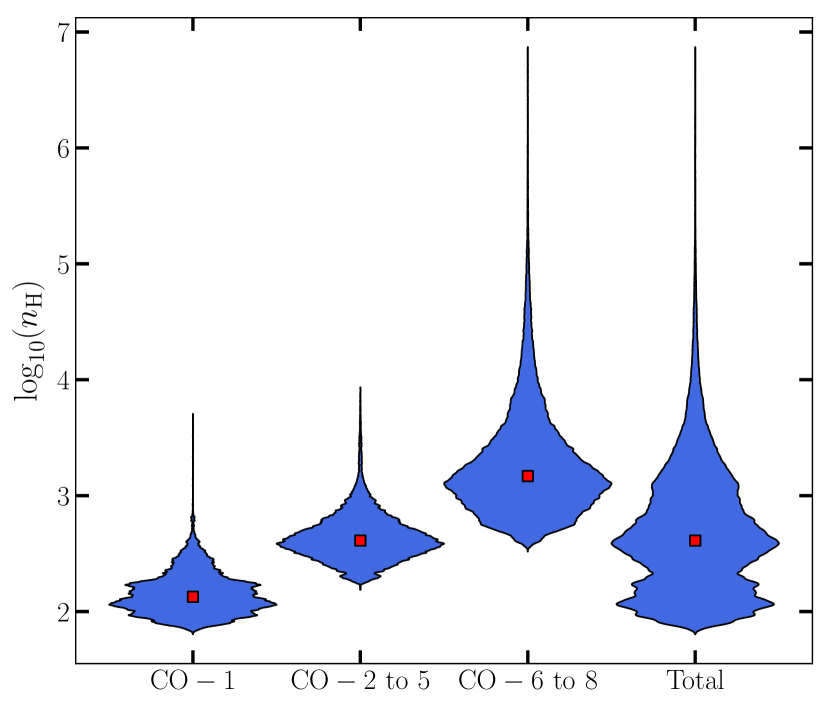
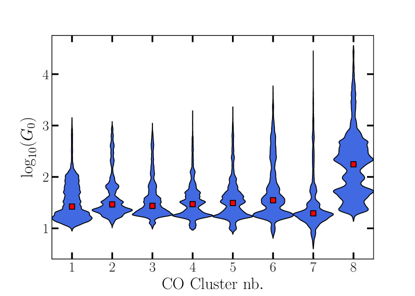
Figure 6 shows how the clusters contribute to the PDF of the approximate volume density (see Section 2.2) in the form of a violin plot: for each group of clusters, the blue profiles show the volume density PDF (normalised to an identical width) and the median values are shown as red squares. We find a close correspondance between our clusters and the three peaks of the density PDF discussed in Sect. 2.2: Cluster CO-1 corresponds to diffuse gas (), the group of clusters CO-2 to CO-5 are associated to translucent gas (), while clusters CO-6, 7, and 8 correspond to denser gas (). The CO clusters thus reveal underlying density regimes.
Figure 7 compares the distributions of the FUV illumination for the different clusters. Clusters CO-1 to CO-6 have similar median values of . Moreover, a higher wing is present for all these clusters. In contrast, cluster CO-7 has a significantly lower value of . This cluster thus tracks gas relatively shielded from the FUV illumination. In addition, the high- wing is negligible for this cluster. Finally, cluster CO-8 has a much larger median value of , and its PDF has two broad components at typical values of and , consistent with the presence of the NGC 2023 and NGC 2024 Hii regions.
In summary, clustering of the CO isotopologues allows us: 1) to distinguish three different regimes of column/volume density (diffuse, translucent, and higher density), and 2) to start distinguishing FUV-illuminated from FUV-shielded gas; but only for relatively dense gas.
4.4 Interpretation: nested CO isotopologues and higher []/[] abundance ratios in FUV-illuminated dense gas
We wish to understand the physical and chemical processes that determine the variations in line intensities detected by the clustering method. We thus make the simplest possible radiative transfer model that will allow us to match the observed line intensities and ratios of the CO isotopologue lines.We then interpret the astrophysical information uncovered by the clustering of the CO isotopologues.
4.4.1 Modeling principles
The typical density over the studied field of view is , and the density of at least 25% of the field (Pety et al. 2017) is larger than (the typical critical density of CO ). We thus chose to use LTE models, as we are mainly interested by the denser parts of the field of view. The clustering analysis taught us that the CO isotopologue intensities trace different ranges of hydrogen column density, and consequently of approximate volume density (See Sect. 2.2). We have thus chosen to model intensity curves for several fixed values of the CO isotopologue column densities, varying the kinetic temperature.
Figure 3 indicates that the structure of the dense inner parts of the cloud is well delineated by the (1–0) emission, still visible in the (1–0) emission, and mostly hidden in the (1–0) emission. The usual interpretation is that the line is so optically thick that the outer, less dense layers along the line of sight can already produce a saturated emission. This means that the and (1–0) lines would be sensitive to denser, cooler gas more deeply embedded along the line of sight while the (1–0) line would to first order be mostly sensitive to the foreground, more FUV-illuminated and thus warmer gas. We thus propose to use two different values for the excitation temperature: a high value for and a lower value for and . This in turn implies that the model column density will be a lower limit to the total CO column density as it only represents the warm gas.
The detailed parametrisation of our modelling is described in Appendix D.
4.4.2 Observations and modeled curves
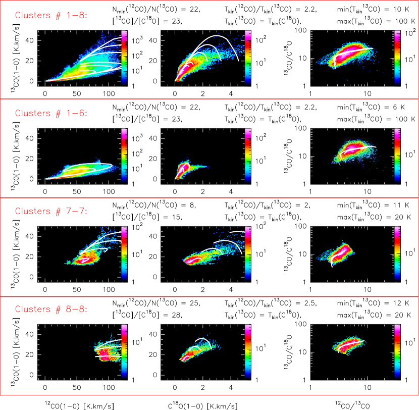
Figure 8 shows the modeled curves over the joint histograms of the versus emission (left column), of the versus emission (middle column), and of the / versus / line ratios (right column). The ratio versus ratio histograms allow us to check how the models take care of the co-variations of the three studied CO lines.
The first row presents the observations for the full field of view, while the next three rows present the observations for different sets of CO clusters (from 1 to 6, the 7th one, and the 8th one, respectively). The sets of input parameters described above each row were chosen to deliver the best visual match between the modelled curves and the three associated histograms.
In all cases, only the lines of sight where the isotopologue lines considered have intensities above are used to compute the histogram. For each opacity (i.e. along each white curve), the and excitation temperature increases clockwise and counter-clockwise for the versus , and versus histograms, respectively. On the ratio versus ratio histograms (right column), the and excitation temperature increases from left to right.
On the line versus line histograms (left and middle columns), the higher the opacity, the more opened the corresponding model curve. In contrast, the dependency on the column density is reduced in the ratio versus ratio histograms, as indicated by the fact that all curves for different opacities almost overlap. This is linked to the fact the line intensity is proportional to the column density to lowest order. And therefore, line ratios remove this trend.
4.4.3 Global results
The first row of Fig. 8 shows the best visual match between observations and models for the full field of view. The FWHM of the lines (2) is the median value measured over the field of view on the 10.5 main component of the and (1–0) lines. The line emission of the modelled curves is integrated over 3 as in the observations.
The range of (1–0) opacities runs from optically thin lines (minimum: 0.03) to moderately saturated lines (maximum: 2.5). The (1–0) line is always optically thin as expected from the fact that (1–0) shows an excellent correlation with the visual extinction (Pety et al. 2017). The (1–0) line is almost always optically thick.
Kinetic temperatures of up to are required to explain the low intensity part of the versus histogram. The abundance ratio is larger than the expected elemental ratio value of (Wilson & Rood 1994). Both inferences can be explained by the significant FUV illumination in the observed field of view, with contributions from external and embedded Hii regions. The joint histogram of versus intensities, especially the range of intensities at a given intensity, can only be explained if and have different kinetic temperatures. In contrast, the observation space can be understood with similar kinetic temperatures of the gas that emits the and (1–0) lines.
4.4.4 Results per CO clusters
In order to better understand how the CO clustering can distinguish different regimes of density and FUV illuminations, we now discuss the input parameters that deliver the best visual match between the modelled curves and the three histograms for three different subsets of the CO clusters.
Starting with the histograms computed for clusters CO-1 to CO-6, shown on the second rows, we obtain the same set of parameters as for the entire field of view (first row). There are only two exceptions. First, we need relatively low opacities (from 0.03 to 0.5), confirming that we deal with low-opacity lines of sight. The horizontal edge between clusters CO-6 and CO-7/8 in the versus histogram closely follows a constant column density curve, confirming that it separates two column density regimes (the cut corresponds to a opacity of ). Second, the minimum kinetic temperature is slightly lower than for the global fit as we are less constrained by the lower edge of the versus histogram. It is unclear whether this fact is significant.
The third and fourth rows show our best matches for clusters CO-7 and CO-8, respectively. In both cases, only the high opacity (0.65 to 2.5) curves are displayed. This confirms that we are in the high-column-density regime. In both cases, we need to restrict the kinetic temperature range from 11-12 to 20. The other parameters differentiate the two clusters. First, the / kinetic temperature ratio is higher in cluster CO-8 than in cluster CO-7. This confirms the idea that the outer layers of the CO-8 cluster are more exposed to the FUV illumination than those of the CO-7 cluster. Finally, the abundance ratio is much closer to the expected elemental abundance ratios for cluster CO-7 than for cluster CO-8. This is consistent with the idea that most of the gas in cluster CO-7 is well shielded, in complete contrast with the gas in cluster CO-8, as discussed in the following section.
4.4.5 Discussion
In all our models, we need to distinguish the kinetic temperature of the gas that emits the (1–0) line on the one hand, and the and (1–0) lines on the other. The effect is the most pronounced in cluster CO-8 that is highly FUV illuminated and then in clusters CO-1 to CO-6 that contain diffuse and translucent gas. This implies that the and / emissions have different spatial extents along the line of sight (as emission quickly saturates and thus only traces a limited surface layer). It is thus impossible to use the flux ratio of these lines to try to infer the []/[] and []/[] abundance ratios.
In the high column/volume density clusters, 12CO is very optically thick (the saturation of the 12CO versus relation is noticeable starting from as shown by Pety et al. 2017), and the variations of integrated intensities are largely caused by variations in the CO excitation temperature, which is close to the gas kinetic temperature. Cluster CO-8 shows significantly higher 12CO intensities () than clusters CO-6 and CO-7 () and thus traces a warmer dense gas regime. This is consistent with its location around the NGC 2024 and NGC 2023 star forming regions.
Cluster CO-8 is also distinguished from cluster CO-7 by higher 13CO/C18O intensity ratios: the median ratio is in cluster CO-8, while it is in cluster CO-7. This difference is a sign of FUV illumination as the 13CO abundance in PDRs is tightly coupled to 12CO by the isotopic fractionation reaction (Langer et al. 1984)
| (5) |
which, at the gas temperatures of PDRs, does not favour any enrichment, but ensures a strong coupling between the abundances of and . In contrast, C18O in FUV-illuminated regions is formed separately from pure carbon chemistry followed by reactions of small hydrocarbons such as CH, CH2 or C2H with 18O. As a result, 13CO indirectly benefits from 12CO self-shielding while is easily dissociated. This might explain the large abundance ratio compared to the value expected from elemental abundances.
Clusters CO-7 and CO-8 thus highlight a separation of the global intensity PDF into two different tails at high column density that correspond to warm illuminated dense regions around massive star forming regions (cluster CO-8) and shielded dense gas (cluster CO-7).
5 Adding HCO+ and CN to get a better clustering of high-density and high-FUV-illumination regimes
Clustering ability is limited by the information contained in the tracers input to the algorithm. Our first application of the Meanshift clustering algorithm to the CO isotopologues proved its ability to reveal several distinct density regimes. It also hinted at a first distinction of FUV illumination regimes. However, using only the three CO isotopologues is insufficient to clearly distinguish FUV illumination effects. We thus now include in the clustering analysis the HCO+ and CN () maps together with the three CO isotopologues maps. Indeed, Pety et al. (2017) and Gratier et al. (2017) have shown that HCO+ and CN were sensitive to FUV illumination. We chose CN rather than small hydrocarbons (C2H or c-C3H2) as the latter are detected at a lower signal-to-noise ratio, making the clustering noisier. For simplicity, we only used the brightest hyperfine component of the CN (1–0) transition. In addition, these two lines have significantly higher critical densities ( for HCO+ and for CN).
We used in this case the adaptive bandwidth method with 425 neighbours. This number is a compromise between eliminating artificial clusters coming from sampling fluctuations of the PDF and retaining sufficiently fine cluster subdivisions to find the interesting physical distinctions.
5.1 Resulting spatial distribution
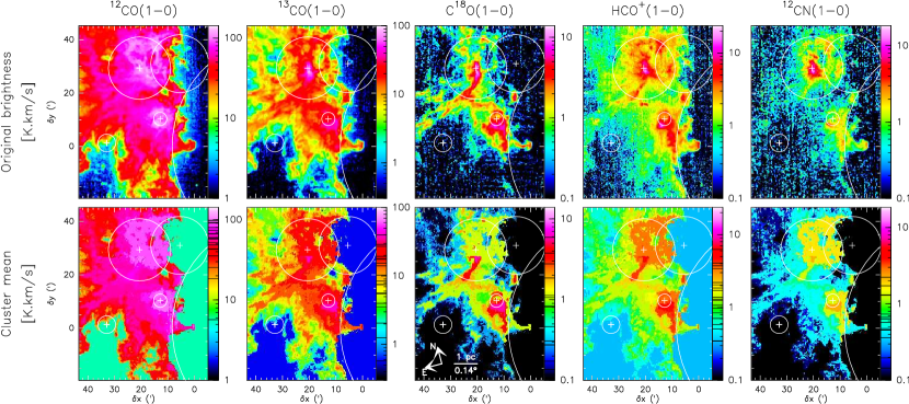
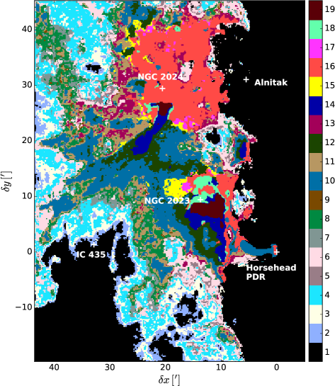
Figure 9 compares the clusters obtained based on the CO isotopologues alone with the clusters obtained by adding CN and HCO+. Several striking facts are visible. First, the CO clustering brought 8 clusters while the new clustering identifies 19 clusters. The increase in number of clusters is related to the finer physics we wish to reveal through the increase of the dimension of the intensity space from 3 to 5 lines, at a constant number of pixels. We name the new clusters FUV-1 to FUV-19. For convenience they have been numbered by order of increasing mean 12CO intensity.
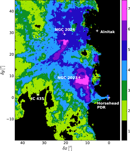
Second, the spatial edges of the FUV clusters that appear from the north-eastern to the south-western corners appear noisier. Indeed, mostly translucent gas is present in these regions, implying that CN and HCO+ are barely detected there. Third, a clear East-West asymmetry is now seen in the distributions of the clusters. Some clusters, such as FUV-2, 3, 4, 7, 8 or 11, appear mostly on regions less exposed to FUV illumination, while cluster FUV-16 is clearly associated with the NGC 2024, NGC 2023, and IC 434 Hii regions. In the previous clustering, cluster CO-8 does not tag the PDRs associated with IC 434 (the Horsehead PDR, for instance). The western edges of the CO-3 to CO-5 clusters are mostly merged now in the cluster FUV-1 that mainly contains diffuse gas. For instance, the envelope of the Horsehead nebula has been merged into FUV-1, only leaving the less familiar silhouette of the denser parts of the Horsehead visible.
Figure 10 compares the spatial distributions of the original line intensities with those of the line intensities averaged per cluster. Comparing with Fig. 3, we see that the FUV clustering reproduces the (1–0) faint intensity regimes less well, but it much better samples the (1–0) high intensity regime and the and median intensity regimes (between 10 and , and between 2 and , respectively). The better sampling of the median- to high-intensity regimes of the CO isotopologue (1–0) lines is linked to the detection of several clusters at relatively high HCO+ integrated intensity . This is particularly clear on the and HCO+ compressed maps that emphasise dense regions extending south of NGC 2024 and surrounding NGC 2023. In contrast, the high-CN-integrated-intensity end is not well sampled by the new clustering.
In summary, this clustering seems to provide most of the FUV illumination contrast between East and West. On the one hand, the FUV clustering thus provides a better data compression in the inner dense parts and in the FUV-illuminated regions; on the other, the shapes of the Horsehead and of the western illuminated edge are less well reproduced.
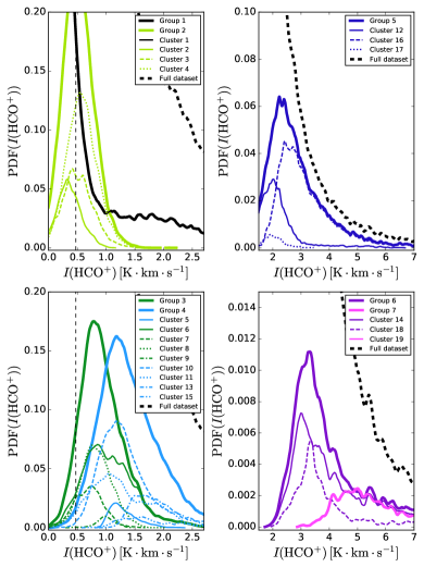
While the 19 clusters are statistically significant, interpreting all of them is difficult. Indeed, clusters with extreme behaviour have relatively clear physico-chemical interpretations but they are separated in the line space by clusters with intermediate properties that reflect subtler, second-order distinctions. The major physical distinctions brought forward by this clustering are thus best discussed in terms of groups of clusters. Moreover, we wish to understand the first-order roles of the HCO+ and CN (1–0) lines in the classification. We thus group the clusters in two ways. We group together clusters with similar most probable intensities of HCO+ or CN respectively, ordered by increasing values. Our goal is to keep the minimum number of groups needed to visualise the physico-chemical regimes first brought forward by each line.
5.2 HCO+-based grouping and high-density regimes
We first constitute groups based on the HCO+ intensities in each cluster following the numerical recipe explained in the previous section.
5.2.1 One-dimensional PDFs and spatial distribution
The left panels of Fig. 11 show the HCO+ PDF of each individual cluster, and the way we grouped them: the clusters whose most probable values (1D-PDF peaks) gather at similar integrated intensities are grouped. We end up with seven groups, named HCO+-1 to HCO+-7, whose mean integrated intensities regularly increase from 0.3 to 6.3. Cluster FUV-1 alone constitutes group HCO+-1 as it mostly traces diffuse gas surrounding the molecular cloud. We nevertheless note that it has a wing between 1 and 3 that corresponds, for instance, to the Horsehead envelope. Group HCO+-2 contains clusters FUV-2, 3 and 4, Group HCO+-3 clusters FUV-6, 7, 8 and 9, group HCO+-4 clusters FUV-5, 10, 11, 13 and 15, group HCO+-5 clusters FUV-12, 16 and 17, group HCO+-6 clusters FUV-14 and 18, and finally, group HCO+-7 contains only cluster FUV-19. The characteristic intensity values (median, mean, standard deviation) of the lines in each group are listed in Table C.
The spatial distribution of these groups is displayed as the right panel of Fig. 11. We see that the resulting groups have a faint mean HCO+ intensity in the outer part of the cloud and that this intensity increases towards the densest parts. In comparison to the CO clustering, the CO-6 to CO-8 bright clusters are now distributed over groups HCO+-3 to HCO+-7, and clusters CO-1 to CO-5 (faint CO intensity) are distributed over the groups HCO+-1 and HCO+-2. This suggests that the HCO+ (1–0) line is better at discriminating higher-density regimes than the CO (1–0) lines, even though about half of the HCO+ flux over the observed field of view is coming from diffuse and translucent regions (Pety et al. 2017). Finally, the boundaries of some groups are close to the CO clustering results, indicating that CO isotopologues still play an important role in defining some of the groups. For instance, the boundary between the HCO+-4 and HCO+-5 groups is similar to the boundary between clusters CO-7/8 and CO-6.
5.2.2 Two-dimensional PDFs
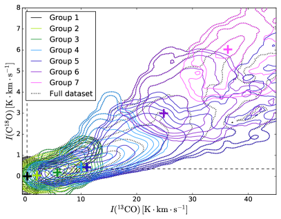
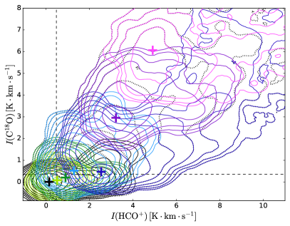
To further understand the relative roles of the CO isotopologues and HCO+, we show in Fig. 12 the 2D-PDFs of 13CO versus C18O (left) and HCO+ versus C18O (right), which we found to be the most informative among the possible pairs of lines. The first striking impression is that the groups overlap considerably in both 2D PDFs. However, some groups clearly separate in one of the 2D PDFs but not in the other. For instance, while groups HCO+-4 and 6 strongly overlap in the (HCO+ vs. C18O) PDF, they are cleanly separated in the (13CO vs. C18O) PDF. Finding the right 2D projection to reveal cluster separations quickly becomes impossible. Moreover, this 2D projection might not even exist when the clusters are not linearly separable; for example, when one cluster is completely surrounded by another one. We have to rely on the Meanshift algorithm to reveal information about the morphology of the complete PDFs (maxima and their associated basins of attraction) that we cannot otherwise directly visualise.
The groups form a sequence that mostly follows a single trend with increasing line intensities. This is better visualised when trying to connect the crosses that represent the group mean intensities. Group HCO+-5 only partially follows this trend: a part of it (actually mostly cluster FUV-16) is overluminous in HCO+ at constant intensity. This is linked to the sensitivity of the HCO+ (1–0) line to the FUV illumination (cf. the following section).
5.2.3 Link with volume density and FUV illumination
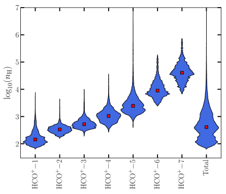
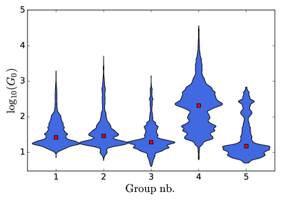
As shown in Gratier et al. (2017), the main underlying parameter contributing to intensity variations across our maps is the gas column density. The single trend highlighted here could thus to first order be associated with column density variations and thus approximate volume density variations as discussed in Section 2.2. Figure 13 shows the PDF and median value of the volume density in each group (violin plots). We indeed see that the HCO+-groups correspond to increasing ranges of volume densities. On the one hand, the first five HCO+-groups contribute to the three main peaks of the approximate volume density PDF: the HCO+-1 group corresponds to the diffuse gas peak, the HCO+-2 and 3 groups dominate the translucent gas peak, and the HCO+-4 and 5 groups contribute to the denser gas peak. On the other hand, groups HCO+-6 and 7 are located in the high-density tails.
While part of the distinction is linked to the underlying existence of the three density regimes, the distinction between groups HCO+-6 and 7 hints at the existence of higher-density regimes. Their rarity makes them only barely noticeable as bumps in the density PDF. This distinction is probably the result of an excitation effect. Indeed, their typical volume densities (probably underestimated as they are averaged along the line of sight) are , and , respectively. These values approach the critical density of HCO+ for collisional excitation with H2 (). We thus probably experience a transition from a weak excitation regime (Liszt & Pety 2016) towards a regime closer to the usual thermalised excitation.
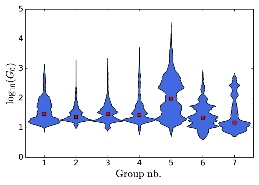
Figure 14 shows the PDF and median value of the FUV illumination for each group. In contrast to the density, no clear separation of the groups in terms of FUV illumination is visible, except for the fact that HCO+-5 has a much broader distribution than the other groups. The HCO+ grouping thus does not cleanly capture distinctions only related to FUV illumination, even though the complex behaviour of HCO+-5 in the 2D PDFs of the line intensities is likely related to the presence of a mixture of FUV illumination (varying by more than one order of magnitude) in this group. This is not a property of the initial 19 clusters but of the grouping, as is shown in the following Section.
5.3 CN-based grouping and FUV illumination regimes
We now present the second grouping of the clusters, based on their CN intensities.
5.3.1 One-dimensional PDFs and spatial distribution
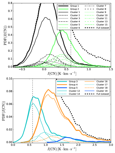
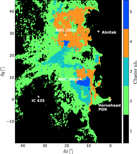
The left panels of Fig. 15 show how the CN PDF of the individual clusters contributes to the PDF of their group. After sorting them by increasing CN mean intensity, we merged the first six clusters into group CN-1 (clusters FUV-1, 2, 3, 4, 7, 8) because they correspond to regions where CN is not detected. We then merged the next seven clusters into group CN-2 (clusters FUV-5, 6, 9, 10, 11, 13, 15). The CN line is barely detected in these clusters. Groups CN-3 and CN-4 gather the next three (FUV-12, 14 and 17) and two clusters (FUV-16 and 18), respectively. The last cluster (FUV-19) is significantly brighter in CN. It thus has its own group CN-5. The characteristic intensity values (median, mean, standard deviation) of the lines in each group are listed in Table C.
The most striking distinction revealed by the resulting spatial distribution (see the right panel of Fig. 15) is the separation of the central regions of the cloud between groups CN-3 and CN-4; contrary to the previous cases, this separation does not show a nested pattern. The CN-3 group covers dense regions in the inner parts of the cloud. The CN-4 group appears towards the interfaces between the molecular cloud and the NGC 2024, NGC 2023, and IC 434 Hii regions. This distinction thus seems to separate FUV-shielded dense gas (group CN-3) and FUV-illuminated dense gas (group CN-4). Group CN-5 highlights smaller regions at the interface between groups CN-3 and CN-4. Groups CN-1 and 2 represent outer regions of the cloud.
5.3.2 Two-dimensional PDFs
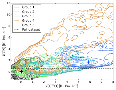
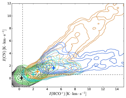
Figure 16 shows the 2D PDFs of CN versus C18O (left panel), and CN versus HCO+ (right panel); it compares the full dataset PDF (dashed line) with the contributions of our five groups (solid lines). Two distinct trends in the tail of the PDF are obvious on the 2D PDF of CN versus HCO+: a low CN/HCO+ ratio corresponding to group CN-5, and a high CN/HCO+ ratio corresponding to group CN-4. The other groups lie in a low-intensity region where the two trends are blended.
This dual trend is already seen on the (CN vs. C18O) 2D-PDF: for groups CN-2, CN-3, and CN-5, CN increases very slowly with C18O, in a mostly linear way. In contrast, group CN-4 has higher CN intensities than the other groups, with the CN intensity increasing much faster with the C18O one; although this trend has a larger scatter.
Finally, while there is a large overlap region between groups CN-4 and CN-5 in the PDF of CN versus HCO+, these two groups are clearly separated in the PDF of CN versus C18O. Group CN-4 is thus observationally distinguished by an overly bright CN emission.
5.3.3 Link with FUV illumination (and volume density)
As a species easily detected in diffuse clouds, CN is a good tracer of FUV-illuminated gas (Snow & McCall 2006). We thus interpret the dual trend as a separation between regions where the photo-chemistry is active and regions of dense FUV-shielded molecular gas. The spatial consistency of groups CN-3 with regions of dense FUV-shielded gas and CN-4 with FUV-illuminated gas strengthens this interpretation, all the more so that spatial information is not used in the clustering analysis.
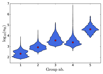
More quantitatively, Fig. 17 shows the approximate volume densities (left panel) and FUV illuminations (right panel) found for the different groups. Groups CN-3 and CN-4 have very similar volume densities (median densities of and , respectively), while the CN-1, CN-2, and CN-5 correspond to distinct ranges of volume densities (respective median densities of , and ). In contrast, the distributions show that group CN-4 clearly has higher FUV illumination (median ) than all other groups (median between 15 and 30), in particular groups CN-3 and CN-5 (median and , respectively). This confirms our interpretation that group CN-4 corresponds to FUV-illuminated (relatively) dense gas.
Groups CN-1 and CN-2 have lower approximate volume densities than groups CN-3 and CN-4. However the distribution of and therefore in groups CN-1 and CN-2 overlaps with that of both groups CN-3 and CN-4. This shows that it is more difficult to separate the influence of the radiation field for low-density regions. This is related to the fact that the envelope of the Horsehead nebula has been merged into group CN-1, leaving only the less familiar silhouette of the denser parts of the Horsehead visible.
The highest-density group (CN-5) is found only in the immediate vicinity of the two star-forming regions NGC 2023 and NGC 2024 and their Hii regions. This might be a signature of compression of the molecular gas by the expansion of the Hii regions: Tremblin et al. (2014) have indeed found this process to cause bimodality in the column density PDF (on spatial scales of a few pc). The gas kinematics in these two regions was in addition found to be dominated by compressive (rather than solenoidal) motions by Orkisz et al. (2017), in contrast to the rest of the field of view.
5.3.4 Interpretation: Enrichment of HCO+ and CN with respect to in FUV-illuminated gas
The PDFs of HCO+ versus C18O and CN versus C18O show a dual regime at high C18O (1–0) intensity (cf. Fig. 12, right panel, and Fig. 16, left panel), with one regime where HCO+ and CN are overluminous relative to . This latter regime is clearly associated with high FUV illumination at high volume density. We here check whether this is the sign of a chemical enrichment of HCO+ and CN in FUV-illuminated regions, using a non-LTE code (RADEX, van der Tak et al. 2007) to estimate the column densities of these species.
The modeling details and the derived column densities are described in Appendix E. For simplicity, we only model the radiative transfer for typical conditions in each group (median gas volume density, median kinetic temperature, and median line integrated intensities). As an estimate of the kinetic temperature, we take a combination of the dust temperature and the 12CO excitation temperature as in the Appendix A of Orkisz et al. (2017): we take the excitation temperature when it is above 60, and the maximum of the dust temperature and excitation temperature otherwise.
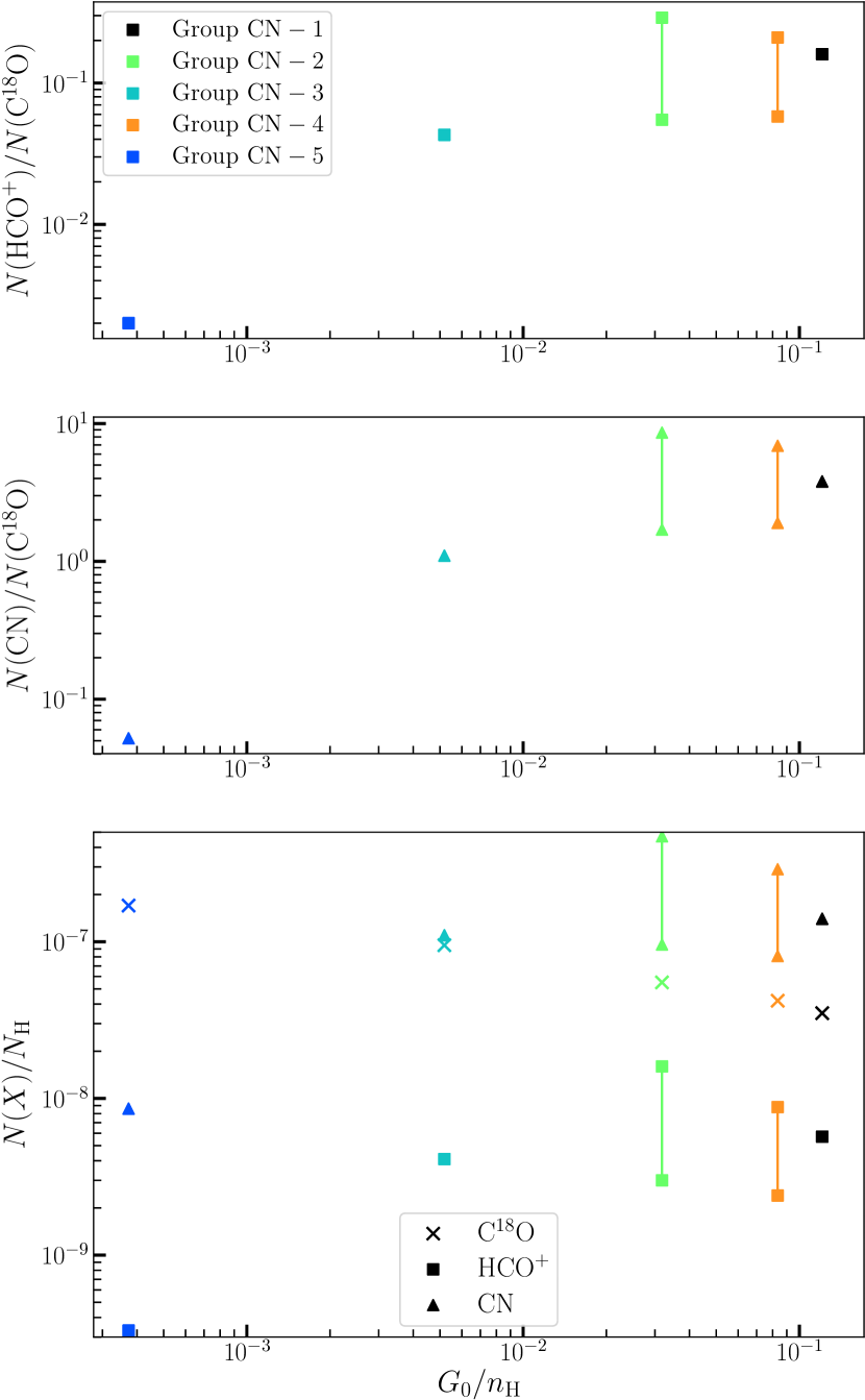
Figure 18 shows the behaviour of the derived abundance ratios [HCO+]/[C18O], and [CN]/[C18O] as a function of the parameter, which is expected to be the dominant controlling parameter of the physics and chemistry in a PDR (Hollenbach & Tielens 1997). An increase by about two orders of magnitude of the HCO+ and CN abundances relative to C18O can be seen when increasing . The abundances relative to seem to reach a constant value at high values in both cases.
Fractional abundances for each of the three species are also computed relative to the total (dust-derived) column density . These abundances are shown in the lower panel of Fig. 18 as a function of . Both the HCO+ and CN abundances steeply increase with with at first (up to ), before saturating at a nearly constant value up to . The abundance smoothly decreases with increasing over the full range of values. This marked difference of chemical behaviour therefore explains the difference in line intensities identified by the MeanShift algorithm. The abundances of CN and HCO+ remain at a high but nearly constant value in strongly or mildly FUV-illuminated regions, while the abundance decreases with increasing FUV illumination. The overbright HCO+ and CN regime found in FUV-illuminated regions is thus caused by a combination of photochemical enrichment in CN and HCO+ and photodissociation of .
6 The Meanshift algorithm, an interesting clustering method: biases and data requirements
We first present why and how clustering and principal component analysis are complementary. We then discuss the effects (noise, sampling, dimensionality) that can alter our results.
6.1 On the complementarity of clustering and principal component analyses
We chose here to use a clustering approach in order to analyse the structure of the multi-dimensional PDF of several line intensities, based on the idea that this structure can reveal interesting insights into the physics and chemistry at play. As soon as we use a dataset with more than two dimensions, visualising the structure of its PDF becomes difficult, and specific methods must be used. Each of these methods is usually focused on highlighting a particular kind of structure, and applying different methods to the same dataset thus provides complementary results.
For instance, clustering provides a complementary approach to Principal Component Analysis (PCA). On the one hand, PCA highlights the non-sphericity of the data by revealing the axes of strong covariance or correlation. However, PCA cannot capture non-linear patterns of co-variations between the intensities. Moreover, PCA highlights variations around a centre of the dataset (usually the mean), which might not be relevant if the data points are gathered in several natural clusters, with different centres (that is, if the PDF is multimodal). On the other hand, clustering algorithms aim at revealing any grouping of the data points in different regions of intensity space, that is, to reveal multimodality in the (multi-dimensional) PDF of the data.
By applying PCA to this dataset, Gratier et al. (2017) showed that column density, volume density, and FUV illumination are some of the underlying parameters controlling the intensity variations. And they listed the tracers that are the most affected by each of these parameters. The clustering analysis we have performed in the present study reveals, in addition, a multimodality of the line intensity PDF with modes related to the density and the FUV illumination. In the case of the CO clustering, the modes of the CO isotopologue PDF are directly related to modes of the column/volume density PDF, thus revealing the existence of distinct density regimes in the Orion B cloud. In our clustering analysis including HCO+ and CN, the transition to a photon-dominated chemistry leads to a separate mode corresponding to dense PDRs. In this case, clustering reveals a transition between two different physical/chemical regimes.
Moreover, both approaches can be used as data compression methods, in order to reduce the volume of data before applying some other very time-consuming data analysis. PCA compresses the dataset by reducing the number of variables characterising each data point, while clustering can be used as a segmentation method, discretising the possible values of each variable. Finally, these two approaches could be combined in future work. One possibility would be to decompose a multi-line PDF into separate components with simpler structure before applying PCA to each of these components. Alternatively, a PCA analysis could be performed first to eliminate irrelevant components of the data (e.g. noise), followed by a clustering analysis restricted to the relevant features deduced by the PCA.
6.2 What is the impact of noise?
The effect of the measurement noise present in our line-intensity maps on the results of the Meanshift algorithm can be understood in two ways: 1) Its effect on the data PDF, used by the Meanshift algorithm to define clusters, and 2) its effect on the attribution of a given pixel to one of the clusters.
Assuming an identical noise rms, , on all datapoints (a good approximation for this dataset, see Pety et al. 2017), the addition of Gaussian noise to the true variables replaces the underlying PDF by an observed PDF that is the convolution of the underlying PDF with a Gaussian of standard deviation . This is equivalent to a Gaussian smoothing of the PDF. This effect will mostly tend to merge some maxima if their separation is too small compared to the smoothing scale (that is, the noise level), rather than creating artificial maxima. The smoothing effect can also slightly shift the position of the extrema. But the existence of the clusters will be unaffected as long as their PDF maxima are well separated compared to the smoothing scale.
Noise also alters the boundaries between the clusters. If the true intensity values of a given pixel place it close enough to a boundary between clusters in the line space (typically closer than the noise level), adding noise can move this pixel across the border, and thus change the cluster to which it belongs. As a result, noise on the line intensities tends to make the spatial boundaries between clusters appear noisy (not forming a regular curve on the map). This effect is more pronounced in regions of the map where intensity gradients are small. In this case, pixels relatively far away from the cluster spatial boundary can still be close to the cluster boundary in the line space and thus be transferred to another cluster. On the contrary, if intensity gradients are steep at the spatial boundary, even pixels located just one or two pixels away from the spatial boundary can be far enough from the cluster boundary in the line space so that noise is unlikely to transfer them to another cluster. This effect is at play when we include CN and HCO+ which have low signal-to-noise ratios on significant fractions of the map. Relatively noisy boundaries can be seen on the eastern side of the cloud while the boundaries on the western edge remain sharp (cf. Fig. 9). The intensity gradients are indeed much steeper on the western side of the cloud than on the eastern side.
6.3 What is the impact of limited sampling (field of view)?
The Meanshift algorithm estimates the PDF gradient in the line space in order to find the PDF maxima, and it needs to estimate this gradient from a finite sample (the observed dataset). There are two different aspects here. First, the observed field of view may be biased towards some values of the parameters that control the physics or the chemistry. Pety et al. (2017) showed that this is the case here, as the studied field of view has a large FUV illumination compared to the Interstellar Standard Radiation Field because it includes several Hii regions. In the ORION-B project, we will increase the observed field of view towards regions of lower FUV illumination to circumvent this limitation. In the meantime, our clustering analysis must be interpreted with this limitation in mind.
Second, the gradient estimate can be affected by sampling noise: a different dataset drawn from the same underlying PDF (corresponding to this specific field of view) would yield slightly different gradient estimates, and thus converge towards slightly different maxima. We chose to use an adaptive bandwidth (so that the kernel always includes the same number of datapoints), rather than a fixed bandwidth (which would give better sampled gradient estimates close to the major PDF peaks than in the tails) to reduce the impact of this effect. This ensures that the sampling noise is similar for all gradient estimations, and it avoids finding sampling-noise-induced artificial maxima in the tail of the PDF. Having at least a few hundred datapoints in the kernel generally ensures that the sampling noise has negligible effect.
However, implicitly increasing the kernel bandwidth in low-density regions of the PDF means a decreased capacity to resolve small-scale features in the PDF. As a result, PDF maxima corresponding to a small number of pixels (compared to the kernel size) might be smoothed out unless these pixels have intensities widely different from all other pixels. This means that our analysis is likely to miss specific physical or chemical regimes if they occur on too small a region of the map. This was the case in our tests where we found that dense cores are difficult to capture as a cluster with the Meanshift algorithm even when including specific dense core chemical tracers such as N2H+.
6.4 Choice of the number of molecular lines included in the analysis
In contrast to our PCA study (Gratier et al. 2017), we limited the clustering analysis to a moderate number of lines (5 at most). This choice was driven by several considerations.
The first reason is practical. As discussed in Sect. 6.2, while including low signal-to-noise-ratio (SNR) line maps may change the total number of clusters, the presence of such low-SNR data always degrades the quality of the cluster boundaries. Well defined clusters with clear interfaces are only obtained in the regions where all lines have high SNR. A consequence of using several lower-brightness lines at relatively constant noise level (our observing case) is therefore a reduction of the usable pixels to the regions where all the lines have high SNR, that is the regions of highest column densities. This requirement of significant SNR for all line maps limits the usefulness of the Meanshift algorithm when applying it to a large set of lines of varying SNR. We thus restricted our study to lines showing extended emission with high SNR on a large fraction of the map.
The second reason is more fundamental. In this paper, we try to understand the physical and chemical processes that regulate the intensities of the lines used in the clustering algorithm. The clustering of the CO isotopologue ground-state line maps, complemented by the HCO+ and CN lines, showed two trends. First, the number of significant clusters increases with the number of lines because we add lines that exhibit different sensitivities to the physical or chemical processes at work. Second, the interpretation of a large number of clusters is difficult because the associated clusters have less data points implying a lower statistical significance of the trends. Moreover, it is difficult to get a good appreciation of the full distribution of the data over which the Meanshift algorithm operates in dimensions larger than two through standard 2D PDFs.
Our experience is thus that it is better to start clustering in low dimension to understand the sensitivity of the different lines to the many underlying physical and chemical processes at play in the ISM. It will then be possible to cluster higher-dimension data to get a finer segmentation that will depend on the underlying properties that need to be emphasised.
7 Conclusions
In this paper, we present a segmentation of the Orion B molecular cloud into regions of similar molecular emission, in order to reveal the different physical and chemical phases constitutive of molecular clouds. We have applied the Meanshift algorithm, a PDF-based (unsupervised) clustering algorithm defining clusters around the maxima of the PDF, to the (high-dimensional) multi-line PDF of our dataset. This is the first application of a clustering analysis based on molecular emission properties only (and not spatial proximity between pixels) to ISM data.
We first applied the clustering analysis to the maps of the three main CO isotopologue lines only. While the clustering did not take the spatial distribution of the CO emission into account, it highlighted a nested pattern from the outer edges to the innermost parts of the Orion B cloud. Comparison with an approximate volume density map showed that the clusters have increasing typical volume densities with significant grouping at densities of 100, 500, . The CO isotopologue maps alone were thus found to be sufficient to reveal the existence of the diffuse, translucent and high-column-density regimes. Simple LTE radiative transfer modelling implies that the gas emitting the (1–0) line is more extended than the gas emitting the / (1–0) lines. It is thus impossible to use the flux ratio of these lines to try to infer the []/[] and []/[] abundance ratios.
In the densest regime, an additional separation of the PDF in two distinct tails was found, which we could associate to FUV-illumination effects. Comparison with LTE radiative transfer models shows that this distinction is related to the presence of a warmer -traced surface layer and higher than usual []/[] ratios, which can both be explained by the increased FUV illumination caused by the nearby Hii regions. It however proved insufficient to get a satisfactory separation of the FUV illuminated regions.
We thus added two FUV-sensitive tracers (the lines of HCO+ and CN) to the CO isotopologues, and performed a second clustering analysis. This analysis revealed a similar separation into increasing density regimes, but captured finer distinctions at higher density ( and ) due to the high critical density of the added tracers. Pety et al. (2017) have however shown that about half of the HCO+ flux over the observed field of view is coming from diffuse and translucent regions, implying that the use of the HCO+ line intensity as a tracer of high density gas in unresolved GMC observations is questionable.
Moreover, the clustering also revealed the existence of another clear separation of the data at high column density. On the one hand, part of the data presents a CN and HCO+ (1–0) emission that is overly bright with respect to the (1–0). This data also shows a high CN/HCO+ intensity ratio. The associated lines of sight form the dense PDR regions around the star forming regions NGC 2023 and NGC 2024, and on the Orion B western edge illuminated by Ori (including the Horsehead PDR). On the other hand, other high-column-density lines of sight have low CN/, HCO+/, and CN/HCO+ intensity ratios. These lines of sight correspond to the FUV-shielded, dense regions in the inner parts of Orion B. Non-LTE models show that this distinction is related to a clear increase of the [HCO+]/[] and [CN]/[] abundance ratios with .
Our clustering analysis based on the (1–0) lines of the CO isotopologues, HCO+ and CN, thus managed to both capture finer density categories in the densest regions, and to reveal the existence of two distinct chemical phases (characterised by different abundance ratios) corresponding to FUV-induced photochemistry and shielded-gas chemistry. This exposes the wealth of physical and chemical information that can be inferred from molecular tracers when powerful statistical methods (as the Meanshift algorithm) are applied to large amounts of data. One of the next steps in the ORION-B project is to stack the spectra inside each of the clusters found here, to better characterise the molecular content of each regime using the whole information available in the 3 mm band.
Acknowledgements.
The authors thank the referee for his constructive comments, useful suggestions, and his very fast refereeing. EB post-doctoral position during this work was funded by the ERC grant ERC-2013-Syg-610256-NANOCOSMOS. This work was in part supported by the Programme National “Physique et Chimie du Milieu Interstellaire” (PCMI) of CNRS/INSU with INC/INP, and co-funded by CEA and CNES. We thank the CIAS for its hospitality during the three workshops devoted to this project. JRG thanks the Spanish MINECO for funding support through grant AYA2012-32032. NRAO is operated by Associated Universities Inc. under contract with the National Science Foundation. This paper is based on observations carried out at the IRAM-30 m single-dish telescope. IRAM is supported by INSU/CNRS (France), MPG (Germany) and IGN (Spain). This research also used data from the Herschel Gould Belt survey (HGBS) project (http://gouldbelt-herschel.cea.fr). The HGBS is a Herschel Key Programme jointly carried out by SPIRE Specialist Astronomy Group 3 (SAG 3), scientists of several institutes in the PACS Consortium (CEA Saclay, INAF-IFSI Rome and INAF-Arcetri, KU Leuven, MPIA Heidelberg), and scientists of the Herschel Science Center (HSC).References
- Allison & Dalgarno (1971) Allison, A. C. & Dalgarno, A. 1971, A&A, 13, 331
- André et al. (2010) André, P., Men’shchikov, A., Bontemps, S., et al. 2010, A&A, 518, L102
- Bishop (2006) Bishop, C. 2006, Pattern Recognition and Machine Learning (Springer-Verlag New York)
- Black & van Dishoeck (1991) Black, J. H. & van Dishoeck, E. F. 1991, ApJ, 369, L9
- Carpenter (2000) Carpenter, J. M. 2000, AJ, 120, 3139
- Colombo et al. (2015) Colombo, D., Rosolowsky, E., Ginsburg, A., Duarte-Cabral, A., & Hughes, A. 2015, MNRAS, 454, 2067
- Comaniciu & Meer (2002) Comaniciu, D. & Meer, P. 2002, IEEE Transactions on Pattern Analysis and Machine Intelligence, 24, 603
- Comaniciu et al. (2001) Comaniciu, D., Ramesh, V., & Meer, P. 2001, in in Proc. 8th Intl. Conf. on Computer Vision, 438–445
- Epanechnikov (1969) Epanechnikov, V. A. 1969, Theory of Probability & Its Applications, 14, 153
- Ester et al. (1996) Ester, M., Kriegel, H.-P., Sander, J., & Xu, X. 1996, in Knowledge Discovery and Data Mining Conference (AAAI Press), 226–231
- Faure & Tennyson (2001) Faure, A. & Tennyson, J. 2001, MNRAS, 325, 443
- Feigelson & Babu (2012) Feigelson, E. D. & Babu, G. J. 2012, Modern Statistical Methods for Astronomy
- Flower (1999) Flower, D. R. 1999, MNRAS, 305, 651
- Fuente et al. (2008) Fuente, A., García-Burillo, S., Usero, A., et al. 2008, A&A, 492, 675
- Georgescu et al. (2003) Georgescu, B., Shimshoni, I., & Meer, P. 2003, in Computer Vision, 2003. Proceedings. Ninth IEEE International Conference on, 456–463 vol.1
- Goldsmith & Kauffmann (2017) Goldsmith, P. F. & Kauffmann, J. 2017, ApJ, 841, 25
- Gratier et al. (2017) Gratier, P., Bron, E., Gerin, M., et al. 2017, A&A, 599, A100
- Habing (1968) Habing, H. J. 1968, Bull. Astron. Inst. Netherlands, 19, 421
- Hollenbach et al. (1991) Hollenbach, D. J., Takahashi, T., & Tielens, A. G. G. M. 1991, ApJ, 377, 192
- Hollenbach & Tielens (1997) Hollenbach, D. J. & Tielens, A. G. G. M. 1997, ARA&A, 35, 179
- Inglada et al. (2017) Inglada, J., Vincent, A., Arias, M., et al. 2017, Remote Sensing, 9, 95
- Jolliffe (2002) Jolliffe, I. 2002, Principal Component Analysis, Springer Series in Statistics (Springer-Verlag New York)
- Kirk et al. (2016) Kirk, H., Di Francesco, J., Johnstone, D., et al. 2016, ApJ, 817, 167
- Krčo & Goldsmith (2016) Krčo, M. & Goldsmith, P. F. 2016, ApJ, 822, 10
- Lada (1992) Lada, E. A. 1992, ApJ, 393, L25
- Langer et al. (1984) Langer, W. D., Graedel, T. E., Frerking, M. A., & Armentrout, P. B. 1984, ApJ, 277, 581
- Lique et al. (2010) Lique, F., Spielfiedel, A., Feautrier, N., et al. 2010, J. Chem. Phys., 132, 024303
- Liszt (2012) Liszt, H. S. 2012, A&A, 538, A27
- Liszt & Pety (2016) Liszt, H. S. & Pety, J. 2016, ApJ, 823, 124
- Lombardi et al. (2014) Lombardi, M., Bouy, H., Alves, J., & Lada, C. J. 2014, A&A, 566, A45
- Martin-Zaïdi et al. (2008) Martin-Zaïdi, C., Deleuil, M., Le Bourlot, J., et al. 2008, A&A, 484, 225
- McCauley et al. (2011) McCauley, P. I., Mangum, J. G., & Wootten, A. 2011, ApJ, 742, 58
- Megeath et al. (2016) Megeath, S. T., Gutermuth, R., Muzerolle, J., et al. 2016, AJ, 151, 5
- Menten et al. (2007) Menten, K. M., Reid, M. J., Forbrich, J., & Brunthaler, A. 2007, A&A, 474, 515
- Orkisz et al. (2017) Orkisz, J. H., Pety, J., Gerin, M., et al. 2017, A&A, 599, A99
- Parzen (1962) Parzen, E. 1962, Ann. Math. Statist., 33, 1065
- Pedregosa et al. (2011) Pedregosa, F., Varoquaux, G., Gramfort, A., et al. 2011, Journal of Machine Learning Research, 12, 2825
- Pety et al. (2017) Pety, J., Guzmán, V. V., Orkisz, J. H., et al. 2017, A&A, 599, A98
- Planck Collaboration et al. (2011) Planck Collaboration, Ade, P. A. R., Aghanim, N., et al. 2011, A&A, 536, A1
- Rosenblatt (1956) Rosenblatt, M. 1956, Ann. Math. Statist., 27, 832
- Rosolowsky & Leroy (2006) Rosolowsky, E. & Leroy, A. 2006, PASP, 118, 590
- Schlafly et al. (2014) Schlafly, E. F., Green, G., Finkbeiner, D. P., et al. 2014, ApJ, 786, 29
- Schneider et al. (2013) Schneider, N., André, P., Könyves, V., et al. 2013, ApJ, 766, L17
- Shimajiri et al. (2017) Shimajiri, Y., André, P., Braine, J., et al. 2017, ArXiv e-prints
- Snow & McCall (2006) Snow, T. P. & McCall, B. J. 2006, ARA&A, 44, 367
- Sobolev (1960) Sobolev, V. V. 1960, Sov. Ast., 4, 1
- Stutzki & Guesten (1990) Stutzki, J. & Guesten, R. 1990, ApJ, 356, 513
- Tremblin et al. (2014) Tremblin, P., Schneider, N., Minier, V., et al. 2014, A&A, 564, A106
- van der Tak et al. (2007) van der Tak, F. F. S., Black, J. H., Schöier, F. L., Jansen, D. J., & van Dishoeck, E. F. 2007, A&A, 468, 627
- Ward-Thompson et al. (2006) Ward-Thompson, D., Nutter, D., Bontemps, S., Whitworth, A., & Attwood, R. 2006, MNRAS, 369, 1201
- Williams et al. (1994) Williams, J. P., de Geus, E. J., & Blitz, L. 1994, ApJ, 428, 693
- Wilson & Rood (1994) Wilson, T. L. & Rood, R. 1994, ARA&A, 32, 191
- Yang et al. (2010) Yang, B., Stancil, P. C., Balakrishnan, N., & Forrey, R. C. 2010, ApJ, 718, 1062
Appendix A Column density and approximate volume density

In this Section, we explore whether the assumptions of isotropy and of a nested distribution of volume density (density smoothly increasing from the outer regions to the inner parts of the cloud) can be used to derive an approximate volume density from the spatial distribution of the column density. After a discussion of the spatial and statistical distributions of the column density, we use the above assumptions to derive an approximate volume density. We then compare the derived values to previously published measures of the density in this field of view to understand the limits of the method and to estimate its accuracy.
Figure 19 shows the spatial (panel a) and statistical (panel b) distributions of the gas column density deduced from the dust continuum emission (see Sect. 2.2). The targeted region exhibits a large range of column densities. There is slightly more than a factor of 100 between the minimum and maximum values. A hypothesis of nearly constant gas volume density would imply that the high-column-density regions should be about one hundred times deeper than the low-column-density ones, which would require an unrealistic cloud geometry. Moreover, the spatial distribution of the column density shows a nested pattern. Indeed the highest-column-density contours are surrounded by the smaller-column-density ones. This is also easily seen on the column density PDF (Fig. 1), which shows a faint tail at high column density. Higher-column-density regions must thus be less extended along the line of sight (according to our isotropy hypothesis), and as a consequence be associated with higher volume densities, at least in the statistical sense.
Assuming the simplest possible hypotheses about the spatial distribution of volume density, that is the hypothesis of no privileged direction and nested increasing volume density, we estimate the typical lengthscale of regions with a given column density value as the square root of the projected surface area where . Pixels with are then given the volume density . This procedure is illustrated in the last three panels of Fig. 19. This reasoning assumes a one to one correspondence between a column density and the approximate volume density. We only expect this relationship to hold in a statistical sense: it may not be valid pixel by pixel but we expect it to correctly represent the range of volume densities at a given column density.
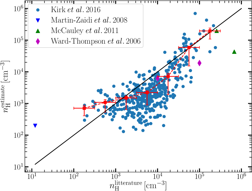
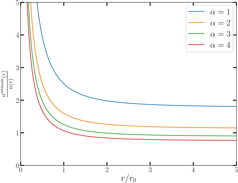
In order to estimate the accuracy of this estimate, we gathered volume density estimations from the literature at positions within our field of view, and derived from a variety of different methods. From the catalogue of cores of Kirk et al. (2016) (SCUBA dust emission observations), we derived core masses from their Eq. 3 (using the background-substracted fluxes), and we complemented the mass value with their measured size to yield volume densities. We completed this sample with a few density estimates at particular positions. The volume density of the diffuse foreground gas of HD 38087 was derived by Martin-Zaïdi et al. (2008) from H2 UV absorption lines through the use of PDR models. The volume densities for two positions in NGC2024 was inferred from H2CO emission lines (McCauley et al. 2011). And the volume densities in the B33-SMM1 and B33-SMM2 cores in the Horsehead were derived from dust emission observations (Ward-Thompson et al. 2006). Figure 21 shows our volume density estimates compared to the ones from the literature. In addition, the red points and their error bars show the average of our density estimate in log-spaced bins of the literature density values.
On average, our density estimate is within a factor of 3 of the densities from the literature, with a typical scatter of one order of magnitude. For the diffuse medium data point of Martin-Zaïdi et al. (2008), we find a density times larger. This is consistent with the typical scatter, but could also come from a bias of our estimate at low densities, as our lengthscale estimate is limited to the size of our field of view while diffuse medium might span larger scales. We note that our estimate is however qualitatively correct by predicting a diffuse-medium-like density at this position.
As an additional check, we consider a simple analytical example: a spherically symmetrical cloud whose volume density profile is
| (6) |
(used for instance in Krčo & Goldsmith 2016). This corresponds to an observed column density profile
| (7) |
Our simple estimate of the volume density would yield at a distance from the cloud centre
| (8) |
The ratio of the two values,
| (9) |
is shown on Fig. 21 for different values of . Our estimation ranges from 0.8 to 2.5 times the true density value for all estimation scales larger than the typical scale and it diverges when the estimation scale is much smaller than . This comes from the fact that the surface estimate describing the scale of the inner region goes to zero close to the centre. However, the spatial resolution of our data (60 mpc) avoids the regime . Indeed, our comparison to literature values does not show any dramatic overestimation for the high-column-density pixels.
In conclusion, the method proposed here provides a reasonable estimate in a statistical sense with a bias of a factor 3 at most and a typical scatter of one order of magnitude. It can thus be trusted for order-of-magnitude comparisons. Moreover, this estimation of the volume density map is completely independent from the clustering analysis presented in this paper, and is only used to help in the interpretation of the clustering analysis.
Appendix B Impact of the number of neighbours on the number of clusters
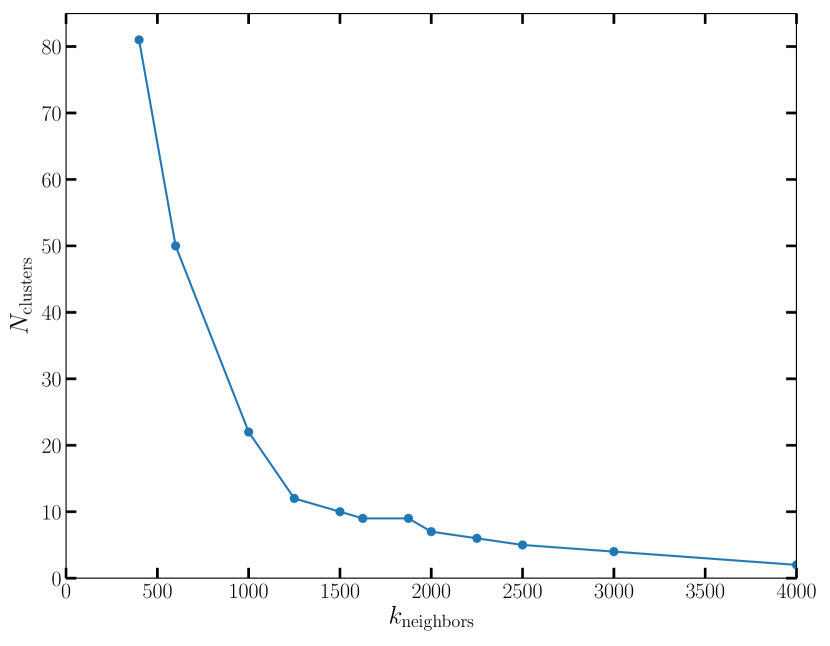
In the Adaptive Meanshift algorithm, controls the size of the adaptive bandwidth of the smoothing kernel: for each datapoint the bandwidth is automatically adjusted to include its nearest neighbours. As a result, this parameter controls the degree of smoothing applied to the PDF gradient estimate, while ensuring equal sampling in the peaks and tails of the PDF.
Most of the time, increasing will result in a decrease in the number of clusters found by the algorithm as local maxima are merged by the increased smoothing. As discussed in Sect. 6.3, too low a value of results in finding artificial maxima caused by the sampling noise. A very large value will smooth the data PDF to a single peak with the shape of the kernel. When decreasing from this large value, the most well separated maxima of the PDF will be distinguished first, then maxima that are weaker or close to the highest maxima.
The first maxima that appear are thus likely to correspond to the strongest physical distinctions, and the following ones to subtler and subtler distinctions (until artificial maxima caused by sampling noise start to appear). As a result, the choice of is mostly a choice of the level of detail we want in our analysis, as long as it is large enough to get rid of sampling noise effects.
Figure 22 shows the variation of the number of clusters found as a function of , for the clustering analysis of the three CO isotopologue lines (cf. Sect. 4). We see a flat plateau close to 10 clusters starting from , indicating that these clusters are more strongly separated than the ones appearing at lower values of (they do not disappear with increased smoothing until much larger smoothing). We thus chose a value corresponding to this plateau.
Appendix C Characteristic intensities in the clusters
| cluster | CO-1 | CO-2 | CO-3 | CO-4 | CO-5 | CO-6 | CO-7 | CO-8 | global | |
|---|---|---|---|---|---|---|---|---|---|---|
| Nb. of pixels | 47440 | 4943 | 14352 | 13336 | 14109 | 24769 | 15625 | 6476 | 141050 | |
| 12CO | center | 1.3 | 13.1 | 20.8 | 37.7 | 45.4 | 56.7 | 59.6 | 93.5 | |
| median | 2.1 | 16.1 | 27.3 | 38.8 | 49.2 | 61.5 | 66.0 | 96.1 | 35.5 | |
| mean | 3.2 | 16.1 | 27.4 | 38.6 | 48.9 | 64.1 | 69.3 | 97.9 | 36.4 | |
| std | 2.9 | 1.9 | 4.8 | 5.0 | 7.2 | 14.6 | 15.6 | 10.5 | 30.3 | |
| 13CO | center | 0.2 | 0.8 | 1.3 | 3.1 | 5.0 | 7.8 | 13.8 | 15.2 | |
| median | 0.3 | 1.0 | 2.1 | 4.2 | 6.1 | 10.4 | 18.1 | 20.8 | 3.6 | |
| mean | 0.4 | 1.1 | 2.2 | 4.4 | 6.3 | 10.4 | 21.5 | 21.5 | 6.6 | |
| std | 0.3 | 0.4 | 0.8 | 1.4 | 1.6 | 2.3 | 9.7 | 5.2 | 8.2 | |
| C18O | center | 0.0 | 0.0 | 0.0 | 0.1 | 0.1 | 0.3 | 0.8 | 0.6 | |
| median | 0.0 | 0.0 | 0.1 | 0.1 | 0.2 | 0.5 | 1.6 | 1.1 | 0.2 | |
| mean | 0.0 | 0.0 | 0.1 | 0.1 | 0.3 | 0.5 | 2.3 | 1.3 | 0.4 | |
| std | 0.1 | 0.1 | 0.1 | 0.2 | 0.2 | 0.3 | 1.7 | 0.6 | 0.9 |
Table C lists characteristic intensity values of the three CO isotopologues for the clusters derived from CO isotopologues only. The values given correspond to the mean, median, standard deviation inside each cluster, as well as the most represented intensity of the cluster (i.e., the PDF local maxima). The cluster’s most represented intensity is generally fainter than the cluster median and mean. This is a natural consequence of the asymmetry of the PDFs that have extended high intensity tails.
Similarly, Table C and C give the characteristic intensity values (median, mean and standard deviation) for the groups of clusters HCO+-1 to 7 and CN-1 to 5.
Appendix D Details of the CO LTE modeling
Here, we describe the details of the modeling that allows us to derive the physical and chemical conditions discussed in Sect. 4.4.
D.1 Parametrization
The intensity integrated over the line profile is defined as
| (10) |
with , 13, and 18 for the , , and (1–0) lines, respectively. In this equation, is the LTE intensity that is defined as
| (11) |
where is the opacity at the line center, is the cosmic microwave background temperature, and ( for (1–0), 5.29 for , and 5.27 for ).
Assuming LTE, we will parametrize the modeled curves with increasing kinetic temperature () at constant opacity
| (12) |
Moreover, we will use the additional freedom to have a higher excitation temperature for , i.e.,
| (13) |
The variation of the opacity with the temperature is computed using the opacity at 20 as reference, i.e.,
| (14) |
| (15) |
| (16) |
where (CO) is the column density of each CO isotopologue (in fact, a lower limit for ), and [CO] is the abundance relative to H2 of each CO isotopologue. Only the can be interpreted in terms of relative abundances because the emission of these isotopologues is probably co-spatial, while the line is mainly sensitive to the foreground part of the emission.
The second factor on the right-hand side of Eq. 10 takes care of the integration over a Gaussian line profile, including the opacity broadening term
| (17) |
where is the measured linewidth of the Gaussian profile for an optically thin line. As we limited the range of velocity over which we integrate the CO lines to , we saturate 0ptij as follows
| (18) |
D.2 Impact of each input parameter
Here, we describe the specific influence that each input parameter has on the curves in the histograms of Fig. 8. At constant opacity, a change of the line FWHM has an homothetic effect on the modeled curves in the intensity vs intensity histograms: the higher the FWHM, the larger the amplitude of the curve. Limiting the interval of velocity over which we integrate quickly leads to a saturation of the integrated intensities. This is the reason why the upper edge of the vs histogram is relatively sharp. This effect is less obvious for the line because the opacity is so large that the line is already saturated. Saturation of the emission also explains the range of observed values of CO isotopologue ratios (bottom left panel). When both and get saturated the intensity ratio is mainly controlled by the ratio of the excitation temperatures, with a modest influence of the opacity broadening term.
The minimum kinetic temperature sets the lower edge of the histogram of vs . Using a lower temperature would result in curves that go beyond the observed minimum intensity for each given intensity. The maximum kinetic temperature controls the regions of low intensities at low column density for all three isotopologues. In other words, we do not populate correctly the low intensity part of the histogram when the maximum temperature is too low.
The column density ratio controls the observed lower edge of the associated intensity vs intensity histogram. A too low value underestimates the intensity at constant intensity and vice versa. In a similar way, the abundance ratio controls the observed upper edge of the associated intensity vs intensity histogram.
Finally, the ratio of the excitation temperatures controls the “width” of the curves. A higher implies both a lower and higher intensity (at low and high value) for the same intensity. In other words, a higher would less well describe both the lower and upper edge of the vs histogram if all other parameters stay constant. A higher also implies a higher slope of the / vs. / curves.
Appendix E Details of the CN, HCO+, and RADEX modeling
Here, we describe the detail of our modeling approach for deriving the HCO+ and CN abundances and abundance ratios discussed in Sect. 5.3.4.
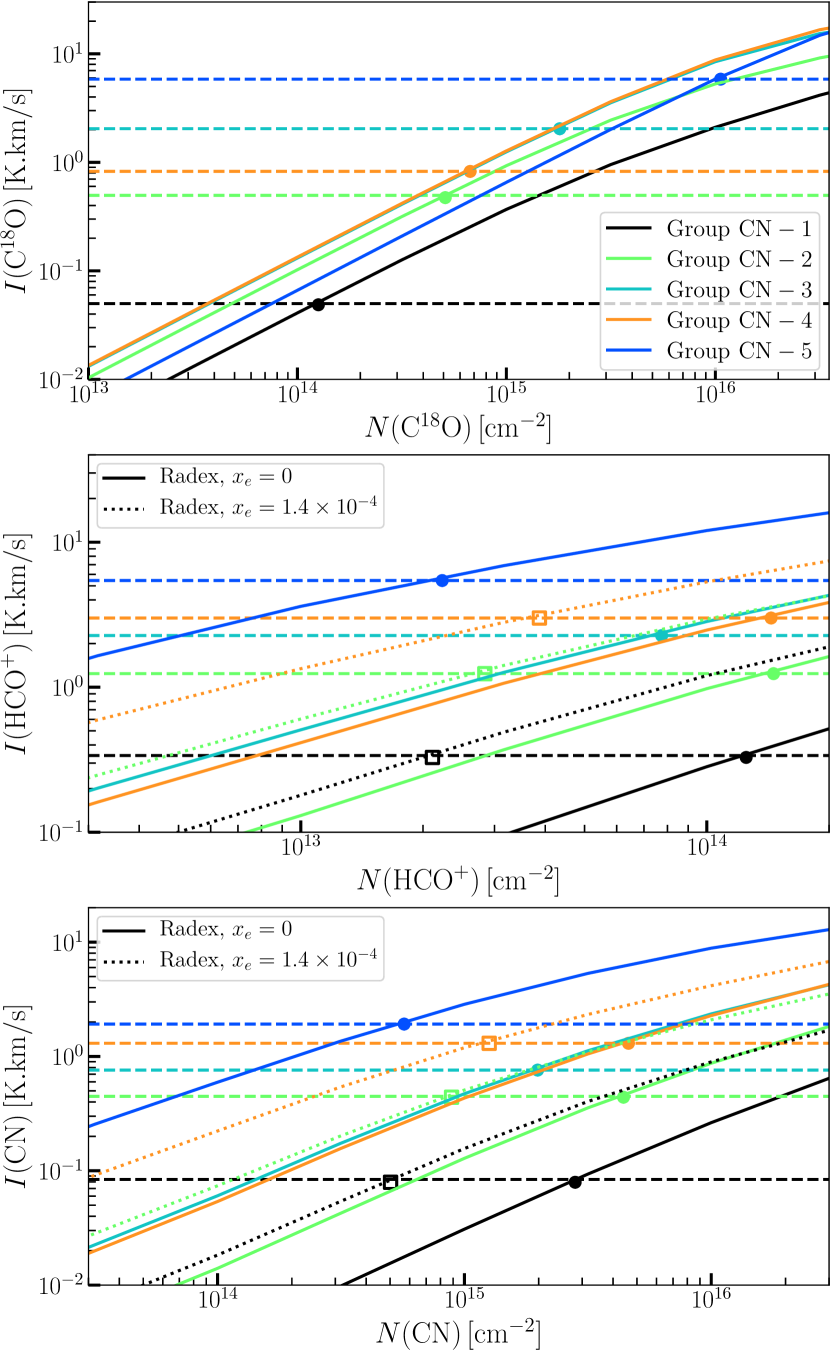
| median | median | median | median C18O | median HCO | median CN | C18O | HCO | CN | |
|---|---|---|---|---|---|---|---|---|---|
| 1 | |||||||||
| 2 | |||||||||
| 3 | |||||||||
| 4 | |||||||||
| 5 |
E.1 RADEX non-LTE radiative transfer models
The radiative transfer modeling is subtle for two reasons. First, the critical densities of C18O, HCO+, and CN (for collisional excitation with H2) differ by two to three orders of magnitude (, , and , respectively). The emission of C18O is mostly thermalized in all groups (except CN-1). In contrast, the excitation of HCO+, and CN is subthermal. We thus use a non-LTE radiative transfer approach. Second, collisions with electrons can dominate the excitation of high dipole moment species such as CN and HCO+ in regions where the electronic fraction is high enough (Black & van Dishoeck 1991; Liszt 2012; Goldsmith & Kauffmann 2017). This effect can be important for the regions of low visual extinction, e.g., groups CN-1 and to a lesser extent CN-2, and for the highly FUV-illuminated PDRs of group CN-4.
We used the RADEX code (van der Tak et al. 2007) which uses the escape probability approach of Sobolev (1960) to compute the non-LTE level populations and the emission from a region of given temperature and volume density of collision partners within a given velocity interval. The position-position-velocity data suggest to use a linewidth of 1. The cross-section coefficients for collisional excitation are obtained from the LAMDA database444http://home.strw.leidenuniv.nl/~moldata/. The coefficient data for collisional excitation of C18O, HCO+, and CN with H2 were computed by Yang et al. (2010), Flower (1999), and Lique et al. (2010), respectively. The data for the excitation by electrons were computed by Faure & Tennyson (2001); Fuente et al. (2008) for HCO+, and Allison & Dalgarno (1971) for CN.
For each CN group, we ran RADEX models for the median values of the volume density and temperature corresponding to each group, and we adjusted the column densities of C18O, HCO+ and CN to best reproduce the median line intensities. As electrons may be important for the collisional excitation of high dipole moment molecules, we used two hypotheses for the electron fraction: (1) The electron fraction is 0 and only H2 contributes to the excitation; (2) The electron fraction is set by the ionisation of all carbon atoms and . Case (2) was computed only for groups where this hypothesis can be relevant : CN-1, 2 and 4. For the diffuse medium of group CN-1, case (2) is a good hypothesis and we take only the corresponding column density values. In group CN-2 and CN-4 however, the electronic fraction is more uncertain, and we give a range of values corresponding to the extreme cases (1) and (2). We assumed a negligible electronic fraction in the other groups.
E.2 Uncertainties
We estimated the uncertainties on the median line intensities by two different methods. First, we used a perturbative Monte Carlo approach. We produced 1000 perturbed datasets (where Gaussian noise is added to each pixel’s intensities according to the local noise rms). We then computed the median intensities inside each group. And we finally took the standard deviation of these results as the uncertainty on the median intensity. Second, we used a bootstrapping method (Feigelson & Babu 2012). We produced 1000 bootstrapped datasets of the same size as the original one (drawing with replacement from the initial dataset). And we took the standard deviation of the medians of these datasets. Both approaches give similar uncertainties. The relative () uncertainties are below 2% for all groups and for the three molecular lines considered here.
Due to the large number of pixels in each group, the median values are highly statistically significant, even in group CN-1 where the three lines stay undetected in most pixels. However, potential unknown biases in the integrated intensities (baseline distortion, etc.) are not taken into account. As a result, the median values for group CN-1 are less reliable than for the other groups. Our estimates of the volume density and kinetic temperature are likely to suffer from global biases. We thus did not try to estimate a noise-associated uncertainty for these quantities.
E.3 Column densities
Figure 23 illustrates how the column densities were derived from the radiative transfer models. Table 4 lists the median input data and the output results. For C18O, the curves of all groups are roughly superimposed (thermalized emission) and the derived column densities are mostly proportional to the median intensities of the groups. In contrast, the intensity vs column density relations are strongly dependent on the median density of the group for HCO+ and CN. For HCO+ and CN, the excitation is subthermal, and closer to the weak excitation regime of Liszt & Pety (2016). As a result, the intensity-column density relations are strongly dependent on the median volume density of the group (in the weak excitation regime, the intensity is proportional to the product of column density and volume density).