Decomposition of Uncertainty in Bayesian Deep Learning
for Efficient and Risk-sensitive Learning

Abstract

Bayesian neural networks with latent variables are scalable and flexible probabilistic models: They account for uncertainty in the estimation of the network weights and, by making use of latent variables, can capture complex noise patterns in the data. We show how to extract and decompose uncertainty into epistemic and aleatoric components for decision-making purposes. This allows us to successfully identify informative points for active learning of functions with heteroscedastic and bimodal noise. Using the decomposition we further define a novel risk-sensitive criterion for reinforcement learning to identify policies that balance expected cost, model-bias and noise aversion.

1 Introduction

Many important problems in machine learning require learning functions in the presence of noise. For example, in reinforcement learning (RL), the transition dynamics of a system is often stochastic. Ideally, a model for these systems should be able to both express such randomness but also to account for the uncertainty in its parameters.

Bayesian neural networks (BNN) are probabilistic models that place the flexibility of neural networks in a Bayesian framework (Blundell et al., 2015; Gal, 2016). In particular, recent work has extended BNNs with latent input variables (BNN+LV) to estimate functions with complex stochasticity such as bimodality or heteroscedasticity (Depeweg et al., 2016). This model class can describe complex stochastic patterns via a distribution over the latent input variables (aleatoric uncertainty), while, at the same time, account for model uncertainty via a distribution over weights (epistemic uncertainty).

In this work we show how to perform and utilize a decomposition of uncertainty in aleatoric and epistemic components for decision making purposes. Our contributions are:

We derive two decompositions that extract epistemic and aleatoric uncertainties from the predictive distribution of BNN+LV (Section 3).

We demonstrate that with this uncertainty decomposition, the BNN+LV identifies informative regions even in bimodal and heteroscedastic cases, enabling efficient active learning in the presence of complex noise (Section 4).

We derive a novel risk-sensitive criterion for model-based RL based on the uncertainty decomposition, enabling a domain expert to trade-off the risks of reliability, which originates from model bias and the risk induced by stochasticity (Section 5). While using uncertainties over transition probabilities to avoid worst-case behavior has been well-studied in discrete MDPs (e.g. (Shapiro & Kleywegt, 2002; Nilim & El Ghaoui, 2005; Bagnell et al., 2001), to our knowledge, our work is the first to consider continuous non-linear functions with complex noise.

2 Background: BNN+LV

We review a recent family of probabilistic models for multi-output regression. These models were previously introduced by Depeweg et al. (2016), we refer to them as Bayesian Neural Networks with latent variables (BNN+LV).

Given a dataset ${\mathcal{D}=\{\mathbf{x}_{n},\mathbf{y}_{n}\}_{n=1}^{N}}$, formed by feature vectors ${\mathbf{x}_{n}\in\mathbb{R}^{D}}$ and targets ${\mathbf{y}_{n}\in\mathbb{R}}^{K}$, we assume that ${\mathbf{y}_{n}=f(\mathbf{x}_{n},z_{n};\mathcal{W})+\bm{\epsilon}_{n}}$, where $f(\cdot,\cdot;\mathcal{W})$ is the output of a neural network with weights $\mathcal{W}$ and $K$ output units. The network receives as input the feature vector $\mathbf{x}_{n}$ and the latent variable $z_{n}\sim\mathcal{N}(0,\gamma)$. We choose rectifiers, ${\varphi(x)=\max(x,0)}$, as activation functions for the hidden layers and the identity function, ${\varphi(x)=x}$, for the output layer. The network output is corrupted by the additive noise variable $\bm{\epsilon}_{n}\sim\mathcal{N}(\bm{0},\bm{\Sigma})$ with diagonal covariance matrix $\bm{\Sigma}$. The role of the latent variable $z_{n}$ is to capture unobserved stochastic features that can affect the network’s output in complex ways. Without $z_{n}$, randomness would only be given by the additive Gaussian observation noise $\bm{\epsilon}_{n}$, which can only describe limited stochastic patterns. The network has $L$ layers, with $V_{l}$ hidden units in layer $l$, and ${\mathcal{W}=\{\mathbf{W}_{l}\}_{l=1}^{L}}$ is the collection of ${V_{l}\times(V_{l-1}+1)}$ weight matrices. The $+1$ is introduced here to account for the additional per-layer biases. We approximate the exact posterior $p(\mathcal{W},\mathbf{z}\,|\,\mathcal{D})$ with:

$$q(\mathcal{W},\mathbf{z})= \underbrace{\left[\prod_{l=1}^{L}\!\prod_{i=1}^{V_{l}}\!\prod_{j=1}^{V_{l\!-\!1}\!+\!1}\mathcal{N}(w_{ij,l}|m^{w}_{ij,l},v^{w}_{ij,l})\right]}_{\text{\small$q(\mathcal{W})$}}\times$$

$$\underbrace{\left[\prod_{n=1}^{N}\mathcal{N}(z_{n}\,|\,m_{n}^{z},v_{n}^{z})\right]}_{\text{\small$q(\mathbf{z})$}}\,.$$ (1)

The parameters $m^{w}_{ij,l}$, $v^{w}_{ij,l}$ and  $m^{z}_{n}$, $v^{z}_{n}$ are determined by minimizing a divergence between $p(\mathcal{W},\mathbf{z}\,|\,\mathcal{D})$ and the approximation $q$. The reader is referred to the work of Hernández-Lobato et al. (2016); Depeweg et al. (2016) for more details on this. In our experiments, we tune $q$ using black-box $\alpha$-divergence minimization with $\alpha=1.0$. While other values of $\alpha$ are possible, this specific value produced better uncertainty decompositions in practice: see Section 4 and the supplementary material for results with $\alpha=0.5$ and $\alpha=0$ (variational Bayes).

BNN+LV can capture complex stochastic patterns, while at the same time account for model uncertainty. They achieve this by jointly learning $q(\mathbf{z})$, which describes the values of the latent variables that were used to generate the training data, and $q(\mathcal{W})$, which represents uncertainty about model parameters. The result is a flexible Bayesian approach for learning conditional distributions with complex stochasticity, e.g. bimodal or heteroscedastic noise.

3 Uncertainty Decomposition in BNN+LV

Let us assume that the targets are one-dimensional, that is, $K=1$. The predictive distribution of a BNN+LV for the target variable $y_{\star}$ associated with the test data point $\mathbf{x}_{\star}$ is

$$p(y_{\star}|\mathbf{x}_{\star})=\int p(y_{\star}|\mathcal{W},\mathbf{x}_{\star},z_{\star})p(z_{\star})q(\mathcal{W})\,dz_{\star}\,d\mathcal{W}\,.$$ (2)

where $p(y_{\star}|\mathcal{W},\mathbf{x}_{\star},z_{\star})=\mathcal{N}(y_{\star}|f(\mathbf{x}_{\star},z_{\star};\mathcal{W}),\bm{\Sigma})$ is the likelihood function, $p(z_{\star})=\mathcal{N}(z_{\star}|0,\gamma)$ is the prior on the latent variables and $q(\mathcal{W})$ is the approximate posterior for $\mathcal{W}$ given $\mathcal{D}$. In this expression $q(\mathbf{z})$ is not used since the integration with respect to $z_{\star}$ must be done using the prior $p(z_{\star})$. The reason for this is that the $y_{\star}$ associated with $\mathbf{x}_{\star}$ is unknown and consequently, there is no other evidence on $z_{\star}$ than the one coming from $p(z_{\star})$.

In Eq. (2), the randomness or uncertainty on $y_{\star}$ has its origin in $\mathcal{W}\sim q(\mathcal{W})$, $z_{\star}\sim p(z_{\star})$ and $\epsilon\sim\mathcal{N}(0,\sigma^{2})$. This means that there are two types of uncertainties entangled in our predictons for $y_{\star}$: aleatoric and epistemic (Der Kiureghian & Ditlevsen, 2009; Kendall & Gal, 2017). The aleatoric uncertainty originates from the randomness of $z_{\star}$ and $\epsilon$ and cannot be reduced by collecting more data. By contrast, the epistemic uncertainty originates from the randomness of $\mathcal{W}$ and can be reduced by collecting more data, which will typically shrink the approximate posterior $q(\mathcal{W})$.

Eq. (2) is the tool to use when making predictions for $y_{\star}$. However, there are many settings in which, for decision making purposes, we may be interested in separating the two forms of uncertainty present in this distribution. We now describe two decompositions , each one differing in the metric used to quantify uncertainty: the first one is based on the entropy, whereas the second one uses the variance.

Let $\text{H}(\cdot)$ compute the differential entropy of a probability distribution. The total uncertainty present in Eq. (2) can then be quantified as $\text{H}(y_{\star}|\mathbf{x}_{\star})$. Furthermore, assume that we do not integrate $\mathcal{W}$ out in Eq. (2) and, instead, we just condition on a specific value of this variable. The result is then $p(y_{\star}|\mathcal{W},\mathbf{x}_{\star})=\int p(y_{\star}|\mathcal{W},\mathbf{x}_{\star},z_{\star})p(z_{\star})\,dz_{\star}$ with corresponding uncertainty $\text{H}(y_{\star}|\mathcal{W},\mathbf{x}_{\star})$. The expectation of this quantity under $q(\mathcal{W})$, that is, $\mathbf{E}_{q(\mathcal{W})}[\text{H}(y_{\star}|\mathcal{W},\mathbf{x}_{\star})]$, can then be used to quantify the overall uncertainty in Eq. (2) coming from $z_{\star}$ and $\epsilon$. Therefore, $\mathbf{E}_{q(\mathcal{W})}[\text{H}(y_{\star}|\mathcal{W},\mathbf{x}_{\star})]$, measures the aleatoric uncertainty. We can then quantify the epistemic part of the uncertainty in Eq. (2) by computing the difference between total and aleatoric uncertainties:

$$\text{H}[y_{\star}|\mathbf{x}_{\star}]-\mathbf{E}_{q(\mathcal{W})}[\text{H}(y_{\star}|\mathcal{W},\mathbf{x}_{\star})]=I(y_{\star},\mathcal{W})\,,$$ (3)

which is the mutual information between $y_{\star}$ and $\mathcal{W}$.

Instead of the entropy, we can use the variance as a measure of uncertainty. Let $\sigma^{2}(\cdot)$ compute the variance of a probability distribution. The total uncertainty present in Eq. (2) is then $\sigma^{2}(y_{\star}|\mathbf{x}_{\star})$. This quantity can then be decomposed using the law of total variance:

$$\sigma^{2}(y_{\star}|\mathbf{x}_{\star}) =\sigma^{2}_{q(\mathcal{W})}(\mathbf{E}[y_{\star}|\mathcal{W},\mathbf{x}_{\star}])+\mathbf{E}_{q(\mathcal{W})}[\sigma^{2}(y_{\star}|\mathcal{W},\mathbf{x}_{\star})]\,.$$

where $\mathbf{E}[y_{\star}|\mathcal{W},\mathbf{x}_{\star}]$ and $\sigma^{2}[y_{\star}|\mathcal{W},\mathbf{x}_{\star}]$ are, respectively, the mean and variance of $y_{\star}$ according to $p(y_{\star}|\mathcal{W},\mathbf{x}_{\star})$. In the expression above, $\sigma^{2}_{q(\mathcal{W})}(\mathbf{E}[y_{\star}|\mathcal{W},\mathbf{x}_{\star}])$ is the variance of $\mathbf{E}[y_{\star}|\mathcal{W},\mathbf{x}_{\star}]$ when $\mathcal{W}\sim q(\mathcal{W})$. This term ignores any contribution to the variance of $y_{\star}$ from $z_{\star}$ and $\epsilon$ and only considers the effect of $\mathcal{W}$. Therefore, it corresponds to the epistemic uncertainty in Eq. (2). By contrast, the term $\mathbf{E}_{q(\mathcal{W})}[\sigma^{2}(y_{\star}|\mathcal{W},\mathbf{x}_{\star})]$ represents the average value of $\sigma^{2}(y_{\star}|\mathcal{W},\mathbf{x}_{\star})$ when $\mathcal{W}\sim q(\mathcal{W})$. This term ignores any contribution to the variance of $y_{\star}$ from $\mathcal{W}$ and, therefore, it represents the aleatoric uncertainty in Eq. (2).

In some cases, working with variances can be undesirable because they have square units. To avoid this problem, we can work with the square root of the previous terms. For example, we can represent the total uncertainty using

$$\sigma(y_{\star}|\mathbf{x}_{\star})=$$

$$\quad\quad\left\{\sigma^{2}_{q(\mathcal{W})}(\mathbf{E}[y_{\star}|\mathcal{W},\mathbf{x}_{\star}])+\mathbf{E}_{q(\mathcal{W})}[\sigma^{2}(y_{\star}|\mathcal{W},\mathbf{x}_{\star})]\right\}^{\frac{1}{2}}\,.$$ (4)

4 Active Learning with Complex Noise

Active learning is the problem of iteratively collecting data so that the final gains in predictive performance are as high as possible (Settles, 2012). We consider the case of actively learning arbitrary non-linear functions with complex noise. To do so, we apply the information-theoretic framework for active learning described by MacKay (1992), which is based on the reduction of entropy in the model’s posterior distribution. Below, we show that this framework naturally results in the entropy-based uncertainty decomposition from Section 3. Next, we demonstrate how this framework, applied to BNN+LV enables data-efficient learning in the presence of heteroscedastic and bimodal noise.

Assume a BNN+LV is used to describe a batch of training data $\mathcal{D}=\{(\mathbf{x}_{1},\mathbf{y}_{1}),\cdots,(\mathbf{x}_{N},\mathbf{y}_{N})\}$. The expected reduction in posterior entropy for $\mathcal{W}$ that would be obtained when collecting the unknown target $\mathbf{y}_{\star}$ for the input $\mathbf{x}_{\star}$ is

$$\text{H}(\mathcal{W}|\mathcal{D})- \mathbf{E}_{\mathbf{y}_{\star}|\mathbf{x}_{\star},\mathcal{D}}\left[\text{H}(\mathcal{W}|\mathcal{D}\cup\{\mathbf{x}_{\star},\mathbf{y}_{\star}\})\right]=I(\mathcal{W},\mathbf{y}_{\star})$$

$$=\text{H}(\mathbf{y}_{\star}|\mathbf{x}_{\star})-\mathbf{E}_{q(\mathcal{W})}\left[\text{H}(\mathbf{y}_{\star}|\mathcal{W},\mathbf{x}_{\star})\right]\,.$$ (5)

Note that this is the epistemic uncertainty that we introduced in Section 3, which has arisen naturally in this setting: the most informative $\mathbf{x}_{\star}$ for which to collect $y_{\star}$ next is the one for which the epistemic uncertainty in the BNN+LV predictive distribution is the highest.

The epistemic uncertainty in Eq. (5) can be approximated using standard entropy estimators, e.g. nearest-neighbor methods (Kozachenko & Leonenko, 1987; Kraskov et al., 2004; Gao et al., 2016). For that, we repeatedly sample $\mathcal{W}$ and $z_{\star}$ and do forward passes through the BNN+LV to sample $\mathbf{y}_{\star}$. The resulting samples of $\mathbf{y}_{\star}$ can then be used to approximate the respective entropies for each $\mathbf{x}_{\star}$ using the nearest-neighbor approach:

$$\text{H}(\mathbf{y}_{\star}|\mathbf{x}_{\star})-\mathbf{E}_{q(\mathcal{W})}\left[\text{H}(\mathbf{y}_{\star}|\mathcal{W},\mathbf{x}_{\star})\right]$$

$$\approx\hat{\text{H}}(\mathbf{y}_{\star}^{1},\ldots,\mathbf{y}^{L}_{\star})-\frac{1}{M}\sum_{i=1}^{M}\left[\hat{\text{H}}(\mathbf{y}_{\star}^{1,\mathcal{W}_{i}},\ldots,\mathbf{y}_{\star}^{L,\mathcal{W}_{i}})\right]\,.$$ (6)

where $\hat{\text{H}}(\cdot)$ is a nearest-neighbor entropy estimate given an empirical sample of points, $\mathbf{y}_{\star}^{1},\ldots,\mathbf{y}_{\star}^{L}$ are sampled from $p(\mathbf{y}_{\star}|\mathbf{x}_{\star})$ according to Eq. (2), $\mathcal{W}_{1},\ldots,\mathcal{W}_{M}\sim q(\mathcal{W})$ and $\mathbf{y}_{\star}^{1,\mathcal{W}_{i}},\ldots,\mathbf{y}_{\star}^{L,\mathcal{W}_{i}}\sim p(y_{\star}|\mathcal{W}_{i},\mathbf{x}_{\star})$ for $i=1,\ldots,M$.

There are alternative ways to estimate the entropy, e.g. with histograms or using kernel density estimation (KDE) (Beirlant et al., 1997). We choose nearest neighbor methods because they tend to work well in low dimensions, are fast to compute (compared to KDE) and do not require much hyperparameter tuning (compared to histograms). However, we note that for high-dimensional problems, estimating entropy is a difficult problem.

4.1 Experiments

We evaluate the active learning procedure on three problems. In each of them, we first train a BNN+LV with 2 hidden layers and 20 units per layer. Afterwards, we approximate the epistemic uncertainty as outlined in the previous section. Hyper-parameter settings and details for replication can be found in the supplementary material, which includes results for three other inference methods: Hamiltonian Monte Carlo (HMC), black-box $\alpha$- divergence minimization with $\alpha=0.5$ and $\alpha=0$ (variational Bayes). These results show that the decomposition of uncertainty produced by $\alpha=1$ and the gold standard HMC are similar, but for lower values of $\alpha$ this is not the case. Our main findings are:

The decomposition of uncertainty allows us to identify informative inputs when the noise is heteroscedastic.

We consider a regression problem with heteroscedastic noise where $y=7\sin(x)+3|\cos(x/2)|\epsilon$ with $\epsilon\sim\mathcal{N}(0,1)$. We sample 750 values of the input $x$ from a mixture of three Gaussians with mean parameters $\{\mu_{1}=-4,\mu_{2}=0,\mu_{3}=4\}$, variance parameters $\{\sigma_{1}=\frac{2}{5},\sigma_{2}=0.9,\sigma_{3}=\frac{2}{5}\}$ and with each Gaussian component having weight equal to $1/3$ in the mixture. Figure 1a shows the data. We have many points at the borders and in the center, but few in between.

(a)

(b)

(c)

(d)

(e)

(f)

Figure 1: Uncertainty decomposition on heteroscedastic data. LABEL:sub@fig:rd: Raw data. LABEL:sub@fig:dd: Density of $x$ in data. LABEL:sub@fig:pd: Predictive distribution $p(y_{\star}|x_{\star})$. LABEL:sub@fig:h: Estimate of $\text{H}(y_{\star}|x_{\star})$. LABEL:sub@fig:hgw: Estimate of $\mathbf{E}_{q(\mathcal{W})}\left[\text{H}(y_{\star}|x_{\star},\mathcal{W})\right]$. LABEL:sub@fig:ob: Estimate of entropy reduction $\text{H}(y_{\star}|x_{\star})-\mathbf{E}_{q(\mathcal{W})}\left[\text{H}(y_{\star}|x_{\star},\mathcal{W})\right]$.

(a)

(b)

(c)

(d)

(e)

(f)

Figure 2: Uncertainty decomposition on bimodal data. LABEL:sub@fig:rd: Raw data. LABEL:sub@fig:dd: Density of $x$ in data. LABEL:sub@fig:pd: Predictive distribution: $p(y_{\star}|x_{\star})$. LABEL:sub@fig:h: Estimate of $\text{H}(y_{\star}|x_{\star})$. LABEL:sub@fig:hgw: Estimate of $\mathbf{E}_{q(\mathcal{W})}\left[\text{H}(y_{\star}|x_{\star},\mathcal{W})\right]$. LABEL:sub@fig:ob: Estimate of entropy reduction $\text{H}(y_{\star}|x_{\star})-\mathbf{E}_{q(\mathcal{W})}\left[\text{H}(y_{\star}|x_{\star},\mathcal{W})\right]$.

(a)

(b)

(c)

(d)

Figure 3: Uncertainty decomposition on wet-chicken dynamics. LABEL:sub@fig:wcrd: Raw data. LABEL:sub@fig:wch: Entropy estimate $\text{H}(\mathbf{s}_{t+1}|\mathbf{s}_{t})$ of predictive distribution for each $\mathbf{s}_{t}$ (using $\mathbf{a}_{t}=\{0,0\}$). LABEL:sub@fig:hgw: Conditional entropy estimate $\mathbf{E}_{q(\mathcal{W})}\left[\text{H}(\mathbf{s}_{t+1}|\mathbf{s}_{t},\mathcal{W})\right]$. LABEL:sub@fig:ob: Estimated entropy reduction.

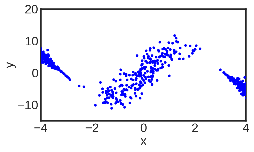
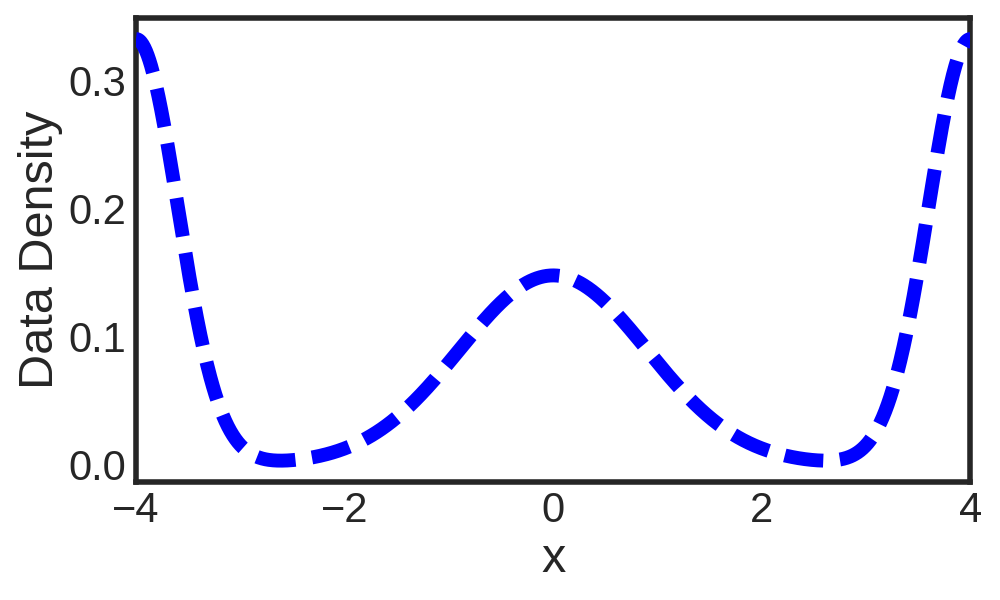
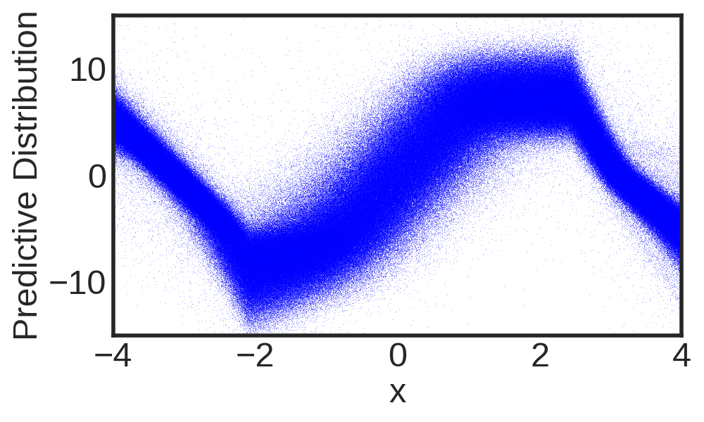
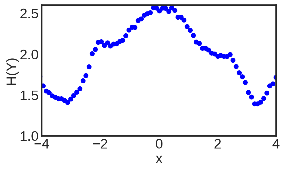
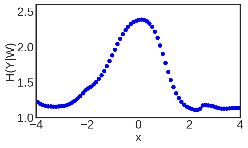
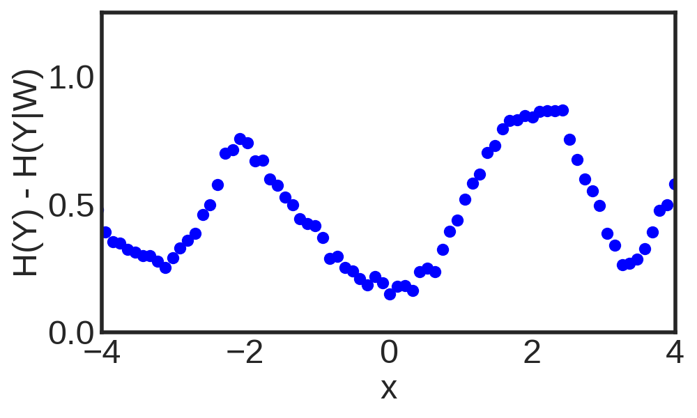
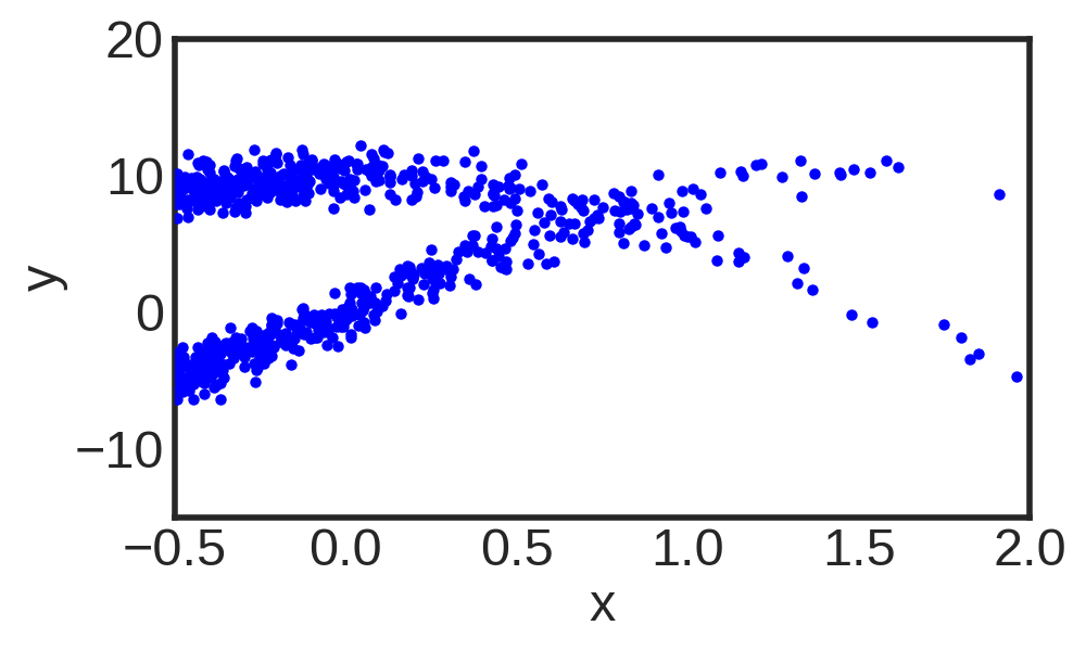
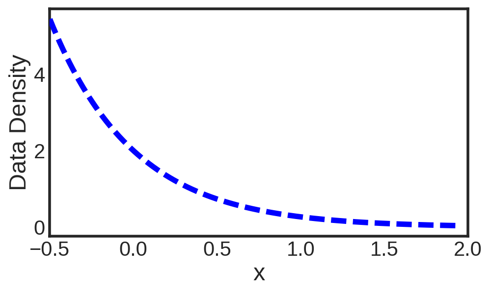
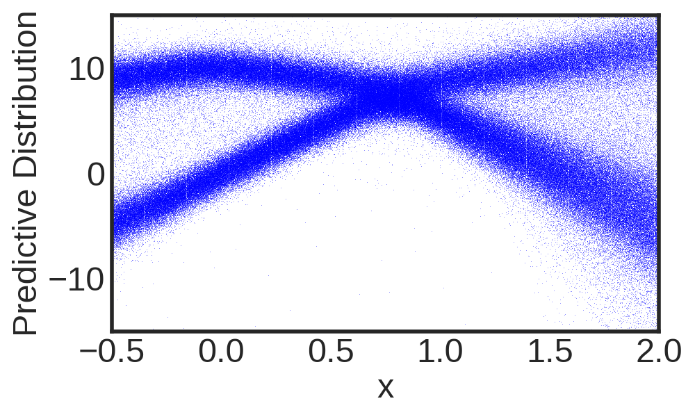
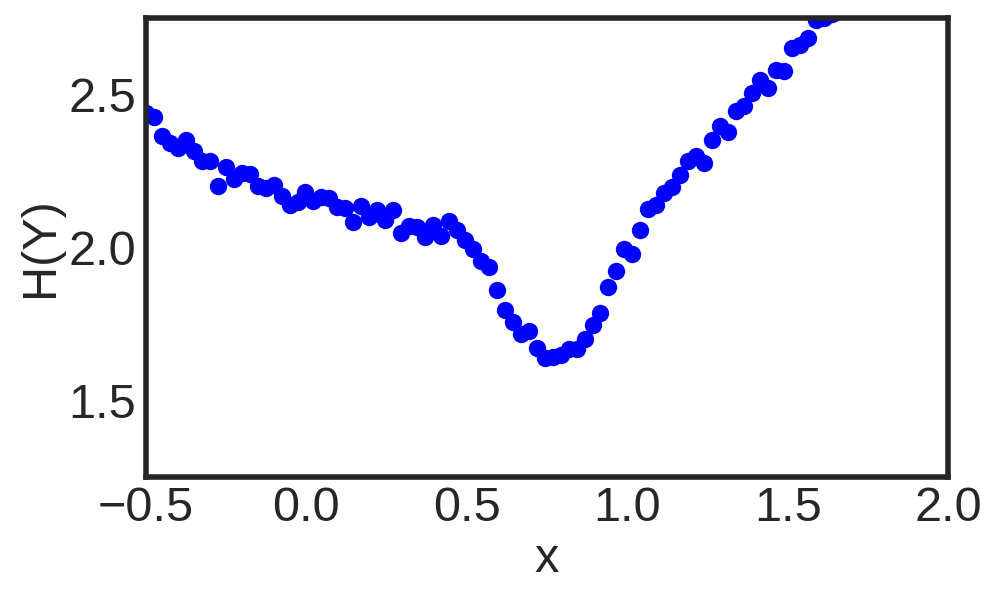
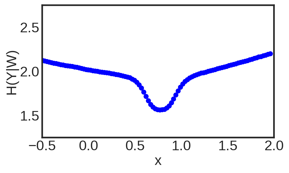
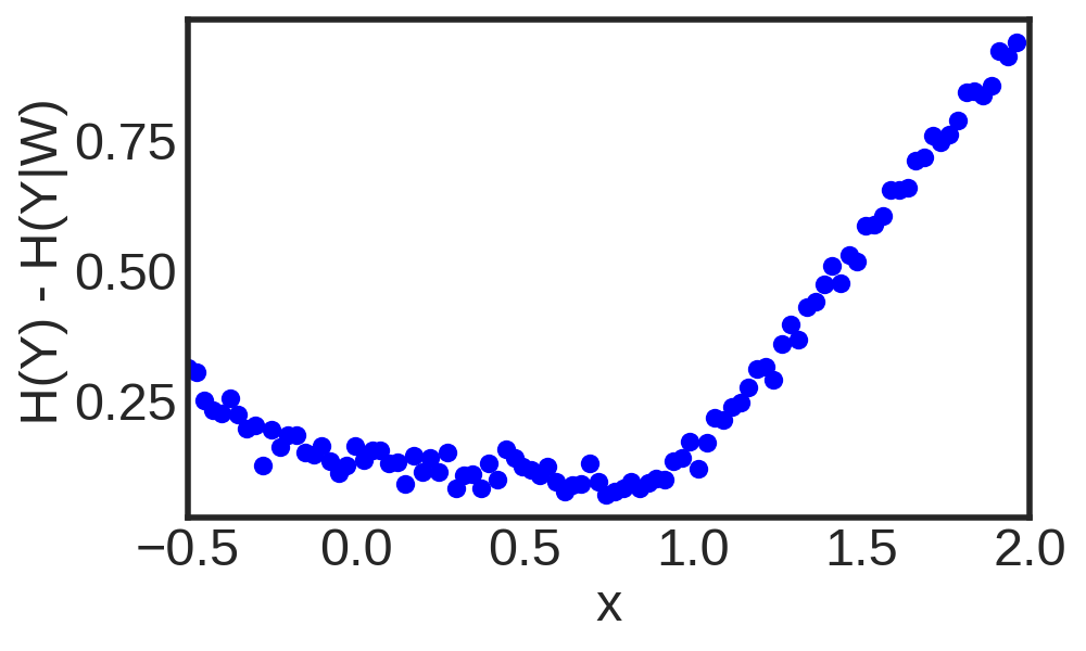
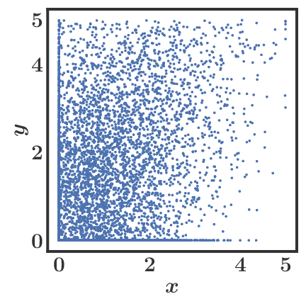
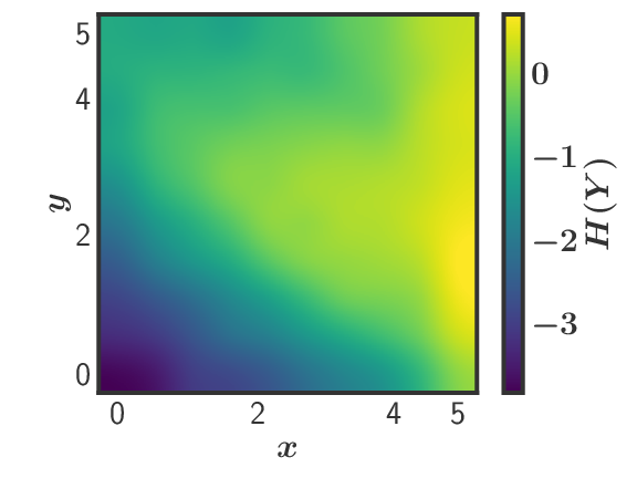
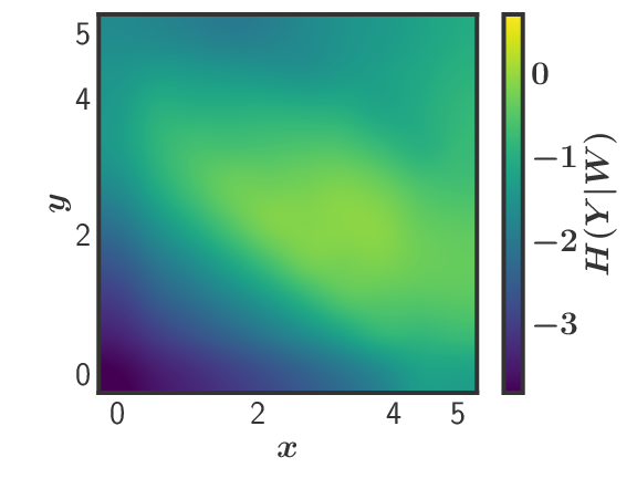
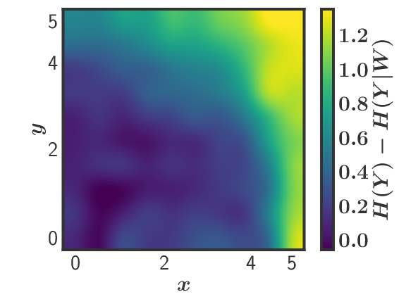
Figure 1 shows the results obtained (see caption for details). The resulting decomposition of predictive uncertainty is very accurate: the epistemic uncertainty (Figure 1f), is inversely proportional to the density used to sample the data (Figure 1b). This makes sense, since in this toy problem the most informative inputs are located in regions where data is scarce. However, this may not be the case in more complicated settings. Finally, we note that the total predictive uncertainty (Figure 1d) fails to identify informative regions.

The decomposition of uncertainty allows us to identify informative inputs when the noise is bimodal.

Next we consider a toy problem given by a regression task with bimodal data. We define $x\in[-0.5,2]$ and $y=10\sin(x)+\epsilon$ with probability $0.5$ and $y=10\cos(x)+\epsilon$, otherwise, where $\epsilon\sim\mathcal{N}(0,1)$ and $\epsilon$ is independent of $x$. We sample 750 values of $x$ from an exponential distribution with $\lambda=2$. Figure 2a shows the data. We have many points on the left, but few on the right.

Figure 2 shows the results obtained (see caption for details). Figure 2c shows that the BNN+LV has learned the bimodal structure in the data and Figure 2d shows how the total predictive uncertainty increases on the right, where data is scarce. The aleatoric uncertainty (Figure 2e), by contrast, has an almost symmetric form around $x=0.75$, taking lower values at this location. This makes sense since the data generating process is symmetric around $x=0.75$ and the noise changes from bimodal to unimodal when one gets closer to $x=0.75$. Figure 2f shows an estimate of the epistemic uncertainty, which as expected increases with $x$.

The decomposition of uncertainty identifies informative inputs when noise is both heteroscedastic and bimodal.

We consider data sampled from a 2D stochastic system called the wet-chicken (Hans & Udluft, 2009; Depeweg et al., 2016), see the supplementary material for details. The wet-chicken transition dynamics exhibit complex stochastic patterns: bimodality, heteroscedasticity and truncation (the agent cannot move beyond the boundaries of state space: $[0,5]^{2}$). The data are $7,500$ state transitions collected by random exploration. Figure 3a shows the states visited. For each transition, the BNN+LV predicts the next state given the current one and the action applied. Figure 3d shows that the epistemic uncertainty is highest in the top right corner, while data is most scarce in the bottom right corner. The reason for this result is that the wet-chicken dynamics bring the agent back to $y=0$ whenever the agent goes beyond $y=5$, but this does not happen for $y=0$ where the agent just bounces back. Therefore, learning the dynamics is more difficult and requires more data at $y=5$ than at $y=0$. The epistemic uncertainty captures this property, but the total predictive uncertainty (Figure 3b) does not.

	Method
Dataset	$I_{\text{bb-$\alpha$}}(\mathcal{W},y_{\star})$		$\text{H}_{\text{bb-}\alpha}(\mathbf{y}_{\star}|\mathbf{x}_{\star})$		GP
Heteroscedastic	-1.79$\pm$	0.03	-1.92$\pm$	0.03	-2.09$\pm$	0.02
Bimodal	-2.04$\pm$	0.01	-2.06$\pm$	0.02	-2.86$\pm$	0.01
Wet-chicken	1.18$\pm$	0.16	0.57$\pm$	0.20	-3.22$\pm$	0.03

Table 1: Test log-likelihood in active learning experiments after $150$ iterations.

Active learning with BBN+LV is improved by using the uncertainty decomposition.

We evaluate the gains obtained by using Eq. (5) with BNN+LV, when collecting data in three toy active learning problems. We refer to this method as $I_{\text{bb-$\alpha$}}(\mathcal{W},y_{\star})$ and compare it with two baselines. The first one also uses a BNN+LV to describe data, but does not perform a decomposition of predictive uncertainty, that is, this method uses $\text{H}(\mathbf{y}_{\star}|\mathbf{x}_{\star})$ instead of Eq. (5) for active learning. We call this method $\text{H}_{\text{bb-}\alpha}(\mathbf{y}_{\star}|\mathbf{x}_{\star})$. The second baseline is given by a Gaussian process (GP) model which collects data according to $\text{H}(\mathbf{y}_{\star}|\mathbf{x}_{\star})$ since in this case the uncertainty decomposition is not necessary because the GP model does not include latent variables. The GP model assumes Gaussian noise and is not able to capture complex stochastic patterns.

The three problems considered correspond to the datasets from Figures 1, 2 and 3. The general set-up is as follows. We start with the available data shown in the previous figures. At each iteration, we select a batch of data points to label from a pool set which is sampled uniformly at random in input space. The selected data is then included in the training set and the log-likelihood is evaluated on a separate test set. This process is performed for $150$ iterations and we repeat all experiments 5 times.

Table 1 shows the results obtained. Overall, BNN+LV outperform GPs in terms of predictive performance. We also see significant gains of $I_{\text{bb-$\alpha$}}(\mathcal{W},y_{\star})$ over $\text{H}(\mathbf{y}_{\star}|\mathbf{x}_{\star})$ on the heteroscedastic and wet-chicken tasks, whereas their results are similar on the bimodal task. The reason for this is that, in the latter task, the epistemic and the total uncertainty have a similar behaviour as shown in Figures 2d and 2f. Finally, we note that heteroscedastic GPs (Le et al., 2005) will likely perform similar to BNN+LV in the heteroscedastic task from Figure 2, but they will fail in the other two settings considered (Figures 2 and 3).

5 Risk-sensitive Reinforcement Learning

We propose an extension of the “risk-sensitive criterion” for safe model-based RL (García & Fernández, 2015) to balance the risks produced by epistemic and aleatoric uncertainties.

We focus on batch RL with continuous state and action spaces (Lange et al., 2012): we are given a batch of state transitions $\mathcal{D}=\{(\mathbf{s}_{t},\mathbf{a}_{t},\mathbf{s}_{t+1})\}$ formed by triples containing the current state $\mathbf{s}_{t}$, the action applied $\mathbf{a}_{t}$ and the next state $\mathbf{s}_{t+1}$. In addition to $\mathcal{D}$, we are also given a cost function $c$. The goal is to obtain from $\mathcal{D}$ a policy in parametric form that minimizes $c$ on average under the system dynamics.

In model-based RL, the first step consists in learning a dynamics model from $\mathcal{D}$. We assume that the true dynamical system can be expressed by an unknown neural network with latent variables:

$$\mathbf{s}_{t}=f_{\text{true}}(\mathbf{s}_{t-1},\mathbf{a}_{t-1},z_{t};\mathcal{W}_{\text{true}})\,,\quad z_{t}\sim\mathcal{N}(0,\gamma)\,,$$ (7)

where $\mathcal{W}_{\text{true}}$ denotes the weights of the network and $\mathbf{s}_{t-1}$, $\mathbf{a}_{t-1}$ and $z_{t}$ are the inputs to the network. We use BNN+LV from Section 2 to approximate a posterior $q(\mathcal{W},z)$ using the batch $\mathcal{D}$ (Depeweg et al., 2016).

In model-based policy search we optimize a policy given by a deterministic neural network with weights $\mathcal{W}_{\pi}$. This parametric policy returns an action $\mathbf{a}_{t}$ as a function of $\mathbf{s}_{t}$, that is, $\mathbf{a}_{t}=\pi(\mathbf{s}_{t};\mathcal{W}_{\pi})$. The policy parameters $\mathcal{W}_{\pi}$ can be tuned by minimizing the expectation of the cost $C=\sum_{t=1}^{T}c_{t}$ over a finite horizon $T$ with respect to the belief $q(\mathcal{W})$, where $c_{t}=c(\mathbf{s}_{t})$. This expected cost is obtained by averaging across multiple virtual roll-outs as described next.

Given $\mathbf{s}_{0}$, we sample $\mathcal{W}\sim q$ and simulate state trajectories for $T$ steps using the model $\mathbf{s}_{t+1}=f(\mathbf{s}_{t},\mathbf{a}_{t},z_{t};\mathcal{W})+\bm{\epsilon}_{t+1}$ with policy $\mathbf{a}_{t}=\pi(\mathbf{s}_{t};\mathcal{W}_{\pi})$, input noise $z_{t}\sim\mathcal{N}(0,\gamma)$ and additive noise $\bm{\epsilon}_{t+1}\sim\mathcal{N}(\bm{0},\bm{\Sigma})$. By averaging across these roll-outs, we obtain a Monte Carlo approximation of the expected cost given the initial state $\mathbf{s}_{0}$:

$$\textstyle J(\mathcal{W}_{\pi})=\textstyle\mathbf{E}\left[C\right]=\textstyle\mathbf{E}\left[\sum_{t=1}^{T}c_{t}\right]\,,$$ (8)

where, $\mathbf{E}[\cdot]$ denotes here an average across virtual roll-outs starting from $\mathbf{s}_{0}$ and, to simplify our notation, we have made the dependence on $\mathbf{s}_{0}$ implicit. The policy search algorithm optimizes the expectation of Eq. (8) when $\mathbf{s}_{0}$ is sampled uniformly from $\mathcal{D}$, that is, $\mathbf{E}_{\mathbf{s}_{0}\sim\mathcal{D}}[J(\mathcal{W}_{\pi})]$. This quantity can be easily approximated by Monte Carlo and if model, policy, and cost function are differentiable, we are able to tune $\mathcal{W}_{\pi}$ by stochastic gradient descent.

The “risk-sensitive criterion” (García & Fernández, 2015) changes Eq. (8) to atain a balance between expected cost and risk, where the risk typically penalizes the deviations of $C$ from $\mathbf{E}[C]$ during the virtual roll-outs with initial state $\mathbf{s}_{0}$. For example, the risk-sensitive objective could be

$$\textstyle J(\mathcal{W}_{\pi})=\textstyle\mathbf{E}\left[C\right]+\beta\mathbf{\sigma}(C)\,,$$ (9)

where $\mathbf{\sigma}(C)$ is the standard deviation of $C$ across virtual roll-outs starting from $\mathbf{s}_{0}$ and the risk-sensitive parameter $\beta$ determines the amount of risk-avoidance ($\beta\geq 0$) or risk-seeking behavior ($\beta<0$) when optimizing $\mathcal{W}_{\pi}$.

Instead of working directly with the risk on the final cost $C$, we consider the sum of risks on the individual costs $c_{1},\ldots,c_{T}$. The reason for this is that the latter is a more restrictive criterion since low risk on the $c_{t}$ will imply low risk on $C$, but not the other way around. Let $\sigma(c_{t})$ denote the standard deviation of $c_{t}$ over virtual roll-outs starting from $\mathbf{s}_{0}$. We can then explicitly write $\sigma(c_{t})$ in terms of its aleatoric and epistemic components by using the decomposition of uncertainty from Eq. (4). In particular,

$$\sigma(c_{t})=\left\{\sigma^{2}_{q(\mathcal{W})}(\mathbf{E}[c_{t}|\mathcal{W}])+\mathbf{E}_{q(\mathcal{W})}[\sigma^{2}(c_{t}|\mathcal{W})]\right\}^{\frac{1}{2}}\,,$$ (10)

where $\mathbf{E}[c_{t}|\mathcal{W}]$ and $\sigma^{2}(c_{t}|\mathcal{W})$ denote the mean and variance of $c_{t}$ under virtual roll-outs from $\mathbf{s}_{0}$ performed with policy $\mathcal{W}_{\pi}$ and under the dynamics of a BNN+LV with parameters $\mathcal{W}$. In a similar manner as in Eq. (4), the operators $\mathbf{E}_{q(\mathcal{W})}[\cdot]$ and $\sigma^{2}_{q(\mathcal{W})}(\cdot)$ in Eq. (10) compute the mean and variance of their arguments when $\mathcal{W}\sim q(\mathcal{W})$.

The two terms inside the square root in Eq. (10) have a clear interpretation. The first one, $\mathbf{E}_{q(\mathcal{W})}[\sigma^{2}(c_{t}|\mathcal{W})]$, represents the risk originating from the sampling of $z$ and $\bm{\epsilon}$ in the virtual roll-outs. We call this term the aleatoric risk. The second term, $\sigma^{2}_{q(\mathcal{W})}(\mathbf{E}[c_{t}|\mathcal{W}])$, encodes the risk originating from the sampling of $\mathcal{W}$ in the virtual roll-outs. We call this term the epistemic risk.

We can now extend the objective in Eq. (8) with a new risk term that balances the epistemic and aleatoric risks. This term is obtained by first using risk-sensitive parameters $\beta$ and $\gamma$ to balance the epistemic and aleatoric components in Eq. (10), and then summing the resulting expression for $t=1,\ldots,T$:

$$\sigma(\gamma,\beta)=\sum_{t=1}^{T}\left\{\beta^{2}\sigma^{2}_{q(\mathcal{W})}(\mathbf{E}[c_{t}|\mathcal{W}])+\gamma^{2}\mathbf{E}_{q(\mathcal{W})}[\sigma^{2}(c_{t}|\mathcal{W})]\right\}^{\frac{1}{2}}\,.$$

Therefore, our ‘risk-sensitive criterion” uses the function $J(\mathcal{W}_{\pi})=\mathbf{E}\left[C\right]+\sigma(\gamma,\beta)$, which can be approximated via Monte Carlo and optimized using stochastic gradient descent. The Monte Carlo approximation is generated by performing $M\times N$ roll-outs with starting state $\mathbf{s}_{0}$ sampled uniformly from $\mathcal{D}$. For this, $\mathcal{W}$ is sampled from $q(\mathcal{W})$ a total of $M$ times and then, for each of these samples, $N$ roll-outs are performed with $\mathcal{W}$ fixed and sampling only the latent variables and the additive Gaussian noise in the BBN+LV. Let $z_{t}^{m,n}$ and $\bm{\epsilon}_{t}^{m,n}$ be the samples of the latent variables and the additive Gaussian noise at step $t$ during the $n$-th roll-out for the $m$-th sample of $\mathcal{W}$, which we denote by $\mathcal{W}^{m}$. Then $c_{m,n}(t)=c(\mathbf{s}_{t}^{\mathcal{W}^{m},\{z_{1}^{m,n},\ldots,z_{t}^{m,n}\},\{\bm{\epsilon}_{1}^{m,n},\ldots,\bm{\epsilon}_{t}^{m,n}\},\mathcal{W}_{\pi}})$ denotes the cost obtained at time $t$ in that roll-out. All these cost values obtained at time $t$ are stored in the $M\times N$ matrix $\mathbf{C}(t)$. The Monte Carlo estimate of $J(\mathcal{W}_{\pi})$ is then

$$J(\mathcal{W}_{\pi})\approx\sum_{t=1}^{T}\bigg{\{}\frac{\mathbf{1}^{\text{T}}\mathbf{C}(t)\mathbf{1}}{MN}+$$

$$\left\{\beta^{2}\hat{\sigma}^{2}\left[\mathbf{C}(t)\mathbf{1}/N\right]+\gamma^{2}\frac{1}{M}\sum_{m=1}^{M}\hat{\sigma}^{2}\left[\mathbf{C}(t)_{m,\cdot}\right]\right\}^{\frac{1}{2}}\bigg{\}}\,,$$ (11)

where $\mathbf{1}$ denotes a vector with all of its entries equal to 1, $\mathbf{C}(t)_{m,\cdot}$ is a vector with the $m$-th row of $\mathbf{C}(t)$ and $\hat{\sigma}^{2}[\mathbf{x}]$ returns the empirical variance of the entries in vector $\mathbf{x}$.

By setting $\beta$ and $\gamma$ to specific values in Eq. (11), the user can choose different trade-offs between cost, aleatoric and epistemic risk: for $\gamma=0$ the term inside the square root is $\beta^{2}$ times $\hat{\sigma}^{2}\left[\mathbf{C}(t)\mathbf{1}/N\right]$ which is a Monte Carlo approximation of the epistemic risk in Eq. (10). Similarly, for $\beta=0$, inside the square root we obtain $\gamma^{2}$ times $\frac{1}{M}\sum_{m=1}^{M}\hat{\sigma}^{2}\left[\mathbf{C}(t)_{m,\cdot}\right]$ which approximates the aleatoric risk. For $\beta=\gamma$ the standard risk criterion $\sigma(c_{t})$ is obtained, weighted by $\beta$.

5.1 Model-bias and Noise aversion

The epistemic risk term in Eq. (10) can be connected with the concept of model-bias in model-based RL. A policy with $\mathcal{W}_{\pi}$ is optimized on the model but executed on the ground truth system. The more model and ground truth differ, the more the policy is ’biased’ by the model (Deisenroth & Rasmussen, 2011). Given the initial state $\mathbf{s}_{0}$, we can quantify this bias with respect to the policy parameters $\mathcal{W}_{\pi}$ as

$$b(\mathcal{W}_{\pi})=\sum_{t=1}^{T}\left(\mathbf{E}_{\text{true}}[c_{t}]-\mathbf{E}[c_{t}]\right)^{2}\,,$$ (12)

where $\mathbf{E}_{\text{true}}[c_{t}]$ is the expected cost obtained at time $t$ across roll-outs starting at $\mathbf{s}_{0}$, under the ground truth dynamics and with policy $\pi(\mathbf{s}_{t};\mathcal{W}_{\pi})$. $\mathbf{E}[c_{t}]$ is the same expectation but under BNN+LV dynamics sampled from $q(\mathcal{W})$ on each individual roll-out.

Eq. (12) is impossible to compute in practice because we do not know the ground truth dynamics. However, as indicated in Eq. (7), we assume that the true dynamic is given by a neural network with latent variables and weights $\mathcal{W}_{\text{true}}$. We can then rewrite $\mathbf{E}_{\text{true}}[c_{t}]$ as $\mathbf{E}[c_{t}|\mathcal{W}_{\text{true}}]$ and since we do not know $\mathcal{W}_{\text{true}}$, we can further assume that $\mathcal{W}_{\text{true}}\sim q(\mathcal{W})$. The expected model-bias is then

$$\mathbf{E}[b(\mathcal{W}_{\pi})] =\mathbf{E}_{q(\mathcal{W}_{\text{true}})}\left\{\sum_{t=1}^{T}\left(\mathbf{E}[c_{t}|\mathcal{W}_{\text{true}}]-\mathbf{E}[c_{t}]\right)^{2}\right\}$$

$$=\sum_{t=1}^{T}\sigma^{2}_{q(\mathcal{W}_{\text{true}})}(\mathbf{E}[c_{t}|\mathcal{W}_{\text{true}}])\,.$$ (13)

We see that our definition of epistemic risk also represents an estimate of model-bias in model-based RL. This risk term will guide the policy to operate in areas of state space where model-bias is expected to be low.

The aleatoric risk term in Eq. (10) can be connected with the concept of noise aversion. Let $\sigma^{2}(c_{t}|\mathcal{W}_{\text{true}})$ be the variance obtained at time $t$ across roll-outs starting at $\mathbf{s}_{0}$, under the ground truth dynamics and with policy $\pi(\mathbf{s}_{t};\mathcal{W}_{\pi})$. Assuming $\mathcal{W}_{\text{true}}\sim q(\mathcal{W})$, the expected variance is then $\mathbf{E}_{q(\mathcal{W_{\text{true}}})}[\sigma^{2}(c_{t}|\mathcal{W_{\text{true}}})]$. This term will guide the policy to operate in areas of state space where the stochasticity of the cost is low. Assuming a deterministic cost function this stochasticity is determined by the model’s predictions that originate from $z_{t}$ and $\bm{\epsilon}_{t}$.

(a)

(b)

Figure 4: RL experiments. LABEL:sub@ids_result: results on industrial benchmark. LABEL:sub@wind_result: results on wind turbine simulator. Each curve shows average cost (y-axis) against model-bias (x-axis). Circle color corresponds to different values of $\beta$ (epistemic risk weight) and curve color indicates different values of $\gamma$ (aleatoric risk weight). The purple curve is the baseline $\gamma=\beta$. The black curve is nearest neighbor baseline.

(a)

(b)

(c)

Figure 5: 100 roll-outs on the industrial benchmark ground truth system (light green), their average cost (dark green), and the average cost of corresponding roll-outs on the BNN+LV model (blue) for a fixed value of the initial state $\mathbf{s}_{0}$. We show results for three policies with different epistemic and aleatoric risk trade-offs. Policies are optimized using LABEL:sub@fig:ids_rollout_1: no risk penalty ($\beta,\gamma=0$). LABEL:sub@fig:ids_rollout_2: a penalty on the epistemic risk only ($\gamma=0,\beta=4$). LABEL:sub@fig:ids_rollout_3: a penalty on the aleatoric risk only ($\gamma=4,\beta=0$).

5.2 Experiments

We investigate the following questions: To what extent does our new risk criterion reduce model-bias? What trade-offs do we observe between average cost and model-bias? How does the decomposition compare to other simple methods?

We consider two model-based RL scenarios. The first one is given by the industrial benchmark (IB), a publicly available simulator with properties inspired by real industrial systems (Hein et al., 2017). The second RL scenario is a modified version of the HAWC2 wind turbine simulator (Larsen & Hansen, 2007), which is widely used for the study of wind turbine dynamics (Larsen et al., 2015).

We are given a batch of data formed by state transitions generated by a behavior policy $\pi_{b}$, for example, from an already running system. The behavioral policy has limited randomness and will keep the system dynamics constrained to a reduced manifold in state space. This means that large portions of state space will be unexplored and uncertainty will be high in those regions. The supplementary material contains full details on the experimental setup and the $\pi_{b}$.

We consider the risk-sensitive criterion from Section 5 for different choices of $\beta$ and $\gamma$, comparing it with 3 baselines. The first baseline is obtained by setting $\beta=\gamma=0$. In this case, the policy optimization ignores any risk. The second baseline is obtained when $\beta=\gamma$. In this case, the risk criterion simplifies to $\beta\sigma(c_{t})$, which corresponds to the traditional risk-sensitive approach in Eq. (9), but applied to the individual costs $c_{1},\ldots,c_{T}$. The last baseline uses a deterministic neural network to model the dynamics and a nearest neighbor approach to quantify risk: for each state $\mathbf{s}_{t}$ generated in a roll-out, we calculate the Euclidean distance of that state to the nearest one in the training data. The average value of the distance metric for $\mathbf{s}_{t}$ across roll-outs is then an approximation to $\sigma(c_{t})$. To reduce computational cost, we summarize the training data using the centroids returned by an execution of the k-means clustering method. We denote this method as the nn-baseline.

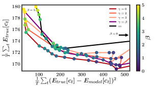
Figure 4a shows result on the industrial benchmark. The $y$-axis in the plot is the average total cost at horizon $T$ obtained by the policy in the ground truth system. The $x$-axis is the average model-bias in the ground truth system according to Eq. (12). Each individual curve in the plot is obtained by fixing $\gamma$ to a specific value (line colour) and then changing $\beta$ (circle colour). The policy that ignores risk ($\beta=\gamma=0$) results in both high model-bias and high cost when evaluated on the ground truth, which indicates overfitting. As $\beta$ increases, the policies put more emphasis on avoiding model-bias, but at the same time the average cost increases. The best tradeoff is obtained by the dark red curve with $\gamma=0$. The risk criterion is then $\beta\sum_{t=1}^{T}\sigma_{q(\mathcal{W})}(\mathbf{E}[c_{t}|\mathcal{W}])$. In this problem, adding aleatoric risk by setting $\gamma>0$ decreases performance. The nn-baseline shows a similar pattern as the BNN+LV approach, but the trade-off between model-bias and cost is worse.

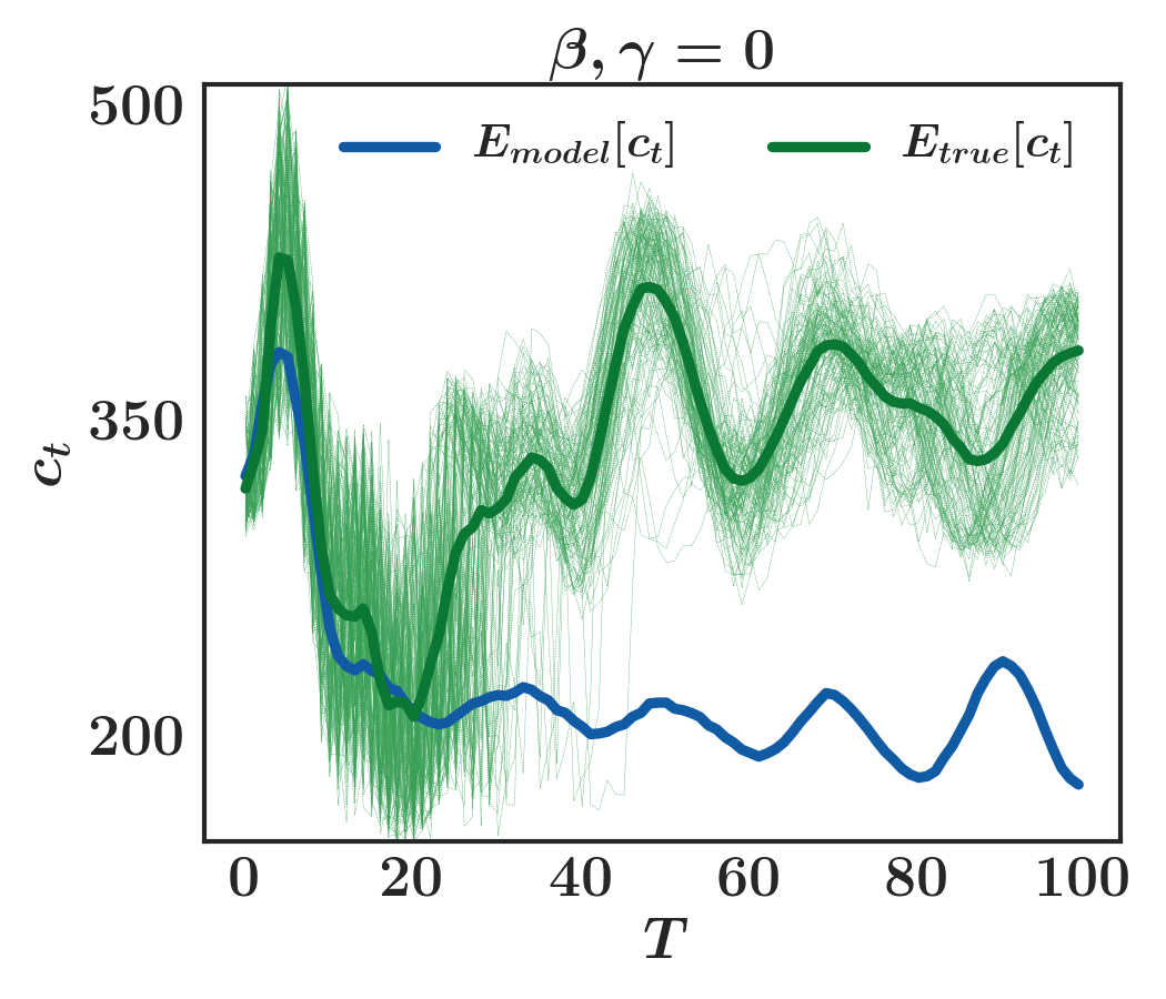
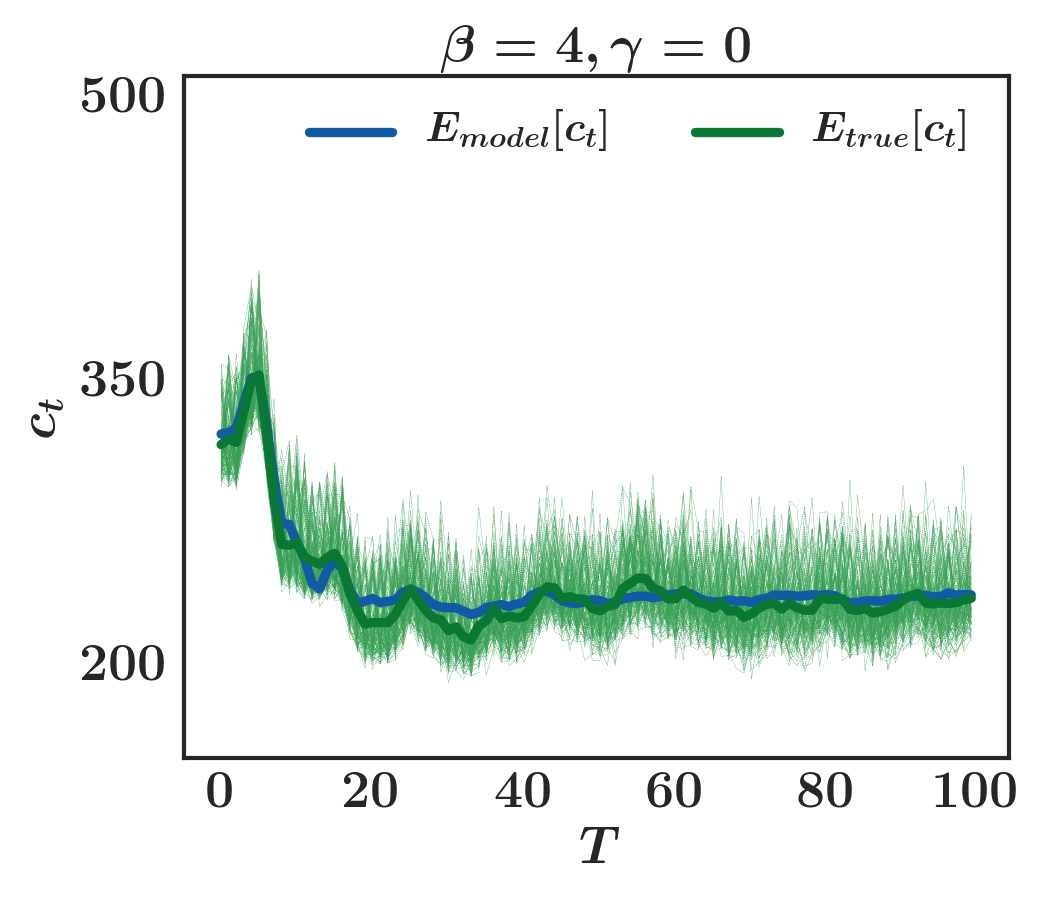
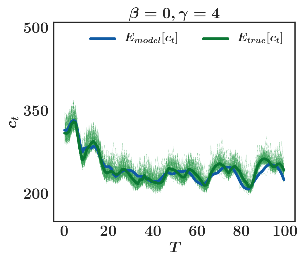
Figure 5 shows roll-outs for three different policies and a fixed initial state $\mathbf{s}_{0}$. Figure 5a shows results for a policy learned with $\gamma=\beta=0$. This policy ignores risk, and as a consequence, the mismatch between predicted performance on the model and on the ground truth increases after $t=20$. This result illustrates how model-bias can lead to policies with high costs at test time. Figure 5b shows results for policy that was trained while penalizing epistemic risk ($\beta=4$, $\gamma=0$). In this case, the average costs under the BNN+LV model and the ground truth are similar, and the overall ground truth cost is lower than in Figure 5a. Finally, Figure 5c shows results for a noise averse policy ($\beta=0$, $\gamma=4$). In this case, the model bias is slightly higher than in the previous figure, but the stochasticity is lower.

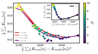
The results for wind turbine simulator can be found in Figure 4b. In this case, the best trade-offs between expected cost and model-bias are obtained by the policies with $\gamma=7.5$. These policies are noise averse and will try to avoid noisy regions in state space. This makes sense because in wind turbines, high noise regions in state space are those where the effect of wind turbulence will have a strong impact on the average cost.

6 Related Work

The distinction between aleatoric and epistemic uncertainty has been recognized in many fields within machine learning, often within the context of specific subfields, models, and objectives. Kendall & Gal (2017) consider a decomposition of uncertainty in the context of computer vision with heteroscedastic Gaussian output noise, while McAllister (2016) consider a decomposition in GPs for model-based RL.

Within reinforcement learning, Bayesian notions of model uncertainty have a long history (Schmidhuber, 1991b, a; Dearden et al., 1999; Still & Precup, 2012; Sun et al., 2011; Maddison et al., 2017). The mentioned works typically consider the online case, where model uncertainty (a.k.a. curiosity) is used to guide exploration, e.g. in Houthooft et al. (2016) the uncertainty of a BNN model is used to guide exploration assuming deterministic dynamics. In contrast, we focus on the batch setting with stochastic dynamics.

Model uncertainty is used in safe or risk-sensitive RL (Mihatsch & Neuneier, 2002; García & Fernández, 2015). In safe RL numerous other approaches exists for safe exploration (Joseph et al., 2013; Hans et al., 2008; Garcia & Fernández, 2012; Berkenkamp et al., 2017). Uncertainties over transition probabilities have been studied in discrete MDPs since a long time (Shapiro & Kleywegt, 2002; Nilim & El Ghaoui, 2005; Bagnell et al., 2001) often with a focus on worst-case avoidance. Our work extends this to continuous state and action space using scalable probabilistic models. Our decomposition enables a practitioner to adjust the optimization criterion to specific decision making,.

Within active learning many approaches exist that follow an information theoretic approach (MacKay, 1992; Hernández-Lobato & Adams, 2015; Guo & Greiner, 2007). To our knowledge, all of these approaches however use deterministic methods (mostly GPs) as model class. Perhaps closest to our work is BALD (Houlsby et al., 2012), however because GPs are used, this approach cannot model problems with complex noise.

7 Conclusion

We have described a decomposition of predictive uncertainty into its epistemic and aleatoric components when working with Bayesian neural networks with latent variables. We have shown how this decomposition of uncertainty can be used for active learning, where it naturally arises from an information-theoretic perspective. We have also used the decomposition to propose a novel risk- sensitive criterion for model-based reinforcement learning which decomposes risk into model-bias and noise aversion components. Our experiments illustrate how the described decomposition of uncertainty is useful for efficient and risk-sensitive learning.

Appendix A Hamiltonian Monte Carlo Solution to Toy Problems

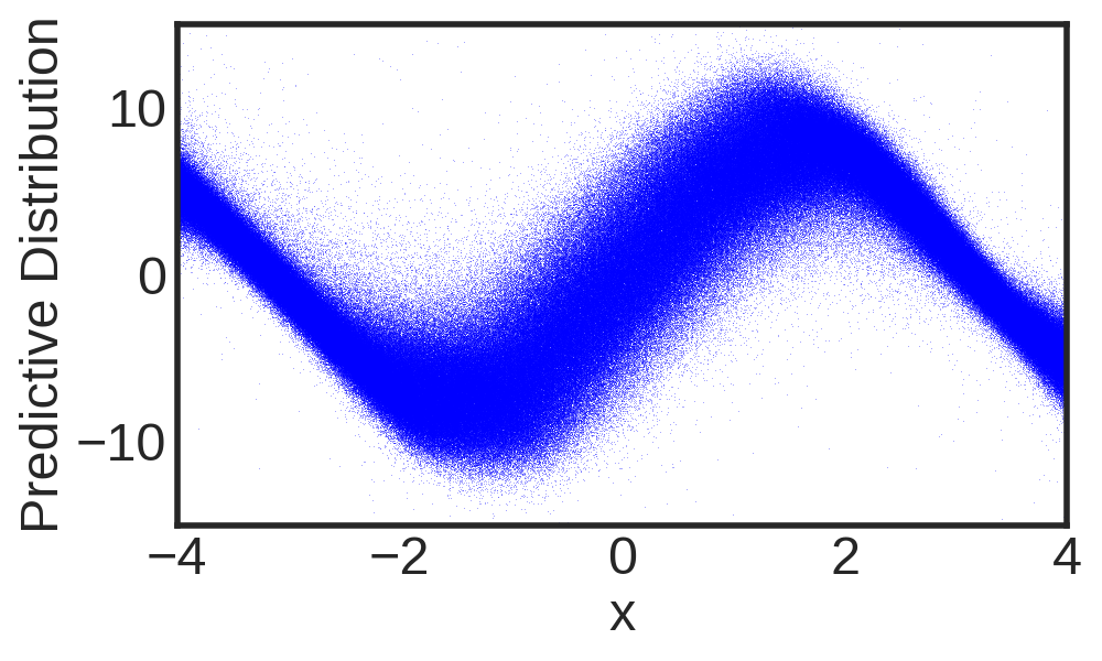
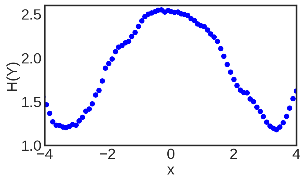
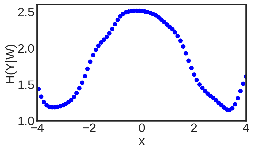
The goal here is to show that the decomposition we obtained in the active learning examples is not a result of our approximation using black-box $\alpha$-divergence minimization but a property of BNN+LV themselves. To that end we will approximate using HMC. After a burn-in of $500,000$ samples we sample from the posterior $200,000$ samples. We thin out 90% by only keeping every tenth sample.

A.1 Heteroscedastic Problem

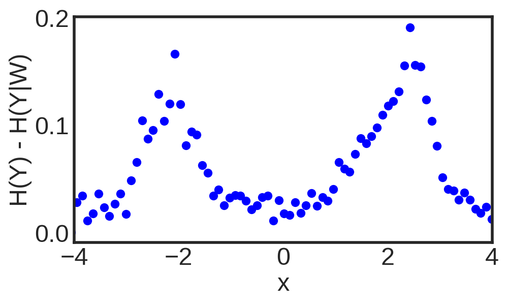
We define the stochastic function $y=7\sin(x)+3|\cos(x/2)|\epsilon$ with $\epsilon\sim\mathcal{N}(0,1)$. The data availability is limited to specific regions of $x$. In particular, we sample 750 values of $x$ from a mixture of three Gaussians with mean parameters $\{\mu_{1}=-4,\mu_{2}=0,\mu_{3}=4\}$, variance parameters $\{\sigma_{1}=\frac{2}{5},\sigma_{2}=0.9,\sigma_{3}=\frac{2}{5}\}$ and with each Gaussian component having weight equal to $1/3$ in the mixture. Figure 6a shows the raw data. We have lots of points at both borders of the $x$ axis and in the center, but little data available in between.

(a)

(b)

(c)

(d)

(e)

(f)

Figure 6: HMC results of active learning example using heteroscedastic data. LABEL:sub@fig:hmcrd: Raw data. LABEL:sub@fig:hmcdd: Density of $x$ in raw data. LABEL:sub@fig:hmcpd: Predictive distribution: $p(y|x)$ of BNN using HMC. LABEL:sub@fig:hmch: Entropy estimate $\text{H}(y|x)$ of predictive distribution for each $x$. LABEL:sub@fig:hmchgw: Conditional Entropy estimate $\mathbf{E}_{\mathcal{W}}\text{H}(y|x,\mathcal{W})$ of predictive distribution for each $x$. LABEL:sub@fig:hmcob: Estimate of reduction in entropy for each $x$.

A.2 Bimodal Problem

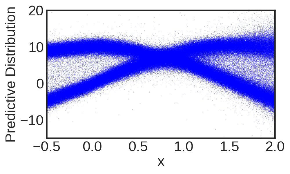
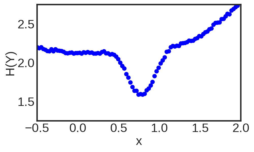
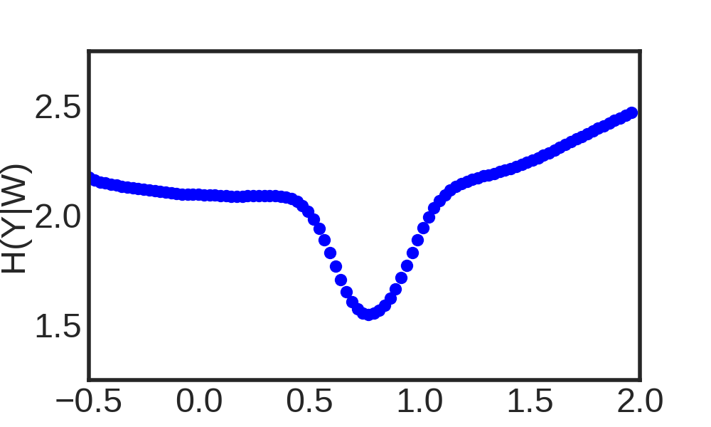
We consider a toy problem given by a regression task with bimodal data. We define $x\in[-0.5,2]$ and $y=10\sin(x)+\epsilon$ with probability $0.5$ and $y=10\cos(x)+\epsilon$, otherwise, where $\epsilon\sim\mathcal{N}(0,1)$ and $\epsilon$ is independent of $x$. The data availability is not uniform in $x$. In particular we sample 750 values of $x$ from an exponential distribution with $\lambda=2$

(a)

(b)

(c)

(d)

(e)

(f)

Figure 7: HMC results of active learning example using bimodal data. LABEL:sub@fig:hmcbrd: Raw data. LABEL:sub@fig:hmcbdd: Density of $x$ in raw data. LABEL:sub@fig:hmcbpd: Predictive distribution: $p(y|x)$ of BNN using Hamilton monte carlo. LABEL:sub@fig:hmcbh: Entropy estimate $\text{H}(y|x)$ of predictive distribution for each $x$. LABEL:sub@fig:hmcbhgw: Conditional Entropy estimate $\mathbf{E}_{\mathcal{W}}\text{H}(y|x,\mathcal{W})$ of predictive distribution for each $x$. LABEL:sub@fig:hmcbob: Estimate of reduction in entropy for each $x$.

Appendix B Solutions to Toy Problems for different values of $\alpha$

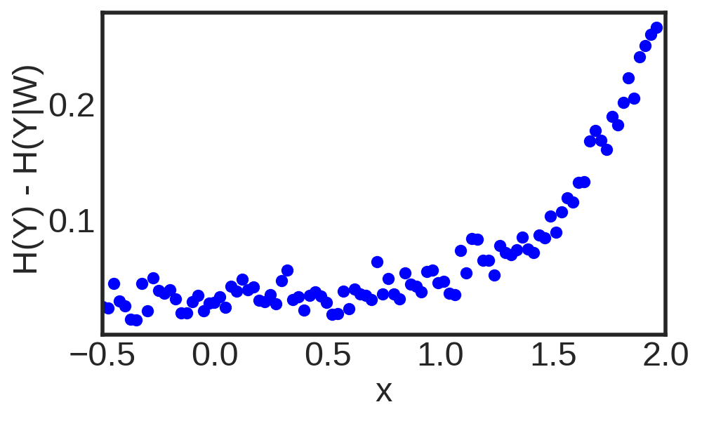
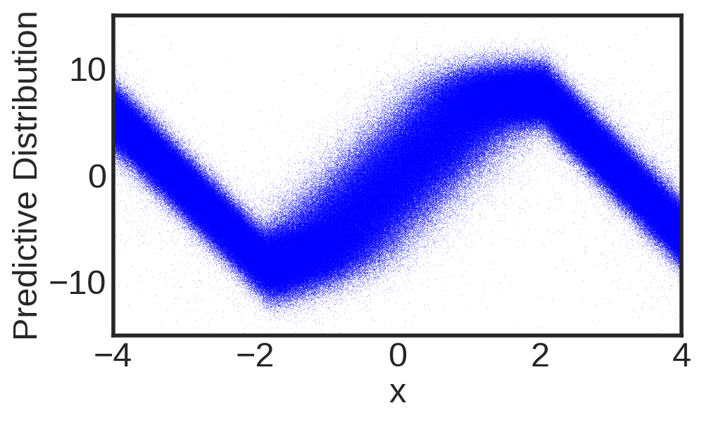
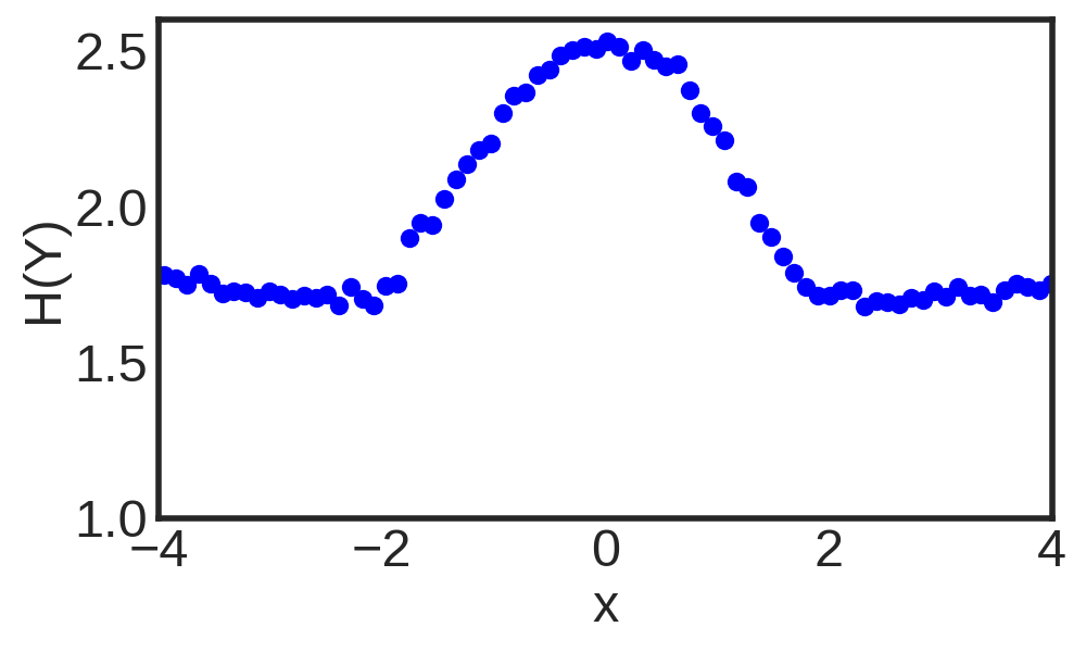
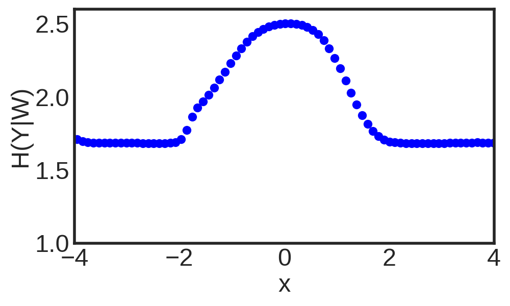
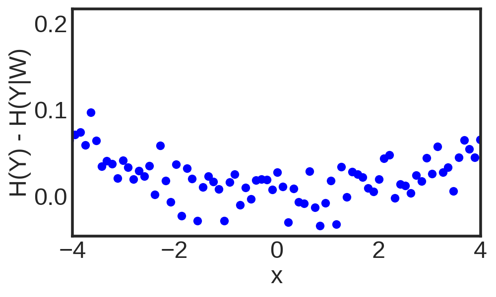
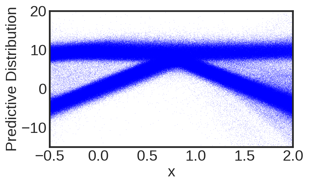
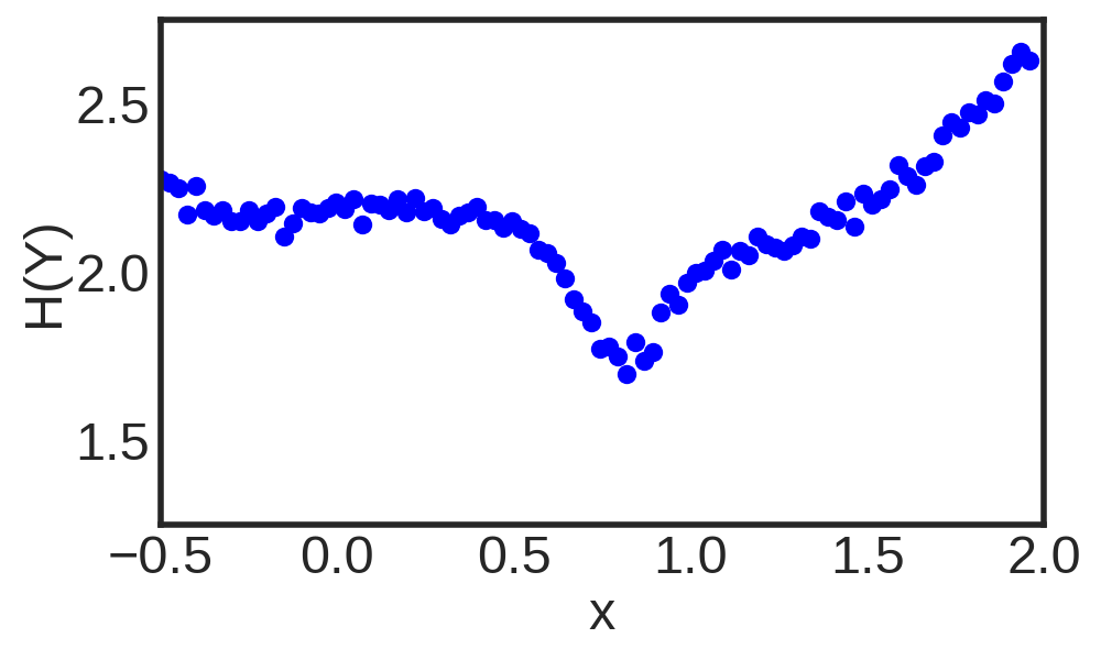
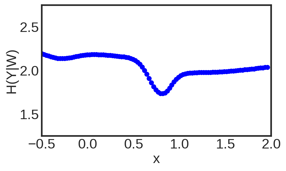
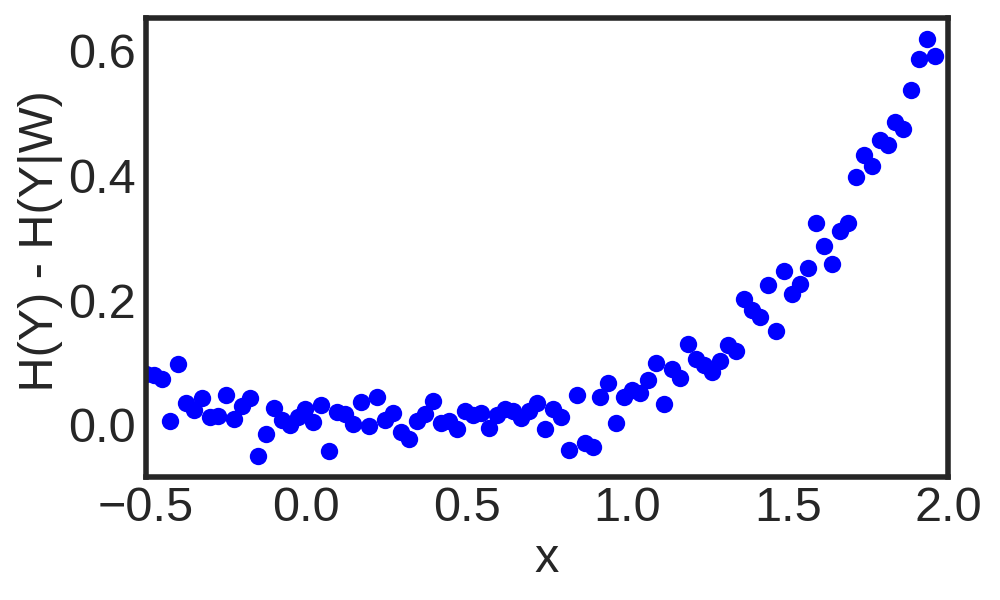
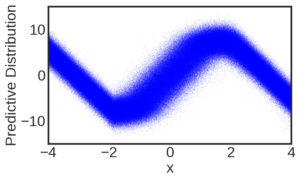
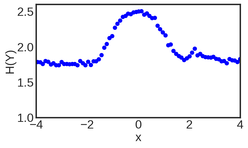
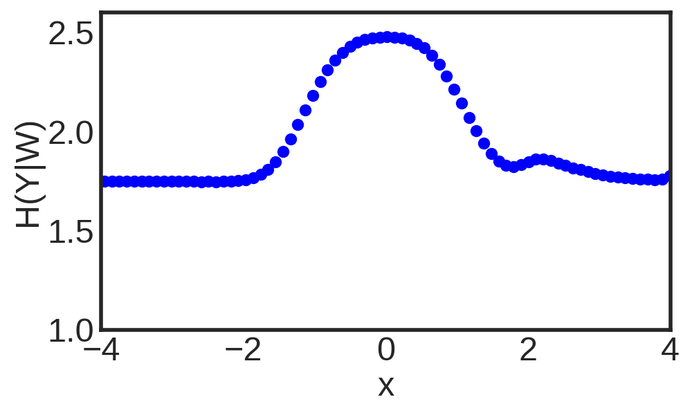
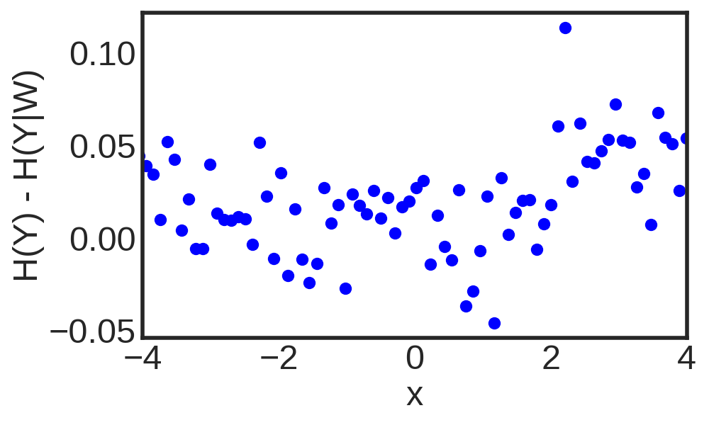
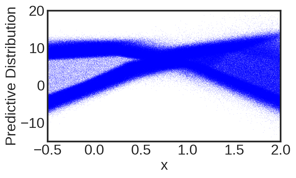
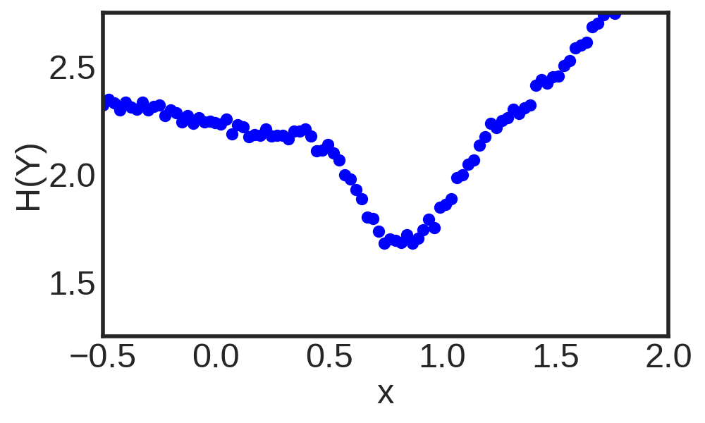
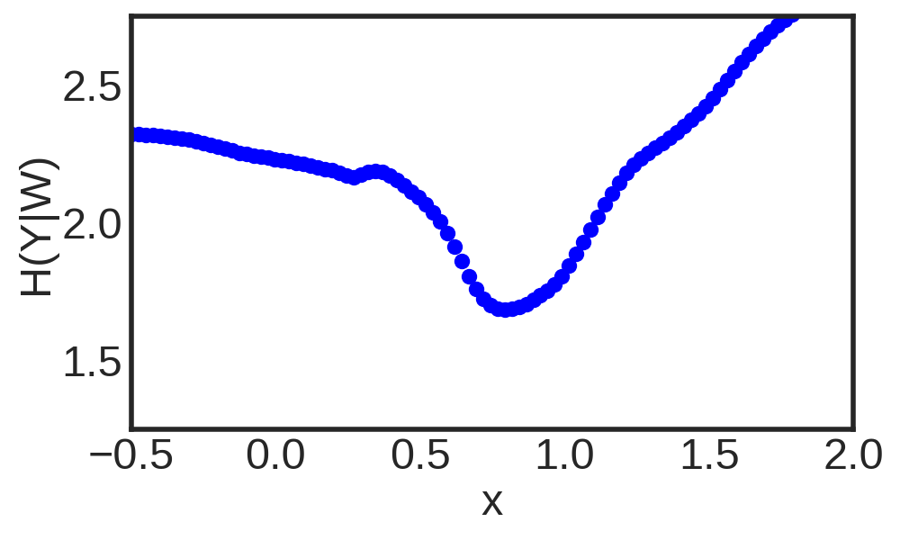
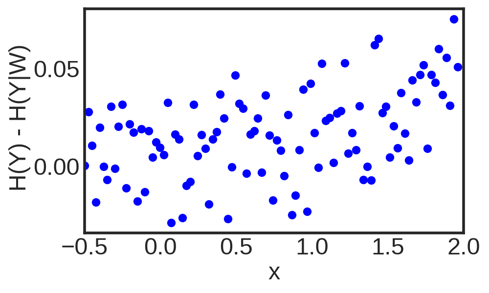
In the main document we pointed out that the decomposition of uncertainty does not work as good with other values of $\alpha$. We will see in the following, that lower values of $\alpha$ will put more and more emphasis on the latent variable $z$. We observe that the epistemic uncertainty will vanish as the $\alpha$-divergence minimization approaches variational Bayes.

B.1 $\alpha=0.5$

(a)

(b)

(c)

(d)

(e)

(f)

Figure 8: Active learning example using heteroscedastic data using a BNN optimized with bb-$\alpha$ with $\alpha=0.5$. LABEL:sub@fig:a05rd: Raw data. LABEL:sub@fig:a05dd: Density of $x$ in raw data. LABEL:sub@fig:a05pd: Predictive distribution: $p(y|x)$ of BNN. LABEL:sub@fig:a05h: Entropy estimate $\text{H}(y|x)$ of predictive distribution for each $x$. LABEL:sub@fig:a05hgw: Conditional Entropy estimate $\mathbf{E}_{\mathcal{W}}\text{H}(y|x,\mathcal{W})$ of predictive distribution for each $x$. LABEL:sub@fig:a05ob: Estimate of reduction in entropy for each $x$.

(a)

(b)

(c)

(d)

(e)

(f)

Figure 9: Active learning example using bimodal data using a BNN optimized with bb-$\alpha$ with $\alpha=0.5$. LABEL:sub@fig:a05brd: Raw data. LABEL:sub@fig:a05bdd: Density of $x$ in raw data. LABEL:sub@fig:a05bpd: Predictive distribution: $p(y|x)$ of BNN. LABEL:sub@fig:a05bh: Entropy estimate $\text{H}(y|x)$ of predictive distribution for each $x$. LABEL:sub@fig:a05bhgw: Conditional Entropy estimate $\mathbf{E}_{\mathcal{W}}\text{H}(y|x,\mathcal{W})$ of predictive distribution for each $x$. LABEL:sub@fig:a05bob: Estimate of reduction in entropy for each $x$.

B.2 $VB$ solutions to Toy Problems

We approximate the method variational Bayes by setting $\alpha$ to $10^{-6}$.

(a)

(b)

(c)

(d)

(e)

(f)

Figure 10: Active learning example using heteroscedastic data using a BNN optimized by variational Bayes. LABEL:sub@fig:a00rd: Raw data. LABEL:sub@fig:a00dd: Density of $x$ in raw data. LABEL:sub@fig:a00pd: Predictive distribution: $p(y|x)$ of BNN. LABEL:sub@fig:a00h: Entropy estimate $\text{H}(y|x)$ of predictive distribution for each $x$. LABEL:sub@fig:a00hgw: Conditional Entropy estimate $\mathbf{E}_{\mathcal{W}}\text{H}(y|x,\mathcal{W})$ of predictive distribution for each $x$. LABEL:sub@fig:a00ob: Estimate of reduction in entropy for each $x$.

(a)

(b)

(c)

(d)

(e)

(f)

Figure 11: Active learning example using bimodal data using a BNN optimized by variational Bayes. LABEL:sub@fig:a00brd: Raw data. LABEL:sub@fig:a00bdd: Density of $x$ in raw data. LABEL:sub@fig:a00bpd: Predictive distribution: $p(y|x)$ of BNN. LABEL:sub@fig:a00bh: Entropy estimate $\text{H}(y|x)$ of predictive distribution for each $x$. LABEL:sub@fig:a00bhgw: Conditional Entropy estimate $\mathbf{E}_{\mathcal{W}}\text{H}(y|x,\mathcal{W})$ of predictive distribution for each $x$. LABEL:sub@fig:a00bob: Estimate of reduction in entropy for each $x$.

Appendix C Experiments Specification

C.1 Active Learning

All models start with the available described in the respective paragraphs. We train for $5000$ epochs a BNN+LV with two-hidden layer and $20$ hidden units per layer. We use Adam as optimizer with a learning rate of $0.001$. For Gaussian processes(GPs) we use the standard RBF kernel using the python GPy implementation. For the entropy estimation we use a nearest-neighbor approach as explained in the main document with $k=25$ and $500$ samples of $q(W)$ and $500$ samples of $p(z)$.

For active learning we evaluate performance using a held-out test set of size $500$ for the bimodal and heteroscedastic problem and $2500$ for the wet-chicken problem. The test data is sampled uniformly in state (and action) space. In each of the $n=150$ iterations we sample a pool set of size $50$ uniformly in input space. In each iteration a method can decide to include $5$ data points into the training set. After that, the models are re-trained (from scratch) and the performance is evaluated on the test set.

C.2 Wet-chicken

We use the continuous two-dimensional version of the problem. A canoeist is paddling on a two-dimensional river. The canoeist’s position at time $t$ is $(x_{t},y_{t})$. The river has width $w=5$ and length $l=5$ with a waterfall at the end, that is, at $y_{t}=l$. The canoeist wants to move as close to the waterfall as possible because at time $t$ he gets reward $r_{t}=-(l-y_{t})$. However, going beyond the waterfall boundary makes the canoeist fall down, having to start back again at the origin $(0,0)$. At time $t$ the canoeist can choose an action $(a_{t,x},a_{t,y})\in[-1,1]^{2}$ that represents the direction and magnitude of his paddling. The river dynamics have stochastic turbulences $s_{t}$ and drift $v_{t}$ that depend on the canoeist’s position on the $x$ axis. The larger $x_{t}$, the larger the drift and the smaller $x_{t}$, the larger the turbulences.

The underlying dynamics are given by the following system of equations. The drift and the turbulence magnitude are given by $v_{t}=3x_{t}w^{-1}$ and $s_{t}=3.5-v_{t}$, respectively. The new location $(x_{t+1},y_{t+1})$ is given by the current location $(x_{t},y_{t})$ and current action $(a_{t,x},a_{t,y})$ using

$$x_{t+1} =\begin{cases}0&\text{if }\quad x_{t}+a_{t,x}<0\\ 0&\text{if }\quad\hat{y}_{t+1}>l\\ w&\text{if }\quad x_{t}+a_{t,x}>w\\ x_{t}+a_{t,x}&\text{otherwise}\end{cases}\,, y_{t+1} =\begin{cases}0&\text{if }\quad\hat{y}_{t+1}<0\\ 0&\text{if }\quad\hat{y}_{t+1}>l\\ \hat{y}_{t+1}&\text{otherwise}\end{cases}\,,$$ (14)

where $\hat{y}_{t+1}=y_{t}+(a_{t,y}-1)+v_{t}+s_{t}\tau_{t}$ and $\tau_{t}\sim\text{Unif}([-1,1])$ is a random variable that represents the current turbulence. As the canoeist moves closer to the waterfall, the distribution for the next state becomes increasingly bi-modal because when he is close to the waterfall, the change in the current location can be large if the canoeist falls down the waterfall and starts again at $(0,0)$. The distribution may also be truncated uniform for states close to the borders. Furthermore the system has heteroscedastic noise, the smaller the value of $x_{t}$ the higher the noise variance.

C.3 Reinforcement Learning

C.3.1 Industrial benchmark

Policies in the industrial benchmark specify changes $\Delta_{v}$, $\Delta_{g}$ and $\Delta_{s}$ in three steering variables $v$ (velocity), $g$ (gain) and $s$ (shift) as a function of $\mathbf{s}_{t}$. In the behavior policy these changes are stochastic and sampled according to

$$\Delta_{v} =\left\{\begin{array}[]{@{}ll@{}}z_{v}\,,&\text{if}\,\,v(t)<40\\ -z_{v}\,,&\text{if}\,\,v(t)>60\\ u_{v}\,,&\text{otherwise}\end{array}\right.$$ (18)

$$\Delta_{g} =\left\{\begin{array}[]{@{}ll@{}}z_{g}\,,&\text{if}\,\,g(t)<40\\ -z_{g}\,,&\text{if}\,\,g(t)>60\\ u_{g}\,,&\text{otherwise}\end{array}\right.$$ (22)

$$\Delta_{s} =u_{s}\,,$$ (23)

where $z_{v},z_{g}\sim\mathcal{N}(0.5,\frac{1}{\sqrt{3}})$ and $u_{v},u_{g},u_{s}\sim\mathcal{U}(-1,1)$. The velocity $v(t)$ and gain $g(t)$ can take values in $[0,100]$. Therefore, the data collection policy will try to keep these values only in the medium range given by the interval $[40,60]$. Because of this, large parts of the state space will be unobserved. After collecting the data, the $30,000$ state transitions are used to train a BNN with latent variables with the same hyperparameters as in (Depeweg et al., 2016). Finally, we train different policies using the Monte Carlo approximation and we set the horizon of $T=100$ steps, with $M=50$ and $N=25$ and a minibatch size of $1$ for $750$ epochs. The total training time on a single CPU is around $18$ hours.

C.3.2 Wind Turbine Simulator

In this problem we observe the turbine state $s(t)$, with features such as current wind speed and currently produced power. Our actions $a(t)$ adjust the turbine’s behavior, with known upper and lower bounds. The goal is to maximize energy output over a $T$-step horizon.

We are given a batch of around 5,000 state transitions generated by a behavior policy $\pi_{b}$. The policy does limited exploration around the neutral action $a(t)=0$.

The system is expected to be highly stochastic due to the unpredictability of future wind dynamics. Furthermore the dimensionality of state observation is much higher than the action dimensionality, so, with the limited dataset that we have, we expect it to be very challenging to accurately learn the influence of the action on the reward.

First we train a BNN with two hidden layer and 50 hidden units per layer on the available batch using $\alpha$-divergence minimization with $\alpha=1.0$. In the second step, using the model, we train a policy with 20 hidden units on each of the two layers in the usual way, using the Monte Carlo estimate. The total training time on a single CPU is around $8$ hours.

References

- Bagnell et al. (2001) Bagnell, J. A., Ng, A. Y., and Schneider, J. G. Solving uncertain markov decision processes. 2001.
- Beirlant et al. (1997) Beirlant, J., Dudewicz, E. J., Györfi, L., and Van der Meulen, E. C. Nonparametric entropy estimation: An overview. International Journal of Mathematical and Statistical Sciences, 6(1):17–39, 1997.
- Berkenkamp et al. (2017) Berkenkamp, F., Turchetta, M., Schoellig, A. P., and Krause, A. Safe model-based reinforcement learning with stability guarantees. In Advances in Neural Information Processing Systems (NIPS), pp. 908–918, 2017.
- Blundell et al. (2015) Blundell, C., Cornebise, J., Kavukcuoglu, K., and Wierstra, D. Weight uncertainty in neural networks. In International Conference on Machine Learning (ICML), pp. 1613–1622, 2015.
- Dearden et al. (1999) Dearden, R., Friedman, N., and Andre, D. Model based bayesian exploration. In Proceedings of the Fifteenth conference on Uncertainty in artificial intelligence (UAI), pp. 150–159, 1999.
- Deisenroth & Rasmussen (2011) Deisenroth, M. and Rasmussen, C. E. Pilco: A model-based and data-efficient approach to policy search. In Proceedings of the 28th International Conference on machine learning (ICML-11), pp. 465–472, 2011.
- Depeweg et al. (2016) Depeweg, S., Hernández-Lobato, J. M., Doshi-Velez, F., and Udluft, S. Learning and policy search in stochastic dynamical systems with bayesian neural networks. International Conference on Learning Representations (ICLR), 2016.
- Der Kiureghian & Ditlevsen (2009) Der Kiureghian, A. and Ditlevsen, O. Aleatory or epistemic? does it matter? Structural Safety, 31(2):105–112, 2009.
- Gal (2016) Gal, Y. Uncertainty in deep learning. PhD thesis, University of Cambridge, 2016.
- Gao et al. (2016) Gao, W., Oh, S., and Viswanath, P. Breaking the bandwidth barrier: Geometrical adaptive entropy estimation. In Advances in Neural Information Processing Systems (NIPS), pp. 2460–2468, 2016.
- Garcia & Fernández (2012) Garcia, J. and Fernández, F. Safe exploration of state and action spaces in reinforcement learning. Journal of Artificial Intelligence Research, 45:515–564, 2012.
- García & Fernández (2015) García, J. and Fernández, F. A comprehensive survey on safe reinforcement learning. The Journal of Machine Learning Research, 16(1):1437–1480, 2015.
- Guo & Greiner (2007) Guo, Y. and Greiner, R. Optimistic active-learning using mutual information. In International Joint Conference on Artificial Intelligence (IJCAI), pp. 823–829, 2007.
- Hans & Udluft (2009) Hans, A. and Udluft, S. Efficient uncertainty propagation for reinforcement learning with limited data. In International Conference on Artificial Neural Networks (ICANN), pp. 70–79. 2009.
- Hans et al. (2008) Hans, A., Schneegaß, D., Schäfer, A. M., and Udluft, S. Safe exploration for reinforcement learning. In ESANN, pp. 143–148, 2008.
- Hein et al. (2017) Hein, D., Depeweg, S., Tokic, M., Udluft, S., Hentschel, A., Runkler, T. A., and Sterzing, V. A benchmark environment motivated by industrial control problems. IEEE Symposium on Computational Intelligence (IEEE SSCI), 2017.
- Hernández-Lobato & Adams (2015) Hernández-Lobato, J. M. and Adams, R. Probabilistic backpropagation for scalable learning of bayesian neural networks. In International Conference on Machine Learning (ICML), pp. 1861–1869, 2015.
- Hernández-Lobato et al. (2016) Hernández-Lobato, J. M., Li, Y., Rowland, M., Hernández-Lobato, D., Bui, T., and Turner, R. E. Black-box -divergence minimization. In International Conference on Machine Learning (ICML), pp. 1861–1869, 2016.
- Houlsby et al. (2012) Houlsby, N., Huszar, F., Ghahramani, Z., and Hernández-Lobato, J. M. Collaborative gaussian processes for preference learning. In Advances in Neural Information Processing Systems (NIPS), pp. 2096–2104, 2012.
- Houthooft et al. (2016) Houthooft, R., Chen, X., Duan, Y., Schulman, J., De Turck, F., and Abbeel, P. VIME: Variational information maximizing exploration. In Advances in Neural Information Processing Systems (NIPS), pp. 1109–1117, 2016.
- Joseph et al. (2013) Joseph, J., Geramifard, A., Roberts, J. W., How, J. P., and Roy, N. Reinforcement learning with misspecified model classes. In International Conference on Robotics and Automation (ICRA), pp. 939–946, 2013.
- Kendall & Gal (2017) Kendall, A. and Gal, Y. What uncertainties do we need in bayesian deep learning for computer vision? In Advances in Neural Information Processing Systems (NIPS), pp. 5580–5590, 2017.
- Kozachenko & Leonenko (1987) Kozachenko, L. and Leonenko, N. N. Sample estimate of the entropy of a random vector. Problemy Peredachi Informatsii, 23(2):9–16, 1987.
- Kraskov et al. (2004) Kraskov, A., Stögbauer, H., and Grassberger, P. Estimating mutual information. Physical review E, 69(6):066138, 2004.
- Lange et al. (2012) Lange, S., Gabel, T., and Riedmiller, M. Batch reinforcement learning. In Reinforcement learning, pp. 45–73. Springer, 2012.
- Larsen & Hansen (2007) Larsen, T. J. and Hansen, A. M. How 2 hawc2, the user’s manual. Technical report, Risø National Laboratory, 2007.
- Larsen et al. (2015) Larsen, T. J., Larsen, G., Madsen, H. A., Thomsen, K., and Pedersen, S. M. Comparison of measured and simulated loads for the siemens swt2.3 operating in wake conditions at the lillgrund wind farm using hawc2 and the dynamic wake meander model. EWEA offshore 2015, 2015.
- Le et al. (2005) Le, Q. V., Smola, A. J., and Canu, S. Heteroscedastic gaussian process regression. In International Conference on Machine Learning (ICML), pp. 489–496, 2005.
- MacKay (1992) MacKay, D. J. Information-based objective functions for active data selection. Neural computation, 4(4):590–604, 1992.
- Maddison et al. (2017) Maddison, C. J., Lawson, D., Tucker, G., Heess, N., Doucet, A., Mnih, A., and Teh, Y. W. Particle value functions. arXiv preprint arXiv:1703.05820, 2017.
- McAllister (2016) McAllister, R. Bayesian Learning for Data-Efficient Control. PhD thesis, King’s College, 2016.
- Mihatsch & Neuneier (2002) Mihatsch, O. and Neuneier, R. Risk-sensitive reinforcement learning. Machine learning, 49(2-3):267–290, 2002.
- Nilim & El Ghaoui (2005) Nilim, A. and El Ghaoui, L. Robust control of markov decision processes with uncertain transition matrices. Operations Research, 53(5):780–798, 2005.
- Schmidhuber (1991a) Schmidhuber, J. Curious model-building control systems. In IEEE International Joint Conference on Neural Networks, pp. 1458–1463, 1991a.
- Schmidhuber (1991b) Schmidhuber, J. A possibility for implementing curiosity and boredom in model-building neural controllers. In From animals to animats: Proceedings of the first international conference on simulation of adaptive behavior, pp. 15–21. Citeseer, 1991b.
- Settles (2012) Settles, B. Active learning. Synthesis Lectures on Artificial Intelligence and Machine Learning, 6(1):1–114, 2012.
- Shapiro & Kleywegt (2002) Shapiro, A. and Kleywegt, A. Minimax analysis of stochastic problems. Optimization Methods and Software, 17(3):523–542, 2002.
- Still & Precup (2012) Still, S. and Precup, D. An information-theoretic approach to curiosity-driven reinforcement learning. Theory in Biosciences, pp. 139–148, 2012.
- Sun et al. (2011) Sun, Y., Gomez, F., and Schmidhuber, J. Planning to be surprised: Optimal bayesian exploration in dynamic environments. In International Conference on Artificial General Intelligence, pp. 41–51, 2011.