Informational Neurobayesian Approach to Neural Networks Training. Opportunities and Prospects

Abstract

A study of the classification problem in context of information theory is presented in the paper. Current research in that field is focused on optimisation and bayesian approach. Although that gives satisfying results, they require a vast amount of data and computations to train on. Authors propose a new concept, named Informational Neurobayesian Approach (INA), which allows to solve the same problems, but requires significantly less training data as well as computational power. Experiments were conducted to compare its performance with the traditional one’s and the results showed that capacity of the INA is quite promising.

Keywords: Informational Neurobayesian Approach, text recognition, information quantity, classification, Sequence to Sequence model, Neurobayesian Approach, Gradient Descent, one-shot learning, information emergence, large neural networks, information neural models.

1 Introduction

The classification problem nowadays is usually solved by complex analytical algorithms requiring plenty of data. Another field of research is neurobayesian approach, which proposes optimisation based on Bayes rule with some tricks to cope with functions complexity and make them well-defined. The authors introduce a method based on the same concepts but they also take into consideration the informational side of the data - namely its meaning.

The problem of determining the quantity of information until recently was based on Hartley and Shennon approaches. The first one represents just the quantity of information, the second is its generalisation which takes into account different probabilities for classes. Another fundamental concept is Harkevich formula which measures the informational value of event or message as the logarithm of ratio of probability of a class after and before the event. The System Theory of Information (STI) proposed by Lucenko merges these concepts, taking each formula with corresponding power, which illustrates the emergence of classes and features. The main idea of the article is to develop a method, that allows to calculate weight coefficients of artificial neural network’s synapses. We propose to move from uninterpreted weights (trial and error method) to the weight representing the amount of information that is contained in the feature regarding a possible consequence. Thus, a neural network is considered as a self-training system of transforming the input data into the amount of information about the possible consequences.The proposed approach allows to train big neuromodels with billions of neurons on ordinary CPUs.

2 Classical Gradient Descent

2.1 Description

Gradient Descent is a widely used approach to solve optimisation problems which are too complex to find solution analytically. As the approach proposed in the paper is applied in the context of neural networks, we will briefly show the usage of gradient descent for their training.

The problem is formulated in the following way: model’s performance is measured by the error function, which depends on $n$ neurons and $m$ observations. So, $n$ weights are to be optimised to achieve the minimum of error function. The gradient descent principle is to push the weights towards the direction opposite to the error function’s gradient (all weights are changed simultaneously).

2.2 Formulae

$$\nabla Q(w_{0},w_{1},...,w_{n})=\Bigg{[}\frac{\delta Q}{\delta w_{0}},...,\frac{\delta Q}{\delta w_{n}}\Bigg{]}$$

So, on each iteration the weights are updated according the following rule:

$$w_{i}=w_{i}-\mu\frac{\delta Q}{\delta w_{i}},$$

where $\mu$ is an exogenous parameter, which determines the learning rate. The most popular type of error functions is sum of squares, so the aim is to minimise the expression:

$$Q(w_{0},w_{1},...,w_{n})=\frac{1}{2}\sum^{m}_{j=1}(y_{j}-f(x_{0}^{j},x_{1}^{j},...,x_{n}^{j}))^{2},$$

where $f(x_{0}^{j},x_{1}^{j},...,x_{n}^{j})=\sum^{n}_{i=1}w_{i}x_{i}^{j}$ is a linear function, giving the values on the output of the neuron and depending on the weights of the input vector (instead of linear various functions can be used, e.g. tanh, sigmoid, softmax, the general principle remains the same). The derivative by each weight will be equal:

$$\frac{\delta Q(\cdot)}{\delta w_{i}}=\frac{1}{2}\sum^{m}_{j=1}\frac{\delta}{\delta w_{i}}(y_{j}-\sum^{n}_{i=1}w_{i}x_{i}^{j})^{2}=$$

$$=\sum^{m}_{j=1}(y_{j}-\sum^{n}_{i=1}w_{i}x_{i}^{j})(-x_{i}^{j})$$

So, the formula for weights updating is:

$$w_{i}=w_{i}+\mu x_{i}^{j}\sum^{m}_{j=1}(y_{j}-\sum^{n}_{i=1}w_{i}x_{i}^{j})$$

Iterations are performed until the weight’s changes are more than some exogenous determined parameter.

2.3 Advantages and disadvantages

The approach performs well for a very narrow class of problems, though it has advanced modifications like Adagrad, Adam, and Gradient Boosting which show outstanding results although require considerable computational power.

2.4 Computational Complexity

Algorithm’s complexity for the described case is $O(n^{2})$ as on each iteration the sum of $n$ terms is computed $n$ times. The complexity is linear relative to input data size.

3 Neurobayesian Approach

3.1 Description

The bayesian approach means designing the forecast of distribution of variables and then updating it based on new knowledge about an object. Bayesian framework in comparison with traditional (frequentist) one considers all data random, makes great use of Bayes theorem and instead of ML-estimates maximise posterior probability. Though it works with any amount of data, even small,the more information about the object is obtained, the more precise the final knowledge will be (the Bayesian updating can be applied iteratively as new data becomes available).

The problem is formulated as follows: let $p(X,T,W)$ be a joint distribution of hidden variables $T$, observed variables $X$ and decision rule parameters $W$. If training data is $(X_{tr},T_{tr})$, then posterior distribution of W is

$$p(W|T_{tr},X_{tr})=\frac{p(T_{tr},X_{tr}|W)p(W)}{\int p(T_{tr},X_{tr}|W)p(W)dW}$$

Analytical approach to that expression is to make use of delta-method and maximise likelihood function. But the bayesian approach proposes a less straightforward, yet fruitful step - to regularise ML estimate using prior distribution. It helps to cope with overfitting and gives a more thorough picture of hidden variables and also allows to learn from incomplete data. But the main advantage is the possibility of the algorithm to obtain high accuracy results with big data. Application of bayesian approach to neural networks is based on cross-entropy error function minimisation with updating of the weights using existing data.

3.2 Formulae

In practice the optimisation procedure goes in the following way[2][Vetrov D., 2017]. If only $X_{tr}$ is known, $T$ is a hidden variables vector, $p(X),q(T)$ are their density functions respectively, and $W$ is to be determined, then:

$$W_{*}=\arg\max p(W|X_{tr})=\arg\max\log p(W|X_{tr})=$$

$$=\arg\max(\log p(X_{tr}|W)+\log p(W))=$$

$$=\arg\max\Big{(}\log\int p(X_{tr},T|W)dT+\log p(W)\Big{)}$$

The problem is that the first term is not concave. To cope with that a trick is introduced:

$$\log p(X_{tr}|W)=\int q(T)\log p(X_{tr}|W)dT=$$

$$=\int q(T)\log\frac{p(X_{tr},T|W)}{p(T|X_{tr},W)}dT=$$

$$=\int q(T)\log\frac{p(X_{tr},T|W)q(T)}{p(T|X_{tr},W)q(T)}dT=$$

$$=\int q(T)\log\frac{p(X_{tr},T|W)}{q(T)}dT+\int q(T)\log\frac{q(T)}{p(T|X_{tr},W)}dT=$$

$$\mathcal{L}(q,W)+KL(q(T)||p(T|X_{tr},W))$$

where $KL(q||p)$ is Kullback-Leibler divergence, which can be interpreted as distance between distribution and is always non-negative. So we can iteratively maximize $\mathcal{L}(q,W)$ instead of original expression. Procedure is called EM-Algorithm and consists of two steps:

1. E-step $\mathcal{L}(q,W_{t-1})\rightarrow\max_{q}$ - corresponds to KL-divergence minimization.

   $$q_{t}(T)=\arg\min_{q}KL(q(T)||p(T|X_{tr},W_{t-1}))=p(T|X_{tr},W_{t-1})$$

2. M-step $\mathcal{L}(q,W_{t-1})\rightarrow\max_{W}.$

   $$W_{t}=\arg\max_{w}\mathcal{L}(q,W_{t-1})=$$

   $$=\arg\max_{w}\int q_{t}(T)\log\frac{p(X_{tr},T|W)}{q_{t}(T)}dT=$$

   $$=\arg\max_{w}\int q_{t}(T)\log p(X_{tr},T|W)dT,$$

   which is a concave function, so the maximisation is legal.

The procedure is repeated until convergence.

3.3 Advantages and disadvantages

The main advantage of the approach is its scalability to large datasets, and less complexity in comparison with analytical optimisation solutions, which are quadratic over data size $O(n^{2})$, while EM algorithm is linear on data $O(n)$ and weight vector’s dimensions. The approach allows to combine models, trained on different data (for same consequences), and thus achieve better results. The drawback is that the approach does not take into consideration the data’s structure, its intrinsic features, which can be exploited to build more realistic a priori distributions and achieve better performance. Since 2012, a number of studies were published, in which a new mathematical apparatus that allows to scale Bayesian methods to big data is proposed. At the heart of it lies an interesting idea. First, the problem of Bayesian inference (that is, the process of application of the Bayes theorem to data) was formulated as an optimization problem, and then modern techniques of stochastic optimization were applied to it, which made it possible to solve extremely large optimization problems approximately. This allowed Bayesian methods to enter the field of neural networks.Over the past 5 years, a whole class of Neurobayes models, that can solve a wider range of problems than conventional deep-seated neural networks, has been developed.

4 Informational Neurobayesian Approach

4.1 Theoretical background

Some facts from the information theory are required for understanding this article. At first, the number of characters that can be obtained using the alphabet consisting of n symbols is $N=m^{n},$ where $n$ is the number of characters in the message. To avoid exponential dependency, it was proposed by Hartly to represent the quantity of information as a logarithm of number of all possible sequences:

$$I=\log N=\log m^{n}=n\log m$$

Let there be $k$ characters, each has $m$ features and $p_{i}$ is a probability to get each feature. Shannon proposed a proportion for determining the average quantity of information in a message with random probabilities of character’s values:

$$I=-k\sum_{i=1}^{m}p_{i}\log p_{i}$$

The more uncertain is the consequence, the more information can be obtained from receiving the information about the consequence.To measure the uncertainty we use entropy, which is the average quantity of information per character.

$$H=\frac{I}{k}=-\sum_{i=1}^{m}p_{i}\log p_{i}$$

The key task in this context is to determine the amount of valuable information in a message (cause) for classification of possible consequence. For its solution it is required to calculate the amount of information, contained in $i$ feature and in the fact, that the object with this feature belongs to class $j$.

The average amount of information, contained in all features on all classes:

$$I(W,M)=\sum^{W}_{j=1}\sum^{M}_{i=1}p_{ij}\log_{2}\frac{p_{ij}}{p_{i}p_{j}}$$ (1)

is precisely the average of “individual amounts of information” in each feature about each class.

If there are $M$ characters in the message, then the information on belonging to class $j$ can be referenced as information’s density and is expressed via Pointwise Mutual Information

$$PMI(w_{j},m_{i})=\log\frac{p_{ij}}{p_{j}p_{i}}=\log\frac{p_{ij}}{p_{j}}+\log\frac{1}{p_{i}}=$$

$$=\log p_{ij}-\log p_{i}-\log p_{j}$$

The expression above represents the sum of quantities of relevant information by Harkevich and Shennon, and is interpretation of Bayes’ theorem for information theory.

4.2 Foundations of System Theory of Information (STI)

In this paper the system generalisation of Hartley’s formula is used as $I=\log W^{\varphi},$ where $W$ is a number of pure conditions of the system, $\varphi$ – Hartley’s emergence coefficient (the level of system’s complexity, which consists of $W$ pure conditions). Lucenko [Lucenko, 2002]] took as an axiom the statement that system generalisation of Hartley’s formula is

$$\varphi=\frac{\log\sum_{z=1}^{Z}C^{m}_{W}}{\log_{2}W}$$ (2)

For every number of system’s elements there is a maximal level of system’s synergy. According to STI, the amount of information should be evaluated as

$$I(W,Z)=\log W+\log W^{\varphi-1},$$ (3)

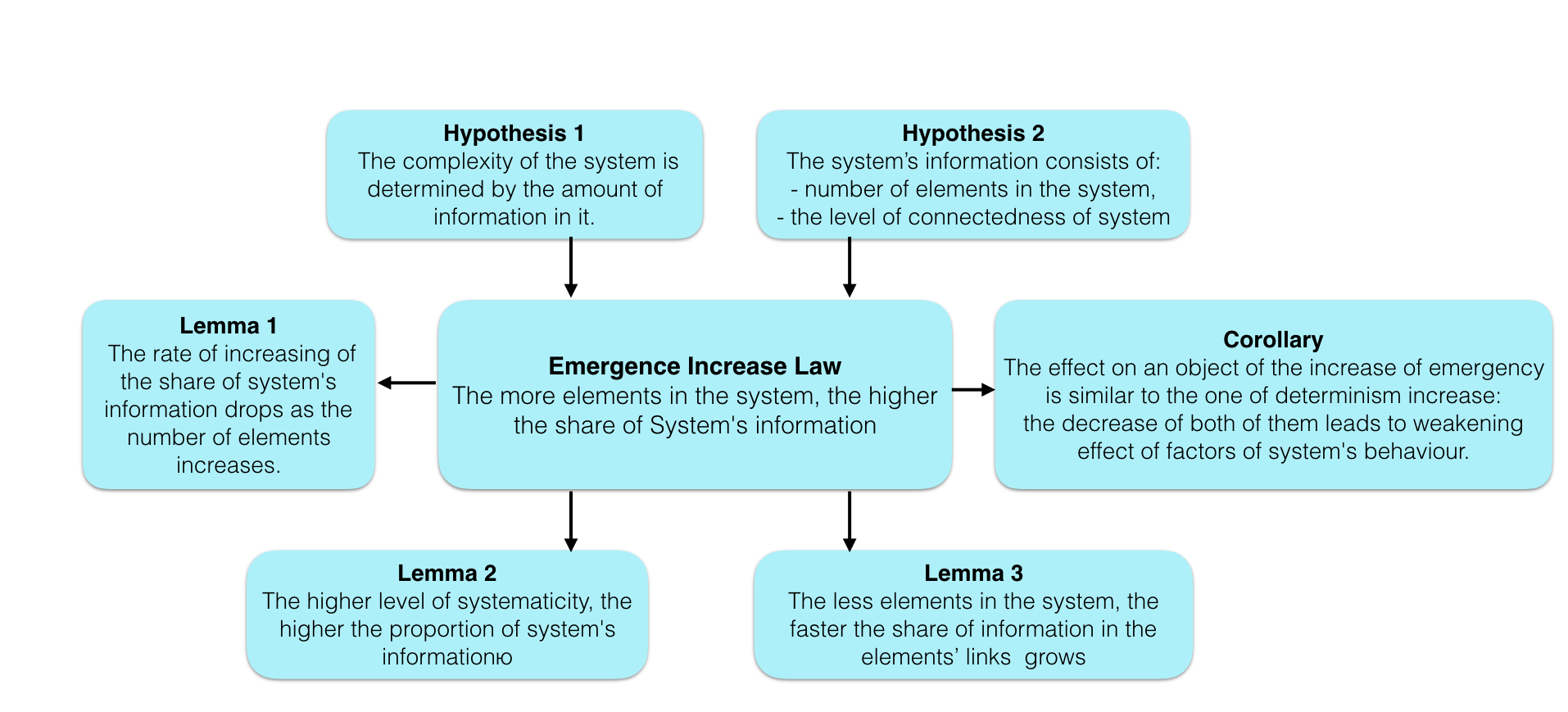
in other words, it consists of classical and synergic parts. The system’s information that we obtain from an object via STI approach is actually information on all possible configurations of the system. Prof. Lucenko [Lucenko, 2002] discovered a tendency for share of synergic information to raise as the number of elements increases and he propose to name it as the Law of emergence increase, illustrated at Figure 1.

Figure 1: Emergence Increase Law

Figure 2: Illustration of the concept of the Information Neural Bayesian approach based on the STI

The classical Harkevich formula is

$$I_{ij}=\log\frac{P_{ij}}{P_{j}},$$ (4)

where $P_{ij}$ is the probability of attaining target $J$ after getting message about feature $i$ and $P_{j}$ is the probability of attaining target (class) $j$ without any information. This concept does not take into account the cardinality of space of future configurations of the object, while they can be taken into consideration by involving the classical and synergic Hartley’s formulas, nevertheless it does not allow to obtain the quantity of information in bits. To solve that problem, we take for each feature $i,\ 1\leq i\leq M$ and class $j,\ 1\leq j\leq W$ approximate the probabilities $P_{ij}$ and $P_{j}$ through frequencies:

$$P_{ij}=\frac{N_{ij}}{N_{i}},\ \ P_{i}=\frac{N_{i}}{N},\ \ P_{j}=\frac{N_{j}}{N},$$ (5)

$$N_{i}=\sum^{W}_{i=1}N_{ij};\ \ N_{j}=\sum^{M}_{j=1}N_{ij};\ \ N=\sum^{W}_{i=1}\sum^{M}_{j=1}N_{ij}$$ (6)

where $N_{ij}$ is the total number of events like “condition $j$ was obtained after feature $i$ acting”, $N_{j}$ - total number of features, with which the condition $j$ was obtained, $N$ - total number of of various features for all final conditions. After placing into $I_{ij}=\log\frac{P_{ij}}{P_{j}}$ values $P_{ij}$ and $P_{j}$ we get the expression of value of information measured as its quantity:

$$I_{ij}(W,M)=\log_{2}\frac{N_{ij}N}{N_{i}N_{j}}$$ (7)

As it is known, the classical Shennon formula for quantity of information for events with varied probabilities transforms into Hartley’s formula with the condition that all events have the same probability, i.e. satisfy the basic property of conformance. So the same can be applied to the Harkevich formula, which means that in marginal case it should become Hartley’s formula (marginal case means that there is unique feature for every class (object’s condition) and vice versa, and all thesade classes have the same probability. In that case the quantity of information in each feature about belonging to classes is maximal and is equal to information calculated through Hartley’s formula. So, in case of one-to-one correspondence of features and classes:

General formula of Lutsenko formula and his emergence coefficient $\psi$ are:

$$I_{ij}=\log_{2}N^{\psi}=\log_{2}W^{\varphi},$$ (8)

$$\psi=\frac{\log_{2}W^{\varphi}}{\log_{2}N}$$ (9)

Taking it into account, authors suggest to add an emergence coefficient into the modified Harkevich formula. The resulting expression is named Lutsenko emergence information quantity formula:

$$I_{ij}(W,M,Z)=\log_{2}\Big{(}\frac{N_{ij}N}{N_{i}N_{j}}\Big{)}^{\psi},$$ (10)

where $\psi$ is Harkevich’s emergence coefficient, which defines the degree of determination of the object with the system’s organisation level $\varphi$, having $W$ pure conditions and $M$ features, on which the final condition is dependent, and Z is the maximal complexity calculated for each factor separately. $N$ observations on system’s behaviour were made. That generalisation can be performed in the following way:

$$I_{ij}=\log_{2}\Big{(}\frac{N_{ij}N}{N_{i}N_{j}}\Big{)}^{\psi}=\log_{2}\Big{(}\frac{N_{ij}N}{N_{i}N_{j}}\Big{)}^{\frac{\log_{2}W^{\varphi}}{\log_{2}N}}=$$ (11)

$$=\frac{\log_{2}W^{\varphi}}{\log_{2}N}\Big{(}\log_{2}\Big{(}\frac{N_{ij}}{N_{i}N_{j}}\Big{)}+\log_{2}N\Big{)}=$$ (12)

$$=\log_{2}\Big{(}\frac{N_{ij}}{N_{i}N_{j}}\Big{)}^{\frac{\log_{2}W^{\varphi}}{\log_{2}N}}+\log_{2}W^{\varphi}$$ (13)

The same calculations for the continuous case:

$$I=\log_{2}\int^{Z}_{z=q}\Big{(}\frac{G(W)}{G(z)\cdot G(W-z)}\Big{)}=$$

$$=\log_{2}\left\{G(W)\cdot\int^{Z}_{z=1}\frac{\,dz}{G(z)\cdot G(W-z)}\right\}=$$ (14)

$$=\log_{2}G(W)+\log_{2}\int^{Z}_{z=1}\frac{\,dz}{G(z)\cdot G(W-z)}$$

And finally:

$$I=\log_{2}G(W)+\log_{2}\int^{Z}_{z=1}\frac{\,dz}{G(z)\cdot G(W-z)}=I(W)+I(W,Z)$$ (15)

Generalised Kharkevich [1] formula also satisfies correspondence principle, i.e, transforms into Hartley’s formula: $\log\frac{P_{ij}}{P_{j}}=\log\frac{N_{ij}N}{N_{i}N_{j}}=\log N.$ In the marginal case, when every class (condition of the object) corresponds only one feature, and for every feature - one class, $\forall\ \ N_{i}j=N_{i}=N_{i}=1$ these classes and features have the same probabilities.

4.3 System Emergence Coefficient

General formula of Lutsenko for Harkevich emergence coefficient:

$$\psi=\frac{\log_{2}W^{\varphi}}{\log_{2}N}$$ (16)

where $\varphi=\frac{\log_{2}\sum^{Z}_{m=1}C^{m}_{W}}{\log_{2}W}$.

$\psi$ varies from 0 to 1 and determines the degree of determination of the system:

1. $\psi=1$ corresponds to absolutely determined system, behaviour of which depends on the minimal number of features.

2. $\psi=0$ corresponds to totally random system.

3. $0<\psi<1$ corresponds to system, where there are more features than classes and none of them plays the key role in determining the class.

Professor Lutsenko[4] proposed coefficients representing the degree of determination of the possible state of the object with a set of features at the system organization level $\varphi$. Nevertheless, as it seems hard to evaluate, it was decided to omit that concept and admit the coefficient $\varphi$ to be equal 1 (minimum level of complexity).

$$\psi=\frac{\log_{2}W}{\log_{2}N}$$ (17)

Straightforward way to calculate it is to consider all possible of combinations and classes, and for each one to evaluate the amount of information. Evidently, it will require enormous calculations.

$$\psi=\frac{\log_{2}W^{\varphi}}{\log_{2}N}=\frac{\log_{2}W^{\frac{log_{2}\sum_{m=1}^{Z}C^{W}_{m}}{\log_{2}W}}}{\log_{2}N}$$ (18)

The Lucenko-Artemov formula for emergence coefficient of system:

$$\psi=\frac{log_{2}\sum^{Z}_{m=1}C_{W}^{m}}{\log_{2}N}$$ (19)

The value obtained is the emergence coefficient of the system for the real level of complexity. The optimal solution is to consider only relevant combinations of feature-classes, dividing them into groups by complexity, up to which the combinations will be evaluated. There are two approaches for calculation the complexity Z. The first one for each feature takes the number of classes the feature corresponds to (gives positive amount of information). The number of classes represents the complexity, up to which the combinations of classes will be calculated. The second method is to divide all features and classes into groups with the same number of features as well as classes. The idea is to take all classes to whom the feature corresponds and select other features which correspond to the same classes. The key point is that it helps to build one-to-one correspondence between features and classes within that group. Finally we obtain limited number of features $i$ or groups of features $i\in g(\sum_{g}i=|M|$, where $M$ is the number of features), which are acting collectively $N_{g}$ times in the same number of classes $W_{g}$. That means for given features maximal complexity is $Z_{g}=W_{g}$. So $\sum^{Z_{g}}_{m=1}W_{g}=2^{Z_{g}}-1|Z_{g}=W_{g},g\in M$, and we get the final expression for the coefficient of emergence for each group:

$$\psi_{g}=\frac{log_{2}(2^{W_{g}}-1)}{\log_{2}N_{g}}$$ (20)

The coefficient is normalised by the following rule:

$$\psi_{g}\ =\ \begin{cases}1,&\text{if}\ W_{g}\textgreater\log_{2}2N\\ \frac{log_{2}(2^{W_{g}}-1)}{\log_{2}N},&\text{otherwise}\end{cases}$$ (21)

Formula 21 is the Artemov-Lucenko emergence coefficient, for the system of features, aggregated by the maximal level of of system’s complexity.

4.4 Application to neural networks

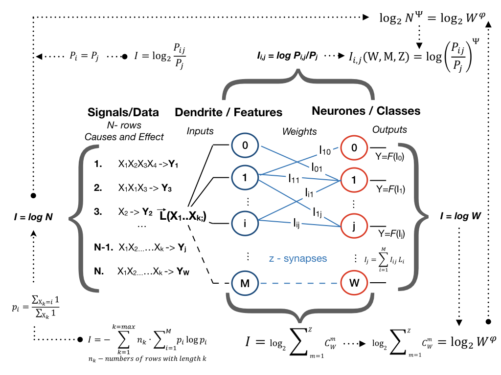
The essence of the proposed approach shows its best application to neural networks. The main idea is that the quantity of information, calculated for all feature-class pairs can be expressed in network’s weights, so they gain a meaning instead of being simply empirical parametrs. It explains the given name ”Informational Neurobayesian” for the approach. Every weight represents quantity of information - the object with the feature $i$ activates given neuron $j$:

$$I_{ij}=\psi_{i}\ \log{\frac{P_{ij}}{P_{j}}},$$ (22)

where $\psi_{i}$ - coefficient of emergence of the system for feature $i$.

Figure 3: Summation Process Architecture

In the scheme above the $L_{i}$ is $i$-th object’s feature. $\vv{L}\{X_{1},...,X_{k}\}$– a vector of object features:

$$L_{i}\ =\ \begin{cases}1,&\text{if}\ X_{k}\geq\epsilon\\ 0,&\text{otherwise}\end{cases}$$ (23)

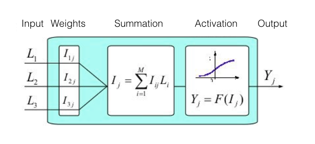
For every object with a given set of features the neural network chooses over all classes the one with maximal value of the activation function, represented as an activated sum by all features. The process is illustrated in Figure 3.

$$S_{j}=\sum^{M}_{j=1}I_{ij}\cdot L_{i}+\text{bias},\ \text{bias}=I_{0}$$ (24)

Bias is a parameter for activation of class. It allows to solve two problems: 1. To set a minimum threshold of neuron activation. 2. Allows integration with other models.

$$j^{*}=\arg\max_{j}f(S_{j})$$ (25)

$$y=f(S_{j*})$$ (26)

The Y is a chosen class for the given features, $f$ is activation function. The whole workflow is presented in Figure 2.

4.4.1 Generalised EM-Algorithm for INA

EM-algorithm consists of two steps iteration repetions. On the E-step expected hidden variables values are calculated using current estimate of parameters. On the M-step likeli- hood is maximised and new parameters vectors estimate is being obtained based on their current values and hidden variables vector.

Step 0: Calculate a frequency matrix for input data.

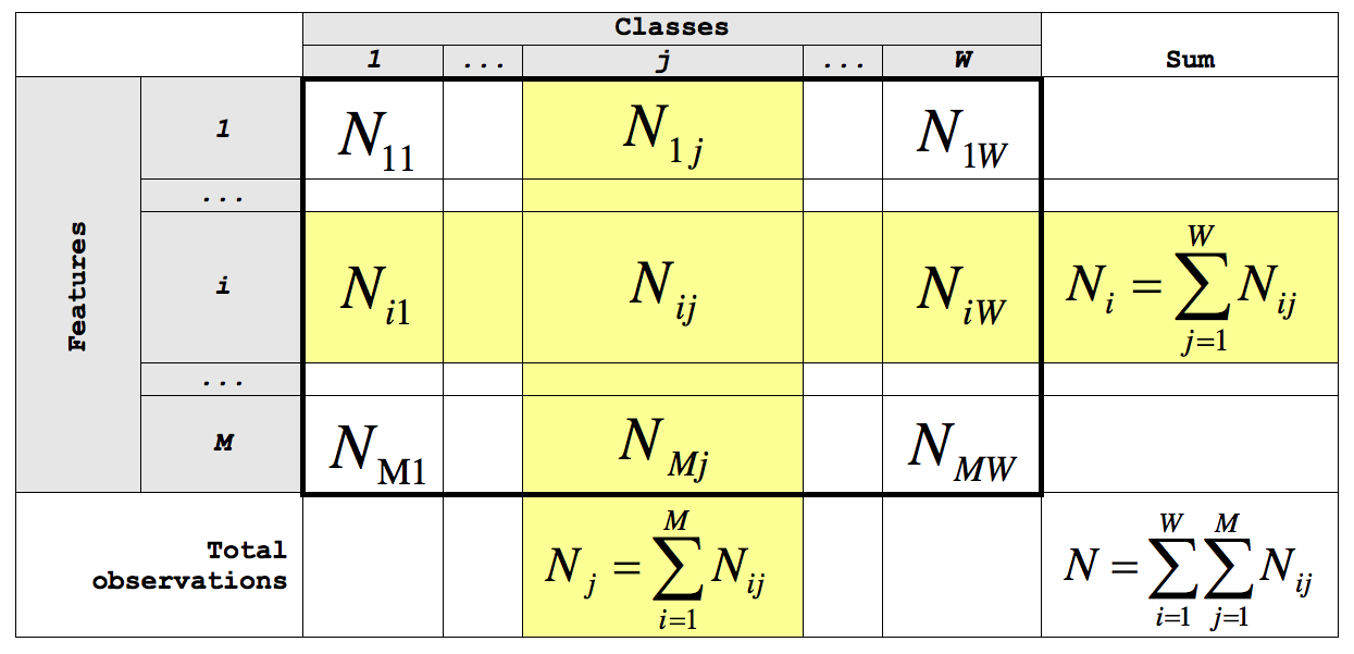
Unique features $M$ and classes $W$ are determined in training data and their frequency table which reflects the distribution of parameters $N_{ij}$ - number of features $i\in M$ for each class $j\in W$. Also $Z_{g}$ parameter (number of classes, in which a features group $g$ is active) is determined during this step.

Figure 4: Frequency matrix

Step E: Creating informational neurobayesian model.
During the E-step expected value of hidden variables $x_{i}$ by current estimation of parameter vector $N_{ij}$ is evaluated. The data is represented in Figure 4. and the output is organised in the same way, as presented in Figure 5.

$$I_{i,j}(W,M,Z)=\log\big{(}\frac{N_{i,j}N}{N_{i}N_{j}}\big{)}^{\psi_{g}}$$ (27)

$$\psi_{g}=\frac{log_{2}(2^{W_{g}}-1)}{\log N_{g}}$$ (28)

$$I_{i,j}(W,M,Z)\rightarrow\max_{Z}$$ (29)

Figure 5: Informational neurobayesian model

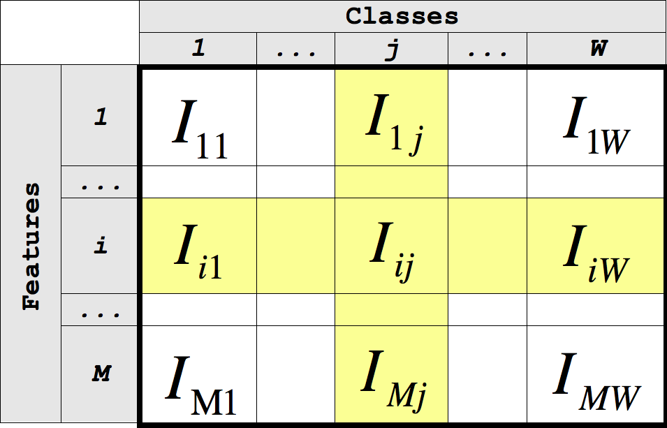
Step M: Model maximisation by Van Rijsbergen’s effectiveness measure (F-measure).

1. Calculate $E(F_{micro}):$

   Calculate average micro $F$-measure for each observed class $j_{l}\in W$ based on training set, comparing the result with $j_{t}$ - test dataset for object’s features vector with the same set of features, $t$ stands for test data, $l$ - data the model has been trained on («model has learnt»).

   $$E(F_{\text{micro}})=\frac{\sum_{k}F_{j_{t}}}{k}$$ (30)

   $$F_{j_{t}}=(1+\beta)^{2}\frac{\text{ precision}_{j_{t}}\times\text{ recall}_{j_{t}}}{\beta^{2}\text{ precision}_{j_{t}}+\text{ recall}_{j_{t}}}$$ (31)

   $$0<\beta<1,$$

   $$j_{t}=\arg\max F(S_{j_{t}})$$ (32)

2. For each $j_{t}\in W,$ where $F_{j_{t}}<\ E(F_{j_{t}})$, i.e. $j_{l}\neq\arg\max F(S_{j_{t}})$ or $S_{j_{t}}<S_{j_{l}}.$
   2.1 Determine $j^{*}_{t}$ and $j^{*}_{l}$ - correct class for the set of features $L_{i}$, $i\in M$.
   2.2 Exclude all objects $L_{i}$ with the same set of features, but $j^{*}_{t}\neq j^{*}_{l}$ classes
   2.3 For remaining objects $L_{i}$ change quantity of information for each feature, acting in given class $I_{j_{l}}\rightarrow I_{j^{*}_{l}}$, so that $S_{j_{l}}\rightarrow\max S_{j^{*}_{l}}$

   $$j_{l}=\arg\max F(S_{j^{*}_{l}})$$

   
   

   2.4 Calculate

   $$E(F^{*}_{\text{micro}})=\frac{\sum_{k}F_{j_{t*}}}{k}$$ (33)

   The updated model is checked for improvement on wrongly classified objects.
   2.5 Continue until $E(F^{*}_{\text{micro}})\ \textgreater\ E(F_{\text{micro}})$

Table 1: Experiments Results

Model	MNIST	House Prices	Emotions in text	Russian words	Russian words
Problem	Hand-written	Real Estate	Determining emotions	Word recognition by letters and bigramms.
	digits recognition	Valuation	(by Ecman), in text.
Features	2 815	809	19 121	1042	1042
Classes	11	658	8	5 099 300	5 099 300
Parameters (weights)	30 965	532 322	152 968	6 313 470 600	6 313 470 600
Model Size (Mb)	-	1,89		634,94	634,94
Training data size (Mb)	74,9	0,53	2,85	505,43	505,43
Training data, rows	42 000	1460	8 682	5 099 300	5 099 301
Learning Type	E (1 epoch)	E (1 epoch)	E (1 epoch)	E (1 epoch)	EM
Brain2 v.	1.0	2.0	2.0	3.0	3.0
Result	CA =0,81	RMSE=0,42	F1 = 0,81	F1=0,97	F1=0.98
Time	20 min	2 min 33 sec	6 min 4 sec	2 h, 35 min	2 h, 49 min

Table 2: Weights calculating methods comparison

	Gradient Descent applied to neural networks	Neurobayesian Approach	Informational Neurobayesian Approach
Optimisation framework	Backpropagation	Stochastic Gradient Descent with reparameterization trick.	EM - algorithm applied to quantity of emergent information
Weights Interpretation	Weights are just numbers	Weights represent probabilities	Weights represent quantity of information
Complexity	$O(n^{2})$	$O(n)$	$O(\log n)$ - E-step $O(n\log n)$ - M-step
Advantages	Wide range for applications	Decreased computation complexity	1.The E-step gives satisfactory results. (no need to do M-step) 2. Arithmetical operations can be applied to weights as they represent the quantity of information. 3.Applicable for training complex models just on CPU.

5 Experiments

For conducting the tests we used Brain2 - a software platform implementing Informational Neurobayesian Approach. The biggest built neuromodel is aimed at word recognition by letter and bigrams in Russian language for 100 000 words – it consists of 1042 features and 5 099 300 classes, which makes the total number of parameters 6.3 bln (weight coefficients). An important factor here is that it took only 2 h 35 min to build the model on an average server without GPU (205 GFlops, 8 cores CPU). In comparison, the Google Brain biggest neural network consists of 137 billion parameters, but if we consider the needed resources – only for 4.3 bln parameters it took them 47 hours with 16-32 Tesla K40 GPUs (1220 GFlops) [8][Shazeer N, 2017]. On other basic machine learning tasks such as MNIST and House Prices our models have shown an acceptable result – 0.81 on MNIST (Kaggle task) with the best 1.0; and 0.42 on House Prices with the best one at 0.06628 (For one epoch). It is important to note that we did not set the task to achieve the best possible result and have trained the model as is. Instead, we have concentrated on a more difficult problem, connected with natural text – reconstruction of words with errors and finding answers on questions, where we have reached accuracy close to 1. Experiment results are presented in Table 1.

6 Conclusion

In the paper the INA method aimed to cope with complex classification problems more intelligently than currently used analytical and numerical methods was described. Its ability to be applied to neural networks and provided experiments showed opportunities for the suggested method to simplify training process in various classification problems and achieve at least the same performance with less computational costs. The results of the experiments are presented in Table 1. And the summary of comparison with other method is presented in Table 2.

The additive properties of the amount of information allow not only to explain the correctness of addition of weights while choosing a class within a single model (layer), but also to link different models (layers), transferring values ​​of the amount of information from one input to another. In addition, every information neuromodel can be trained independently. Eventually it makes possible to facilitate the construction of super-neural networks - multilevel (and multi-layer) neural networks, where each input of the neuron is a neural network of a lower order (from the position of information amount). The proposed information approach makes it possible to obtain an acceptable level of quality of the model (F1 $>$ 0.6, for 1 epoch), even on relatively small data. And given the low complexity $(O(n))$ of the learning algorithm , the INA opens new horizons to the training of superneuromodels on conventional (not super) computers.

In our opinion, the INA combines in itself a general philosophical view presented by such cognitive scientists as D. Chalmers[6] (as each layer represents a level of cognition, influencing a higher cognition level), V. Nalimov (in the works on the [9]probabilistic model of language [Nalimov, 1990]) and the pragmatic concept of meaning - the amount of information in the cause for a given consequence required for making a managerial decision [5] (Ashby[7] , Wiener, U. Hubbard).

References

- [1] Harkevich A. On information value. Cybernetics problems.№ 4, 2009.
- [2] Vetrov D. Bayesian Methods in Machine Learning. http://bit.ly/2eE0Tfj,http://bayesgroup.ru/, 2016.
- [3] Lutsenko E.V. Conceptual principles of the system (emergent) information theory and its application for the cognitive modelling of the active objects (entities). IEEE International Conference on Artificial Intelligence System, 2002.
- [4] Lutsenko E.V. System information theory and nonlocal interpratable feedforward neural net. Polytechnical network electronic scientific journal of the Kuban State Agrarian University, 2003.
- [5] Uladzimir Kharkevich Fausto Giunchiglia and Ilya Zaihrayeu. Concept Search. Oxford University Press.
- [6] Chalmers D. J. The conscious mind: In search of a fundamental theory. Oxford University Press, 1996.
- [7] Ashby W. R. An introduction to cybernetics. Chapman and Hall Ltd, 1961.
- [8] Mirhoseini A. Maziarz K. Davis A. Le Q. Hinton G. Shazeer, N. and J. Dean. Outrageously large neural networks: The sparsely-gated mixture-of-experts layer. arXiv preprint, 2017.
- [9] Nalimov V. V. Spontaneity of Consciousness: Probabalistic Theory of Meanings and Semantic Architectonics of Personality. 1990.