SERENADE: A Parallel Randomized Algorithm for Crossbar Scheduling in Input-Queued Switches

Abstract

Most of today’s high-speed switches and routers adopt an input-queued crossbar switch architecture. Such a switch needs to compute a matching (crossbar schedule) between the input ports and output ports during each switching cycle (time slot). A key research challenge in designing large (in number of input/output ports $N$) input-queued crossbar switches is to develop crossbar scheduling algorithms that can compute “high quality” matchings – i.e., those that result in high switch throughput (ideally $100\%$) and low queueing delays for packets – at line rates. SERENA is one such algorithm: it outputs excellent matching decisions that result in $100\%$ switch throughput and reasonably good queueing delays. However, since SERENA is a centralized algorithm with $O(N)$ computational complexity, it cannot support switches that both are large and have a very high line rate per port. In this work, we propose SERENADE (SERENA, the Distributed Edition), a parallel iterative algorithm that emulates SERENA in only $O(\log N)$ iterations between input ports and output ports, and hence has a time complexity of only $O(\log N)$ per port. We prove that SERENADE can exactly emulate SERENA. We also propose an early-stop version of SERENADE, called O-SERENADE, to only approximately emulate SERENA. Through extensive simulations, we show that O-SERENADE can achieve 100% throughput and that it has similar as or slightly better delay performance than SERENA under various load conditions and traffic patterns.

1 Introduction

The volumes of network traffic across the Internet and in data-centers continue to grow relentlessly, thanks to existing and emerging data-intensive applications, such as Big Data analytics, cloud computing, and video streaming. At the same time, the number of network-connected devices also grows explosively, fueled by the wide adoption of smart phones and the emergence of the Internet of things. To transport and “direct” this massive amount of traffic to their respective destinations, switches and routers capable of connecting a large number of ports (called high-radix), and operating at very high per-port speeds are badly needed. Motivated by this rapidly growing need, much research has been devoted to, and significant breakthroughs made, on the hardware designs for fast high-radix switching fabrics recently (e.g., [1, 2]). Indeed, these recent breakthroughs have made fast high-radix switching hardware not only technologically feasible but also economically and environmentally (more energy-efficient) favorable, as compared to low-radix switching hardware [1].

Most of today’s switches and routers adopt an input-queued crossbar switch architecture. fig: input-queued-switch shows a generic input-queued switch employing a crossbar to interconnect $N$ input ports with $N$ output ports. Each input port has $N$ Virtual Output Queues (VOQs). A VOQ $j$ at input port $i$ serves as a buffer for the packets going into input port $i$ destined for output port $j$. The use of VOQs solves the Head-of-Line (HOL) blocking issue [3], which severely limits the throughput of the switching system.

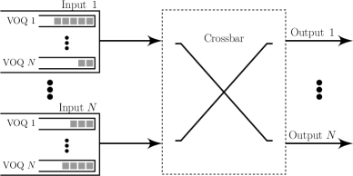
Figure 1: An input-queued crossbar switch.

1.1 Matching Problem and SERENA Algorithm

In an input-queued crossbar switch, each input port can be connected to only one output port, and vice versa, in each switching cycle, or time slot. Hence, it needs to compute, per time slot, a one-to-one matching between input and output ports. One major research challenge in designing high-radix input-queued crossbar switches is to develop algorithms that can compute “high quality” matchings – i.e., those that result in high switch throughput (ideally $100\%$) and low queueing delays for packets – at line rates.

Unfortunately, there appears to be a tradeoff between the quality of a matching and the amount of time needed to compute it (i.e., time complexity). For example, when used for crossbar scheduling, Maximum Weight Matching (MWM), with a suitable weight measure, is known to result in 100% switch throughput [4] and is conjectured to have the optimal delay performance [5]. Each matching decision however takes $O(N^{3})$ time to compute [6].

Ideally, a crossbar scheduling algorithm should have time complexity much lower than $O(N^{3})$, but performance close to that of MWM. SERENA [7, 8] is one such algorithm. SERENA produces excellent matching decisions that result in $100\%$ switch throughput and reasonably good queueing delay. However, it is a centralized algorithm with $O(N)$ time complexity. When $N$ is large, this complexity is too high to support very high link rates. Hence, as stated in [7, 8], SERENA is designed for high-aggregate-rate switches – i.e., those that have either a large number of ports or a very high line rate per port – but not for those that have both. While parallelizing the SERENA algorithm seems to be an obvious solution to this scalability problem, we will show in subsec: merge that a key procedure in SERENA, namely MERGE, is monolithic in nature, making SERENA hard to parallelize.

1.2 Parallelizing SERENA via SERENADE

In this work, we propose SERENADE (SERENA, the Distributed Edition), a parallel iterative algorithm that emulates each matching computation of SERENA using only $O(\log N)$ iterations between input ports and output ports. Hence, each input or output port needs to do only $O(\log N)$ work to compute a matching, making SERENADE scalable in both the switch size and the line rate per port.

SERENADE consists of two stages: knowledge-discovery stage and distributed binary search stage. The knowledge-discovery stage uses a knowledge-discovery procedure, which has at most $1\!+\!\log_{2}N$ iterations, to gather information at each input port. After this stage, some input ports might be able to make the same decisions as they would under SERENA, whereas other input ports are not able to do so. Then, in the distributed binary search stage, those input ports will also be able to make the same matching decisions as they would do under SERENA by performing an additional distributed binary search, which has at most $\log_{2}N$ iterations, guided by the information gathered during the knowledge-discovery stage. We prove that SERENADE exactly emulates SERENA.

SERENADE overcomes the aforementioned challenge of parallelizing SERENA, namely the monolithic nature of the MERGE procedure, by making do with less. More specifically, we will show toward the end of subsubsec:knowledge-sets, in SERENADE, after its $O(\log N)$ iterations, each input port has much less information to work with than the (central) switch controller in SERENA. In other words, SERENADE does not precisely parallelize SERENA, in that it does not duplicate the full information gathering capability of SERENA; rather, it gathers just enough information needed to make a matching decision that is either exactly or almost as wise. This making do with less is a major innovation and contribution of this work.

To reduce the complexities, we propose an early-stop version of SERENADE, called O-SERENADE, to approximately emulate SERENA. O-SERENADE gets rid of the distributed binary search and only approximately emulates SERENA by making opportunistic matching decisions after the knowledge-discovery stage. Despite this approximation, the delay performance of O-SERENADE is similar to or slightly better than that of SERENA, under various load conditions and traffic patterns.

The rest of the paper is organized as follows. In sec: background, we offer some background on input-queued crossbar switches. In sec: serena-and-merge, we describe in detail the MERGE procedure in SERENA that is to be parallelized in SERENADE. In sec: serenade, we provide an overview of SERENADE, before zooming in on the knowledge-discovery stage in sec:knowledge-discovery, its augmentation, i.e., the leader election in sec:leader-election, and the distributed binary search stage in sec:bs. In subsec: o-serenade, we introduce the early-stop version, O-SERENADE. In sec:evaluation, we evaluate the performance of SERENADE. In sec: related-work, we provide a brief survey of related work before concluding the paper in sec: conclusion.

2 System Model and Background

We assume that all incoming variable-size packets are segmented into fixed-size packets, which are then reassembled when leaving the switch. Hence we consider the switching of only fixed-size packets in the sequel, and each such fixed-size packet takes exactly one time slot to transmit. We also assume that both the output ports and the crossbar operate at the same speed as the input ports. Both assumptions above are widely adopted in the literature [9, 4, 10, 8, 11]. Like in [8], we further assume that the arrival processes for those fixed-size packets are i.i.d. Bernoulli.

An $N\!\times\!N$ input-queued crossbar switch is usually modeled as a weighted complete bipartite graph $G(I\bigcup O)$, with the $N$ input ports and the $N$ output ports represented as the two disjoint vertex sets $I\!=\!\{I_{1},I_{2},\dots,I_{N}\}$ and $O\!=\!\{O_{1},O_{2},\dots,O_{N}\}$ respectively. Each edge $(I_{i},O_{j})$ corresponds to the $j^{th}$ VOQ at input port $i$ and its weight is defined as the number of packets in the VOQ. We denote this edge also as $I_{i}\!\rightarrow\!O_{j}$ when its direction is emphasized.

A valid schedule, or matching, is a set of edges between $I$ and $O$ in which no two distinct edges share a vertex. The weight of a matching is defined as the total weight of all edges belonging to the matching. We say that a matching is full if all vertices in $G(I\bigcup O)$ are an endpoint of an edge in the matching, and is partial otherwise. Clearly, in an $N\!\times\!N$ switch, any full matching contains exactly $N$ edges.

3 SERENA

To explain SERENADE, we first explain SERENA, the algorithm it parallelizes. SERENA consists of two steps. The first step is to derive a full matching $R(t)$ from the set of packet arrivals $A(t)$. The second step is to merge $R(t)$ with the full matching $S(t-1)$ used in the previous time slot, to arrive at the full matching $S(t)$ to be used for the current time slot $t$. After we briefly describe the first step, we will focus on the second step, MERGE, in the rest of this section.

In [8], the set of packet arrivals $A(t)$ is modeled as an arrival graph, which we denote also as $A(t)$, as follows: an edge $(I_{i},O_{j})$ belongs to $A(t)$ if and only if there is a packet arrival to the corresponding VOQ at time slot $t$. Note that $A(t)$ is not necessarily a matching, because more than one input ports could have a packet arrival (i.e., edge) destined for the same output port at time slot $t$. Hence in this case, each output port prunes all such edges incident upon it except the one with the heaviest weight (with ties broken randomly). The pruned graph, denoted as $A^{\prime}(t)$, is now a matching.

This matching $A^{\prime}(t)$, which is typically partial, is then randomly populated into a full matching $R(t)$ by pairing the yet unmatched input ports with the yet unmatched output ports in a round-robin manner. Although this POPULATE procedure alone, with the round-robin pairing, has $O(N)$ computational complexity, we will show in subsec: parallel-population that it can be reduced to the computation of prefix sums and solved using the classical parallel algorithm [12] whose time complexity in this context is $O(\log N)$ per port.

3.1 Overview of The MERGE Procedure

In this section, we explain the MERGE procedure through which SERENA selects heavier edges for $S(t)$ from both $R(t)$ with $S(t-1)$, so that the weight of $S(t)$ is larger than or equal to those of both $R(t)$ and $S(t-1)$. We color-code and orient edges of $R(t)$ and $S(t-1)$, like in [8], as follows. We color all edges in $R(t)$ red and all edges in $S(t-1)$ green, and hence in the sequel, rename $R(t)$ to $S_{r}$ (“r” for red) and $S(t-1)$ to $S_{g}$ (“g” for green) to emphasize the coloring. We drop the henceforth unnecessary term $t$ here with the implicit understanding that the focus is on the MERGE procedure at time slot $t$. We also orient all edges in $S_{r}$ as pointing from input ports (i.e., $I$) to output port (i.e., $O$) and all edges in $S_{g}$ as pointing from output ports to input ports. We use notations $S_{r}(I\!\rightarrow\!O)$ and $S_{g}(O\!\rightarrow\!I)$ to emphasize this orientation when necessary in the sequel. Finally, we drop the term $t$ from $S(t)$ and denote the final outcome of the MERGE procedure as $S$.

Now we describe how the two color-coded oriented full matchings $S_{r}(I\!\rightarrow\!O)$ and $S_{g}(O\!\rightarrow\!I)$ are merged to produce the final full matching $S$. The MERGE procedure consists of two steps. The first step is to simply union the two full matchings, viewed as two subgraphs of the complete bipartite graph $G(I\bigcup O)$, into one that we call the union graph and denote as $S_{r}(I\!\rightarrow\!O)\bigcup S_{g}(O\!\rightarrow\!I)$ (or $S_{r}\bigcup S_{g}$ in short). In other words, the union graph $S_{r}(I\!\rightarrow\!O)\bigcup S_{g}(O\!\rightarrow\!I)$ contains the directed edges in both $S_{r}(I\!\rightarrow\!O)$ and $S_{g}(O\!\rightarrow\!I)$.

It is a mathematical fact that any such union graph can be decomposed into disjoint directed cycles [8]. Furthermore, each directed cycle, starting from an input port $I_{i}$ and going back to itself, is an alternating path between a red edge in $S_{r}$ and a green edge in $S_{g}$, and hence contains equal numbers of red edges and green edges. In other words, this cycle consists of a red sub-matching of $S_{r}$ and a green sub-matching of $S_{g}$. Then in the second step, for each directed cycle, the MERGE procedure compares the weight of the red sub-matching (i.e., the total weight of the red edges in the cycle), with that of the green sub-matching, and includes the heavier sub-matching in the final merged matching $S$.

Illustrative Example. To illustrate the MERGE procedure by an example, fig: cycles-in-union shows the union graph of the following two full matchings over a $16\times 16$ bipartite graph (crossbar). The number around each edge is its weight. The first full matching $S_{r}(I\!\rightarrow\!O)$, written as a permutation with input port numbers ($1$ as $I_{1}$, $2$ as $I_{2}$, and so on) at the top and output port numbers at the bottom ($1$ as $O_{1}$, $2$ as $O_{2}$, and so on), is $\setcounter{MaxMatrixCols}{16}\begin{pmatrix}1&2&3&4&5&6&7&8&9&10&11&12&13&14&15&16\\ 6&5&1&14&15&7&16&12&10&3&9&4&2&11&13&8\end{pmatrix}$. We denote this permutation as $\sigma_{r}$. For example, $\sigma_{r}$ mapping (input port) $3$ to (output port ) $1$ corresponds to the red edge $I_{3}\!\rightarrow\!O_{1}$ in fig: cycles-in-union (i.e., $I_{3}$ pairing with $O_{1}$ in $S_{r}$, the “red” matching). The second full matching $S_{g}(O\!\rightarrow\!I)$, written as a permutation with output port numbers at the top and input port numbers at the bottom, is $\setcounter{MaxMatrixCols}{16}\begin{pmatrix}1&2&3&4&5&6&7&8&9&10&11&12&13&14&15&16\\ 4&9&12&3&8&1&15&10&2&6&7&5&13&14&16&11\end{pmatrix}$. We denote this permutation as $\sigma^{-1}_{g}$. The union graph contains three disjoint directed cycles that are of lengths $22,8,2$ respectively. Now, we illustrate the MERGE procedure on the leftmost cycle in fig: cycles-in-union. It is not hard to check that the total weight of the red sub-matching in this cycle is $82$ and that of the green sub-matching is $84$. Then, the heavier sub-matching, i.e., the green one, is included into the final merged matching $S$.

The standard centralized algorithm for implementing the MERGE procedure is to linearly traverse every cycle once, by following the directed edges in the cycle, to obtain the weights of the green and the red sub-matchings that comprise the cycle [8]. Clearly, this algorithm has a computational complexity of $O(N)$. The primary contribution of SERENADE is to reduce this complexity to $O(\log N)$ per input/output port through parallelization.

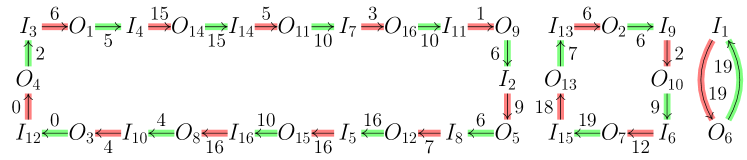
Figure 2: Cycles in $S_{r}(I\!\rightarrow\!O)\bigcup S_{g}(O\!\rightarrow\!I)$: Edges with red and green shadows are from $S_{r}(I\!\rightarrow\!O)$ and $S_{g}(O\!\rightarrow\!I)$ respectively.

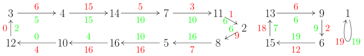
Figure 3: Combinatorial Cycles correspond to the cycles in fig: cycles-in-union.

3.2 A Combinatorial View of MERGE

In this section, to better describe MERGE under SERENADE however, we introduce a combinatorial view of MERGE, through which the MERGE procedure can be very succinctly characterized by a single permutation $\sigma\triangleq\sigma_{g}^{-1}\circ\sigma_{r}$, the composition of the two aforementioned full matchings $S_{r}(I\rightarrow O)$ and $S_{g}(O\rightarrow I)$ written as permutations. We do so using the example shown in  fig: cycles-in-union. It is not hard to verify that, in this example, $\sigma\triangleq\sigma_{g}^{-1}\circ\sigma_{r}\!=\!\setcounter{MaxMatrixCols}{16}\begin{pmatrix}1&2&3&4&5&6&7&8&9&10&11&12&13&14&15&16\\ 1&8&4&14&16&15&11&5&6&12&2&3&9&7&13&10\end{pmatrix}$. We then decompose this permutation $\sigma$ into disjoint combinatorial cycles. In this example, $\sigma\!=\!(3\,4\,14\,7\,11\,2\,8\,5\,16\,10\,12)(13\,9\,6\,15)(1)$, and its cycle decomposition graph, which contains precisely these three combinatorial cycles, is shown in fig: comb-cycles.

Note there is a one-to-one correspondence between the graph cycles (of the union graph $S_{r}\bigcup S_{g}$) shown in fig: cycles-in-union and the combinatorial cycles of $\sigma$ shown in fig: comb-cycles. For example, cycle $I_{3}\!\!\rightarrow\!\!O_{1}\!\!\rightarrow\!\!I_{4}\!\!\rightarrow\!\!O_{14}\!\!\rightarrow\!\!\cdots\!\!\rightarrow\!\!O_{3}\!\!\rightarrow\!\!I_{12}\!\!\rightarrow\!\!O_{4}\!\!\rightarrow\!\!I_{3}$, the leftmost cycle in fig: cycles-in-union, corresponds to the leftmost combinatorial cycle $(3\,4\,14\,7\,11\,2\,8\,5\,16\,10\,12)$ in fig: comb-cycles. Note that two consecutive edges – one belonging to the red matching $S_{r}$ and the other to the green matching $S_{g}$ – on the graph cycle “collapse” into an edge on the corresponding combinatorial cycle. For example, two directed edges $(I_{3},O_{1})$ ($\in S_{r}$) and $(O_{1},I_{4})$ ($\in S_{g}$) in fig: cycles-in-union collapsed into the directed edge from (input port) $3$ to (input port) $4$ in the combinatorial cycle $(3\,4\,14\,7\,11\,2\,8\,5\,16\,10\,12)$ in fig: comb-cycles. Hence each combinatorial cycle subsumes a red sub-matching and a green sub-matching that collapse into it. Note also that each vertex on the cycle decomposition graph corresponds to an input port. For example, vertex “3” in $(3\,4\,14\,7\,11\,2\,8\,5\,16\,10\,12)$ in fig: comb-cycles corresponds to input port $I_{3}$ in fig: cycles-in-union. Hence, we use the terms “vertex” and “input port” interchangeably in the sequel.

We assign a green weight $w_{g}(\cdot)$ and a red weight $w_{r}(\cdot)$ – to each combinatorial edge $e$ in the cycle decomposition graph – that are equal to the respective weights of the green and the red edges that collapse into $e$. For example, the green and red numbers around each edge shown in fig: comb-cycles represent its green and red weights respectively. We also define the green (or red) weight of a combinatorial cycle as the total green (or red) weight of all combinatorial edges on the cycle. Clearly, this green (or red) weight is equal to the weight of the green (or red) sub-matching this cycle subsumes. Under this combinatorial view, the MERGE procedure of SERENA can be stated as follows: For each combinatorial cycle of $\sigma$, we compare its red weight with its green weight, and include in $S$ the corresponding heavier sub-matching.

3.3 Walks on Cycles

Finally, we introduce the concept of walk on a cycle decomposition graph. It greatly simplifies the descriptions of SERENADE, as it will become clear later that SERENADE is all about how to emulate SERENA using information, each input port obtains, regrading a few walks with lengths of power of $2$. Recall that a walk in a general graph $G(V,E)$ is an ordered sequence of vertices, $v_{1}\!\!\rightarrow\!\!v_{2}\!\!\rightarrow\!\!\cdots\!\!\rightarrow\!\!v_{k}$ such that $(v_{j},v_{j+1})\!\in\!E$ for any $j\!\in\!\{1,2,\dots,k-1\}$; note that a walk, unlike a path, can traverse a vertex or edge more than once. Clearly, in the cycle decomposition graph of $\sigma$, every walk (say starting from a vertex $i$) circles around a combinatorial cycle (the one that $i$ lies on), and hence necessarily takes the following form: $i\!\!\rightarrow\!\!\sigma(i)\!\!\rightarrow\!\!\sigma^{2}(i)\!\!\rightarrow\!\!\cdots\!\!\rightarrow\!\!\sigma^{m}(i)$. For notational convenience, we denote this walk as $i\leadsto\sigma^{m}(i)$. For example, with respect to the combinatorial cycle $(3\,4\,14\,7\,11\,2\,8\,5\,16\,10\,12)$ in fig: comb-cycles, the walk $3\leadsto\sigma^{8}(3)$ represents $3\!\!\rightarrow\!\!4\!\!\rightarrow\!\!14\!\!\rightarrow\!\!7\!\!\rightarrow\!\!11\!\!\rightarrow\!\!2\!\!\rightarrow\!\!8\!\!\rightarrow\!\!5\!\!\rightarrow\!\!16$, which consists of $8$ directed edges on the cycle.

Generalizing this notation (of a walk), we define $\sigma^{m_{1}}(i)\!\leadsto\!\sigma^{m_{2}}(i)$ as the $(m_{2}\!-\!m_{1})$-edge-long walk $\sigma^{m_{1}}(i)\!\!\rightarrow\!\!\sigma^{(m_{1}\!+\!1)}(i)\!\!\rightarrow\!\!\cdots\!\!\rightarrow\!\!\sigma^{m_{2}}(i)$, where $m_{1}\!<\!m_{2}$ are integers, and both $m_{1}$ and $m_{2}$ could be negative. We define its red weight, denoted as $w_{r}(\sigma^{m_{1}}(i)\!\leadsto\!\sigma^{m_{2}}(i))$, as the sum of the red weights of all edges in $\sigma^{m_{1}}(i)\!\leadsto\!\sigma^{m_{2}}(i)$. Note that if an edge is traversed multiple times in a walk, the red weight of the edge is accounted for multiple times. The green weight of the walk, denoted as $w_{g}(\sigma^{m_{1}}(i)\!\leadsto\!\sigma^{m_{2}}(i))$, is similarly defined.

4 Overview of SERENADE

In this section, we provide a high-level overview of SERENADE. We first introduce the core idea of SERENADE that is based on an important concept called “discover”. Then, we give a high-level description of two algorithmic stages of SERENADE: knowledge-discovery stage and distributed binary search stage. For ease of presentation (e.g., no need to put floors or ceilings around each occurrence of $\log_{2}N$), we have assumed that $N$ is a power of $2$ throughout this paper; SERENADE works just as well when $N$ is not.

4.1 Core Idea of SERENADE

The core idea of SERENADE is for all vertices on a combinatorial cycle, or a designated vertex among them, to discover (defined next) itself or another vertex on the same cycle twice. As will be shown next in fact:disc, when this happens, these vertices will know precisely whether the green weight or the red weight of the cycle is larger, and hence will select the same heavier sub-matching as they would under SERENA. If this happens on every combinatorial cycle, then SERENADE exactly emulates SERENA.

Definition 1.

Given two vertices $i,j$ in any combinatorial cycle of $\sigma$, we say that vertex $i$ discovers vertex $j$ if $i$ learns the identity of $j$ and the weights of a walk from $i$ to $j$ or from $j$ to $i$.

By this definition, every vertex $i$ discovers itself, once at the beginning (i.e., before any algorithmic steps), via the empty (0-edge-long) walk from $i$ to $i$.

Lemma 1 (Property of “Discover”).

Let $i$ and $j$ be two vertices, which may or may not be the same vertex, on a combinatorial cycle of $\sigma$. If $i$ discovers $j$ twice via two different walks, then vertex $i$ knows precisely whether the green weight or the red weight of the cycle is larger.

Proof:

See app:proof-lemma-01. ∎

4.2 High-Level Description of SERENADE

As mentioned earlier, SERENADE consists of two algorithmic stages: knowledge-discovery stage and distributed binary search stage. In this section, we give the high-level descriptions of these two stages, deferring their details to subsec:knowledge-discovery and subsec:bs respectively.

Knowledge-Discovery Stage. The knowledge-discovery stage uses the standard technique of two-directional exploration with successively doubled distance in distributed computing [13]. The basic idea of the algorithm is for each vertex $i$ to exchange information, during the $k^{th}$ ($1\!\leq\!k\!\leq\!\log_{2}N$) iteration, with vertices “$(\pm 2^{k-1})$ $\sigma$-hops” away (i.e., $\sigma^{2^{k-1}}(i)$ and $\sigma^{-(2^{k-1})}(i)$) to discover two vertices “$(\pm 2^{k})$ $\sigma$-hops” away (i.e., $\sigma^{2^{k}}(i)$ and $\sigma^{-(2^{k})}(i)$). If either of the two vertices has been discovered twice by $i$, then, by fact:disc, we know that vertex $i$ can make the same matching decision as it would under SERENA. In the example shown in fig: comb-cycles, vertex $3$ communicates, during the $1^{st}$ iteration, with vertices $4\!=\!\sigma(3)$ and $12\!=\!\sigma^{-1}(3)$ to discover vertices $14\!=\!\sigma^{2}(3)$ and $10\!=\!\sigma^{-2}(3)$, and communicates, during the $2^{nd}$ iteration, with the newly-discovered vertices $14$ and $10$ to discover vertices $11=\sigma^{4}(3)$ and $5\!=\!\sigma^{-4}(3)$, and so on in the next $(\log_{2}N)\!-\!2$ iterations.

Distributed Binary Search Stage. After the $1\!+\!\log_{2}N$ iterations of the knowledge discovery, a vertex $i$, residing on a cycle, will discover a vertex on the same cycle twice and hence make the same matching decision as it would under SERENA, if the cycle is ouroboros (to be defined in subsec:ouroborous-cycle). However, not all cycles are ouroboros, as will be shown in subsec:ouroborous-cycle. Those and only those vertices, residing on non-ouroboros cycles, then perform an additional distributed binary search, the purpose of which is to let a designated vertex in each non-ouroboros cycle discover itself for a second time. We will show in sec:leader-election that the elections of those designated vertices (i.e., leader election) can be seamlessly embedded into the $1\!+\!\log_{2}N$ iterations of the knowledge-discovery procedure. We will show in sec:bs that the distributed binary search finishes in at most $\log_{2}N$ iterations. After the distributed binary search, each designated vertex informs the switch controller whether the green or the red sub-matching should be selected on the non-ouroboros cycle it resides on. The switch controller then broadcasts these decisions to all $N$ vertices, and every vertex on a non-ouroboros cycle will carry out the corresponding matching decision.

thm:serenade-exact-emu is a main result of this paper. Its proof is straightforward after we have proved the correctness of the knowledge-discovery procedure (subsec:knowledge-discover-procedure) and the distributed binary search (sec:bs).

Theorem 1.

SERENADE exactly emulates SERENA [8] within $O(\log N)$ iterations. More precisely, at most $1\!+\!\log_{2}N$ iterations are needed for the knowledge discovery procedure and at most $\log_{2}N$ iterations for the distributed binary search.

5 Knowledge-Discovery Stage

In this section, we describe the details of the knowledge-discovery stage. We start with describing the information obtained by the knowledge-discovery procedure in subsubsec:knowledge-sets; the detailed algorithmic steps in each iteration will be described later in subsec:knowledge-discover-procedure. In subsec: complexity-common, we analyze the time and message complexities of the knowledge-discovery procedure. Finally, we explain in subsec:ouroborous-cycle which vertices can discover some vertex twice during the knowledge-discovery procedure by introducing the concept of “ouroboros cycle”.

5.1 Knowledge Sets

We will show next that, for $0\!\leq\!k\!\leq\!\log_{2}N$ (there is a $0^{th}$ iteration at the beginning), after the $k^{th}$ iteration, each vertex $i$ learns the following two knowledge sets: $\phi^{(i)}_{k+}$ and $\phi^{(i)}_{k-}$. Knowledge set $\phi^{(i)}_{k+}$ contains three quantities concerning the vertex (input port) that is $2^{k}$ $\sigma$-hops “downstream” (w.r.t. the “direction” of $\sigma$), relative to vertex $i$, in the cycle decomposition graph of $\sigma$:

• $\sigma^{2^{k}}(i)$, the identity of that vertex,

• $w_{r}(i\leadsto\sigma^{2^{k}}(i))$, the red weight of the $2^{k}$-edge-long walk from $i$ to that vertex, and

• $w_{g}(i\leadsto\sigma^{2^{k}}(i))$, the green weight of the walk.

Similarly, knowledge set $\phi^{(i)}_{k-}$ contains the three quantities concerning the vertex that is $2^{k}$ $\sigma$-hops “upstream” relative to vertex $i$, namely $\sigma^{-2^{k}}(i)$, $w_{r}(\sigma^{-2^{k}}(i)\leadsto i)$, and $w_{g}(\sigma^{-2^{k}}(i)\leadsto i)$. For example, after the $3^{rd}$ iteration, vertex $3$ learns the identities of $16\!=\!\sigma^{8}(3)$ and $7\!=\!\sigma^{-8}(3)$ (vertices “$(\pm 8)$ $\sigma$-hops” away) and the green and the red weights of the walks $3\!\leadsto\!\sigma^{8}(3)$ and $\sigma^{-8}(3)\!\leadsto\!3$.

As we will show in subsec:knowledge-discover-procedure, the knowledge-discovery procedure might halt before finishing the $1\!+\!\log_{2}N$ iterations, so each vertex learns at most $2\!+\!2\log_{2}N$ knowledge sets during the knowledge-discovery procedure. Note the $2\!+\!2\log_{2}N$ knowledge sets are a tiny percentage of information the switch controller has under SERENA: the former scales as $O(\log N)$ whereas the latter scales as $O(N)$. For example, in fig: comb-cycles, vertex $3$ knows only the values the permutation function $\sigma(\mathchoice{\mathbin{\vbox{\hbox{\scalebox{0.5}{$\displaystyle\bullet$}}}}}{\mathbin{\vbox{\hbox{\scalebox{0.5}{$\textstyle\bullet$}}}}}{\mathbin{\vbox{\hbox{\scalebox{0.5}{$\scriptstyle\bullet$}}}}}{\mathbin{\vbox{\hbox{\scalebox{0.5}{$\scriptscriptstyle\bullet$}}}}})$ takes on argument values $3$, $4$, and $12$, whereas under SERENA the (central) switch controller would know that on all $N\!=\!16$ argument values. In general, different vertices have very different sets of such partial knowledge under SERENADE. For example, vertex $2$ knows only the values the permutation function $\sigma(\mathchoice{\mathbin{\vbox{\hbox{\scalebox{0.5}{$\displaystyle\bullet$}}}}}{\mathbin{\vbox{\hbox{\scalebox{0.5}{$\textstyle\bullet$}}}}}{\mathbin{\vbox{\hbox{\scalebox{0.5}{$\scriptstyle\bullet$}}}}}{\mathbin{\vbox{\hbox{\scalebox{0.5}{$\scriptscriptstyle\bullet$}}}}})$ takes on argument values $2$, $8$, and $11$. However, despite this “blind men (different vertices) and an elephant ($\sigma$ and the green and the red weights of all walks on the combinatorial cycles of $\sigma$)” situation, these vertices manage to collaboratively perform the approximate or the exact MERGE operation (i.e., making do with less).

5.2 Knowledge-Discovery Procedure

We now describe the $1\!+\!\log_{2}N$ iterations of the knowledge-discovery procedure in detail and explain how these iterations allow every vertex $i$ to concurrently obtain its knowledge sets $\phi^{(i)}_{k+}$ and $\phi^{(i)}_{k-}$ for $0\!\leq\!k\!\leq\!\log_{2}N$. The pseudocode of the knowledge-discovery procedure at vertex $i$ is presented in alg: serenade-general, that executed at any other vertex is identical.

1

2

3for $k\leftarrow 0$ to $\log_{2}N$ do

4       if $k=0$ then

             // The $0^{th}$ iteration

5            

6            Receive from output port $o_{r}$ pairing with $i$ in $S_{r}$: identity $\sigma(i)$ and weight

$w_{g}(i\!\rightarrow\!\sigma(i))$

;

7            

8            Receive from output port $o_{g}$ pairing with $i$ in $S_{g}$: identity $\sigma^{\!-\!1}(i)$ and weight

$w_{r}(\sigma^{\!-\!1}(i)\!\rightarrow\!i)$

;

9            

10            Compute knowledge set $\phi_{k+}^{(i)}$:

$\phi_{k+}^{(i)}\!\leftarrow\!\{\sigma(i),w_{r}(i\!\rightarrow\!\sigma(i)),w_{g}(i\!\rightarrow\!\sigma(i))\}$

;

11            

12            Compute knowledge set $\phi_{k-}^{(i)}$ similarly;

13            

14      else

             // The subsequent iterations

15             $i_{D}\leftarrow\sigma^{2^{k-1}}(i)$;

16             $i_{U}\leftarrow\sigma^{-2^{k-1}}(i)$;

17            

18            Send to $i_{U}$ the knowledge set $\phi^{(i)}_{(k-1)+}$;

19            

20            Receive from $i_{D}$ the knowledge set $\phi^{(i_{D})}_{(k-1)+}$;

21            

22            Send to $i_{D}$ the knowledge set $\phi^{(i)}_{(k-1)-}$;

23            

24            Receive from $i_{U}$ the knowledge set $\phi^{(i_{U})}_{(k-1)-}$;

25            

26            Compute knowledge set $\phi^{(i)}_{k}$ with $\phi^{(i)}_{(k-1)+}$ and $\phi^{(i_{D})}_{(k-1)+}$ by eq:comp-know;

27            

28            Compute knowledge set $\phi^{(i)}_{k-}$ similarly with $\phi^{(i)}_{(k-1)-}$ and $\phi^{(i_{U})}_{(k-1)-}$;

29            

      // Halt checking

30       Halt if vertex $i$ discovers any vertex twice (in light of newly discovered vertices $\sigma^{2^{k}}(i)$ and $\sigma^{-2^{k}}(i)$);

31      

32

Algorithm 1 Knowledge-discovery procedure at vertex $i$.

5.2.1 The $0^{th}$0th Iteration

We start with describing the $0^{th}$ iteration, the operation of which is slightly different than that of subsequent iterations in that whereas messages are exchanged only between input ports in all subsequent iterations, messages are also exchanged between input ports and output ports in the $0^{th}$ iteration. Suppose input port $i$ is paired with output port $o_{r}$ in the (red) full matching $S_{r}$ and with output port $o_{g}$ in the (green) full matching $S_{g}$. The $0^{th}$ iteration contains two rounds of message exchanges. In the first round, input port $i$ receives from output port $o_{r}$ a message which includes the identity $\sigma(i)$ and the weight of edge $o_{r}\!\rightarrow\sigma(i)\!$, i.e., the green weight of edge $i\!\rightarrow\!\sigma(i)$ (kd:receive-0). Note that input port $\sigma(i)$ is paired with $o_{r}$ in $S_{g}$, so $o_{r}$ knows the identity of $\sigma(i)$ and the weight of edge $o_{r}\!\rightarrow\sigma(i)\!$. With the newly received information, input port $i$ can calculate knowledge set $\phi_{0+}^{(i)}$ (kd:phi-0). For example, in this round, input port $3$ in fig: cycles-in-union receives from output port $1$ the identity of input port $4$ and the weight, which is $5$, of edge $O_{1}\!\rightarrow\!I_{4}$. Similarly, in the second round, input port $i$ receives from output port $o_{g}$ a message which includes the identity $\sigma^{-1}(i)$ and the weight of edge $\sigma^{-1}(i)\!\rightarrow\!o_{g}$, i.e., the red weight of edge $\sigma^{-1}(i)\!\rightarrow\!i$ (kd:receive-0-minus). Note that input port $\sigma^{-1}(i)$ is paired with $o_{g}$ in $S_{r}$. With the newly received information, input port $i$ can calculate knowledge set $\phi_{0-}^{(i)}$ (kd:phi-0-minus). For example, in this round, input port $3$ in fig: cycles-in-union receives from output port $O_{4}$ the identity of input port $12$ and the weight, which is $0$, of edge $I_{12}\!\rightarrow\!O_{4}$. Therefore, after this $0^{th}$ iteration, each input port $i$ obtains the knowledge sets $\phi^{(i)}_{0+}$ and $\phi^{(i)}_{0-}$, or in other words, discovers $\sigma(i)$ and $\sigma^{-1}(i)$.

5.2.2 Subsequent Iterations

The subsequent iterations can be described inductively as follows. Suppose after iteration $k\!-\!1$ (for any $1\!\leq\!k\!\leq\!\log_{2}N$), every vertex $i$ discovers its upstream vertex $i_{U}\!=\!\sigma^{-2^{k-1}}(i)$ and its downstream vertex $i_{D}\!=\!\sigma^{2^{k-1}}(i)$. Lines 1-1 in alg: serenade-general show how vertex $i$ discovers $\sigma^{2^{k}}(i)$ and $\sigma^{-2^{k}}(i)$ via two rounds of message exchanges of the iteration $k$. In the first round, vertex $i$ sends the knowledge set $\phi^{(i)}_{(k-1)+}$, obtained during iteration $k\!-\!1$, to the upstream vertex $i_{U}$ (serenade: send-up). Meanwhile, vertex $i$ receives from the downstream vertex $i_{D}$ its knowledge set $\phi^{(i_{D})}_{(k-1)+}$ (serenade: receive-down), which, as explained earlier, contains the values of $\sigma^{2^{k-1}}(i_{D})$, $w_{r}(i_{D}\!\leadsto\!\sigma^{2^{k-1}}(i_{D}))$, and $w_{g}(i_{D}\!\leadsto\!\sigma^{2^{k-1}}(i_{D}))$. Having obtained these three values, vertex $i$ pieces together its knowledge set $\phi^{(i)}_{k+}$ (serenade: compute-knowledge-set) as follows.

Note that vertex $i$ already knows $\phi^{(i)}_{(k-1)+}$, which includes $w_{r}(i\leadsto\sigma^{2^{k-1}}(i))$ and $w_{g}(i\leadsto\sigma^{2^{k-1}}(i))$.

Similarly, in the second round of message exchanges, vertex $i$ sends $\phi^{(i)}_{(k-1)-}$ to the downstream vertex $i_{D}$ (serenade: send-down), and meanwhile receives $\phi_{(k-1)-}^{(i_{U})}$ from the upstream vertex $i_{U}$ (serenade: receive-up). The latter knowledge set (i.e., $\phi_{(k-1)-}^{(i_{U})}$), combined with the knowledge set $\phi_{(k-1)-}^{(i)}$ that vertex $i$ already knows, allows $i$ to piece together the knowledge set $\phi_{k-}^{(i)}$. Therefore, vertex $i$ obtains $\phi_{k+}^{(i)}$ and $\phi_{k-}^{(i)}$, or in other words discovers $\sigma^{2^{k}}(i)$ and $\sigma^{-2^{k}}(i)$, after the $k^{th}$ iteration.

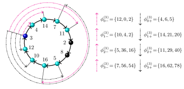
Figure 4: Illustration of the knowledge-discovery procedure: messages sent by vertex $3$ in fig: comb-cycles.

Illustrative Example. fig:knowledge-disc presents the messages sent by vertex $3$ in fig: comb-cycles during the $k^{th}$ ($1\!\leq\!k\!\leq\!4$) iteration of the knowledge-discovery procedure. For example, in the $3^{rd}$ iteration, vertex $3$ sends to vertex $11\!=\!\sigma^{4}(3)$ the knowledge set $\phi_{2-}^{(3)}\!=\!\{\sigma^{-4}(3),w_{r}(\sigma^{-4}(3)\!\leadsto\!3),w_{g}(\sigma^{-4}(3)\!\leadsto\!3)\}\!=\!\{5,36,16\}$ (the $3^{rd}$ up arrow from top to bottom in right half of fig:knowledge-disc) it learns during the $2^{nd}$ iteration. It also sends to vertex $5\!=\!\sigma^{-4}(3)$ the knowledge set $\phi_{2+}^{(3)}\!=\!\{\sigma^{4}(3),w_{r}(3\!\leadsto\!\sigma^{4}(3)),w_{g}(3\!\leadsto\!\sigma^{4}(3))\}\!=\!\{11,29,40\}$ (the $3^{rd}$ down arrow from top to bottom in right half of fig:knowledge-disc). Though it is not shown in fig:knowledge-disc, in the same iteration, vertex $3$ receives $\phi_{2+}^{(11)}=\{\sigma^{4}(11),w_{r}(11\!\leadsto\!\sigma^{4}(11)),w_{g}(11\!\leadsto\!\sigma^{4}(11))\}\!=\!\{16,33,38\}$ from vertex $11\!=\!\sigma^{4}(3)$ so that it can compute, by eq:comp-know, $\sigma^{8}(3)\!=\!16$, $w_{r}(3\!\leadsto\!\sigma^{8}(3))\!=\!w_{r}(3\!\leadsto\!\sigma^{4}(3))\!+\!w_{r}(11\!\leadsto\!\sigma^{4}(11))\!=\!29+33\!=\!62$, and $w_{g}(3\!\leadsto\!\sigma^{8}(3))\!=\!w_{g}(3\!\leadsto\!\sigma^{4}(3))\!+\!w_{g}(11\!\leadsto\!\sigma^{4}(11))\!=\!40\!+\!38\!=\!78$, which is precisely $\phi_{3+}^{(3)}$. It also receives $\phi_{2-}^{(5)}\!=\!\{\sigma^{-4}(5),w_{r}(\sigma^{-4}(5)\!\leadsto\!5),w_{g}(\sigma^{-4}(5)\!\leadsto\!5)\}$ from vertex $5=\sigma^{-4}(3)$. Similarly, it can compute $\phi_{3-}^{(3)}\!=\!\{\sigma^{-8}(3),w_{r}(\sigma^{-8}(3)\!\leadsto\!3),w_{g}(\sigma^{-8}(3)\!\leadsto\!3)\}\!=\!\{7,56,54\}$. Therefore, vertex $3$ discovers vertex $16\!=\!\sigma^{8}(3)$ and $7\!=\!\sigma^{-8}(3)$ respectively.

5.2.3 Early Halt Checking

The knowledge-discovery procedure might halt before finishing the $1\!+\!\log_{2}N$ iterations. As shown in serenade: halt-check, the procedure will halt if vertex $i$ discovers some vertex twice. More precisely, if vertex $i$ discovers the same vertex twice in the same iteration, i.e., $\sigma^{2^{k}}(i)\!=\!\sigma^{-2^{k}}(i)$ or it discovers a vertex that has been discovered in the previous iterations, i.e., vertex $i$ has already discovered $\sigma^{2^{k}}(i)$ (or $\sigma^{-2^{k}}(i)$) in the previous iterations. By fact:disc, we can conclude that vertex $i$ can make the exact same matching decision as it would under SERENA.

Halt Checking in $O(1)$ Per Iteration. Vertex $i$ can finish halt checking in $O(1)$ (per port) per iteration, or $O(\log N)$ in total, using a pointer array $B[1..N]$. Here, we only need to show that the latter case described above, i.e., checking whether vertex $i$ has already discovered $\sigma^{2^{k}}(i)$ (or $\sigma^{-2^{k}}(i)$) in the previous iterations, in $O(1)$, as the checking for the former case (i.e., whether $\sigma^{2^{k}}(i)\!=\!\sigma^{-2^{k}}(i)$) is obviously $O(1)$. Each array entry $B[i^{\prime}]$ initially points to NULL. At the end of each iteration (including the $0^{th}$ iteration), vertex $i$ simply checks whether $B[\sigma^{2^{k}}(i)]\!\neq\!\texttt{NULL}$ (or $B[\sigma^{-2^{k}}(i)]\!\neq\!\texttt{NULL}$). If so, then $\sigma^{2^{k}}(i)$ (or $\sigma^{-2^{k}}(i)$) has been discovered in the previous iterations. Otherwise, we update $B$ as follows: pointing $B[\sigma^{2^{k}}(i)]$ and $B[\sigma^{-2^{k}}(i)]$ to the knowledge set $\phi_{k+}^{(i)}$ and $\phi_{k-}^{(i)}$ respectively.

Note that we need to reset the values of all $N$ entries of $B$ to NULL at the end of a matching computation. The computational complexity of the reset is $O(\log N)$ (instead of $O(N)$) because each non-null entry of $B$ is indexed by the identity field of a knowledge set, the total number of which is upper-bounded by $2\!+\!2\log_{2}N$. Hence the total computational complexity for each vertex $i$ to finish halt checking, i.e., serenade: halt-check of alg: serenade-general, is $O(1)$ (per port) per iteration, or $O(\log N)$ in total.

All or None Lemma. Using the similar operations as in the proof of fact:disc, vertex $i$ can use $O(1)$ operations to decide which is heaver between the green weight and the red weight of the cycle that vertex $i$ belongs to. So can other vertices belonging to the same cycle (as vertex $i$) by using the following lemma.

Lemma 2 (All or None).

During the execution of the knowledge-discovery procedure in SERENADE, if any vertex $i$ halts before finishing the $1\!+\!\log_{2}N$ iterations, i.e., halting because of discovering some vertex twice in serenade: halt-check of alg: serenade-general, then all other vertices belonging to the same cycle will also halt in the same iteration

Proof:

See app:proof-of-lemma-02. ∎

5.2.4 Discussions

In describing the knowledge-discovery procedure, we assume that input ports can communicate directly with each other. This is a realistic assumption, because in most real-world switch products, each line card $i$ is full-duplex in the sense the logical input port $i$ and the logical output port $i$ are co-located in the same physical line card $i$. In this case, for example, an input port $i_{1}$ can communicate with another input port $i_{2}$ by sending information to output port $i_{2}$, which then relays it to the input port $i_{2}$ through the “local bypass”, presumably at little or no communication costs. However, SERENADE also works for the type of switches that do not have such a “local bypass,” by letting an output port to serve as a relay, albeit at twice the communication costs. More precisely, in the example above, the input port $i_{1}$ can send the information first to the output port $i_{1}$, which then relays the information to the input port $i_{2}$.

5.3 Complexity Analysis

We now analyze the time and message complexities of the knowledge-discovery procedure.

Time Complexity. The time complexity of the knowledge-discovery procedure is (at most) $1\!+\!\log_{2}N$ iterations, and that of each iteration is several operations for local computation for computing knowledge sets (Lines 1-1 of alg: serenade-general) and halt checking (serenade: halt-check of alg: serenade-general). Clearly, those operations can be performed in $O(1)$.

Message Complexity. The message complexity of the knowledge-discovery procedure is $O(\log N)$ messages per vertex, since every vertex needs to send (and receive) two messages during each iteration. In every message, it suffices to only include $w_{r}(\cdot)\!-\!w_{g}(\cdot)$, the difference between the red and the green weights of the corresponding walk. Therefore, each message (i.e., knowledge set) can be encoded in $C\!+\!\log_{2}N$ bits, where $C$ is the maximum number of bits needed to encode this difference.

5.4 Early Halt: The Ouroboros Cycles

In this section, we define the concept of an ouroboros cycle, and prove lemma:ouroboros-lemma, which states that all vertices on an ouroboros cycle can halt (serenade: halt-check of alg: serenade-general) and make the exact same matching decisions as they would under SERENA, without performing the distributed binary search. Ouroboros is the ancient Greek symbol depicting a serpent devouring its own tail. We “borrow” this concept because what happens in ouroboros cycles is very similar to what is depicted by the symbol “Ouroboros”.

Definition 2 (Ouroboros Cycle).

A cycle is said to be ouroboros if and only if its length $\ell$ is an ouroboros number (w.r.t. $N$), defined as a positive divisor of a number that takes one of the following three forms: (I) $2^{\alpha}$, (II) $2^{\beta}\!-\!2^{\gamma}$, and (III) $2^{\beta}\!+\!2^{\gamma}$, where $\alpha$, $\beta$ and $\gamma$ are nonnegative integers that satisfy $\alpha\!\leq\!\lceil\!\log_{2}N\rceil$ and $\gamma\!<\!\beta\!\leq\!\lceil\!\log_{2}N\rceil$.

It is not hard to check that, in fig: comb-cycles, the leftmost cycle (of length $11$) is not ouroboros (i.e., non-ouroboros), but the other two are.

The following lemma shows a nice property of ouroboros cycles, whose proof can be found in app:proof-of-lemma-03.

Lemma 3 (Ouroboros Lemma).

Vertex $i$ will discover twice a vertex on the same cycle (as itself) during the knowledge-discovery stage, if it is on an ouroboros cycle.

Remark. Readers may wonder if we can do away with the distributed binary search simply by running a little more iterations (say $0.5\log_{2}N$ more iterations), because more iterations means that more vertices may discover a vertex twice. Unfortunately, as shown in app:why-not-more, there exists some numbers (cycle lengths) that are “hardcore non-ouroboros” in the sense a vertex $i$ on a cycle of such a length $\ell$ needs to run exactly $\lceil\ell/2\rceil$ iterations to discover a vertex twice.

6 Leader Election

We have shown that the $1\!+\!\log_{2}N$ iterations of the knowledge-discovery procedure alone is not enough for SERENADE to emulate SERENA exactly. To do so, SERENADE needs an additional distributed binary search. As mentioned in sec: serenade, the distributed binary search requires every non-ouroboros cycle to elect a designated vertex, which is decided through a leader election by vertices on this cycle. In this section, we describe how to embed this leader election seamlessly into the knowledge-discovery procedure of SERENADE.

6.1 Leader Election

We explain this process on an arbitrary combinatorial cycle of $\sigma$, focusing on the actions of an arbitrary vertex $i$ that belongs to this cycle. We follow the standard practice [14] of making the vertex with the smallest identity (an integer between $1$ and $N$) on this cycle the leader. Recall that in the knowledge-discovery procedure, after each (say $k^{th}$) iteration, vertex $i$ discovers $\sigma^{-2^{k}}(i)$ that is “$2^{k}$ $\sigma$-hops away” from it on the cycle. More precisely, vertex $i$ learns $\phi^{(i)}_{k-}$, which contains the identities of the vertex $\sigma^{-2^{k}}(i)$, and the red and green weights of the walk $\sigma^{-2^{k}}(i)\leadsto i$. Our goal is to augment this $k^{th}$ iteration to learn the vertex with the smallest identity on this walk $\sigma^{-2^{k}}(i)\!\leadsto\!i$, which we denote as $\mathcal{L}(\sigma^{-2^{k}}(i)\!\leadsto\!i)$ and call the leader of the level-$k$ precinct right-ended at $i$.

Like in the knowledge-discovery procedure, we explain this augmentation inductively. The case of $k\!=\!0$ (i.e., the $0^{th}$ iteration) is as follows: Each vertex $i$ considers the one with smaller identity between itself and $\sigma^{-1}(i)$ to be the leader of the level-0 precinct right-ended at $i$.

For the $k^{th}$ ($k\!\geq\!1$) iteration, each vertex $i$ only needs to augment the knowledge set it sends downstream to $i_{D}\!=\!\sigma^{2^{k-1}}(i)$ with $\mathcal{L}(\sigma^{(-2^{k-1})}(i)\!\leadsto\!i)$ (the leader of the level-$(k\!-\!1)$ precinct right-ended at $i$) in serenade: send-down of alg: serenade-general. Meanwhile, it receives, from $i_{U}\!=\!\sigma^{(-2^{k-1})}(i)$, the vertex $2^{k\!-\!1}$ $\sigma$-hops upstream, $\mathcal{L}(\sigma^{(-2^{k-1})}(i_{U})\!\leadsto\!i_{U})$ (the leader of the level-$(k-1)$ precinct right-ended at $i_{U}$) in serenade: receive-up of alg: serenade-general, as $i_{U}$ also augments its knowledge set. In addition, each vertex $i$ also adds the following local computation in serenade: compute-knowledge-set-minus of alg: serenade-general.

The following lemma concerns the correctness of and the minimum number of iterations (i.e., $1\!+\!\log_{2}N$) required by the above embedded leader election. This is also the reason why we choose to execute the knowledge-discovery procedure for $1\!+\!\log_{2}N$ iterations. Its proof is straightforward, we omit it in this paper.

Lemma 4.

Given any non-ouroboros cycle, each vertex $i$ belonging to it will learn, through the augmented knowledge-discovery procedure, the identity of the leader for the cycle, after at most $1\!+\!\log_{2}N$ iterations. Besides, there exists some non-ouroboros cycle such that some of its vertices need at least $1\!+\!\log_{2}N$ iterations to learn the identity of the leader.

6.2 Distribute Leaders’ Decisions

Once the leader of a non-ouroboros cycle is decided, through a distributed binary search (to be described in subsec:bs), the leader will discover itself (through a non-empty walk). According to fact:disc, the leader now can make the same matching decision as it would under SERENA. Then, the leader informs the switch controller of its decision on whether to choose the green or the red sub-matching, and the switch controller then broadcasts decisions of all leaders to the $N$ vertices. Since each vertex on a non-ouroboros cycle knows the identity of its leader by thm:leader-election, it will follow the decision made by its leader in choosing between the red and the green sub-matchings.

The size of this broadcast, equal to the number of non-ouroboros cycles in $\sigma$, is small (with overwhelming probability). For example, we will show in subsec:message-comp that even when $N\!=\!256$, the average number of non-ouroboros cycles is no more than $1.69$ and in more than $99\%$ of instances, there are no more than $4$ non-ouroboros cycles per time slot.

1

2Procedure BinarySearch($i$, $k$, $w_{g}$, $w_{r}$)

3      

4      If $i$ (self) is $\mathcal{L}_{0}$ then halt;

5      

6      if $\sigma^{(-2^{k-1})}(i)=\mathcal{L}_{0}$ then

7            

8            $w_{g}\leftarrow w_{g}-w_{g}\big{(}\sigma^{(-2^{k-1})}(i)\leadsto i\big{)}$;

9            

10            $w_{r}\leftarrow w_{r}-w_{r}\big{(}\sigma^{(-2^{k-1})}(i)\leadsto i\big{)}$;

11            

12            BinarySearch($\mathcal{L}_{0},k\!-\!1,w_{g},w_{r}$);

13            

14      else

15            

16            if $\mathcal{L}_{0}=\mathcal{L}(\sigma^{(-2^{k-1})}(i)\leadsto i$) then

17                  

18                  BinarySearch($i$, $k-1$, $w_{g}$, $w_{r}$);

19                  

20            else

21                  

22                  $w_{g}\leftarrow w_{g}-w_{g}\big{(}\sigma^{(-2^{k-1})}(i)\leadsto i\big{)}$;

23                  

24                  $w_{r}\leftarrow w_{r}-w_{r}\big{(}\sigma^{(-2^{k-1})}(i)\leadsto i\big{)}$;

25                  

26                  BinarySearch($\sigma^{(-\!2^{k\!-\!1})}(i){,}k\!-\!1{,}w_{g}{,}w_{r}$);

27                  

28            

29      

Algorithm 2 Distributed binary search at vertex $i$.

7 Distributed Binary Search Stage

As mentioned above, only vertices on ouroboros cycles can make the exact same decisions as they would under SERENA, for vertices on non-ouroboros cycles, SERENADE needs an additional distributed binary search stage. In this section, we will describe the binary search stage focusing on an arbitrary non-ouroboros cycle.

7.1 Distributed Binary Search

Without loss of generality, we assume that $\mathcal{L}_{0}$ is the leader of, and $i$ a vertex on, this non-ouroboros cycle. The objective of this distributed algorithm is to let its leader $\mathcal{L}_{0}$ discovers itself twice by searching a repetition (i.e., other than its first occurrence as the starting point of the walk) of $\mathcal{L}_{0}$ along the walk $\mathcal{L}_{0}\!\leadsto\!\sigma^{N}(\mathcal{L}_{0})$, the level-($\log_{2}N$) precinct right-ended at $\sigma^{N}(\mathcal{L}_{0})$; this repetition must exist because $N$, the length of the walk $\mathcal{L}_{0}\leadsto\sigma^{N}(\mathcal{L}_{0})$, is no smaller than the length of this cycle. To this end, vertices on this non-ouroboros cycle perform a distributed binary search, guided by the leadership information each vertex obtains through the leader election. In the following, we describe the high-level ideas of this binary search algorithm, in which the detailed actions of a vertex $i$ are captured by alg: serenade-bsearch. Unlike the knowledge-discovery procedure, during each iteration of the distributed binary search, only one vertex on this non-ouroboros cycle performs the search task, which we call the search administrator.

High-Level Ideas. This binary search is initiated by the vertex $\sigma^{N}(\mathcal{L}_{0})$, who learns “who herself is” (i.e., that herself is $\sigma^{N}(\mathcal{L}_{0})$) during the last iteration of the augmented knowledge-discovery procedure; in other words, the initial search administrator is $\sigma^{N}(\mathcal{L}_{0})$. The initial search interval is the entire walk $\mathcal{L}_{0}\leadsto\sigma^{N}(\mathcal{L}_{0})$, also the level-$(\log_{2}N)$ precinct right-ended at $\sigma^{N}(\mathcal{L}_{0})$. The search administrator $\sigma^{N}(\mathcal{L}_{0})$ first checks whether itself or $\sigma^{N/2}(\mathcal{L}_{0})$, the middle point of the search interval, is a repetition of $\mathcal{L}_{0}$. If so, the entire search mission is accomplished, so the search ends. Otherwise, it checks whether there is a repetition of $\mathcal{L}_{0}$ in the right half of the search interval by checking whether $\mathcal{L}(\sigma^{N/2}(\mathcal{L}_{0})\leadsto\sigma^{N}(\mathcal{L}_{0}))$ is equal to $\mathcal{L}_{0}$; note the identity of $\mathcal{L}(\sigma^{N/2}(\mathcal{L}_{0})\leadsto\sigma^{N}(\mathcal{L}_{0}))$, the leader of the level-$(\log_{2}(N)-1)$ precinct right-ended at $\sigma^{N}(\mathcal{L}_{0})$, is known to $\sigma^{N}(\mathcal{L}_{0})$, since it is one of the leadership information $\sigma^{N}(\mathcal{L}_{0})$ learns through the leader election. If so, the same search administrator $\sigma^{N}(\mathcal{L}_{0})$ carries on this binary search in the right half of the search interval. Otherwise, the middle point of the search interval $\sigma^{N/2}(\mathcal{L}_{0})$ becomes the new search administrator and carries on this binary search in the left half.

Pseudocode Explanation. As mentioned above, the detailed actions of any search administrator $i$ are captured by alg: serenade-bsearch. Initially $i$ is $\sigma^{N}(\mathcal{L}_{0})$ who assigns $\log_{2}N$ to $k$, the $2^{nd}$ argument of alg: serenade-bsearch, which indicates the search interval is $\sigma^{-2^{k}}\!\leadsto\!i$. To ensure that $\mathcal{L}_{0}$ can discover itself, i.e., learning the green and red weights of a non-empty walk from $\mathcal{L}_{0}$ to itself, search administrator $i$ also maintains the weight information $w_{g}$, $w_{r}$ (the $3^{rd}$ and $4^{th}$ arguments of alg: serenade-bsearch), which are the green and red weights of the walk from $\mathcal{L}_{0}$ to $i$. Initially, search administrator $\sigma^{N}(\mathcal{L}_{0})$ knows the green and red weights of the walk $\mathcal{L}_{0}\!\leadsto\!\sigma^{N}(\mathcal{L}_{0})$, because they belong to the knowledge sets that $\sigma^{N}(\mathcal{L}_{0})$ learns during the last iteration of the augmented knowledge-discovery procedure. We will not describe alg: serenade-bsearch line-by-line, since the actions of search administrator $i$ are the same as those of the initial search administrator we described above, except that alg: serenade-bsearch details the operations for bookkeeping weight information.

The correctness of the distributed binary search and the number of iterations it requires, which are summarized in the following lemma, can be proved with mathematical induction. Here, we omit it for brevity.

Lemma 5.

Given any non-ouroboros cycle with a length of $\ell$, the distributed binary search enables the leader $\mathcal{L}_{0}$ of this cycle to discover itself twice with at most $\lceil\log_{2}\ell\rceil$ iterations.

7.2 Complexity Analysis

In this section, we analyze the time and message complexities of the distributed binary search.

Time Complexity. The time complexity (i.e., number of iterations) of the distributed binary search is upper-bounded by $\lceil\log_{2}\eta\rceil$ ($\leq\!\log_{2}N$) iterations, where $\eta$ is the length of the longest non-ouroboros cycle, since binary searches at different non-ouroboros cycles are performed simultaneously. Hence, it can be as large as $\log_{2}N$ iterations, each of which contains roughly $3$ operations ($2$ additions and $1$ comparison), in the worst case.

Message Complexity. As explained in subsubsec: b-search, during the binary search, on each non-ouroboros cycle a message (to maintaining the weight information) is transmitted only when the search administrator moves from one vertex to another, so the message complexity of the binary search, in the worst-case, is at most $1$ message per vertex. Each message needs $\lceil\log_{2}\log_{2}N\rceil\!+\!C$ bits, where $C$ is the number of bits for encoding $w_{r}(\cdot)\!-\!w_{g}(\cdot)$.

8 Early Stop: O-SERENADE

In this section, we present an early-stop version of SERENADE to approximately emulate SERENA, without performing the distributed binary search, in which vertices on any non-ouroboros cycle make a decision based on the (insufficient) information at hand after the augmented knowledge-discovery procedure. As will be shown in sec:evaluation, O-SERENADE trades no degradation of delay performances for significant reduction in time complexities (i.e., without performing the distributed binary search that has up to $\log_{2}N$ iterations).

Decision Rule. Now we describe the decision rule of this early-stop version in an arbitrary non-ouroboros cycle. The decision rule is for the leader $\mathcal{L}_{0}$ of this cycle to compare the green and the red weights of the longest such walk $\mathcal{L}_{0}\!\leadsto\!\sigma^{N}(\mathcal{L}_{0})$, and pick, on behalf of the whole cycle, the green or the red sub-matching according to the outcome of this comparison; note we cannot simply let every vertex $i$ on this cycle to pick the green or the red edge individually based on its local view of $w_{r}\big{(}i\leadsto\sigma^{N}(i)\big{)}$ vs. $w_{g}\big{(}i\leadsto\sigma^{N}(i)\big{)}$, since these local views can be inconsistent. For example, for the leftmost cycle in fig: comb-cycles, it is not hard to check vertex $2$ and vertex $3$ have inconsistent local views: $w_{g}\big{(}2\!\leadsto\!\sigma^{16}(2)\big{)}\!=\!120\!<\!134\!=\!w_{r}\big{(}2\!\leadsto\!\sigma^{16}(2)\big{)}$ (vertex $2$’s local view) and $w_{g}\big{(}3\!\leadsto\sigma^{16}(3)\!\big{)}\!=\!130\!>\!112\!=\!w_{r}\big{(}3\!\leadsto\sigma^{16}(3)\!\big{)}$ (vertex $3$’s local view). It is clear that O-SERENADE will pick the red sub-matching in this cycle based on the local view of its leader (i.e., vertex $2$), which is different from the decision under SERENA. This strategy is opportunistic as it does not hesitate to pick a sub-matching that appears to be larger, even though there is a small chance this appearance is incorrect. Therefore, we call it O-SERENADE. Like SERENADE, this early-stop version also needs the switch controller to broadcast the decisions of all the leaders to the $N$ vertices.

Rationale. The rationale behind the opportunistic strategy is as follows. When the weight difference between the red and the green sub-matchings is small, it matters little which sub-matching is picked. When the difference is large, however, this strategy likely will further inflate the already large difference and hence result in the correct sub-matching being picked.

9 Performance Evaluation

In this section, we evaluate, through simulations, the throughput and delay performances of O-SERENADE under various load conditions and traffic patterns to be specified in subsec: sim-setting; there is no need to evaluate the throughput and delay performances of SERENADE, which exactly emulates SERENA. Note that we have also evaluated the message complexity of SERENADE, and investigated how the mean delay performance of O-SERENADE scales with respect to N, the number of (input/output) ports; these results can be found in app:more-sim.

9.1 Simulation Setup

In all our simulations, the number of input/output ports $N$ is $64$, unless otherwise stated. To measure throughput and delay accurately, we assume each VOQ has an infinite buffer size and hence there is no packet drop at any input port. Every simulation run lasts $30,000\times N^{2}$ time slots. This duration is chosen so that every simulation run enters the steady state after a tiny fraction of this duration and stays there for the rest. The throughput and delay measurements are taken after the simulation run enters the steady state.

Like in [8], we assume, in the following simulations, that the traffic arrival processes to different input ports are mutually independent, and each such arrival process is i.i.d. Bernoulli (i.e., at any given input port, a packet arrives with a constant probability $\rho\in(0,1)$ during each time slot). Note that we only use synthetic traffic (instead of that derived from packet traces) because, to the best of our knowledge, there is no meaningful way to combine packet traces into switch-wide traffic workloads. The following $4$ standard types of load matrices (i.e., traffic patterns) are used to generate the workloads of the switch: (I) Uniform: packets arriving at any input port go to each output port with probability $\frac{1}{N}$. (II) Quasi-diagonal: packets arriving at input port $i$ go to output port $j\!=\!i$ with probability $\frac{1}{2}$ and go to any other output port with probability $\frac{1}{2(N-1)}$. (III) Log-diagonal: packets arriving at input port $i$ go to output port $j=i$ with probability $\frac{2^{(N-1)}}{2^{N}-1}$ and go to any other output port $j$ with probability equal $\frac{1}{2}$ of the probability of output port $j-1$ (note: output port $0$ equals output port $N$). (IV) Diagonal: packets arriving at input port $i$ go to output port $j\!=\!i$ with probability $\frac{2}{3}$, or go to output port $(i\,\text{mod}\,N)+1$ with probability $\frac{1}{3}$.

The load matrices are listed in order of how skewed the traffic volumes to different output ports are: from uniform being the least skewed, to diagonal being the most skewed. Finally, we emphasize that, every non-zero diagonal element (i.e., traffic from an input port $i$ and an output port $i$), in every traffic matrix we simulated on, is actually switched by the crossbar and consumes just as much switching resources per packet as other traffic matrix elements, and never takes advantage of the “local bypass” (see subsubsec: logical_bypass) that may exist between the input port $i$ and the output port $i$.

9.2 Throughput Performance

Our simulation results show that O-SERENADE can achieve $100\%$ throughput under all $4$ load matrices and i.i.d. Bernoulli traffic arrivals: The VOQ lengths remain stable under an offered load of $0.99$ in all these simulations.

9.3 Delay Performance

Now we shift our focus to the delay performance of O-SERENADE. We compare its delay performance only with that of SERENA and MWM. We refer readers to [8] for comparisons between SERENA and some other crossbar scheduling algorithms such as iSLIP [10] and iLQF [15].

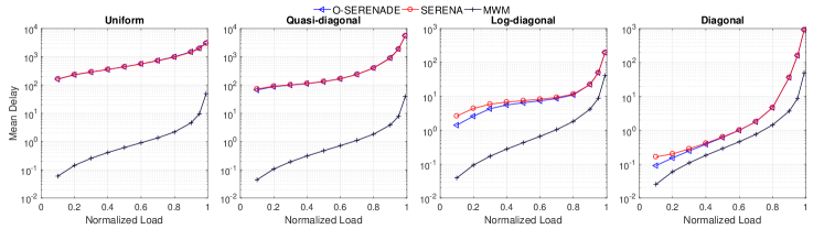
Figure 5: Mean delays of O-SERENADE, SERENA and MWM under the $4$ traffic load matrices.

O-SERENADE vs. SERENA.  fig: delay-vs-loadsO shows the mean delays of the three algorithms under the $4$ traffic load matrices above respectively. Each subfigure shows how the mean delays (on a log scale along the y-axis) vary with different offered loads (along the x-axis). fig: delay-vs-loadsO shows that overall O-SERENADE and SERENA perform similarly under all $4$ traffic load matrices and all load factors. Upon observing these simulation results, our interpretation was that the decisions made by O-SERENADE agree with the ground truth (i.e., which sub-matching is indeed heavier on a non-ouroboros cycle) most of time. This interpretation was later confirmed by further simulations: They agree in between $90.57\%$ and $99.99\%$ of the instances.

Perhaps surprisingly, fig: delay-vs-loadsO also shows that O-SERENADE performs slightly better than SERENA when the traffic load is low (say $<0.4$) under log-diagonal and diagonal traffic load matrices. Our interpretation of this observation is as follows. It is not hard to verify that decisions made by O-SERENADE can disagree with the ground truth, with a non-negligible probability, only when the total green and the total red weights of a non-ouroboros cycle are very close to one another. However, in such cases, picking the wrong sub-matchings (i.e., disagreeing with the ground truth) causes almost no damages. Furthermore, we speculate that it may even help O-SERENADE jump out of a local maximum (i.e., have the effect of simulated annealing) and converge more quickly to a near-optimal matching (in terms of weight), thus resulting in even better delay performance.

10 Related Work

In the interest of space, we provide only a brief survey of the prior art that is directly related to our work. Since SERENADE parallelizes SERENA, which computes approximate Maximum Weight Matching (MWM), we focus mostly on the following two categories: (1) parallel or distributed algorithms for exact or approximate MWM computation with applications to crossbar scheduling (in subsec: sched-alg-crossbar) and (2) distributed matching algorithms with applications to transmission scheduling in wireless networks (in subsec: sched-alg-wireless). In particular, we will keep to a minimum the comparisons between SERENA and other sequential crossbar scheduling algorithms proposed before SERENA, of which a thorough survey was provided in [8].

A few sequential crossbar scheduling algorithms were proposed [11, 16]. However, none of these algorithms beats SERENA in both (delay and throughput) performance and computational complexity under the standard problem setting (e.g., fixed packet size). A template that can be instantiated into a family of throughput-optimal algorithms for scheduling crossbar or wireless transmission, and a unified framework for proving the throughput-optimality of all these algorithms were proposed in [17, 18]. The only crossbar scheduling algorithm that results from this template is the instantiation of a BP-based MWM algorithm [19], which has a message and time complexity of $O(N)$ per port. In [20], an efficient distributed iterative algorithm, called RR/LQF, was proposed. Although its computational complexity can be as low as one iteration (but at a cost), and its message complexity as low as one bit per port, it requires a crossbar speedup of $2-1/N$ to achieve $100\%$ throughput, if it runs $N$ iterations of the algorithm, where $N$ is the number of input/output ports. Recently, an “add-on” algorithm called Queue-Proportional Sampling (QPS) was proposed in [21] that can be used to augment, and boost the delay performance of, SERENA [8]. However, the resulting QPS-SERENA has the same $O(N)$ time complexity as SERENA.

In all algorithms above, a matching decision is made every time slot. An alternative type of algorithms is frame-based  [22, 23, 24, 25, 26], in which multiple (say $K$) consecutive time slots are grouped as a frame. These $K$ matching decisions in a frame are batch-computed, which usually has lower time complexity than $K$ independent matching computations. However, since $K$ is usually quite large (e.g., $K\!=\!O(\log N)$), and a packet arriving at the beginning of a frame has to wait till at least the beginning of the next frame to be switched, frame-based scheduling generally results in higher queueing delays.

10.1 Parallel/Distributed MWM Algorithms

As mentioned earlier, MWM is the ideal crossbar scheduling policy in the sense that it can achieve 100% throughput and that it has delay performance conjectured to be optimal, but its most efficient implementation [6] has a prohibitively high computational complexity of $O(N^{3})$. This dilemma has motivated the development of a few parallel or distributed algorithms that, by distributing this computational cost across multiple processors (nodes), bring down the per-node computational complexity.

The most representative among them are [27, 28, 19, 29]. A parallel algorithm with a sub-linear per-node computational complexity of $O(\sqrt{N}\log^{2}N)$ was proposed in [27] for computing MWM exactly in a bipartite graph. However, this algorithm requires the use of $O(N^{3})$ processors. Another two [28, 19] belong to the family of distributed iterative algorithms based on belief-propagation (BP). In this family, the input ports engage in multiple iterations of message exchanges with the output ports to learn enough information about the lengths of all $N^{2}$ VOQs so that each input port can decide on a distinct output port to match with. The resulting matching either is, or is close to, the MWM. Note that the BP-based algorithms are simply parallel algorithms to compute the MWM: the total amount of computation, or the total number of messages needed to be exchanged, is still $O(N^{3})$, but is distributed evenly across the input and the output ports (i.e., $O(N^{2})$ work for each input/output port). It was shown in [29] that BP can also be used to boost the performance of other (non-BP-based) distributed iterative algorithms such as iLQF [15]. However, the “BP assistance” part alone has a total computational complexity of $O(N^{2})$, or $O(N)$ per port.

10.2 Wireless Transmission Scheduling

Transmission scheduling in wireless networks with primary interference constraints [30] shares a common algorithmic problem with crossbar scheduling: to compute a good matching for each “time slot”. The matching computation in the former case is however more challenging, since it needs to be performed over a general graph that is not necessarily bipartite. Several wireless transmission scheduling solutions were proposed in the literature [31, 30, 32, 33, 34, 35] that are based on distributed computation of matchings in a general graph.

Most of these solutions tackle the underlying distributed matching computation problem using an adaptation/extension of either [36] (used in [34, 33, 35]), or [37] (used in [32, 31]). In [36], a parallel randomized algorithm was proposed that outputs a maximal matching with expected runtime $O(\log|E|)$, where $|E|$ is the number of edges in the graph. This computational complexity, translated into our crossbar scheduling context, is $O(\log N)$. However, maximal matching algorithms are known to only guarantee at least $50\%$ throughput [4]. The work of Hoepman [37] converts an earlier sequential algorithm for computing approximate MWM [38] to a distributed one. However, the distributed algorithm in [37], like its sequential version [38], can only guarantee to find a matching whose weight is at least half of that of the MWM, and hence can only guarantee at least $50\%$ throughput also. In comparison, SERENADE guarantees $100\%$ throughput, just like its sequential version SERENA.

The only exception, to distributed matching algorithms being based on either [36] or [37], is [30], in which the scheduling algorithm, called MIX, is a distributed version of the MERGE procedure in SERENA, albeit in the wireless networking context. The objective of MIX is to compute an approximate MWM for simultaneous non-interfering wireless transmissions of packets, where the weight of a directed edge (say a wireless link from a node $X$ to a node $Y$) is the length of the VOQ at $X$ for packets destined for $Y$, in the SERENA manner: MERGE the matching used in the previous time slot with a new random matching. Unlike in SERENA, however, neither matching has to be full and the connectivity topology is generally not bipartite in a wireless network, and hence the graph resulting from the union of the two matchings can contain both cycles and paths.

MIX has three variants. As we will explain in subsec: serenade-vs-gossiping in details, all three variants compute the total – or equivalently the average – green and red weights of each cycle or path either by linearly traversing the cycle or path, or via a gossip algorithm [39]; they all try to mimic SERENA in a wireless network and have a time complexity at least $O(N)$, as compared to $O(\log N)$ for SERENADE. To summarize, they are clearly all “wireless SERENA”, not “wireless SERENADE”.

11 Conclusion

In this paper, we propose SERENADE, a parallel iterative algorithm that can provably, with a time complexity of only $O(\log N)$ per port, exactly emulate SERENA, a centralized algorithm with $O(N)$ time complexity. We also propose an early-stop version of SERENADE, called O-SERENADE, which only approximately emulates SERENA. Through extensive simulations, we demonstrate that O-SERENADE can achieve $100\%$ throughput. We also demonstrate that O-SERENADE has delay performances either similar as or better than those of SERENA, under various load conditions and traffic patterns.

Appendix A Parallelized Population

As explained in sec: serena-and-merge, the new random matching $A^{\prime}(t)$ derived from the arrival graph, which is in general a partial matching, has to be populated into a full matching $R(t)$ before it can be merged with $S(t-1)$, the matching used in the previous time slot. SERENADE parallelizes this POPULATE procedure, i.e., the round-robin pairing of unmatched input ports in $R(t)$ with unmatched output ports in $R(t)$, so that the computational complexity for each input port is $O(\log N)$, as follows.

Suppose that each unmatched port (input port or output port) knows its own ranking, i.e., the number of unmatched ports up to itself (including itself) from the first one (we will show later how each unmatched port can obtain its own ranking). Then, each unmatched input port needs to obtain the identity of the unmatched output port with the same ranking. This can be done via $3$ message exchanges as follows. Each pair of unmatched input and output ports “exchange” their identities through a “broker”. More precisely, the $j^{th}$ unmatched input port (i.e., unmatched input port with ranking $j$) first sends its identity to input port $j$ (i.e., the broker). Then, the $j^{th}$ unmatched output port also sends its identity to input port $j$ (i.e., the broker). Finally, input port $j$ (i.e., the broker) sends the identity of the output port with ranking $j$ to the input port (with ranking $j$). Thus, the input port learns the identity of the corresponding output port. Note that, since every pair of unmatched input port and output port has its unique ranking, thus they would have different “brokers”. Therefore, all pairs can simultaneously exchange their messages without causing any congestion (i.e., a port sending or receiving too many messages).

It remains to parallelize the computation of ranking each port (input port or output port). This problem can be reduced to the parallel prefix sum problem [40] as follows. Here, we will only show how to compute the rankings of input ports in parallel; that for output ports is identical. Let $B[1..N]$ be a bitmap that indicates whether input port $i$ is unmatched (when $B[i]=1$) or not (when $B[i]=0$). Note that, this bitmap is distributed, that is, each input port $i$ only has a single bit $B[i]$. For $i=1,2,\cdots,N$, denote as $r_{i}$ the ranking of input port $i$. It is clear that $r_{i}=\sum_{k=1}^{i}B[k]$, for any $1\leq i\leq N$. In other words, the $N$ terms $r_{1}$, $r_{2}$, $\cdots$, $r_{N}$ are the prefix sums of the $N$ terms $B[1]$, $B[2]$, $\cdots$, $B[N]$. Using the Ladner-Fischer parallel prefix-sum algorithm [12], we can obtain these $N$ prefix sums $r_{1}$, $r_{2}$, $\cdots$, $r_{N}$ in $O(\log N)$ time (per port) using $2N$ processors (one at each input or output port).

Appendix B Proofs

B.1 Proof of lemma:disc

We need only to consider the following two cases.

1. The two walks are in the same “rotational” direction. Without loss of generality, we assume the two walks are $i\!\leadsto\!\sigma^{\beta}(i)$ and $i\!\leadsto\!\sigma^{\gamma}(i)$ respectively, where $0\!\leq\!\beta\!<\!\gamma$, and $\sigma^{\beta}(i)\!=\!\sigma^{\gamma}(i)\!=\!j$. By applying the operator $\sigma^{-\beta}$ to both sides of the equation $\sigma^{\beta}(i)\!=\!\sigma^{\gamma}(i)$, we have $i\!=\!\sigma^{\gamma\!-\!\beta}(i)$. Hence, $\ell$ divides ($\gamma\!-\!\beta$), where $\ell$ is the length of the cycle to which vertices $i,j$ belong. Suppose $\kappa\ell\!=\!\gamma\!-\!\beta$, where $\kappa\!>\!0$ is an integer. Then, we have the ($\gamma\!-\!\beta$)-edge-long walk $\sigma^{\beta}(i)\!\leadsto\!\sigma^{\gamma}(i)$ coils around the cycle (of length $\ell$) exactly $\kappa$ times, and so the green weight $w_{g}\big{(}\sigma^{\beta}(i)\!\leadsto\!\sigma^{\gamma}(i)\big{)}$ (or red weight) is $\kappa$ times of that of the cycle. Since vertex $i$ can obtain the green weight (or the red weight) of the walk $\sigma^{\beta}(i)\!\leadsto\!\sigma^{\gamma}(i)$ via subtracting $w_{g}(i\!\leadsto\!\sigma^{\beta}(i))$ from $w_{g}(i\!\leadsto\!\sigma^{\gamma}(i))$, i.e.,

   it knows whether $w_{g}(i\!\leadsto\!\sigma^{\ell}(i))$ (the green weight of the cycle) or $w_{r}(i\!\leadsto\!\sigma^{\ell}(i))$ (the red weight of the cycle) is larger.

2. The two walks are in opposite directions. Without loss of generality, we assume the two walks are $\sigma^{-\beta}(i)\!\leadsto\!i$ and $i\!\leadsto\!\sigma^{\gamma}(i)$ respectively where $\beta,\gamma\!>\!0$, and $\sigma^{-\beta}(i)\!=\!\sigma^{\gamma}(i)\!=\!j$. By applying the operator $\sigma^{\beta}$ to both sides of the equation $\sigma^{-\beta}(i)\!=\!\sigma^{\gamma}(i)$, we have $i\!=\!\sigma^{\gamma+\beta}(i)$. So $\ell$ divides ($\gamma\!+\!\beta$), the rest reasoning is the same as before.

B.2 Proof of lemma:all-or-nothing

Suppose that vertex $i$ discovers vertex $j$ after the $k_{1}^{th}$ and $k_{2}^{th}$ iteration respectively. Then we have $\sigma^{m_{1}}(i)\!=\!\sigma^{m_{2}}(i)\!=\!j$ where $m_{1}\!=\!2^{k_{1}}$ if $i$ discovers $j$ through serenade: compute-knowledge-set during the $k_{1}^{th}$ iteration, otherwise $m_{1}\!=\!-2^{k_{1}}$. Similarly, $m_{2}\!=\!\pm 2^{k_{2}}$. Thus, we have $i\!=\!\sigma^{m_{2}-m_{1}}(i)$. Therefore, there exists some positive integer $\kappa$ such that $\lvert m_{2}-m_{1}\rvert\!=\!\kappa\ell$, where $\ell$ is the length of the cycle.

For any other vertex $x$ on the same cycle, we have $x\!=\!\sigma^{m_{2}-m_{1}}(x)$. Thus, $\sigma^{m_{2}}(x)\!=\!\sigma^{m_{1}}(x)\triangleq y$. Therefore, $x$ also discovers $y$ twice.

B.3 Proof of lemma:ouroboros-lemma

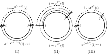
Figure 6: Illustration of three cases corresponding to cycle lengths belonging to the three forms of the ouroboros numbers.

Here we only show the proof sketch for brevity. It is not hard to show that if the cycle, to which vertex $i$ belongs, has a length of an ouroboros number, i.e., a divisor of numbers in the three forms defined in def: ouroboros-cycle, then vertex $i$ will discover a vertex $j$ on the same cycle twice via one of the three cases illustrated in fig:ouroboros-numbers. For example, if the cycle length $\ell$ is a divisor of form (I) defined in def: ouroboros-cycle, then it has to be a power of $2$. Without loss of generality, we assume $\ell\!=\!2^{\alpha}$, where nonnegative integer $\alpha\!\leq\!\log_{2}N$. In the cases of $\alpha\geq 1$, it is clear that, in the $(\alpha\!-\!1)^{th}$ iteration, vertex $i$ discovers $\sigma^{2^{\alpha\!-\!1}}(i)$ and $\sigma^{(-2^{\alpha\!-\!1})}(i)$, which turn out to be the same vertex. The case of $\alpha\!=\!0$ is slightly different: After the $0^{th}$ iteration, vertex $i$ discovers $\sigma(i)$ and $\sigma^{-1}(i)$, which are both equal to $i$. Therefore, (I) shown in fig:ouroboros-numbers happens. Similarly, we can show that if the cycle length $\ell$ is a divisor of a number in form (II) (or (III)), then (II) (or (III)) shown in fig:ouroboros-numbers happens.

Note that for (II) and (III) in fig:ouroboros-numbers, both the two walks can coil around the cycle for one or more times, and the directions of the two walks can be reversed. For example, for (III) in fig:ouroboros-numbers, the two walks could also be $\sigma^{-2^{\gamma}}(i)\!\leadsto\!i$ and $i\!\leadsto\!\sigma^{2^{\beta}}(i)$, and both of them could coil around the cycle for one or more times, i.e., they are longer than the cycle.

Appendix C Why Not Use More Than $1+\log_{2}N$ Iterations?

Fix a vertex $i$. Note that in the knowledge-discovery procedure, each iteration results in two new vertices being discovered by vertex $i$ and hence increases the chance of a vertex being discovered twice by $i$. Hence, if we run more than $1\!+\!\log_{2}N$ iterations, then vertex $i$ may discover a vertex twice even if it is on a non-ouroboros cycle (as defined in def: ouroboros-cycle). In other words, with additional iterations, some non-ouroboros numbers may become “effective ouroboros numbers”. Readers may wonder if we can do away with the distributed binary search simply by running a little more iterations (say $0.5\log_{2}N$ more iterations). Unfortunately, as shown in tab:max-iter, there exists some numbers (cycle lengths) that are “hardcore non-ouroboros” in the sense a vertex $i$ on a cycle of such a length $\ell$ needs to run exactly $\lceil\ell/2\rceil$ iterations to discover a vertex twice. In fact, it is a long-standing open problem in mathematics whether there exists infinite number of what we call “hardcore non-ouroboros” numbers here. More precisely, it is a special case of the Artin’s Conjecture [41], which, if put into our context, asks whether there are infinitely many prime numbers $p$ such that, it takes a vertex $i$ on a cycle of length $p$ exactly $\lceil p/2\rceil$ iterations to discover a vertex on the same cycle twice.

TABLE I: Examples of “hardcore non-ouroboros” numbers.

$\ell$	61	131	239	509	1019
Iterations	31	66	120	255	510

Appendix D SERENADE vs. MIX

In this section, we describe the three variants of MIX [30] in detail. The first variant, which is centralized and idealized, computes the total green and red weights of each cycle or path by “linearly” traversing the cycle or path. Hence it has a time complexity of $O(N)$, where $N$ is the number of nodes in a wireless network. This idealized variant is however impractical because it requires the complete knowledge of the connectivity topology of the wireless network.

The second variant removes this infeasible requirement and hence is practical. It estimates and compares the average green and red weights of each cycle or path (equivalent to comparing the total green and red weights) using a synchronous iterative gossip algorithm proposed in [39]. In this gossip algorithm, each node (say $X$) is assigned a green (or red) weight that is equal to the weight of the edge that uses $X$ as an endpoint and belongs to the matching used in the previous time slot (or in the new random matching); in each iteration, each node attempts to pair with a random neighbor and, if this attempt is successful, both nodes will be assigned the same red (or green) weight equal to the average of their current red (or green) weights. The time complexity of each MERGE is $O(l^{2}N\log N)$, since this gossip algorithm requires $O(l^{2}N\log N)$ iterations [30] for the average red (or green) weight estimate to be close to the actual average with high probability. Here $l$ is the length of the longest path or cycle.

The third (practical) variant, also a gossip-based algorithm, employs the aforementioned “idempotent trick” (see subsubsec: idempotent) to estimate and compare the total green and red weights of each cycle or path. This idempotent trick reduces the convergence time (towards the actual total weights) to $O(l)$ iterations, but as mentioned earlier requires each pair of neighbors to exchange a large number ($O(N\log N)$ to be exact) of exponential random variables during each message exchange. Since $l$ is usually $O(N)$ in a random graph, the time complexity of this algorithm can be considered $O(N)$.

Appendix E An Idempotent Trick

As mentioned in subsec: serenade-vs-gossiping, there is an alternative solution to the consistency problem that does not require leader election, using a standard “idempotent trick” that was used in [30] to solve a similar problem. To motivate this trick, we zoom in on the example shown in fig: comb-cycles. Both the consistency problem and the absolute correctness problem above can be attributed to the fact that the (green or red) weights of some edges are accounted for (i.e., added to the total) $\kappa$ times, while those of others $\kappa-1$ times. For example, in $3\leadsto\sigma^{16}(3)$, the (green or red) weights of edges $(3,4)$, $(4,14)$, and etc are accounted for $2$ times, while those of edges $(2,8)$, $(8,5)$, and etc $1$ times. Since the “+” operator is not idempotent (so adding a number to a counter $\kappa$ times is not the same as adding it $\kappa-1$ times), the total (green or red) weight of the walk obtained this way does not perfectly track that of the cycle.

The “idempotent trick” is to use, instead of the “+” operator, a different and idempotent operator $MIN$ to arrive at an estimation of the total green (or red) weight; the $MIN$ is idempotent in the sense the minimum of a multi-set (of real numbers) $M$ is the same as that of the set of distinct values in $M$. The idempotent trick works, in this O-SERENADE context, for a set of edges $e_{1}$, $e_{2}$, …, $e_{Z}$ that comprise a non-ouroboros cycle with green weights $w_{1}$, $w_{2}$, …, $w_{Z}$ respectively, as follows; the trick works in the same way for the red weights. Each edge $e_{\zeta}$ “modulates” its green weight $w_{\zeta}$ onto an exponential random variable $X_{\zeta}$ with distribution $F(x)=1-e^{-x/w_{\zeta}}$ (for $x>0$) so that $E[X_{\zeta}]=w_{\zeta}$. Then the green weight of every walk $W$ on this non-ouroboros cycle can be encoded as $MIN\{X_{\zeta}|e_{\zeta}\in W\}$. It is not hard to show that we can compute this MIN encoding of every $2^{d}$-edge-long walk $i\leadsto\sigma^{2^{d}}(i)$ by SERENADE-common in the same inductive way we compute the “+” encoding. For example, under the MIN encoding, serenade: send-up in alg: serenade-general becomes “Send to $i_{U}$ the value $MIN\{X_{\zeta}|e_{\zeta}\in i\leadsto\sigma^{2^{k-1}}(i)\}$”. However, unlike the “+” encoding, which requires the inclusion of only 1 “codeword” in each message, the MIN encoding requires the inclusion of $O(N\log N)$ i.i.d. “codewords” in each message in order to ensure sufficient estimation accuracy [30].

Appendix F More Simulation Results

TABLE II: Average per-port message complexities of SERENADE (bytes).

Traffic patterns		Uniform				Quasi-diagonal				Log-diagonal				Diagonal
N		64	128	256		64	128	256		64	128	256		64	128	256
light ($\rho=0.1$)		29.79	40.04	51.29		25.86	36.2	47.7		12.47	14.32	16.23		8.14	9.03	9.98
moderate ($\rho=0.6$)		34.79	44.84	55.73		31.08	40.55	50.82		21.61	25.69	29.86		14.51	16.82	19.37
high ($\rho=0.95$)		35.21	45.26	56.13		28.65	37.19	46.50		20.07	23.66	27.47		15.70	18.38	21.50

F.1 Message Complexities

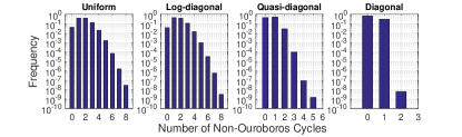
Figure 7: Histogram for number of non-ouroboros cycles in SERENADE ($N\!=\!256$, $\rho\!=\!0.6$).

In this section, we investigate the empirical message complexities of SERENADE. In the interest of space, those of O-SERENADE are not presented here, as they are similar.

Per-Port Message Complexities. tab:message-comp shows the numerical results of the average per-port message complexities (in bytes) of SERENADE for $N\!=\!$ 64, 128, and 256 for the $4$ traffic load matrices described above under low, moderate, and high offered loads. As explained in subsec: complexity-common, it suffices to only include $w_{r}(\cdot)\!-\!w_{g}(\cdot)$, the difference between the red and green weights, in each message. This difference can be encoded in $15$ bits (with a single “sign” bit), as we assume that each weight can fit in $14$ bits (i.e., no more than 16,384 packets). The worst-cast message complexities of SERENADE, described in subsec: complexity-common and subsubsec:comp-bs, are $44.25,53.25,63$ bytes per port for $N\!=\!$ 64, 128, and 256 respectively. Comparing them against those values in tab:message-comp, we can see that the average message complexities (per port), under all load factors or traffic patterns, are lower than the worst cases.

Number of Non-Ouroboros Cycles. We also measure the number of non-ouroboros cycles in each time slot in SERENADE, of which the histograms (on a log scale along the y-axis) for $N\!=\!$ 256, and an offered load of $\rho\!=\!0.6$ under the four different load matrices are shown in fig:hist-non-o. The average numbers of non-ouroboros cycles are $1.69,1.61,0.57,0.31$ under the uniform, quasi-diagonal, log-diagonal, and diagonal load matrices respectively. It is not hard to check that under any of the four different load matrices, in more than $99\%$ of instances, there are no more than $4$ non-ouroboros cycles per time slot.

F.2 Delay versus Number of Ports

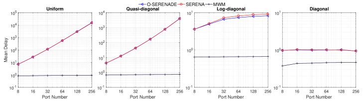
(a) Under the offered load of 0.6.

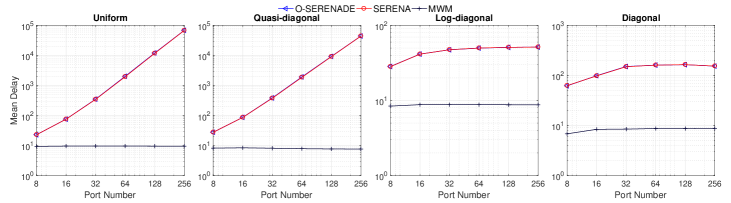
(b) Under the offered load of 0.95.

Figure 8: Mean delays v.s. port numbers under i.i.d. Bernoulli traffic arrivals with the $4$ traffic load matrices.

In this section, we investigate how the mean delay of O-SERENADE scales with the number of input/output ports $N$ under i.i.d. Bernoulli traffic. We have simulated the following different $N$ values: $N\!=\!8,16,32,64,128,256$. fig: mean-delay-vs-port-number compares the mean delays for O-SERENADE against that for SERENA under the $4$ different traffic load matrices with a moderate offered load of $0.6$ and a heavy offered load of $0.95$. As a benchmark, we also show those of MWM. It shows that the scaling behaviors of O-SERENADE are almost the same as that of SERENA in terms of mean delays, for all values of $N$. More precisely, under the log-diagonal and the diagonal load matrices, O-SERENADE achieves near-optimal scaling (i.e., nearly constant independent of $N$) of mean delay, whereas under the uniform and quasi-diagonal load matrices, the mean delay grows roughly quadratically with $N$ (i.e., $O(N^{2})$ scaling).

References

- [1] C. Cakir, R. Ho, J. Lexau, and K. Mai, “Scalable high-radix modular crossbar switches,” in Proc. of the IEEE HOTI, pp. 37–44, Aug 2016.
- [2] Y. Dai, K. Wang, G. Qu, L. Xiao, D. Dong, and X. Qi, “A scalable and resilient microarchitecture based on multiport binding for high-radix router design,” in Proc. of the IEEE IPDPS, pp. 429–438, May 2017.
- [3] M. Karol, M. Hluchyj, and S. Morgan, “Input Versus Output Queueing on a Space-Division Packet Switch,” IEEE Trans. Commun., vol. 35, pp. 1347–1356, Dec. 1987.
- [4] N. McKeown, A. Mekkittikul, V. Anantharam, and J. Walrand, “Achieving 100% Throughput in an Input-Queued Switch,” IEEE Trans. Commun., vol. 47, pp. 1260–1267, Aug. 1999.
- [5] D. Shah and D. Wischik, “Optimal Scheduling Algorithms for Input-Queued Switches,” in Proc. of the IEEE INFOCOM, pp. 1–11, Apr. 2006.
- [6] J. Edmonds and R. M. Karp, “Theoretical Improvements in Algorithmic Efficiency for Network Flow Problems,” J. ACM, vol. 19, pp. 248–264, Apr. 1972.
- [7] D. Shah, P. Giaccone, and B. Prabhakar, “Efficient Randomized Algorithms for Input-Queued Switch Scheduling,” IEEE Micro, vol. 22, pp. 10–18, Jan. 2002.
- [8] P. Giaccone, B. Prabhakar, and D. Shah, “Randomized Scheduling Algorithms for High-Aggregate Bandwidth Switches,” IEEE J. Sel. Areas Commun., vol. 21, pp. 546–559, May 2003.
- [9] A. Mekkittikul and N. McKeown, “A Practical Scheduling Algorithm to Achieve 100% Throughput in Input-Queued Switches,” in Proc. of the IEEE INFOCOM, pp. 792–799 vol.2, Mar. 1998.
- [10] N. McKeown, “The iSLIP Scheduling Algorithm for Input-queued Switches,” IEEE/ACM Trans. Netw., vol. 7, pp. 188–201, Apr. 1999.
- [11] G. R. Gupta, S. Sanghavi, and N. B. Shroff, “Node Weighted Scheduling,” in Proc. of the ACM SIGMETRICS, pp. 97–108, Jun. 2009.
- [12] R. E. Ladner and M. J. Fischer, “Parallel Prefix Computation,” J. ACM, vol. 27, pp. 831–838, Oct 1980.
- [13] N. A. Lynch, Distributed Algorithms. San Francisco, CA, USA: Morgan Kaufmann Publishers Inc., 1996.
- [14] R. Perlman, Interconnections (2nd Ed.): Bridges, Routers, Switches, and Internetworking Protocols. Boston, MA, USA: Addison-Wesley Longman Publishing Co., Inc., 2000.
- [15] N. McKeown, Scheduling Algorithms for Input-Queued Cell Switches. PhD thesis, University of California at Berkeley, May 1995.
- [16] S. Ye, T. Shen, and S. Panwar, “An Scheduling Algorithm for Variable-Size Packet Switching Systems,” in Proc. of the 48th Annual Allerton Conference, pp. 1683–1690, Sept. 2010.
- [17] J. Shin and T. Suk, “Scheduling Using Interactive Optimization Oracles for Constrained Queueing Networks,” ArXiv e-prints, Jul 2014, 1407.3694.
- [18] J. Shin and T. Suk, “Scheduling Using Interactive Oracles: Connection Between Iterative Optimization and Low-complexity Scheduling,” in Proc. of the ACM SIGMETRICS, pp. 577–578, ACM, 2014.
- [19] M. Bayati, D. Shah, and M. Sharma, “Max-product for maximum weight matching: Convergence, correctness, and lp duality,” IEEE Trans. Inf. Theory, vol. 54, pp. 1241–1251, Mar. 2008.
- [20] B. Hu, K. L. Yeung, Q. Zhou, and C. He, “On Iterative Scheduling for Input-Queued Switches With a Speedup of ,” IEEE/ACM Trans. Netw., vol. 24, pp. 3565–3577, December 2016.
- [21] L. Gong, P. Tune, L. Liu, S. Yang, and J. J. Xu, “Queue-Proportional Sampling: A Better Approach to Crossbar Scheduling for Input-Queued Switches,” Proc. ACM Meas. Anal. Comput. Syst., vol. 1, pp. 3:1–3:33, Jun 2017.
- [22] G. Aggarwal, R. Motwani, D. Shah, and A. Zhu, “Switch Scheduling via Randomized Edge Coloring,” in Proc. of the IEEE FOCS, pp. 502–512, Oct 2003.
- [23] M. J. Neely, E. Modiano, and Y. S. Cheng, “Logarithmic Delay for N N Packet Switches Under the Crossbar Constraint,” IEEE/ACM Trans. Netw., vol. 15, pp. 657–668, June 2007.
- [24] X. Li and I. Elhanany, “Stability of a Frame-Based Oldest-Cell-First Maximal Weight Matching Algorithm,” IEEE Trans. Commun., vol. 56, pp. 21–26, January 2008.
- [25] L. Wang, T. Ye, T. T. Lee, and W. Hu, “Parallel Scheduling Algorithm based on Complex Coloring for Input-Queued Switches,” ArXiv e-prints, 2016, 1606.07226.
- [26] L. Wang, T. Ye, T. Lee, and W. Hu, “A Parallel Complex Coloring Algorithm for Scheduling of Input-Queued Switches,” IEEE Trans. Parallel Distrib. Syst., vol. 29, no. 7, pp. 1456–1468, 2018.
- [27] M. Fayyazi, D. Kaeli, and W. Meleis, “Parallel Maximum Weight Bipartite Matching Algorithms for Scheduling in Input-Queued Switches,” in Proc. of the IEEE IPDPS, pp. 4–11, Apr. 2004.
- [28] M. Bayati, B. Prabhakar, D. Shah, and M. Sharma, “Iterative Scheduling Algorithms,” in Proc. of the IEEE INFOCOM, pp. 445–453, May 2007.
- [29] S. Atalla, D. Cuda, P. Giaccone, and M. Pretti, “Belief-Propagation-Assisted Scheduling in Input-Queued Switches,” IEEE Trans. Comput., vol. 62, pp. 2101–2107, Oct. 2013.
- [30] E. Modiano, D. Shah, and G. Zussman, “Maximizing Throughput in Wireless Networks via Gossiping,” in Proc. of the Joint International Conference on Measurement and Modeling of Computer Systems, pp. 27–38, 2006.
- [31] X. Lin and N. B. Shroff, “The Impact of Imperfect Scheduling on Cross-Layer Rate Control in Wireless Networks,” in Proc. of the IEEE INFOCOM, vol. 3, pp. 1804–1814 vol. 3, March 2005.
- [32] L. Chen, S. H. Low, M. Chiang, and J. C. Doyle, “Cross-Layer Congestion Control, Routing and Scheduling Design in Ad Hoc Wireless Networks,” in Proc. of the IEEE INFOCOM, pp. 1–13, April 2006.
- [33] P. Chaporkar, K. Kar, X. Luo, and S. Sarkar, “Throughput and fairness guarantees through maximal scheduling in wireless networks,” IEEE Trans. Inf. Theory, vol. 54, pp. 572–594, Feb 2008.
- [34] A. Gupta, X. Lin, and R. Srikant, “Low-Complexity Distributed Scheduling Algorithms for Wireless Networks,” IEEE/ACM Trans. Netw., vol. 17, pp. 1846–1859, Dec 2009.
- [35] B. Ji, C. Joo, and N. B. Shroff, “Delay-Based Back-Pressure Scheduling in Multihop Wireless Networks,” IEEE/ACM Trans. Netw., vol. 21, pp. 1539–1552, Oct 2013.
- [36] A. Israel and A. Itai, “A Fast and Simple Randomized Parallel Algorithm for Maximal Matching,” Inf. Process. Lett., vol. 22, pp. 77–80, Feb. 1986.
- [37] J.-H. Hoepman, “Simple Distributed Weighted Matchings,” ArXiv e-prints, Oct 2004, cs/0410047.
- [38] R. Preis, “Linear Time 1/2-Approximation Algorithm for Maximum Weighted Matching in General Graphs,” in Proc. of the STACS, pp. 259–269, 1999.
- [39] S. Boyd, A. Ghosh, B. Prabhakar, and D. Shah, “Gossip Algorithms: Design, Analysis and Applications,” in Proc. of the IEEE INFOCOM, vol. 3, pp. 1653–1664 vol. 3, March 2005.
- [40] A. Edelman, “Parallel prefix.” http://courses.csail.mit.edu/18.337/2004/book/Lecture_03-Parallel_Prefix.pdf, 2004.
- [41] W. Stein, Elementary number theory: Primes, congruences, and secrets: A computational approach. Springer Science & Business Media, 2008.