Historical perspective and future prospects for nuclear interactions

Abstract

The nuclear force is the heart of nuclear physics and, thus, the significance of this force for all of nuclear physics can hardly be overstated. Research on this crucial force has by now spanned eight decades and we are still not done. I will first review the rich history of hope and desperation, which had spin-off far beyond just nuclear physics. Next, I will present the current status in the field which is charcterized by the application of an effective field theory (EFT) that is believed to represent QCD in the low energy regime typical for nuclear physics. During the past two decades, this EFT has become the favorite vehicle to derive nuclear two- and many-body forces. Finally, I will take a look into the future: What developments can we expect from the next decades? Will the 30-year cycles of new and “better” ideas for efficiently describing nuclear forces go on for ever, or is there hope for closure?

PACS numbers: 13.75.Cs, 21.30.-x, 12.39.Fe

Introduction

The development of a proper theory of nuclear forces has occupied the minds of some of the brightest physicists for eight decades and has been one of the main topics of physics research in the 20th century. The original idea was that the force is created by the exchange of lighter particles (than nucleons) known as mesons, and this idea gave rise to the birth of a new sub-field of modern physics, namely, (elementary) particle physics. The modern perception of the nuclear force is that it is a residual interaction (similar to the van der Waals force between neutral atoms) of the even stronger force between quarks, which is mediated by the exchange of gluons and holds the quarks together inside a nucleon. We will subdivide the full story into four phases, for which we also state (in parentheses) the approximate time frame:

• Phase I $(1930-1960)$: Early Attempts and Pion Theories,

• Phase II $(1960-1990)$: Meson Models,

• Phase III ($1990-2020)$: Chiral Effective Field Theory,

• Phase IV ($2020-2050?)$ Future: EFT Based Models(?).

Notice the pattern of 30-year cycles. We will now tell the tale for each cycle.

1 Phase I (1930 – 1960): Early Attempts and Pion Theories

After the discovery of the neutron by Chadwick in 1932 [1], it was clear that the atomic nucleus is built up from protons and neutrons. In such a system, electromagnetic forces cannot be the reason why the constituents of the nucleus are sticking together. Therefore, the concept of strong nuclear interactions was introduced with Heisenberg giving it a first shot [3]. In 1935, a theory for this new force was started by the Japanese physicist Hideki Yukawa [4], who suggested that the nucleons would exchange particles between each other and this mechanism would create the force. Yukawa constructed his theory in analogy to the theory of the electromagnetic interaction where the exchange of a (massless) photon is the cause of the force. However, in the case of the nuclear force, Yukawa assumed that the “force-makers” (which were eventually called “mesons”) carry a mass a fraction of the nucleon mass. This would limit the effect of the force to a finite range. Similar to other theories that were floating around in the 1930’s (like the Fermi-field theory [5]), Yukawa’s meson theory was originally meant to represent a unified field theory for all interactions in the atomic nucleus (weak and strong, but not electromagnetic). But after about 1940, it was generally agreed that strong and and weak nuclear forces should be treated separately.

Yukawa’s proposal did not receive much attention until the discovery of the muon in cosmic ray [6] in 1937 after which, however, the interest in meson theory exploded. In his first paper of 1935, Yukawa had envisioned a scalar field theory, but when the spin of the deuteron ruled that out, he considered vector fields [7]. Kemmer considered the whole variety of non-derivative couplings for spin-0 and spin-1 fields (scalar, pseudoscalar, vector, axial-vector, and tensor) [8]. By the early 1940’s, the pseudoscalar theory was gaining in popularity, since it provided a more suitable force for light nuclei. In 1947, a strongly interacting meson was found in cosmic ray [9] and, in 1948, in the laboratory [10]: the isovector pseudoscalar pion with mass around 138 MeV. It appeared that, finally, the right quantum of strong interactions had been found.

Originally, the meson theory of nuclear forces was perceived as a fundamental relativistic quantum field theory (QFT), similar to quantum electrodynamics (QED), the exemplary QFT that was so successful. In this spirit, a lot of effort was devoted to pion field theories in the early 1950’s [11, 12, 13, 14, 15, 16]. Ultimately, all of these meson QFTs failed. In retrospect, they would have been replaced anyhow, because meson and nucleons are not elementary particles and QCD is the correct QFT of strong interactions. However, the meson field concept failed long before QCD was invented since, even when considering mesons are elementary, the theory was beset with problems that could not be resolved. Assuming the renormalizable pseudoscalar ($\gamma_{5}$) coupling between pions and nucleons, gigantic virtual pair terms emerged that were not seen experimentally in pion-nucleon ($\pi N$) or nucleon-nucleon ($NN$) scattering. Using the pseudo-vector or derivative coupling ($\gamma_{5}\gamma^{\mu}\partial_{\mu}$), these pair terms were suppressed, but this type of coupling was not renormalizable [14]. Moreover, the large coupling constant ($g^{2}_{\pi}/4\pi\approx 14$) made perturbation theory useless. Last not least, the pion-exchange potential contained unmanageable singularities at short distances.

Eventually, most of these problems will be solved by imposing chiral symmetry and introducing the concept of an effective field theory (cf. Phase III, Sec. 3.2), but we are not there yet.

2 Phase II (1960 – 1990): Meson Models

Around 1960, rich phenomenlogical knowledge about the $NN$ interaction had accumulated due to systematic measurements of $NN$ observables [17] and advances in phase shift analysis [18]. Clear evidence for a repulsive core and a strong spin-orbit force emerged. This lead Sakurai [19] and Breit [20] to postulate the existence of a neutral vector meson ($\omega$ meson), which would create both these features. Moreover, Nambu [21] and Frazer and Fulco [22] showed that a $\omega$ meson and a 2$\pi$ $P$-wave resonance ($\rho$ meson) would explain the electromagnetic structure of the nucleons. Soon after these predictions, heavier (non-strange) mesons were found in experiment, notably the vector (spin-1) mesons $\rho(770)$ and $\omega(782)$ [23, 24]. It became now fashionable, to add these newly discovered mesons to the meson theory of the nucleon-nucleon interaction. However, to avoid the problems with multi-meson exchanges and higher order corrections encountered during Phase I, the various mesons were now exchanged just singly (i. e., in lowest order). In addition, one would multiply the meson-nucleon vertices with form factors (“cutoffs”) to remove the singularities at short distances. Clearly, this is not QFT anymore. It is a model motivated by the meson-exchange idea. These models became known as one-boson-exchange (OBE) models, which were started in the early 1960’s and turned out to be very successful in terms of phenomenology. Their popularity extended all the way into the 1990’s.

2.1 The One-Boson-Exchange Model

Figure 1: The one-boson-exchange model. Solid lines denote nucleons and the dashed line represents mesons.

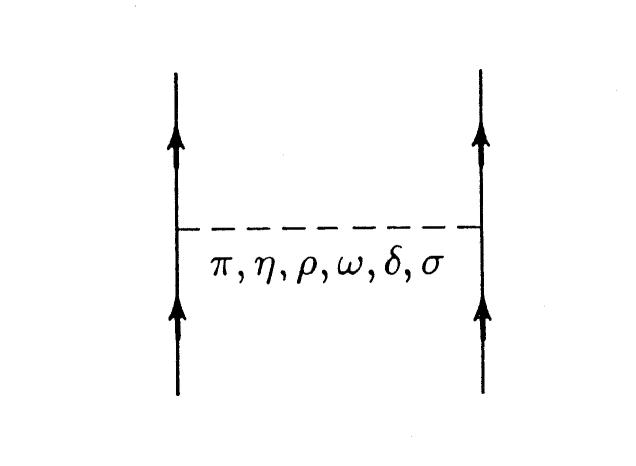
A typical one-boson-exchange model includes, about half a dozen of bosons with masses up to about 1 GeV, Fig. 1. Not all mesons are equally important. The leading actors are the following four particles:

• The pseudoscalar pion with a mass of about 138 MeV and isospin $I=1$ (isovector). It is the lightest meson and provides the long-range part of the potential and most of the tensor force.

• The isovector $\rho$ meson, a 2$\pi$ $P$-wave resonance of about 770 MeV. Its major effect is to cut down the tensor force provided by the pion at short range.

• The isoscalar $\omega$ meson, a 3$\pi$ resonance of 783 MeV and spin 1. It creates a strong repulsive central force of short range (‘repulsive core’) and the nuclear spin-orbit force.

• The scalar-isoscalar $f_{0}(500)$ or $\sigma$ boson with a mass around 500 MeV. It provides the crucial intermediate range attraction necessary for nuclear binding. The interpretation as a particle is controversial [26]. It may also be viewed as a simulation of effects of correlated $S$-wave 2$\pi$-exchange.

Obviously, just these four mesons can produce the major properties of the nuclear force.

Classic examples for OBE potentials (OBEPs) are the Bryan-Scott potentials started in the early 1960’s [28], but soon many other researchers got involved, too [29, 30]. Since it is suggestive to think of a potential as a function of $r$ (where $r$ denotes the distance between the centers of the two interacting nucleons), the OBEPs of the 1960’s where represented as local $r$-space potentials. Some groups continued to hold on to this tradition and, thus, the construction of improved $r$-space OBEPs continued well into the 1990’s [31].

An important advance during the 1970’s was the development of the relativistic OBEP [32, 33, 34]. In this model, the full, relativistic Feynman amplitudes for the various one-boson-exchanges are used to define the potential. These nonlocal expressions do not pose any numerical problems when used in momentum space and allow for a more quantitave descripton of $NN$ scattering. The the high-precision CD-Bonn potential [35] is of this nature.

2.2 Beyond the OBE approximation

Figure 2: The $2\pi$-exchange contribution to the $NN$ interaction as viewed by dispersion theory. Solid lines represent nucleons and dashed lines pions. Further explanations are given in the text.

Historically, one must understand that, after the failure of the pion theories in the 1950’s, the OBE model was considered a great success in the 1960’s [29].

On the other hand, one has to concede that the OBE model is a great simplification of the complicated scenario of a full meson theory for the $NN$ interaction. Therefore, in spite of the quantitative success of the OBEPs, one should be concerned about the approximations involved in the model. Major critical points include:

• The scalar isoscalar $\sigma$ ’meson’ of about 500 MeV.

• The neglect of all non-iterative diagrams.

• The role of meson-nucleon resonances.

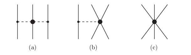
Two pions, when ’in the air’, can interact strongly. When in a relative $P$-wave $(L=1)$, they form a proper resonance, the $\rho$ meson. They can also interact in a relative $S$-wave $(L=0)$, which gives rise to the $\sigma$ boson. Whether the $\sigma$ is a proper resonance is controversial, even though the Particle Data Group lists an $f_{0}(500)$ or $\sigma(500)$ meson, but with a width 400-700 MeV [26]. What is for sure is that two pions have correlations, and if one doesn’t believe in the $\sigma$ as a two pion resonance, then one has to take these correlations into account. There are essentially two approaches that have been used to calculate these two-pion exchange contributions to the $NN$ interaction (which generates the intermediate range attraction): dispersion theory and field theory.

In the 1960’s, dispersion theory was developed out of frustration with the failure of a QFT for strong interactions in the 1950’s [16]. In the dispersion-theoretic approach the $NN$ amplitude is connected to the (empirical) $\pi N$ amplitude by causality (analyticity), unitarity, and crossing symmetry. Schematically this is shown in Fig. 2. The total diagram (a) is analysed in terms of two ’halves’ (b). The hatched ovals stand for all possible processes which a pion and a nucleon can undergo. This is made more explicit in (d) and (e). The hatched boxes represent baryon intermediate states including the nucleon. (Note that there are also crossed pion exchanges which are not shown.) The shaded circle stands for $\pi\pi$ scattering. Quantitatively, these processes are taken into account by using empirical information from $\pi N$ and $\pi\pi$ scattering (e. g. phase shifts) which represents the input for such a calculation. Dispersion relations then provide an on-shell $NN$ amplitude, which — with some kind of plausible prescription — is represented as a potential. The Stony Brook [36, 37] and Paris [38, 39] groups have pursued this approach. They could show that the intermediate-range part of the nuclear force is, indeed, decribed about right by the $2\pi$-exchange as obtained from dispersion integrals. To construct a complete potential, the $2\pi$-exchange contribution is complemented by one-pion and $\omega$ exchange. In addition to this, the Paris potential [40] contains a phenomenological short-range part for $r<1.5$ fm to improve the fit to the $NN$ data. For further details, we refer the interested reader to a pedagogical article by Vinh Mau [41].

Figure 3: Field-theoretic model for the $2\pi$-exchange. Notation as in Fig. 2. Double lines represent isobars. The hatched circles are $\pi\pi$ correlations. Further explanations are given in the text.

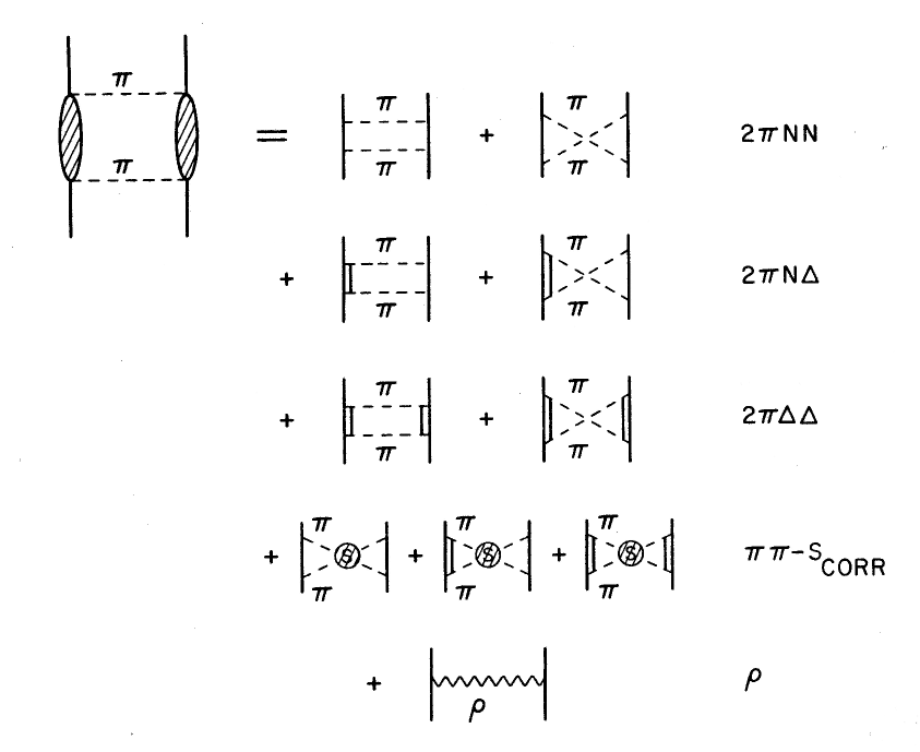
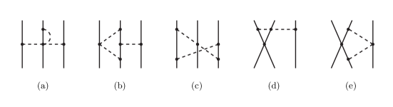
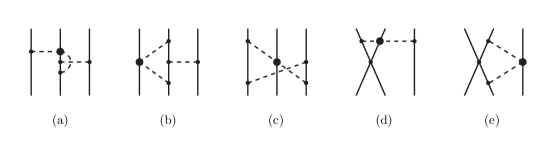
A first field-theoretic attempt towards the $2\pi$-exchange was undertaken by Lomon and Partovi [42]. Later, the more elaborated model shown in Fig. 3 was developed by the Bonn group [43]. The model includes contributions from isobars as well as from $\pi\pi$ correlations. This can be understood in analogy to the dispersion relations picture. In general, only the lowest $\pi N$ resonance, the so-called $\Delta$ isobar (spin 3/2, isospin 3/2, mass 1232 MeV), is taken into account. The contributions from other resonances have proven to be small for the low-energy $NN$ processes under consideration. A field-theoretic model treats the $\Delta$ isobar as an elementary (Rarita-Schwinger) particle. The six upper diagrams of Fig. 3 represent uncorrelated $2\pi$ exchange. The crossed (non-iterative) two-particle exchanges (second diagram in each row) are important. They guarantee the proper (very weak) isospin dependence due to characteristic cancelations in the isospin dependent parts of box and crossed box diagrams. Furthermore, their contribution is about as large as the one from the corresponding box diagrams (iterative diagrams); therefore, they are not negligible. In addition to the processes discussed, also correlated $2\pi$ exchange has to be included (lower two rows of Fig. 3). Quantitatively, these contributions are about as sizable as those from the uncorrelated processes. Graphs with virtual pairs are left out, because the pseudovector (gradient) coupling is used for the pion, in which case pair terms are small.

Figure 4: $\pi\rho$ contributions to the $NN$ interaction.

Besides the contributions from two pions, there are also contributions from the combination of other mesons. The combination of $\pi$ and $\rho$ is particularly significant, Fig. 4. This contribution is repulsive and important to suppress the 2$\pi$ exchange contribution at high momenta (or small distances), which is too strong by itself.

The Bonn Full Model [43], includes all the diagrams displayed in Figs. 3 and 4 plus single $\pi$ and $\omega$ exchange.

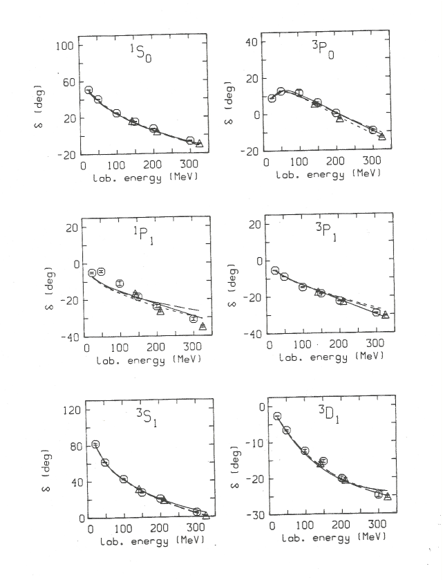
Having highly sophisticated models at hand, like the Paris and the Bonn potentials, allows to check the approximations made in the simple OBE model. As it turns out, the complicated 2$\pi$ exchange contributions to the $NN$ interaction tamed by the $\pi\rho$ diagrams can well be simulated by the single scalar isoscalar boson, the $\sigma$, with a mass around 550 MeV. In retrospect, this fact provides justification for the simple OBE model. To illustate this point, we show, in Figs. 5 and 6, the phase shift predictions from the Bonn [43] and Paris [40] potentials as well as a relativistic OBEP [27].

The most important result of Phase II is that meson exchange is an excellent phenomenology for describing nuclear forces. It allows for the construction of very quantitative models. Therefore, the high-precision $NN$ potentials constructed in the mid-1990’s are all based upon meson phenomenology [31, 35, 44]. However, with the rise of QCD to the ranks of the authoritative theory of strong interactions, meson-exchange is definitively just a model. This implies that if we ultimately wish to solve the nuclear force problem on the most fundamental grounds, then we have to begin all over again—starting with QCD.

Figure 5: Phase shifts of $np$ scattering from some “classic” meson-exchange models for the $NN$ interaction. Predictions are shown for the Bonn Full Model [43] (solid line), the Paris potential [40] (dashed), and a (relativistic) OBEP [27] (dotted). Phase parameters with total angular momentum $J\leq 1$ are displayed. Symbols represent results from $NN$ phase shift analyses.

Figure 6: Same as Fig. 5, but $J=2$ phase shifts and $J\leq 2$ mixing parameters are shown.

3 Phase III (1990 – 2020): Chiral Effective Field Theory

3.1 QCD and nuclear forces

Quantum chromodynamics provides the theoretical framework to describe strong interactions, namely interactions involving quarks and gluons. According to QCD, objects which carry color interact weakly at short distances and strongly at large distances, where the separation between the two regimes is about 1 fm. Naturally, short distances and long distances can be associated with high and low energies, respectively, causing the quarks to be confined into hadrons, which carry no color. At the same time, the weak nature of the force at high energies results into what is known as “asymptotic freedom”. (We note that these behaviors originate from the fact that QCD is a non-Abelian gauge field theory with color $SU(3)$ the underlying gauge group.) Therefore, QCD is perturbative at high energy, but strongly coupled at low-energy. The energies typical for nuclear physics are low and, thus, nucleons are appropriate degrees of freedom. The nuclear force can then be regarded as a residual color interaction acting between nucleons in a way similar to how the van der Waals forces bind neutral molecules. If described in terms of quark and gluon degrees of freedom, the interaction between nucleons is an extremely complex problem.

Therefore, during the first round of new attempts, QCD-inspired quark models [45] became popular. The positive aspect of these models is that they try to explain hadron structure and hadron-hadron interactions on an equal footing and, indeed, some of the gross features of the $NN$ interaction are explained successfully. However, on a critical note, it must be pointed out that these quark-based approaches are nothing but another set of models and, thus, do not represent fundamental progress. For the purpose of describing hadron-hadron interactions, one may equally well then stay with the simpler and much more quantitative meson models.

Alternatively, one may try to solve the problem with brute computing power by a method known as lattice QCD. In a recent paper [46], the nucleon-nucleon system is investigated at a pion mass of about 450 MeV. Over the range of energies that are studied, the scattering phase shifts in the ${}^{1}S_{0}$ and ${}^{3}S-D_{1}$ channels are found to be similar to those in nature and indicate a repulsive short-range component of the interaction. This result is then extrapolated to the physical pion mass with the help of chiral perturbation theory. The pion mass of 450 MeV is still too large to allow for reliable extrapolations, but the feasibility has been demonstrated and more progress can be expected for the near future. In a lattice calculation of a very different kind, the $NN$ potential was studied in Ref. [47]. The central component of this potential exhibits repulsion at the core as well as intermediate-range attraction. This is encouraging, but one must keep in mind that the pion masses employed in this study are still quite large. In summary, although calculations within lattice QCD are being performed and improved, they are computationally very costly, and thus they are useful, in practice, only to explore a few cases. Clearly, a different approach is necessary to address a full variety of nuclear structure problems.

3.2 An EFT for low-energy QCD

Around 1980/1990, a major breakthrough occurred when the nobel laureate Steven Weinberg applied the concept of an effective field theory (EFT) to low-energy QCD [48, 49, 50, 51, 52]. He simply wrote down the most general Lagrangian that is consistent with all the properties of low-energy QCD, since that would make this theory equivalent to low-energy QCD. A particularly important property is the so-called chiral symmetry, which is “spontaneously” broken. The effective degrees of freedom are then pions (the Goldstone bosons of the broken symmetry) and nucleons rather than quarks and gluons; heavy mesons and nucleon resonances are “integrated out”. So, the circle of history is closing and we are back to a pion theory (cf. Phase I) except that we have finally learned how to deal with it: broken chiral symmetry is a crucial constraint that generates and controls the dynamics and establishes a clear connection with the underlying theory, QCD. The constraint of chiral symmetry dictates that the pion couples to the nucleon via a derivative coupling ($\gamma_{5}\gamma^{\mu}\partial_{\mu}$). Recall that this coupling was already considered in the 1950’s [14], but discarded because it is not renormalizable. In the context of a fundamental quantum field theory, this coupling is, indeed, not renormalizable. However, the scenario is now different [53, 54]. The gradient coupling is revived in the context of an effective field theory. Such a theory, is organized order by order and, therefore, renormalized order by order. In each order, only a finite number of counter terms is needed to renormalize. Moreover, the calculation is carried out only up to a finite order at which the desired accuracy is achieved. Thus, everything is manageable.

For the order by order expansion of the EFT, an appropriate “large scale” needs to be identified. The large difference between the masses of the pions and the masses of the vector mesons, like $\rho(770)$ and $\omega(782)$, provides a clue. From that observation, one is prompted to take the pion mass as the identifier of the soft scale, $Q\sim m_{\pi}$, while the rho mass sets the hard scale, $\Lambda_{\chi}\sim m_{\rho}$, often referred to as the chiral-symmetry breaking scale. It is then natural to consider an expansion in terms of $Q/\Lambda_{\chi}$.

To summarize, an EFT program for nuclear forces involves the following steps:

1. Identify the low- and high-energy scales, and the degrees of freedom suitable for (low-energy) nuclear physics.

2. Recognize the symmetries of low-energy QCD and explore the mechanisms responsible of their breakings.

3. Build the most general Lagrangian which respects those (broken) symmetries.

4. Formulate a scheme to organize contributions in order of their importance. Clearly, this amounts to performing an expansion in terms of (low) momenta.

5. Using the expansion mentioned above, evaluate Feynman diagrams to the desired accuracy.

In what follows, we will discuss each of the steps above. Note that the first one has already been addressed, so we will move directly to the second one.

3.3 Symmetries of low-energy QCD

Our purpose here is to provide a compact introduction into (low-energy) QCD, with particular attention to the symmetries and their breakings. For more details the reader is referred to Refs. [55, 56].

3.3.1 Chiral symmetry

We begin with the QCD Lagrangian,

$${\cal L}_{\rm QCD}=\bar{q}(i\gamma^{\mu}{\cal D}_{\mu}-{\cal M})q-\frac{1}{4}{\cal G}_{\mu\nu,a}{\cal G}^{\mu\nu}_{a}$$ (1)

with the gauge-covariant derivative

$${\cal D}_{\mu}=\partial_{\mu}-ig\frac{\lambda_{a}}{2}{\cal A}_{\mu,a}$$ (2)

and the gluon field strength tensor

$${\cal G}_{\mu\nu,a}=\partial_{\mu}{\cal A}_{\nu,a}-\partial_{\nu}{\cal A}_{\mu,a}+gf_{abc}{\cal A}_{\mu,b}{\cal A}_{\nu,c}\,.$$ (3)

In the above, $q$ denotes the quark fields and ${\cal M}$ the quark mass matrix. Further, $g$ is the strong coupling constant and ${\cal A}_{\mu,a}$ are the gluon fields. Moreover, $\lambda_{a}$ are the Gell-Mann matrices and $f_{abc}$ the structure constants of the $SU(3)_{\rm color}$ Lie algebra $(a,b,c=1,\dots,8)$; summation over repeated indices is always implied. The gluon-gluon term in the last equation arises from the non-Abelian nature of the gauge theory and is the reason for the peculiar features of the color force.

The current masses of the up $(u)$, down $(d)$, and strange (s) quarks are in a $\overline{MS}$ scheme at a scale of $\mu\approx 2$ GeV [26]:

$$m_{u} = 2.3\pm 0.7\mbox{ MeV},$$ (4)

$$m_{d} = 4.8\pm 0.5\mbox{ MeV},$$ (5)

$$m_{s} = 95\pm 5\mbox{ MeV}.$$ (6)

These masses are small as compared to a typical hadronic scale such as the mass of a light hadron other than a Goldstone bosons, e.g., $m_{\rho}=0.78\mbox{ GeV}\approx 1\mbox{ GeV}$.

Thus it is relevant to discuss the QCD Lagrangian in the case when the quark masses vanish:

$${\cal L}_{\rm QCD}^{0}=\bar{q}i\gamma^{\mu}{\cal D}_{\mu}q-\frac{1}{4}{\cal G}_{\mu\nu,a}{\cal G}^{\mu\nu}_{a}\,.$$ (7)

Right- and left-handed quark fields are defined as

$$q_{R}=P_{R}q\,,\;\;\;q_{L}=P_{L}q\,,$$ (8)

with

$$P_{R}=\frac{1}{2}(1+\gamma_{5})\,,\;\;\;P_{L}=\frac{1}{2}(1-\gamma_{5})\,.$$ (9)

Then the Lagrangian can be rewritten as

$${\cal L}_{\rm QCD}^{0}=\bar{q}_{R}i\gamma^{\mu}{\cal D}_{\mu}q_{R}+\bar{q}_{L}i\gamma^{\mu}{\cal D}_{\mu}q_{L}-\frac{1}{4}{\cal G}_{\mu\nu,a}{\cal G}^{\mu\nu}_{a}\,.$$ (10)

This equation revels that the right- and left-handed components of massless quarks do not mix in the QCD Lagrangian. For the two-flavor case, this is $SU(2)_{R}\times SU(2)_{L}$ symmetry, also known as chiral symmetry. However, this symmetry is broken in two ways: explicitly and spontaneously.

3.3.2 Explicit symmetry breaking

The mass term $-\bar{q}{\cal M}q$ in the QCD Lagrangian Eq. (1) breaks chiral symmetry explicitly. To better see this, let’s rewrite ${\cal M}$ for the two-flavor case,

$${\cal M} = \left(\begin{array}[]{cc}m_{u}&0\\ 0&m_{d}\end{array}\right)$$ (13)

$$= \frac{1}{2}(m_{u}+m_{d})\left(\begin{array}[]{cc}1&0\\ 0&1\end{array}\right)+\frac{1}{2}(m_{u}-m_{d})\left(\begin{array}[]{cc}1&0\\ 0&-1\end{array}\right)$$ (18)

$$= \frac{1}{2}(m_{u}+m_{d})\;I+\frac{1}{2}(m_{u}-m_{d})\;\tau_{3}\,.$$ (19)

The first term in the last equation in invariant under $SU(2)_{V}$ (isospin symmetry) and the second term vanishes for $m_{u}=m_{d}$. Therefore, isospin is an exact symmetry if $m_{u}=m_{d}$. However, both terms in Eq. (19) break chiral symmetry. Since the up and down quark masses [Eqs. (4) and (5)] are small as compared to the typical hadronic mass scale of $\sim 1$ GeV, the explicit chiral symmetry breaking due to non-vanishing quark masses is very small.

3.3.3 Spontaneous symmetry breaking

A (continuous) symmetry is said to be spontaneously broken if a symmetry of the Lagrangian is not realized in the ground state of the system. There is evidence that the (approximate) chiral symmetry of the QCD Lagrangian is spontaneously broken—for dynamical reasons of nonperturbative origin which are not fully understood at this time. The most plausible evidence comes from the hadron spectrum.

From chiral symmetry, one naively expects the existence of degenerate hadron multiplets of opposite parity, i.e., for any hadron of positive parity one would expect a degenerate hadron state of negative parity and vice versa. However, these “parity doublets” are not observed in nature. For example, take the $\rho$-meson which is a vector meson of negative parity ($J^{P}=1^{-}$) and mass 776 MeV. There does exist a $1^{+}$ meson, the $a_{1}$, but it has a mass of 1230 MeV and, therefore, cannot be perceived as degenerate with the $\rho$. On the other hand, the $\rho$ meson comes in three charge states (equivalent to three isospin states), the $\rho^{\pm}$ and the $\rho^{0}$, with masses that differ by at most a few MeV. Thus, in the hadron spectrum, $SU(2)_{V}$ (isospin) symmetry is well observed, while axial symmetry is broken: $SU(2)_{R}\times SU(2)_{L}$ is broken down to $SU(2)_{V}$.

A spontaneously broken global symmetry implies the existence of (massless) Goldstone bosons. The Goldstone bosons are identified with the isospin triplet of the (pseudoscalar) pions, which explains why pions are so light. The pion masses are not exactly zero because the up and down quark masses are not exactly zero either (explicit symmetry breaking). Thus, pions are a truly remarkable species: they reflect spontaneous as well as explicit symmetry breaking. Goldstone bosons interact weakly at low energy. They are degenerate with the vacuum and, therefore, interactions between them must vanish at zero momentum and in the chiral limit ($m_{\pi}\rightarrow 0$).

3.4 Chiral effective Lagrangians

The next step in our EFT program is to build the most general Lagrangian consistent with the (broken) symmetries discussed above. An elegant formalism for the construction of such Lagrangians was developed by Callan, Coleman, Wess, and Zumino (CCWZ) [57] who developed the foundations of non-linear realizations of chiral symmetry from the point of view of group theory. The Lagrangians we give below are built upon the CCWZ formalism.

We already addressed the fact that the appropriate degrees of freedom are pions (Goldstone bosons) and nucleons. Because pion interactions must vanish at zero momentum transfer and in the limit of $m_{\pi}\rightarrow 0$, namely the chiral limit, the Lagrangian is expanded in powers of derivatives and pion masses. More precisely, the Lagrangian is expanded in powers of $Q/\Lambda_{\chi}$ where $Q$ stands for a (small) momentum or pion mass and $\Lambda_{\chi}\approx 1$ GeV is identified with the hard scale. These are the basic steps behind the chiral perturbative expansion.

Schematically, we can write the effective Lagrangian as

$${\cal L}={\cal L}_{\pi\pi}+{\cal L}_{\pi N}+{\cal L}_{NN}+\,\ldots\,,$$ (20)

where ${\cal L}_{\pi\pi}$ deals with the dynamics among pions, ${\cal L}_{\pi N}$ describes the interaction between pions and a nucleon, and ${\cal L}_{NN}$ contains two-nucleon contact interactions which consist of four nucleon-fields (four nucleon legs) and no meson fields. The ellipsis stands for terms that involve two nucleons plus pions and three or more nucleons with or without pions, relevant for nuclear many-body forces (an example for this in lowest order are the last two terms of Eq. (26), below). The individual Lagrangians are organized order by order:

$${\cal L}_{\pi\pi}={\cal L}_{\pi\pi}^{(2)}+{\cal L}_{\pi\pi}^{(4)}+\ldots\,,$$ (21)

$${\cal L}_{\pi N}={\cal L}_{\pi N}^{(1)}+{\cal L}_{\pi N}^{(2)}+{\cal L}_{\pi N}^{(3)}+{\cal L}_{\pi N}^{(4)}+{\cal L}_{\pi N}^{(5)}+\ldots,$$ (22)

and

$${\cal L}_{NN}={\cal L}^{(0)}_{NN}+{\cal L}^{(2)}_{NN}+{\cal L}^{(4)}_{NN}+{\cal L}^{(6)}_{NN}+\ldots\,,$$ (23)

where the superscript refers to the number of derivatives or pion mass insertions (chiral dimension) and the ellipsis stands for terms of higher dimensions.

Above, we have organized the Lagrangians by the number of derivatives or pion-masses. This is the standard way, appropriate particularly for considerations of $\pi$-$\pi$ and $\pi$-$N$ scattering. As it turns out (cf. Section 3.5.1), for interactions among nucleons, sometimes one makes use of the so-called index of the interaction,

$$\Delta\equiv d+\frac{n}{2}-2\,,$$ (24)

where $d$ is the number of derivatives or pion-mass insertions and $n$ the number of nucleon field operators (nucleon legs). We will now write down the Lagrangian in terms of increasing values of the parameter $\Delta$ and we will do so using the so-called heavy-baryon formalism which we indicate by a “hat” [58].

The leading-order Lagrangian reads,

$$\widehat{\cal L}^{\Delta=0} = \frac{1}{2}\partial_{\mu}\mbox{\boldmath{$\pi$}}\cdot\partial^{\mu}\mbox{\boldmath{$\pi$}}-\frac{1}{2}m_{\pi}^{2}\mbox{\boldmath{$\pi$}}^{2}$$ (25)

$$+\frac{1-4\alpha}{2f_{\pi}^{2}}(\mbox{\boldmath{$\pi$}}\cdot\partial_{\mu}\mbox{\boldmath{$\pi$}})(\mbox{\boldmath{$\pi$}}\cdot\partial^{\mu}\mbox{\boldmath{$\pi$}})-\frac{\alpha}{f_{\pi}^{2}}\mbox{\boldmath{$\pi$}}^{2}\partial_{\mu}\mbox{\boldmath{$\pi$}}\cdot\partial^{\mu}\mbox{\boldmath{$\pi$}}+\;\frac{8\alpha-1}{8f_{\pi}^{2}}m_{\pi}^{2}\mbox{\boldmath{$\pi$}}^{4}$$

$$+\bar{N}\left[i\partial_{0}-\frac{g_{A}}{2f_{\pi}}\;\mbox{\boldmath$\tau$}\cdot(\vec{\sigma}\cdot\vec{\nabla})\mbox{\boldmath$\pi$}-\frac{1}{4f_{\pi}^{2}}\;\mbox{\boldmath$\tau$}\cdot(\mbox{\boldmath$\pi$}\times\partial_{0}\mbox{\boldmath$\pi$})\right]N$$

$$+\bar{N}\left\{\frac{g_{A}(4\alpha-1)}{4f_{\pi}^{3}}\;(\mbox{\boldmath$\tau$}\cdot\mbox{\boldmath$\pi$})\left[\mbox{\boldmath$\pi$}\cdot(\vec{\sigma}\cdot\vec{\nabla})\mbox{\boldmath$\pi$}\right]\right.$$

$$\left.+\;\frac{g_{A}\alpha}{2f_{\pi}^{3}}\;\mbox{\boldmath$\pi$}^{2}\left[\mbox{\boldmath$\tau$}\cdot(\vec{\sigma}\cdot\vec{\nabla})\mbox{\boldmath$\pi$}\right]\right\}N$$

$$-\frac{1}{2}C_{S}\bar{N}N\bar{N}N-\frac{1}{2}C_{T}(\bar{N}\vec{\sigma}N)\cdot(\bar{N}\vec{\sigma}N)\;+\;\ldots\,,$$

and subleading Lagrangians are,

$$\widehat{\cal L}^{\Delta=1} = \bar{N}\left\{\frac{{\vec{\nabla}}^{2}}{2M_{N}}-\frac{ig_{A}}{4M_{N}f_{\pi}}\mbox{\boldmath$\tau$}\cdot\left[\vec{\sigma}\cdot\left(\stackrel{{\scriptstyle\leftarrow}}{{\nabla}}\partial_{0}\mbox{\boldmath$\pi$}-\partial_{0}\mbox{\boldmath$\pi$}\stackrel{{\scriptstyle\rightarrow}}{{\nabla}}\right)\right]\right.$$ (26)

$$\left.-\frac{i}{8M_{N}f_{\pi}^{2}}\mbox{\boldmath$\tau$}\cdot\left[\stackrel{{\scriptstyle\leftarrow}}{{\nabla}}\cdot(\mbox{\boldmath$\pi$}\times\vec{\nabla}\mbox{\boldmath$\pi$})-(\mbox{\boldmath$\pi$}\times\vec{\nabla}\mbox{\boldmath$\pi$})\cdot\stackrel{{\scriptstyle\rightarrow}}{{\nabla}}\right]\right\}N$$

$$+\bar{N}\left[4c_{1}m_{\pi}^{2}-\frac{2c_{1}}{f_{\pi}^{2}}\,m_{\pi}^{2}\,\mbox{\boldmath$\pi$}^{2}\,+\,\left(c_{2}-\frac{g_{A}^{2}}{8M_{N}}\right)\frac{1}{f_{\pi}^{2}}(\partial_{0}\mbox{\boldmath{$\pi$}}\cdot\partial_{0}\mbox{\boldmath{$\pi$}})\right.$$

$$\left.+\,\frac{c_{3}}{f_{\pi}^{2}}\,(\partial_{\mu}\mbox{\boldmath{$\pi$}}\cdot\partial^{\mu}\mbox{\boldmath{$\pi$}})-\,\left(c_{4}+\frac{1}{4M_{N}}\right)\frac{1}{2f_{\pi}^{2}}\epsilon^{ijk}\epsilon^{abc}\sigma^{i}\tau^{a}(\partial^{j}\pi^{b})(\partial^{k}\pi^{c})\right]N$$

$$-\frac{D}{4f_{\pi}}(\bar{N}N)\bar{N}\left[\mbox{\boldmath$\tau$}\cdot(\vec{\sigma}\cdot\vec{\nabla})\mbox{\boldmath$\pi$}\right]N$$

$$-\frac{1}{2}E(\bar{N}N)(\bar{N}\mbox{\boldmath$\tau$}N)\cdot(\bar{N}\mbox{\boldmath$\tau$}N)\;+\;\ldots\,,$$

$$\widehat{\cal L}^{\Delta=2} = \;{\cal L}^{(4)}_{\pi\pi}\;+\;\widehat{\cal L}^{(3)}_{\pi N}\;+\;\widehat{\cal L}^{(2)}_{NN}\;+\;\ldots\,,$$ (27)

$$\widehat{\cal L}^{\Delta=3} = \;\widehat{\cal L}^{(4)}_{\pi N}\;+\;\ldots\,,$$ (28)

$$\widehat{\cal L}^{\Delta=4} = \;\widehat{\cal L}^{(5)}_{\pi N}\;+\;\widehat{\cal L}^{(4)}_{NN}\;+\;\ldots\,.$$ (29)

$$\widehat{\cal L}^{\Delta=6} = \;\widehat{\cal L}^{(6)}_{NN}\;+\;\ldots\,,$$ (30)

where we included terms relevant for a calculation of the two-nucleon force up to sixth order. The Lagrangians $\widehat{\cal L}^{(3)}_{\pi N}$ and $\widehat{\cal L}^{(4)}_{\pi N}$ can be found in Ref. [59]. The pion fields are denoted by $\bm{\pi}$ and the heavy baryon nucleon field by $N$ ($\bar{N}=N^{\dagger}$). Furthermore, $g_{A}$, $f_{\pi}$, $m_{\pi}$, and $M_{N}$ are the axial-vector coupling constant, pion decay constant, pion mass, and nucleon mass, respectively. The $c_{i}$ are low-energy constants (LECs) from the dimension two $\pi N$ Lagrangian and $\alpha$ is a parameter that appears in the expansion of a $SU(2)$ matrix $U$ in powers of the pion fields, see Ref. [55] for more details. Results are independent of $\alpha$.

The lowest order (or leading order) $NN$ Lagrangian has no derivatives and reads [52]

$$\widehat{\cal L}^{(0)}_{NN}=-\frac{1}{2}C_{S}\bar{N}N\bar{N}N-\frac{1}{2}C_{T}(\bar{N}\vec{\sigma}N)\cdot(\bar{N}\vec{\sigma}N)\,,$$ (31)

where $C_{S}$ and $C_{T}$ are free paramters to be determined by fitting to the $NN$ data.

The second order $NN$ Lagrangian, $\widehat{\cal L}^{(2)}_{NN}$, can be found in Ref. [60]. The $NN$ contact potentials derived from some of the $NN$ Lagrangians are given in Sec. 3.6.1.

3.5 Nuclear forces from EFT: Overview

We proceed here with discussing the various steps towards a derivation of nuclear forces from EFT. In this section, we will discuss the expansion we are using in more details as well as the various Feynman diagrams as they emerge at each order.

3.5.1 Chiral perturbation theory and power counting

An infinite number of Feynman diagrams can be evaluated from the effective Langrangians and so one needs to be able to organize these diagrams in order of their importance. Chiral perturbation theory (ChPT) provides such organizational scheme.

In ChPT, graphs are analyzed in terms of powers of small external momenta over the large scale: $(Q/\Lambda_{\chi})^{\nu}$, where $Q$ is generic for a momentum (nucleon three-momentum or pion four-momentum) or a pion mass and $\Lambda_{\chi}\sim 1$ GeV is the chiral symmetry breaking scale (hadronic scale, hard scale). Determining the power $\nu$ has become known as power counting.

For the moment, we will consider only so-called irreducible graphs. By definition, an irreducible graph is a diagram that cannot be separated into two by cutting only nucleon lines. Following the Feynman rules of covariant perturbation theory, a nucleon propagator carries the dimension $Q^{-1}$, a pion propagator $Q^{-2}$, each derivative in any interaction is $Q$, and each four-momentum integration $Q^{4}$. This is also known as naive dimensional analysis. Applying then some topological identities, one obtains for the power of an irreducible diagram involving $A$ nucleons [55]

$$\nu=-2+2A-2C+2L+\sum_{i}\Delta_{i}\,,$$ (32)

with

$$\Delta_{i}\equiv d_{i}+\frac{n_{i}}{2}-2\,.$$ (33)

In the two equations above: for each vertex $i$, $C$ represents the number of individually connected parts of the diagram while $L$ is the number of loops; $d_{i}$ indicates how many derivatives or pion masses are present and $n_{i}$ the number of nucleon fields. The summation extends over all vertices present in that particular diagram. Notice also that chiral symmetry implies $\Delta_{i}\geq 0$. Interactions among pions have at least two derivatives ($d_{i}\geq 2,n_{i}=0$), while interactions between pions and a nucleon have one or more derivatives ($d_{i}\geq 1,n_{i}=2$). Finally, pure contact interactions among nucleons ($n_{i}=4$) have $d_{i}\geq 0$. In this way, a low-momentum expansion based on chiral symmetry can be constructed.

Naturally, the powers must be bounded from below for the expansion to converge. This is in fact the case, with $\nu\geq 0$.

Furthermore, the power formula Eq. (32) allows to predict the leading orders of connected multi-nucleon forces. Consider a $m$-nucleon irreducibly connected diagram ($m$-nucleon force) in an $A$-nucleon system ($m\leq A$). The number of separately connected pieces is $C=A-m+1$. Inserting this into Eq. (32) together with $L=0$ and $\sum_{i}\Delta_{i}=0$ yields $\nu=2m-4$. Thus, two-nucleon forces ($m=2$) appear at $\nu=0$, three-nucleon forces ($m=3$) at $\nu=2$ (but they happen to cancel at that order), and four-nucleon forces at $\nu=4$ (they don’t cancel). More about this in the next sub-section.

For later purposes, we note that for an irreducible $NN$ diagram ($A=2$, $C=1$), the power formula collapses to the very simple expression

$$\nu=2L+\sum_{i}\Delta_{i}\,.$$ (34)

To summarize, at each order $\nu$ we only have a well defined number of diagrams, which renders the theory feasible from a practical standpoint. The magnitude of what has been left out at order $\nu$ can be estimated (in a very simple way) from $(Q/\Lambda_{\chi})^{\nu+1}$. The ability to calculate observables (in principle) to any degree of accuracy gives the theory its predictive power.

3.5.2 The ranking of nuclear forces

Figure 7: Hierarchy of nuclear forces in ChPT. Solid lines represent nucleons and dashed lines pions. Small dots, large solid dots, solid squares, triangles, diamonds, and stars denote vertices of index $\Delta_{i}=\,$ 0, 1, 2, 3, 4, and 6, respectively. Further explanations are given in the text.

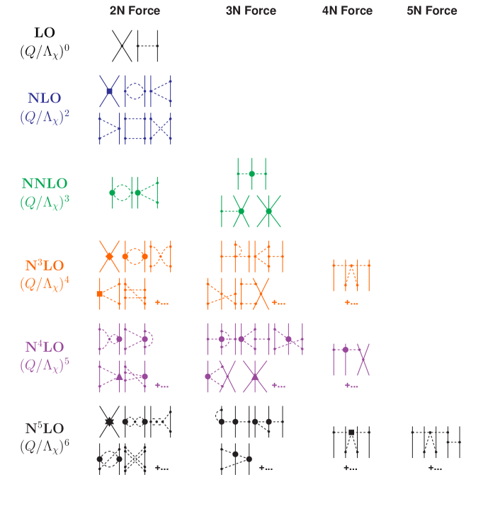
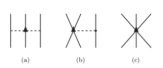
As shown in Fig. 7, nuclear forces appear in ranked orders in accordance with the power counting scheme.

The lowest power is $\nu=0$, also known as the leading order (LO). At LO we have only two contact contributions with no momentum dependence ($\sim Q^{0}$). They are signified by the four-nucleon-leg diagram with a small-dot vertex shown in the first row of Fig. 7. Besides this, we have the static one-pion exchange (1PE), also shown in the first row of Fig. 7.

In spite of its simplicity, this rough description contains some of the main attributes of the $NN$ force. First, through the 1PE it generates the tensor component of the force known to be crucial for the two-nucleon bound state. Second, it predicts correctly $NN$ phase parameters for high partial waves. At LO, the two terms which result from a partial-wave expansion of the contact term impact states of zero orbital angular momentum and produce attraction at short- and intermediate-range.

Notice that there are no terms with power $\nu=1$, as they would violate parity conservation and time-reversal invariance.

The next order is then $\nu=2$, next-to-leading order, or NLO.

Note that the two-pion exchange (2PE) makes its first appearance at this order, and thus it is referred to as the “leading 2PE”. As is well known from decades of nuclear physics, this contribution is essential for a realistic account of the intermediate-range attraction. However, the leading 2PE has insufficient strength, for the following reason: the loops present in the diagrams which involve pions carry the power $\nu=2$ [cf. Eq. (34)], and so only $\pi NN$ and $\pi\pi NN$ vertices with $\Delta_{i}=0$ are allowed at this order. These vertices are known to be weak. Moreover, seven new contacts appear at this order which impact $L=0$ and $L=1$ states. (As always, two-nucleon contact terms are indicated by four-nucleon-leg diagrams and a vertex of appropriate shape, in this case a solid square.) At this power, the appropriate operators include spin-orbit, central, spin-spin, and tensor terms, namely all the spin and isospin operator structures needed for a realistic description of the 2NF, although the medium-range attraction still lacks sufficient strength.

At the next order, $\nu=3$ or next-to-next-to-leading order (NNLO), the 2PE contains the so-called $\pi\pi NN$ seagull vertices with two derivatives. These vertices (proportional to the $c_{i}$ LECs, Eq. (26), and denoted by a large solid dot in Fig. 7), simulate correlated 2PE and intermediate $\Delta(1232)$-isobar contributions. Consistent with what the meson theory of the nuclear forces [40, 43] (cf. Sec. 2) has shown since a long time concerning the importance of these effects, at this order the 2PE finally provides medium-range attraction of realistic strength, bringing the description of the $NN$ force to an almost quantitative level. No new contacts become available at NNLO.

The discussion above reveals how two- and many-nucleon forces are generated and increase in number as we move to higher orders. Three-nucleon forces appear at NLO, but their net contribution vanishes at this order [61]. The first non-zero 3NF contribution is found at NNLO [62, 63]. It is therefore easy to understand why 3NF are very weak as compared to the 2NF which contributes already at $(Q/\Lambda_{\chi})^{0}$.

For $\nu=4$, or next-to-next-to-next-to-leading order (N³LO), we display some representative diagrams in Fig. 7. There is a large attractive one-loop 2PE contribution (the bubble diagram with two large solid dots $\sim c_{i}^{2}$), which slightly over-estimates the 2NF attraction at medium range. Two-pion-exchange graphs with two loops are seen at this order, together with three-pion exchange (3PE), which was determined to be very weak at N³LO [64, 65]. The most important feature at this order is the presence of 15 additional contacts $\sim Q^{4}$, signified by the four-nucleon-leg diagram in the figure with the diamond-shaped vertex. These contacts impact states with orbital angular momentum up to $L=2$, and are the reason for the quantitative description of the two-nucleon force (up to approximately 300 MeV in terms of laboratory energy) at this order [55, 66]. More 3NF diagrams show up at N³LO, as well as the first contributions to four-nucleon forces (4NF). We then see that forces involving more and more nucleons appear for the first time at higher and higher orders, which gives theoretical support to the fact that 2NF $\gg$ 3NF $\gg$ 4NF ….

Further 2PE and 3PE occur at N⁴LO (fifth order). The contribution to the 2NF at this order has been first calculated by Entem et al. [67]. It turns out to be moderately repulsive, thus compensating for the attractive surplus generated at N³LO by the bubble diagram with two solid dots. The long- and intermediate-range 3NF contributions at this order have been evaluated [59, 68], but not yet applied in nuclear structure calculations. They are expected to be sizeable. Moreover, a new set of 3NF contact terms appears [69]. The N⁴LO 4NF has not been derived yet. Due to the subleading $\pi\pi NN$ seagull vertex (large solid dot $\sim c_{i}$), this 4NF could be sizeable.

Finally turning to N⁵LO (sixth order): The dominant 2PE and 3PE contributions to the 2NF have been derived by Entem et al. in Ref. [70], which represents the most sophisticated investigation ever conducted in chiral EFT for the $NN$ system. The effects are small indicating the desired trend towards convergence of the chiral expansion for the 2NF. Moreover, a new set of 26 $NN$ contact terms $\sim Q^{6}$ occurs that contributes up to $F$-waves (represented by the $NN$ diagram with a star in Fig. 7) bringing the total number of $NN$ contacts to 50 [71]. The three-, four-, and five-nucleon forces of this order have not yet been derived.

Figure 8: Phase-shifts of neutron-proton scattering in $G$ waves at all orders of ChPT from LO to N⁵LO. The filled and open circles represent the results from the Nijmegen multi-energy $np$ phase-shift analysis [72] and the GWU single-energy $np$ analysis SP07 [73], respectively.

To summarize, we show in Fig. 8 the contributions to the phase shifts of peripheral $NN$ scattering through all orders from LO to N⁵LO as obtained from a perturbative calculation. Note that the difference between the LO prediction (one-pion-exchange, dotted line) and the data (filled and open circles) is to be provided by two- and three-pion exchanges, i.e. the intermediate-range part of the nuclear force. How well that is accomplished is a crucial test for any theory of nuclear forces. NLO produces only a small contribution, but N²LO creates substantial intermediate-range attraction (most clearly seen in ${}^{1}G_{4}$, ${}^{3}G_{5}$). In fact, N²LO is the largest contribution among all orders. This is due to the one-loop $2\pi$-exchange triangle diagram which involves one $\pi\pi NN$-contact vertex proportional to $c_{i}$. As discussed, the one-loop $2\pi$-exchange at N²LO is attractive and describes the intermediate-range attraction of the nuclear force about right. At N³LO, more one-loop 2PE is added by the bubble diagram with two $c_{i}$-vertices, a contribution that seemingly is overestimating the attraction. This attractive surplus is then compensated by the prevailingly repulsive two-loop $2\pi$- and $3\pi$-exchanges that occur at N⁴LO and N⁵LO.

In this context, it is worth noting that also in conventional meson theory [43] (Sec. 2.2) the one-loop models for the 2PE contribution always show some excess of attraction (cf. Fig. 10 of Ref. [55]). The same is true for the dispersion theoretic approach pursued by the Paris group (see, e. g., the predictions for ${}^{1}D_{2}$, ${}^{3}D_{2}$, and ${}^{3}D_{3}$ in Fig. 8 of Ref. [41] which are all too attractive). In conventional meson theory, this attraction is reduced by heavy-meson exchanges ($\rho$-, $\omega$-, and $\pi\rho$-exchange) which, however, has no place in chiral effective field theory (as a finite-range contribution). Instead, in the latter approach, two-loop $2\pi$- and $3\pi$-exchanges provide the corrective action.

3.6 Quantitative chiral $NN$ potentials

In the previous section, we mainly discussed the pion-exchange contributions to the $NN$ interaction. They describe the long- and intermediate-range parts of the nuclear force, which are governed by chiral symmetry and rule the peripheral partial waves (cf. Fig. 8). However, for a “complete” nuclear force, we have to describe correctly all partial waves, including the lower ones. In fact, in calculations of $NN$ observables at low energies (cross sections, analyzing powers, etc.), the partial waves with $L\leq 2$ are the most important ones, generating the largest contributions. The same is true for microscopic nuclear structure calculations. The lower partial waves are dominated by the dynamics at short distances. Therefore, we need to look now more closely into the short-range part of the $NN$ potential.

3.6.1 $NN$ contact terms

In conventional meson theory (Sec. 2), the short-range nuclear force is described by the exchange of heavy mesons, notably the $\omega(782)$. Qualitatively, the short-distance behavior of the $NN$ potential is obtained by Fourier transform of the propagator of a heavy meson,

$$\int d^{3}q\frac{e^{i{\vec{q}}\cdot{\vec{r}}}}{m^{2}_{\omega}+{\vec{q}}^{2}}\;\sim\;\frac{e^{-m_{\omega}r}}{r}\;.$$ (35)

ChPT is an expansion in small momenta $Q$, too small to resolve structures like a $\rho(770)$ or $\omega(782)$ meson, because $Q\ll\Lambda_{\chi}\approx m_{\rho,\omega}$. But the latter relation allows us to expand the propagator of a heavy meson into a power series,

$$\frac{1}{m^{2}_{\omega}+Q^{2}}\approx\frac{1}{m^{2}_{\omega}}\left(1-\frac{Q^{2}}{m^{2}_{\omega}}+\frac{Q^{4}}{m^{4}_{\omega}}-+\ldots\right),$$ (36)

where the $\omega$ is representative for any heavy meson of interest. The above expansion suggests that it should be possible to describe the short distance part of the nuclear force simply in terms of powers of $Q/m_{\omega}$, which fits in well with our over-all power expansion since $Q/m_{\omega}\approx Q/\Lambda_{\chi}$. Since such terms act directly between nucleons, they are dubbed contact terms.

Contact terms play an important role in renormalization. Regularization of the loop integrals that occur in multi-pion exchange diagrams typically generates polynomial terms with coefficients that are, in part, infinite or scale dependent (cf. Appendix B of Ref. [55]). Contact terms absorb infinities and remove scale dependences, which is why they are also known as counter terms.

Due to parity, only even powers of $Q$ are allowed. Thus, the expansion of the contact potential is formally given by

$$V_{\rm ct}=V_{\rm ct}^{(0)}+V_{\rm ct}^{(2)}+V_{\rm ct}^{(4)}+V_{\rm ct}^{(6)}+\ldots\;,$$ (37)

where the supersript denotes the power or order.

We will now present, one by one, the various orders of $NN$ contact terms.

Zeroth order (LO)

The contact Lagrangian $\widehat{\cal L}^{(0)}_{NN}$, Eq. (31), which is part of $\widehat{\cal L}^{\Delta=0}$, Eq. (25), leads to the following $NN$ contact potential,

$$V_{\rm ct}^{(0)}(\vec{p^{\prime}},\vec{p})=C_{S}+C_{T}\,\vec{\sigma}_{1}\cdot\vec{\sigma}_{2}\,,$$ (38)

and, in terms of partial waves, we have

$$V_{\rm ct}^{(0)}(^{1}S_{0}) = \widetilde{C}_{{}^{1}S_{0}}=4\pi\,(C_{S}-3\,C_{T})$$

$$V_{\rm ct}^{(0)}(^{3}S_{1}) = \widetilde{C}_{{}^{3}S_{1}}=4\pi\,(C_{S}+C_{T})\,.$$ (39)

Second order (NLO)

The contact Lagrangian $\widehat{\cal L}^{(2)}_{NN}$, which is part of $\widehat{\cal L}^{\Delta=2}$, Eq. (27), generates the following $NN$ contact potential

$$V_{\rm ct}^{(2)}(\vec{p^{\prime}},\vec{p}) = C_{1}\,q^{2}+C_{2}\,k^{2}$$ (40)

$$+ \left(C_{3}\,q^{2}+C_{4}\,k^{2}\right)\vec{\sigma}_{1}\cdot\vec{\sigma}_{2}$$

$$+ C_{5}\left(-i\vec{S}\cdot(\vec{q}\times\vec{k})\right)$$

$$+ C_{6}\,(\vec{\sigma}_{1}\cdot\vec{q})\,(\vec{\sigma}_{2}\cdot\vec{q})$$

$$+ C_{7}\,(\vec{\sigma}_{1}\cdot\vec{k})\,(\vec{\sigma}_{2}\cdot\vec{k})\,,$$

with partial-wave decomposition

$$V_{\rm ct}^{(2)}(^{1}S_{0}) = C_{{}^{1}S_{0}}(p^{2}+{p^{\prime}}^{2})$$

$$V_{\rm ct}^{(2)}(^{3}P_{0}) = C_{{}^{3}P_{0}}\,pp^{\prime}$$

$$V_{\rm ct}^{(2)}(^{1}P_{1}) = C_{{}^{1}P_{1}}\,pp^{\prime}$$

$$V_{\rm ct}^{(2)}(^{3}P_{1}) = C_{{}^{3}P_{1}}\,pp^{\prime}$$

$$V_{\rm ct}^{(2)}(^{3}S_{1}) = C_{{}^{3}S_{1}}(p^{2}+{p^{\prime}}^{2})$$

$$V_{\rm ct}^{(2)}(^{3}S_{1}-^{3}D_{1}) = C_{{}^{3}S_{1}-^{3}D_{1}}p^{2}$$

$$V_{\rm ct}^{(2)}(^{3}D_{1}-^{3}S_{1}) = C_{{}^{3}S_{1}-^{3}D_{1}}{p^{\prime}}^{2}$$

$$V_{\rm ct}^{(2)}(^{3}P_{2}) = C_{{}^{3}P_{2}}\,pp^{\prime}$$ (41)

which obviously contributes up to $P$ waves.

Fourth order (N³LO)

The contact potential of order four reads

$$V_{\rm ct}^{(4)}(\vec{p^{\prime}},\vec{p}) = D_{1}\,q^{4}+D_{2}\,k^{4}+D_{3}\,q^{2}k^{2}+D_{4}\,(\vec{q}\times\vec{k})^{2}$$ (42)

$$+ \left(D_{5}\,q^{4}+D_{6}\,k^{4}+D_{7}\,q^{2}k^{2}+D_{8}\,(\vec{q}\times\vec{k})^{2}\right)\vec{\sigma}_{1}\cdot\vec{\sigma}_{2}$$

$$+ \left(D_{9}\,q^{2}+D_{10}\,k^{2}\right)\left(-i\vec{S}\cdot(\vec{q}\times\vec{k})\right)$$

$$+ \left(D_{11}\,q^{2}+D_{12}\,k^{2}\right)(\vec{\sigma}_{1}\cdot\vec{q})\,(\vec{\sigma}_{2}\cdot\vec{q})$$

$$+ \left(D_{13}\,q^{2}+D_{14}\,k^{2}\right)(\vec{\sigma}_{1}\cdot\vec{k})\,(\vec{\sigma}_{2}\cdot\vec{k})$$

$$+ D_{15}\left(\vec{\sigma}_{1}\cdot(\vec{q}\times\vec{k})\,\,\vec{\sigma}_{2}\cdot(\vec{q}\times\vec{k})\right).$$

The rather lengthy partial-wave expressions of this order are given in Appendix E of Ref. [55]. These contacts affect partial waves up to $D$ waves.

Sixth order (N⁵LO)

At sixth order, 26 new contact terms appear, bringing the total number to 50. These terms as well as their partial-wave decomposition have been worked out in Ref. [71]. They contribute up to $F$-waves. So far, these terms have not been used in the construction of $NN$ potentials.

3.6.2 Definition of $NN$ potential

We have now rounded up everything needed for a realistic nuclear force—long, intermediate, and short ranged components—and so we can finally proceed to the lower partial waves. However, here we encounter another problem. The two-nucleon system at low angular momentum, particularly in $S$ waves, is characterized by the presence of a shallow bound state (the deuteron) and large scattering lengths. Thus, perturbation theory does not apply. In contrast to $\pi$-$\pi$ and $\pi$-$N$, the interaction between nucleons is not suppressed in the chiral limit ($Q\rightarrow 0$). Weinberg [52] showed that the strong enhancement of the scattering amplitude arises from purely nucleonic intermediate states (“infrared enhancement”). He therefore suggested to use perturbation theory to calculate the $NN$ potential (i.e., the irreducible graphs) and to apply this potential in a scattering equation to obtain the $NN$ amplitude. We will follow this prescription.

The potential $V$ as discussed in previous sections is, in principal, an invariant amplitude and, thus, satisfies a relativistic scattering equation, for which we choose the BbS equation [74], which reads explicitly,

$${T}({\vec{p}}~{}^{\prime},{\vec{p}})={V}({\vec{p}}~{}^{\prime},{\vec{p}})+\int\frac{d^{3}p^{\prime\prime}}{(2\pi)^{3}}\>{V}({\vec{p}}~{}^{\prime},{\vec{p}}~{}^{\prime\prime})\>\frac{M_{N}^{2}}{E_{p^{\prime\prime}}}\>\frac{1}{{p}^{2}-{p^{\prime\prime}}^{2}+i\epsilon}\>{T}({\vec{p}}~{}^{\prime\prime},{\vec{p}})$$ (43)

with $E_{p^{\prime\prime}}\equiv\sqrt{M_{N}^{2}+{p^{\prime\prime}}^{2}}$. The advantage of using a relativistic scattering equation is that it automatically includes relativistic corrections to all orders. Thus, in the scattering equation, no propagator modifications are necessary when raising the order to which the calculation is conducted.

Defining

$$\widehat{V}({\vec{p}}~{}^{\prime},{\vec{p}})\equiv\frac{1}{(2\pi)^{3}}\sqrt{\frac{M_{N}}{E_{p^{\prime}}}}\>{V}({\vec{p}}~{}^{\prime},{\vec{p}})\>\sqrt{\frac{M_{N}}{E_{p}}}$$ (44)

and

$$\widehat{T}({\vec{p}}~{}^{\prime},{\vec{p}})\equiv\frac{1}{(2\pi)^{3}}\sqrt{\frac{M_{N}}{E_{p^{\prime}}}}\>{T}({\vec{p}}~{}^{\prime},{\vec{p}})\>\sqrt{\frac{M_{N}}{E_{p}}}\,,$$ (45)

where the factor $1/(2\pi)^{3}$ is added for convenience, the BbS equation collapses into the usual, nonrelativistic Lippmann-Schwinger (LS) equation,

$$\widehat{T}({\vec{p}}~{}^{\prime},{\vec{p}})=\widehat{V}({\vec{p}}~{}^{\prime},{\vec{p}})+\int d^{3}p^{\prime\prime}\>\widehat{V}({\vec{p}}~{}^{\prime},{\vec{p}}~{}^{\prime\prime})\>\frac{M_{N}}{{p}^{2}-{p^{\prime\prime}}^{2}+i\epsilon}\>\widehat{T}({\vec{p}}~{}^{\prime\prime},{\vec{p}})\,.$$ (46)

Since $\widehat{V}$ satisfies Eq. (46), it can be used like a nonrelativistic potential, and $\widehat{T}$ may be perceived as the conventional nonrelativistic $T$-matrix.

3.6.3 Regularization and non-perturbative renormalization

Iteration of $\widehat{V}$ in the LS equation, Eq. (46), requires cutting $\widehat{V}$ off for high momenta to avoid infinities. This is consistent with the fact that ChPT is a low-momentum expansion which is valid only for momenta $Q\ll\Lambda_{\chi}\approx 1$ GeV. Therefore, the potential $\widehat{V}$ is multiplied with the regulator function $f(p^{\prime},p)$,

$${\widehat{V}}(\vec{p}~{}^{\prime},{\vec{p}})\longmapsto{\widehat{V}}(\vec{p}~{}^{\prime},{\vec{p}})\,f(p^{\prime},p)$$ (47)

with

$$f(p^{\prime},p)=\exp[-(p^{\prime}/\Lambda)^{2n}-(p/\Lambda)^{2n}]\,,$$ (48)

such that

$${\widehat{V}}(\vec{p}~{}^{\prime},{\vec{p}})\,f(p^{\prime},p)\approx{\widehat{V}}(\vec{p}~{}^{\prime},{\vec{p}})\left\{1-\left[\left(\frac{p^{\prime}}{\Lambda}\right)^{2n}+\left(\frac{p}{\Lambda}\right)^{2n}\right]+\ldots\right\}\,.$$ (49)

Typical choices for the cutoff parameter $\Lambda$ that appears in the regulator are $\Lambda\approx 0.5\mbox{ GeV}<\Lambda_{\chi}\approx 1$ GeV.

Equation (49) provides an indication of the fact that the exponential cutoff does not necessarily affect the given order at which the calculation is conducted. For sufficiently large $n$, the regulator introduces contributions that are beyond the given order. Assuming a good rate of convergence of the chiral expansion, such orders are small as compared to the given order and, thus, do not affect the accuracy at the given order. In calculations, one uses, of course, the exponential form, Eq. (48), and not the expansion Eq. (49).

It is pretty obvious that results for the $T$-matrix may depend sensitively on the regulator and its cutoff parameter. This is acceptable if one wishes to build models. For example, the meson models of the past [27, 43] (Sec. 2) always depended sensitively on the choices for the cutoff parameters, and they were welcome as additional fit parameters to further improve the reproduction of the $NN$ data. However, the EFT approach wishes to be more fundamental in nature and not just another model.

In field theories, divergent integrals are not uncommon and methods have been devised for how to deal with them. One regulates the integrals and then removes the dependence on the regularization parameters (scales, cutoffs) by renormalization. In the end, the theory and its predictions do not depend on cutoffs or renormalization scales.

Renormalizable quantum field theories, like QED, have essentially one set of prescriptions that takes care of renormalization through all orders. In contrast, EFTs are renormalized order by order, i. e., each order comes with the counter terms needed to renormalize that order. Note that this applies only to perturbative calculations. The $NN$ potential is calculated perturbatively and hence properly renormalized.

However, the story is different for the $NN$ amplitude ($T$-matrix) that results from a solution of the LS equation, Eq. (46), which is a nonperturbative resummation of the potential. This resummation is necessary in nuclear EFT because nuclear physics is characterized by bound states which are nonperturbative in nature. EFT power counting may be different for nonperturbative processes as compared to perturbative ones. Such difference may be caused by the infrared enhancement of the reducible diagrams generated in the LS equation.

Weinberg’s implicit assumption [51, 54] was that the counterterms introduced to renormalize the perturbatively calculated potential, based upon naive dimensional analysis (“Weinberg counting”), are also sufficient to renormalize the nonperturbative resummation of the potential in the LS equation. In 1996, Kaplan, Savage, and Wise (KSW) [75] pointed out that there are problems with the Weinberg scheme if the LS equation is renormalized by minimally-subtracted dimensional regularization. This criticism resulted in a flurry of publications on the renormalization of the nonperturbative $NN$ problem and I like to refer the interested reader to Ref. [55] for a comprehensive consideration of the issue.

3.6.4 $NN$ potentials order by order

Figure 9: Chiral expansion of neutron-proton scattering as represented by the phase shifts for $J\leq 1$. Five orders ranging from LO to N⁴LO are shown as denoted. Filled and open circles as in Fig. 8. (From Ref. [77].)

Figure 10: Same as Fig. 9, but for ${}^{3}P_{2}$, $D$-waves, and mixing parameters $\epsilon_{1}$ and $\epsilon_{2}$.

Table 1: $\chi^{2}/$datum for the fit of the 2016 $NN$ data base by $NN$ potentials at various orders of chiral EFT. (From Ref. [77])

$T_{\rm lab}$ bin (MeV)	No. of data	LO	NLO	NNLO	N3LO	N4LO
proton-proton
0–100	795	520	18.9	2.28	1.18	1.09
0–190	1206	430	43.6	4.64	1.69	1.12
0–290	2132	360	70.8	7.60	2.09	1.21
neutron-proton
0–100	1180	114	7.2	1.38	0.93	0.94
0–190	1697	96	23.1	2.29	1.10	1.06
0–290	2721	94	36.7	5.28	1.27	1.10
$pp$ plus $np$
0–100	1975	283	11.9	1.74	1.03	1.00
0–190	2903	235	31.6	3.27	1.35	1.08
0–290	4853	206	51.5	6.30	1.63	1.15

$NN$ potentials depend on two different sets of parameters, the $\pi N$ and the $NN$ LECs. The $\pi N$ LECs are the coefficients that appear in the $\pi N$ Langrangians, e. g., the $c_{i}$ in Eq. (26). They are determined in $\pi N$ analysis [76]. The $NN$ LECs are the coefficients of the $NN$ contact terms (cf. Sec. 3.6.1). They are fixed by an optimal fit to the $NN$ data below pion-production threshold, see Ref. [77] for details.

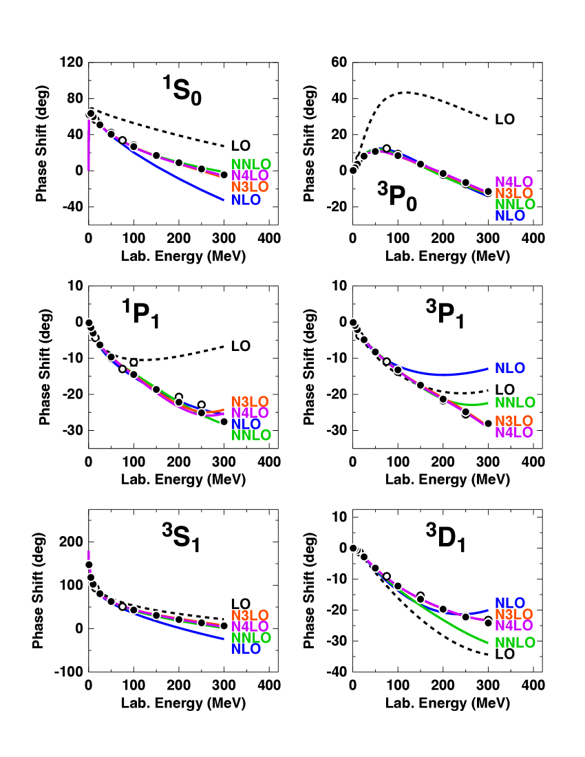
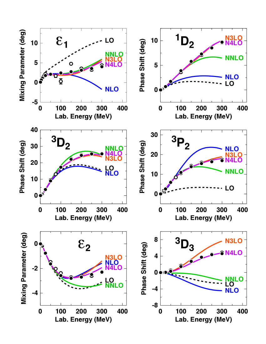
$NN$ potentials are then constructed order by order and the accuracy improves as the order increases. How well the chiral expansion converges in important lower partial waves is demonstrated in Figs. 9 and 10, where we show phase parameters for potentials developed through all orders from LO to N⁴LO [77].  These figures clearly reveal substantial improvements in the reproduction of the empirical phase shifts with increasing order.

The $\chi^{2}$/datum for the reproduction of the $NN$ data at various orders of chiral EFT are shown in Table 1 for different energy intervals below 290 MeV laboratory energy ($T_{\rm lab}$). The bottom line of Table 1 summarizes the essential results. For the close to 5000 $pp$ plus $np$ data below 290 MeV (pion-production threshold), the $\chi^{2}$/datum is 51.4 at NLO and 6.3 at NNLO. Note that the number of $NN$ contact terms is the same for both orders. The improvement is entirely due to an improved description of the 2PE contribution, which is responsible for the crucial intermediate-range attraction of the nuclear force. At NLO, only the uncorrelated 2PE is taken into account which is insufficient. From the classic meson-theory of nuclear forces [43] (Sec. 2), it is wellknown that $\pi$-$\pi$ correlations and nucleon resonances need to be taken into account for a realistic model of 2PE. As discussed, in the chiral theory, these contributions are encoded in the subleading $\pi N$ vertexes with LECs denoted by $c_{i}$, Eq. (26). These enter at NNLO and are the reason for the substantial improvements we encounter at that order.

To continue on the bottom line of Table 1, after NNLO, the $\chi^{2}$/datum then further improves to 1.63 at N³LO and, finally, reaches the almost perfect value of 1.15 at N⁴LO—a fantastic convergence.

Table 2: Two- and three-nucleon bound-state properties as predicted by $NN$ potentials at various orders of chiral EFT ($\Lambda=500$ MeV in all cases). (Deuteron: Binding energy $B_{d}$, asymptotic $S$ state $A_{S}$, asymptotic $D/S$ state $\eta$, structure radius $r_{\rm str}$, quadrupole moment $Q$, $D$-state probability $P_{D}$; the predicted $r_{\rm str}$ and $Q$ are without meson-exchange current contributions and relativistic corrections. Triton: Binding energy $B_{t}$.) $B_{d}$ is fitted, all other quantities are predictions. (From Ref. [77].)

	LO	NLO	NNLO	N3LO	N4LO	Empiricala
Deuteron
$B_{d}$ (MeV)	2.224575	2.224575	2.224575	2.224575	2.224575	2.224575(9)
$A_{S}$ (fm-1/2)	0.8526	0.8828	0.8844	0.8853	0.8852	0.8846(9)
$\eta$	0.0302	0.0262	0.0257	0.0257	0.0258	0.0256(4)
$r_{\rm str}$ (fm)	1.911	1.971	1.968	1.970	1.973	1.97507(78)
$Q$ (fm2)	0.310	0.273	0.273	0.271	0.273	0.2859(3)
$P_{D}$ (%)	7.29	3.40	4.49	4.15	4.10	—
Triton
$B_{t}$ (MeV)	11.09	8.31	8.21	8.09	8.08	8.48

^aSee Table XVIII of Ref. [35] for references; the empirical value for $r_{\rm str}$ is from Ref. [86].

The evolution of the deuteron properties from LO to N⁴LO of chiral EFT are shown in Table 2. In all cases, we fit the deuteron binding energy to its empirical value of 2.224575 MeV using the non-derivative ${}^{3}S_{1}$ contact. All other deuteron properties are predictions. Already at NNLO, the deuteron has converged to its empirical properties and stays there through the higher orders.

At the bottom of Table 2, we also show the predictions for the triton binding as obtained in 34-channel charge-dependent Faddeev calculations using only 2NFs. The results show smooth and steady convergence, order by order, towards a value around 8.1 MeV that is reached at the highest orders shown. This contribution from the 2NF will require only a moderate 3NF. The relatively low deuteron $D$-state probabilities ($\approx 4.1$% at N³LO and N⁴LO) and the concomitant generous triton binding energy predictions are a reflection of the fact that our $NN$ potentials are soft (which is, at least in part, due to their non-local character).

3.7 Nuclear many-body forces

Two-nucleon forces derived from chiral EFT have been applied, often successfully, in the many-body system. On the other hand, over the past several years we have learnt that, for some few-nucleon reactions and nuclear structure issues, 3NFs cannot be neglected. The most well-known cases are the so-called $A_{y}$ puzzle of $N$-$d$ scattering [87], the ground state of ¹⁰B [88], and the saturation of nuclear matter [89, 90, 91]. As we observed previously, the EFT approach generates consistent two- and many-nucleon forces in a natural way (cf. the overview given in Fig. 7). We now shift our focus to chiral three- and four-nucleon forces.

3.7.1 Three-nucleon forces

Weinberg [61] was the first to discuss nuclear three-body forces in the context of ChPT. Not long after that, the first 3NF at NNLO was derived by van Kolck [62].

For a 3NF, we have $A=3$ and $C=1$ and, thus, Eq. (32) implies

$$\nu=2+2L+\sum_{i}\Delta_{i}\,.$$ (50)

We will use this equation to analyze 3NF contributions order by order.

Next-to-leading order

The lowest possible power is obviously $\nu=2$ (NLO), which is obtained for no loops ($L=0$) and only leading vertices ($\sum_{i}\Delta_{i}=0$). As discussed by Weinberg [61] and van Kolck [62], the contributions from these diagrams vanish at NLO. So, the bottom line is that there is no genuine 3NF contribution at NLO. The first non-vanishing 3NF appears at NNLO.

Next-to-next-to-leading order

The power $\nu=3$ (NNLO) is obtained when there are no loops ($L=0$) and $\sum_{i}\Delta_{i}=1$, i.e., $\Delta_{i}=1$ for one vertex while $\Delta_{i}=0$ for all other vertices. There are three topologies which fulfill this condition, known as the 2PE, 1PE, and contact graphs [62, 63] (Fig. 11).

The 2PE 3N-potential is derived to be

$$V^{\rm 3NF}_{\rm 2PE}=\left(\frac{g_{A}}{2f_{\pi}}\right)^{2}\frac{1}{2}\sum_{i\neq j\neq k}\frac{(\vec{\sigma}_{i}\cdot\vec{q}_{i})(\vec{\sigma}_{j}\cdot\vec{q}_{j})}{(q^{2}_{i}+m^{2}_{\pi})(q^{2}_{j}+m^{2}_{\pi})}\;F^{ab}_{ijk}\;\tau^{a}_{i}\tau^{b}_{j}$$ (51)

with $\vec{q}_{i}\equiv\vec{p_{i}}^{\prime}-\vec{p}_{i}$, where $\vec{p}_{i}$ and $\vec{p_{i}}^{\prime}$ are the initial and final momenta of nucleon $i$, respectively, and

$$F^{ab}_{ijk}=\delta^{ab}\left[-\frac{4c_{1}m^{2}_{\pi}}{f^{2}_{\pi}}+\frac{2c_{3}}{f^{2}_{\pi}}\;\vec{q}_{i}\cdot\vec{q}_{j}\right]+\frac{c_{4}}{f^{2}_{\pi}}\sum_{c}\epsilon^{abc}\;\tau^{c}_{k}\;\vec{\sigma}_{k}\cdot[\vec{q}_{i}\times\vec{q}_{j}]\;.$$ (52)

It is interesting to observe that there are clear analogies between this force and earlier 2PE 3NFs already proposed decades ago, particularly the Fujita-Miyazawa [92] and the Tucson-Melbourne (TM) [93] forces.

Figure 11: The three-nucleon force at NNLO with (a) 2PE, (b) 1PE, and (c) contact diagrams. Notation as in Fig. 7.

The 2PE 3NF does not introduce additional fitting constants, since the LECs $c_{1}$, $c_{3}$, and $c_{4}$ are already present in the 2PE 2NF.

The other two 3NF contributions shown in Fig. 11 are easily derived by taking the last two terms of the $\Delta=1$ Langrangian, Eq. (26), into account. The 1PE contribution is

$$V^{\rm 3NF}_{\rm 1PE}=-D\;\frac{g_{A}}{8f^{2}_{\pi}}\sum_{i\neq j\neq k}\frac{\vec{\sigma}_{j}\cdot\vec{q}_{j}}{q^{2}_{j}+m^{2}_{\pi}}(\mbox{\boldmath$\tau$}_{i}\cdot\mbox{\boldmath$\tau$}_{j})(\vec{\sigma}_{i}\cdot\vec{q}_{j})$$ (53)

and the 3N contact potential is given by

$$V^{\rm 3NF}_{\rm ct}=E\;\frac{1}{2}\sum_{i\neq j\neq k}\mbox{\boldmath$\tau$}_{i}\cdot\mbox{\boldmath$\tau$}_{j}\;.$$ (54)

These 3NF potentials introduce two additional constants, $D$ and $E$, which can be constrained in more than one way. One may use the triton binding energy and the $nd$ doublet scattering length ${}^{2}a_{nd}$ [63] or an optimal global fit of the properties of light nuclei [94]. Alternative choices include the binding energies of ³H and ⁴He [95] or the binding energy of ³H and the point charge radius of ⁴He [96]. Another method makes use of the triton binding energy and the Gamow-Teller matrix element of tritium $\beta$-decay [97]. When the values of $D$ and $E$ are determined, the results for other observables involving three or more nucleons are true theoretical predictions.

Applications of the leading 3NF include few-nucleon reactions [63, 98, 99], structure of light- and medium-mass nuclei [100, 101, 102, 103, 104, 105, 106], and infinite matter [107, 96, 108, 109, 89, 90, 91], often with satisfactory results. Some problems, though, remain unresolved, such as the well-known ‘$A_{y}$ puzzle’ in nucleon-deuteron scattering [87, 63]. Predictions which employ only 2NFs underestimate the analyzing power in $p$-³He scattering to a larger degree than in $p$-$d$. Although the $p$-³He $A_{y}$ improves considerably (more than in the $p$-$d$ case) when the leading 3NF is included [99], the disagreement with the data is not fully removed. Also, predictions for light nuclei are not quite satisfactory.

In summary, the leading 3NF of ChPT is a remarkable contribution. It gives validation to, and provides a better framework for, 3NFs which were proposed already five decades ago; it alleviates existing problems in few-nucleon reactions and the spectra of light nuclei. Nevertheless, we still face several challenges. With regard to the 2NF, we have discussed earlier that it is necessary to go to order four or even five for convergence and high-precison predictions. Thus, the 3NF at N³LO must be considered simply as a matter of consistency with the 2NF sector. At the same time, one hopes that its inclusion may result in further improvements with the aforementioned unresolved problems.

Figure 12: Leading one-loop 3NF diagrams at N³LO. We show one representative example for each of five topologies, which are: (a) 2PE, (b) 1PE-2PE, (c) ring, (d) contact-1PE, (e) contact-2PE. Notation as in Fig. 7.

Next-to-next-to-next-to-leading order

At N³LO, there are loop and tree diagrams. For the loops (Fig. 12), we have $L=1$ and, therefore, all $\Delta_{i}$ have to be zero to ensure $\nu=4$. Thus, these one-loop 3NF diagrams can include only leading order vertices, the parameters of which are fixed from $\pi N$ and $NN$ analysis. The diagrams have been evaluated by the Bochum-Bonn group [110, 111]. The long-range part of the chiral N³LO 3NF has been tested in the triton and in three-nucleon scattering [112] yielding only moderate effects. The long- and short-range parts of this force have been used in neutron matter calculations (together with the N³LO 4NF) producing relatively large contributions from the 3NF [113, 114]. Thus, the ultimate assessment of the N³LO 3NF is still outstanding and will require more few- and many-body applications.

The 3NF at N⁴LO

Figure 13: Sub-leading one-loop 3NF diagrams which appear at N⁴LO with topologies similar to Fig. 12. Notation as in Fig. 7.

Figure 14: 3NF tree graphs at N⁴LO ($\nu=5$) denoted by: (a) 2PE, (b) 1PE-contact, and (c) contact. Notation as in Fig. 7.

In the meantime, one may go ahead and look at the next order of 3NFs, which is N⁴LO or $\nu=5$. The loop contributions that occur at this order are obtained by replacing in the N³LO loops one vertex by a $\Delta_{i}=1$ vertex (with LEC $c_{i}$), Fig. 13, which is why these loops may be more sizable than the N³LO loops. The 2PE, 1PE-2PE, and ring topologies have been evaluated [59, 68] so far. In addition, we have three ‘tree’ topologies (Fig. 14), which include a new set of 3N contact interactions that has recently been derived by the Pisa group [69]. Contact terms are typically simple (as compared to loop diagrams) and their coefficients are essentially free. Therefore, it is an attractive project to test some terms (in particular, the spin-orbit terms) of the N⁴LO contact 3NF in calculations of few-body reactions (specifically, the $p$-$d$ and $p$-³He $A_{y}$), which is under way [115].

3.7.2 Four-nucleon forces

For connected ($C=1$) $A=4$ diagrams, Eq. (32) yields

$$\nu=4+2L+\sum_{i}\Delta_{i}\,.$$ (55)

We then see that the first (connected) non-vanishing 4NF is generated at $\nu=4$ (N³LO), with all vertices of leading type, Fig. 15. This 4NF has no loops and introduces no novel parameters [116].

For a reasonably convergent series, terms of order $(Q/\Lambda_{\chi})^{4}$ should be small and, therefore, chiral 4NF contributions are expected to be very weak. This has been confirmed in calculations of the energy of ⁴He [117] and neutron matter [113].

The effects of the leading chiral 4NF in symmetric nuclear matter and pure neutron matter have been worked out by Kaiser et al. [118, 119].

Figure 15: Leading four-nucleon force at N³LO.

4 Phase IV (2020 – 2050?) Future: EFT Based Models(?)

One of the most fundamental aims in theoretical nuclear physics is to understand nuclear structure and reactions in terms of the basic forces between nucleons. Research pursuing this goal has two major ingredients: nuclear forces and quantum many-body theory.

As demonstrated in the previous section, the advantage of chiral EFT is that it generates the forces needed (two- and many-body forces) on an equal footing and in a systematic way (namely, order by order), while at the same time improving the precision of the predictions and allowing for reliable uncertainty quantifications (cf. Sec. V of Ref. [77]).

Concerning the second ingredient, during the past two decades, there has been great progress in the development and refinement of diverse many-body methods. Among them are the no-core shell model [102], coupled cluster theory [104], self-consistent Green’s functions [120], quantum Monte Carlo [121], and the in-medium similarity renormalization group method [122].

In the pursuit of the fundamental aim, a large number of applications of the chiral $NN$ potentials (usually up to N³LO) together with chiral 3NFs (generally just at NNLO) have been conducted. These investigations include few-nucleon reactions [63, 98, 99, 112], structure of light- and medium-mass nuclei [100, 101, 102, 103, 104, 105, 106], and infinite matter [107, 96, 108, 109, 89, 90, 91]. Although satisfactory predictions have been obtained in many cases, persistent problems continue to pose serious challenges, such as the well-known ‘$A_{y}$ puzzle’ of nucleon-deuteron scattering [87, 63, 99, 112]. For intermediate mass nuclei, we are faced with systematic overbinding [123] and a “radius problem” [124].

Naturally, one would suspect missing 3NFs as the most likely mechanism to solve the open questions, particularly, since most current calculations include 3NFs only at NNLO. However, the 3NFs at N³LO [110, 111] and N⁴LO [59, 68] (cf. Sec. 3.7.1) are so terribly complicated that including them all is not a realistic task. Thus, it appears that chiral EFT, when pursued consistently, may become unmanageable.

In view of this frustrating situation, an alternative culture is emerging that breaks with conventional practises. As outlined in Secs. 3.6.4 and 3.7.1, in the conventional approach, the $\pi N$ LECs are fixed by the $\pi N$ data, the $NN$ contacts by the two-nucleon data, and the 3N LECs by three-nucleon data. All applications of these forces in systems with $A>3$ are then predictions. In the unconventional approach, with which presently some researchers are experimenting (see e.g., Refs. [125, 126, 127]), the 2NFs and 3NFs are treated on the manageable NNLO level, and the $\pi N$, NN, and 3NF LECs are determined simultaneously. Furthermore, to ensure better results for intermediate-mass nuclei, the binding energies and radii of few-nucleon systems and selected isotopes of oxygen and, in some cases, even carbon are included in the optmization procedure. The inclusion of selected spectra of light nuclei in the optimization is also contemplated. These interactions then predict binding energies and radii of nuclei up to ⁴⁰Ca much better [125]. However, in most of these models, the $NN$ data are reproduced only at very low energies. To justify this approach, it is argued that low-energy nuclear observables should be sensitive only to low-energy $NN$ properties. Predictive power and large extrapolations do not go together well, as small uncertainties in few-body systems get magnified in heavy nuclei. Therefore, in this philosophy [125], light nuclei are “predicted” by interpolation, heavy nuclei by modest extrapolation. The spirit of this culture is similar to the one of the nuclear mean-field and nuclear density functional theory. However, it needs to be stressed that approaches of this kind are models.

A dogma of chiral EFT is that a calculation is only meaningful if it includes all terms up to the given order (i.e., all 2NF, 3NF, and potentially 4NF contributions up to the given order). However, the combination of N³LO 2NFs and NNLO 3NFs has already become common practise. In the future, we expect that N⁴LO 2NFs are combined with selected (but not all) N⁴LO 3NF (contact) terms. Skillfully chosen combinations carry the potential to solve some puzzles that have been oustanding for 30 years, like the $Nd$ $A_{y}$ puzzle [115], and problems with some spectra of light and intermediate-mass nuclei. Since the 3NF terms at N³LO and N⁴LO are so numerous, selecting just a few of them that show potential will be the best one can do for a while (if not for ever).

Thus, chiral EFT may ultimately suffer the same fate as meson theory. As explained in Sections 1 and 2, meson theory was originally (Phase I) designed to be a quantum field theory, but later (Phase II) had to be demoted to the level of a model (a very successful model, though). During the current Phase III, the main selling point has been that chiral EFT is a theory and not just a model and, therefore, its dogmatic use has been pushed. However, in analogy to what historically happened to meson theory, during the next phase (namely, Phase IV), we may have to resign ourselves to chiral EFT based models (that may potentially have great success).

The history of nuclear forces clearly shows a pattern of 30-year phases. Whether these cycles will go on forever or whether Phase IV will be the last one, we will know Anno Domini 2050.

References

- [1] J. Chadwick, Proc. Roy. Soc. (London) A136, 692 (1932).
- [2] L. M. Brown and H. Rechenberg, The Origin of the Concept of Nuclear Forces (IOP Publishing, Bristol and Philadelphia, 1996).
- [3] W. Heisenberg, Z. Phys. 77, 1; 78, 156 (1932); 80, 587 (1933).
- [4] H. Yukawa, Proc. Phys. Math. Soc. Japan 17, 48 (1935).
- [5] E. Fermi, Z. Phys. 88, 161 (1934).
- [6] S. H. Neddermeyer and C. D. Anderson, Phys. Rev. 51, 884 (1937).
- [7] H. Yukawa and S. Sakata, Proc. Phys. Math. Soc. Japan 19, 1084 (1937).
- [8] N. Kemmer, Proc. Roy. Soc. (London) A166, 127 (1938).
- [9] C. M. G. Lattes, G. P. S. Occhialini, and C. F. Powell, Nature 160, 453, 486 (1947).
- [10] E. Gardner and C. M. G. Lattes, Science 107, 270 (1948).
- [11] M. Taketani, S. Machida, and S. Onuma, Prog. Theor. Phys. (Kyoto) 7, 45 (1952).
- [12] K. A. Brueckner and K. M. Watson, Phys. Rev. 90, 699; 92, 1023 (1953).
- [13] R. E. Marshak, Meson Physics (New York, 1952).
- [14] S. S. Schweber, H. A. Bethe, and F. de Hoffmann, Mesons and Fields, Volume I Fields (Row, Peterson and Company, Evanston, IL, 1955).
- [15] H. A. Bethe, and F. de Hoffmann, Mesons and Fields, Volume II Mesons (Row, Peterson and Company, Evanston, IL, 1955).
- [16] M. J. Moravcsik, The Two-Nucleon Interaction (Clarendon Press, Oxford, 1963).
- [17] O. Chamberlain, E. Segre, R. D. Tripp, C. Wiegand and T. Ypsilantis, Phys. Rev. 105, 288 (1957).
- [18] H. P. Stapp, T. J. Ypsilantis and N. Metropolis, Phys. Rev. 105, 302 (1957).
- [19] J. J. Sakurai, Phys. Rev. 119, 1784 (1960).
- [20] G. Breit, Phys. Rev. 120, 287 (1960).
- [21] Y. Nambu, Phys. Rev. 106, 1366 (1957).
- [22] W. R. Frazer and J. R. Fulco, Phys. Rev. Lett. 2, 365 (1959); Phys. Rev. 117, 1609 (1960).
- [23] B. C. Maglic et al., Phys. Rev. Lett. 7, 178 (1961).
- [24] A. R. Erwin et al., Phys. Rev. Lett. 6, 628 (1961).
- [25] M. J. Moravcsik, Rep. Prog. Phys. 35, 587 (1972).
- [26] C Patrignani et al (Particle Data Group), Chin. Phys. C 40, 100001 (2016).
- [27] R. Machleidt, Adv. Nucl. Phys. 19, 189 (1989).
- [28] R. A. Bryan and B. L. Scott, Phys. Rev. 135 (1964) B434; 177 (1969) 1435.
- [29] A. E. S. Green, M. H. MacGregor and R. Wilson, Rev. Mod. Phys. 39 (1967) 495.
- [30] M. M. Nagels, T. A. Rijken, and J. J. de Swart, Phys. Rev. D 17, 768 (1978).
- [31] V. G. J. Stoks, R. A. M. Klomp, C. P. F. Terheggen, and J. J. de Swart, Phys. Rev. C 49, 2950 (1994).
- [32] A. Gersten, R. Thompson, and A. E. S. Green, Phys. Rev. D 3, 2076 (1971). G. Schierholz, Nucl. Phys. B40, 335 (1972). J. Fleischer and J. A. Tjon, Nucl. Phys. B84, 375 (1975); Phys. Rev. D 24, 87 (1980).
- [33] K. Erkelenz, Phys. Reports 13C, 191 (1974).
- [34] K. Holinde and R. Machleidt, Nucl. Phys. A247, 495 (1975); ibid. A256, 479 (1976).
- [35] R. Machleidt, Phys. Rev. C 63 024001 (2001).
- [36] M. Chemtob, J. W. Durso, and D. O. Riska, Nucl. Phys. B38, 141 (1972); A. D. Jackson, D. O. Riska. and B. Verwest, Nucl. Phys. A249, 397 (1975).
- [37] G. E. Brown and A. D. Jackson, The Nucleon-Nucleon Interaction (North-Holland, Amsterdam, 1976).
- [38] W. N. Cottingham and R. Vinh Mau, Phys. Rev. 130, 735 (1963).
- [39] W. N. Cottingham, M. Lacombe, B. Loiseau, J. M. Richard, and R. Vinh Mau, Phys. Rev. D 8, 800 (1973); R. Vinh Mau, J. M. Richard, B. Loiseau, M. Lacombe, and W. N. Cottingham, Phys. Lett. B 44, 1 (1973).
- [40] M. Lacombe, B. Loiseau, J. M. Richard, R. Vinh Mau, J. Côté, P. Pirès, and R. de Tourreil, Phys. Rev. C 21, 861 (1980).
- [41] R. Vinh Mau, in Mesons in Nuclei, Vol. I, eds. M. Rho and D. H. Wilkinson (North-Holland, Amsterdam, 1979) pp.151-196.
- [42] M. H. Partovi and E. L. Lomon, Phys. Rev. D 2, 1999 (1970).
- [43] R. Machleidt, K. Holinde, and Ch. Elster, Phys. Reports 149, 1 (1987).
- [44] R. B. Wiringa, V. G. J. Stoks, and R. Schiavilla, Phys. Rev. C 51, 38 (1995).
- [45] D. R. Entem, F. Fernandez, and A. Valcarce, Phys. Rev. C 62, 034002 (2000), and references to earlier work therein.
- [46] K. Orginos, A. Parreño, M. J. Savage, S. R. Beane, E. Chang, and W. Detmold, Phys. Rev. D 92, 114512 (2015).
- [47] T. Hatsuda, J. Phys. Conf. Ser. 381, 012020 (2012).
- [48] S. Weinberg, Physica 96A, 327 (1979).
- [49] J. Gasser and H. Leutwyler, Ann. Phys. 158, 142 (1984); Nucl. Phys. B250, 465 (1985).
- [50] J. Gasser, M. E. Sainio, and A. Švarc, Nucl. Phys. B307, 779 (1986).
- [51] S. Weinberg, Phys. Lett. B251, 288 (1990).
- [52] S. Weinberg, Nucl. Phys. B363, 3 (1991).
- [53] S. Weinberg, “What is Quantum Field Theory, and What Did We Think It Is?”, arXiv:hep-th/9702027.
- [54] S. Weinberg, “Effective Field Theory, Past and Future”, arXiv:0908:1964 [hep-th].
- [55] R. Machleidt and D. R. Entem, Phys Reports 503, 1 (2011).
- [56] S. Scherer, Adv. Nucl. Phys. 27, 277 (2003).
- [57] S. Coleman, J. Wess, and B. Zumino, Phys. Rev. 177, 2239 (1969); C. G. Callan, S. Coleman, J. Wess, and B. Zumino, ibid. 177, 2247 (1969).
- [58] N. Fettes, U.-G. Meißner, M. Mojžiš, and S. Steininger, Ann. Phys. (N.Y.) 283, 273 (2000); 288, 249 (2001).
- [59] H. Krebs, A. Gasparyan, and E. Epelbaum, Phys. Rev. C 85, 054006 (2012).
- [60] C. Ordóñez, L. Ray, and U. van Kolck, Phys. Rev. C 53, 2086 (1996).
- [61] S. Weinberg, Phys. Lett. B 295, 114 (1992).
- [62] U. van Kolck, Phys. Rev. C 49, 2932 (1994).
- [63] E. Epelbaum, A. Nogga, W. Glöckle, H. Kamada, U.-G. Meißner, and H. Witala, Phys. Rev. C 66, 064001 (2002).
- [64] N. Kaiser, Phys. Rev. C 61, 014003 (2000).
- [65] N. Kaiser, Phys. Rev. C 62, 024001 (2000).
- [66] D. R. Entem and R. Machleidt, Phys. Rev. C 68, 041001 (2003).
- [67] D. R. Entem, N. Kaiser, R. Machleidt, and Y. Nosyk, Phys. Rev. C 91, 014002 (2015).
- [68] H. Krebs, A. Gasparyan, and E. Epelbaum, Phys. Rev. C 87, 054007 (2013).
- [69] L. Girlanda, A. Kievsky, M. Viviani, Phys. Rev. C 84, 014001 (2011).
- [70] D. R. Entem, N. Kaiser, R. Machleidt, and Y. Nosyk, Phys. Rev. C 92, 064001 (2015).
- [71] D. R. Entem and R. Machleidt, unpublished.
- [72] V. G. J. Stoks, R. A. M. Klomp, M. C. M. Rentmeester, and J. J. de Swart, Phys. Rev. C 48, 792 (1993).
- [73] W. J. Briscoe, I. I. Strakovsky, and R. L. Workman, SAID Partial-Wave Analysis Facility, Data Analysis Center, The George Washington University, solution SP07 (Spring 2007).
- [74] R. Blankenbecler and R. Sugar, Phys. Rev. 142, 1051 (1966).
- [75] D. B. Kaplan, M. Savage, and M. B. Wise, Nucl. Phys. B478, 629 (1996); Phys. Lett. B424, 390 (1998); Nucl. Phys. B534, 329 (1998).
- [76] M. Hoferichter, J. Ruiz de Elvira, B. Kubis, and U.-G. Meißner, Phys. Rev. Lett. 115, 192301 (2015); Phys. Rep. 625, 1 (2016).
- [77] D. R. Entem, R. Machleidt, and Y. Nosyk, Phys. Rev. C 96, 024004 (2017).
- [78] E. Epelbaum, W. Glöckle, and U.-G. Meißner, Nucl. Phys. A747, 362 (2005).
- [79] E. Epelbaum, H. Krebs, U.-G. Meißner, Eur. Phys. J. A51, 53 (2015).
- [80] E. Epelbaum, H. Krebs, U.-G. Meißner, Phys. Rev. Lett. 115, 122301 (2015).
- [81] A. Ekstrőm et al., Phys. Rev. Lett. 110, 192502 (2013).
- [82] A. Gezerlis, I. Tews, E. Epelbaum, M. Freunek, S. Gandolfi, K. Hebeler, A. Nogga, and A. Schwenk, Phys. Rev. C 90, 054323 (2014).
- [83] M. Piarulli, L. Girlanda, R. Schiavilla, R. Navarro Pérez, J. E. Amaro, and E. Ruiz Arriola, Phys. Rev. C 91, 024003 (2015).
- [84] M. Piarulli, L. Girlanda, R. Schiavilla, A. Kievsky, A. Lovato, L. E. Marcucci, Steven C. Pieper, M. Viviani, and R. B. Wiringa, Phys. Rev. C 94, 054007 (2016).
- [85] R. Navarro Pérez, J. E. Amaro, and E. Ruiz Arriola, Phys. Rev. C 91, 054002 (2015), and references to the comprehensive work by the Granada group therein.
- [86] U. D. Jentschura, A. Matveev, C. G. Parthey, J. Alnis, R. Pohl, Th. Udem, N. Kolachevsky, and T. W. Ha̋nsch, Phys. Rev. A 83, 042505 (2011).
- [87] D. R. Entem, R. Machleidt, and H. Witala, Phys. Rev. C 65, 064005 (2002).
- [88] E. Caurier, P. Navratil, W. E. Ormand, and J. P. Vary, Phys. Rev. C 66, 024314 (2002).
- [89] L. Coraggio, J. W. Holt, N. Itaco, R. Machleidt, L. E. Marcucci, and F. Sammarruca, Phys. Rev. C 89, 044321 (2014).
- [90] F. Sammarruca, L. Coraggio, J. W. Holt, N. Itaco, R. Machleidt, and L. E. Marcucci, Phys. Rev. C 91, 054311 (2015).
- [91] R. Machleidt and F. Sammarruca, Phys. Scr. 91, 083007 (2016).
- [92] J.-I. Fujita and H. Miyazawa, Prog. Theor. Phys. 17, 360 (1957).
- [93] S. A. Coon, M. D. Scadron, P. C. McNamee, B. R. Barrett, D. W. E. Blatt. and B. H. J. McKeller, Nucl. Phys. A317, 242 (1979).
- [94] P. Navratil, Few Body Syst. 41, 117 (2007).
- [95] A. Nogga, P. Navratil, B. R. Barrett, and J. P. Vary, Phys. Rev. C 73, 064002 (2006).
- [96] K. Hebeler, S. K. Bogner, R. J. Furnstahl, A. Nogga, and A. Schwenk, Phys. Rev. C 83, 031301(R) (2011).
- [97] L. E. Marcucci, A. Kievsky, S. Rosati, R. Schiavilla, and M. Viviani, Phys. Rev. Lett. 108, 052502 (2012).
- [98] P. Navratil, R. Roth, and S. Quaglioni, Phys. Rev. C 82, 034609 (2010).
- [99] M. Viviani, L. Girlanda, A. Kievsky, and L. E. Marcucci, Phys. Rev. Lett. 111, 172302 (2013).
- [100] H. Hagen, M. Hjorth-Jensen, G. R. Jansen, R. Machleidt, and T. Papenbrock, Phys. Rev. Lett. 108, 242501 (2012).
- [101] H. Hagen, M. Hjorth-Jensen, G. R. Jansen, R. Machleidt, and T. Papenbrock, Phys. Rev. Lett. 109, 032502 (2012).
- [102] B. R. Barrett, P. Navratil, and J. P. Vary, Prog. Part. Nucl. Phys. 69, 131 (2013).
- [103] H. Hergert, S. K. Bogner, S. Binder, A. Calci, J. Langhammer, R. Roth, and A. Schwenk, Phys. Rev. C 87, 034307 (2013).
- [104] G. Hagen, T. Papenbrock, M. Hjorth-Jensen, and D. J. Dean, Rept. Prog. Phys. 77, 096302 (2014).
- [105] J. Simonis, S. R. Stroberg, K. Hebeler, J. D. Holt, and A. Schwenk, Phys. Rev. C 96, 014303 (2017)
- [106] T. D. Morris, J. Simonis, S. R. Stroberg, C. Stumpf, G. Hagen, J. D. Holt, G. R. Jansen, T. Papenbrock, R. Roth, and A. Schwenk, “Structure of the lightest tin isotopes”, arXiv:1709.02786 [nucl-th].
- [107] K. Hebeler and A. Schwenk, Phys. Rev. C 82, 014314 (2010).
- [108] G. Hagen, T. Papenbrock, A. Ekstrőm, K. A. Wendt, G. Baardsen, S. Gandolfi, M. Hjorth-Jensen, and C. J. Horowitz, Phys. Rev. C 89, 014319 (2014).
- [109] L. Coraggio, J. W. Holt, N. Itaco, R. Machleidt, and F. Sammarruca, Phys. Rev. C 87, 014322 (2013).
- [110] V. Bernard, E. Epelbaum, H. Krebs, and Ulf-G. Meißner, Phys. Rev. C 77, 064004 (2008).
- [111] V. Bernard, E. Epelbaum, H. Krebs, and Ulf-G. Meißner, Phys. Rev. C 84, 054001 (2011).
- [112] J. Golak et al., Eur. Phys. J. A 50, 177 (2014).
- [113] T. Krűger, I. Tews, K Hebeler, and A. Schwenk, Phys. Rev. C 88, 025802 (2013).
- [114] C. Drischler, A. Carbone, K. Hebeler, and A. Schwenk, Phys. Rev. C 94, 054307 (2016).
- [115] L. Girlanda, A. Kievsky, M. Viviani, and L. E. Marcucci, PoS (CD15), 103 (2016).
- [116] E. Epelbaum, Eur. Phys. J. A34, 197 (2007).
- [117] D. Rozpedzik, J. Golak, R. Skibinski, H. Witala, W. Glöckle, E. Epelbaum, A. Nogga, and H. Kamada, Acta Phys. Polon. B37, 2889 (2006); arXiv:nucl-th/0606017.
- [118] N. Kaiser, Eur. Phys. J. A 48, 135 (2012).
- [119] N. Kaiser and R. Milkus, Eur. Phys. J. A 52, 4 (2016).
- [120] V. Somà, A. Cipollone, C. Barbieri, P. Navratil, and T. Duget, Phys. Rev. C 89, 061301(R) (2014).
- [121] J. Carlson, S. Gandolfi, F. Pederiva, S. C. Pieper, R. Schiavilla, K. E. Schmidt, and R. B. Wiringa, Rev. Mod. Phys. 87, 1067 (2015).
- [122] H. Hergert, S. K. Bogner, T. D. Morris, A. Schwenk, and K. Tsukiyama, Phys. Rep. 621, 165 (2016).
- [123] S. Binder, J. Langhammer, A. Calci, and R. Roth, Phys. Lett. B736, 119 (2014).
- [124] V. Lapoux, V. Somà, C. Barbieri, H. Hergert, J. D. Holt, and S. R. Stroberg, Phys. Rev. Lett. 117, 052501 (2016).
- [125] A. Ekstrőm et al., Phys. Rev. C 91, 051301 (2015).
- [126] B. D. Carlsson et al., Phys. Rev. X 6, 011019 (2016).
- [127] A. Ekstrőm et al., “Delta isobars and nuclear saturation”, arXiv:1707.09028 [nucl-th].