Diffusion-Limited Reactions in Nanoscale Electronics

Abstract

A partial differential equation (PDE) was developed to describe time-dependent ligand-receptor interactions for applications in biosensing using field effect transistors (FET). The model describes biochemical interactions at the sensor surface (or biochemical gate) located at the bottom of a solution-well, which result in a time-dependent change in the FET conductance. It was shown that one can exploit the disparate length scales of the solution-well and biochemical gate to reduce the coupled PDE model to a single nonlinear integrodifferential equation (IDE) that describes the concentration of reacting species. Although this equation has a convolution integral with a singular kernel, a numerical approximation was constructed by applying the method of lines. The need for specialized quadrature techniques was obviated and numerical evidence strongly suggests that this method achieves first-order accuracy. Results reveal a depletion region on the biochemical gate, which non-uniformly alters the surface potential of the semiconductor.

1 Introduction

The ability to tailor therapies to individuals or specific subsets of a population to deliver personalized care has the potential to fundamentally remake healthcare delivery. The most promising therapeutic candidates for such targeted care are new classes of biologic drugs based on naturally occurring molecules, made possible due to rapid advances in genomics and proteomics [9, 23]. Importantly, such therapies can be safer and yield better outcomes at lower doses when treating debilitating conditions such as diabetes, Alzheimer’s disease, or certain cancers [2, 7]. The widespread use of personalized care is currently limited by our ability to routinely measure pathology in individuals including biomarkers, metabolites, tissue histology, and gene expression. Moreover, existing clinical diagnostics are cumbersome, require specialized facilities, can take days to weeks to perform, and are in many cases prohibitively expensive. This has led to the development of new portable detection tools including antibody-based lateral flow assays [8, 16], microelectromechanical sensor (MEMS) based resonators that can detect binding of biomarkers to the sensor surface [12, 13, 18, 20], surface plasmon resonance [14, 24], ring cavity resonators [1, 4, 21], and electronic measurements with field effect transistors (FET) [6, 17, 19, 25]. The latter are particularly well-suited for biomarker measurements due their high charge sensitivity and direct signal transduction, allowing label-free measurements at physiological concentrations. Furthermore, by leveraging semi-conductor processing techniques, measurements with FETs can be made massively parallel, cost-effective, and portable.

A FET is a three-terminal device represented in Figure 1.1. A semiconductor channel between the source and drain terminals conducts a current that is strongly modulated by an electrostatic potential applied to the gate. Biomarkers in aqueous solution exhibit a well-defined electrostatic surface potential [5, 11] arising from charged hydrophilic residues that interact with water. When these molecules adsorb to the FET biochemical gate, they strongly modulate the channel current proportional to the magnitude of their surface potential. This allows FETs to be used to detect and quantify adsorbed biomarkers in solution. Furthermore, functionalizing the FET, by attaching molecules to the gate surface that have a high inherent affinity for biomarkers of interest (see Figure 1.1), allows measurements with high specificity that are tailored to one or more biomarkers of interest.

Figure 1.1: Schematic of biomarker measurements with a field effect transistor (FET). Ligand molecules injected at the top of the solution-well diffuse and bind with receptors immobilized on the FET biochemical gate. This schematic is not drawn to scale. In particular, the width of the solution-well is of on the order of millimeters, and substantially larger than the size of the biochemical gate, which spans micrometers. See Table 2.1 for exact parameter values.

An accurate and dynamical model of receptor ligand interactions at the biochemical gate is a critical component in maximizing the sensitivity of FET-based measurements. Specifically, quantitative descriptions of the distribution of adsorbed ligands and their surface potentials can be combined with a model of the semi-conductor physics to allow predictions of the measured signal. This in turn can be used to optimize sensor design, particularly the geometry of the biochemical gate. Of particular interest is a quantitative description of the coupling between bound ligand evolution and diffusion. To the authors’ knowledge this is a previously unexplored area of mathematical inquiry, though Poisson-Boltzman approaches to model sensor physics have been explored. For example in [10] Heitzinger et al. use the Poisson-Boltzman equation to develop a multiple-scale model for the electric potential distribution within semiconductors of planar and nanowire field-effect biosensors. Therein, the authors model these devices using three layers: a semiconductor layer, a dielectric layer, and a discrete layer of biomolecules immobilized on the dieletric layer. Homogenization techniques are employed to reconcile the biomolecule length scale with the semiconductor length scale, and interface conditions for the biomolecule-dielectric interface are derived. It must be noted that there are several important differences between [10] and the present manuscript. Perhaps the most important is that while [10] focuses on the electric potential distribution within the semiconductor channel, the present manuscript models the coupling between reaction and diffusion. Furthermore, while the authors of [10] model the biomolecule layer with a discrete number of biomolecules and use homogenization techniques, in the present manuscript a continuum perspective is presented. Finally, [10] assumes a steady distribution of biomolecules on the dielectric layer, while the present manuscript concerns the time-evolution of $B(x,t)$, which is experimentally measurable.

The authors of and [15] employ the one-dimensional Poisson-Boltzman equation to model the electrostatic potential from a layer of biological macromolecules on the biochemical gate of a metal-oxide-semiconductor transistor. In contrast, [3] uses a three-dimensional model of the electric potential in semiconductor channel, and couples the aqueous and semiconductor regions through interface conditions obtained from Monte-Carlo simulations, which provide an estimate of the charge distribution from adsorbed biomolecules on the biochemical gate.

In [22] Heitzinger, Mauser, and Ringhofer calculate numerical values for the kinetic parameters governing adsorption and desorption processes of $\mathrm{CO}$ at a $\mathrm{SnO}{}_{2}$ single-nanowire gas sensor. The authors adopt a continuum perspective by modeling surface reactions on a single-nanowire gas sensor through a set of differential equations. However, in [22] the authors simply apply the well-stirred kinetics approximation in which gaseous carbon monoxide transport is completely divorced from adsorption and desorption processes at the surface. This reduces their model to a set of nonlinear ordinary differential equations (ODE), which can be used to estimate kinetic rate constants involved in the reaction of interest.

In the present manuscript a quantitative description of the coupling between reaction and diffusion in FETs is developed. In particular, we consider the experimentally relevant limit of very low ligand concentrations—i.e., on the order of pico- to femtomolar concentrations—and very fast assocation rates. This problem is particularly challenging due to the disparate time and length scales involved. For example, the length scales span three orders of magnitude, ranging from order of millimeters for the solution-well to micrometers for the biochemical gate. Combining this fact with the diffusion-limited nature of the kinetics under consideration leads to the conclusion that the time-evolution of the reacting species concentration depends heavily on a diffusive boundary layer near the surface.

In Section 2 a mathematical modeled is developed that describe diffusion of ligand molecules through the solution-well onto the biochemical gate. In Subsection 2.1 the governing equations are presented, and it is shown that there are multiple time and length scales associated with the experiment. In Subsection 2.2, complex analysis techniques are employed to reduce the coupled PDE system to a single nonlinear integrodifferential equation (IDE) for the reacting species concentration. A quadrature-free numerical solution based on the method of lines is developed in Section 3, where it is shown that this method achieves first-order accuracy despite the presence of a convolution integral with a singular kernel. Results and their physical interpretations are discussed in Section 4, and concluding remarks are given in Section 5.

2 Governing Equations

2.1 Mathematical Model

Consider the geometry in Figure 1.1, and a rectangular domain, $(\widetilde{x},\widetilde{y})\in\ [0,\widetilde{L}]\times[0,\widetilde{H}]$, with the origin $(0,0)$ located at the lower-left corner of the well. The parameters $\widetilde{L}$ and $\widetilde{H}$ are the height and length of the well respectively; for parameter values see Table 2.1. Throughout the manuscript tildes are used to denote dimensional quantities. Receptors are confined to the biochemical gate, which occupies the very narrow region $(\widetilde{x},\widetilde{y})\in[-\widetilde{l}_{\mathrm{s}}/2+\widetilde{L}/2,\ \widetilde{L}/2+\widetilde{l}_{\mathrm{s}}]\times 0=[\widetilde{x}_{\mathrm{min}},\widetilde{x}_{\mathrm{max}}]\times 0$, where $\widetilde{l}_{\mathrm{s}}$ denotes length of the biochemical gate and $[\widetilde{x}_{\mathrm{min}},\widetilde{x}_{\mathrm{max}}]:=[-\widetilde{l}_{\mathrm{s}}/2+\widetilde{L}/2,\ \widetilde{L}/2+\widetilde{l}_{\mathrm{s}}]$. It is important to note that while the length scale of the well is on the order of millimeters, the length scale of the biochemical gate is on the order of micrometers.

Table 2.1: Bounds for dimensional and dimensionless parameters are given below.

Dimensional Parameters Dimensionless Parameters Parameter Range Parameter Range $\widetilde{D}\ (\mathrm{cm}^{2}/\mathrm{s})$ $10^{-6}$ $D_{\mathrm{w}}$ $2.5\times 10^{-2}$ to $2.5\times 10^{2}$ $\widetilde{k}_{\mathrm{a}}\ (\mathrm{cm}^{3}\cdot(\mathrm{mol}\cdot\mathrm{s})^{-1})$ $10^{11}$ to $10^{12}$ $D$ $4\times 10^{3}$ to $4\times 10^{7}$ $\widetilde{k}_{\mathrm{d}}\ (\mathrm{s}^{-1})$ $10^{-5}$ to $1$ $\mathrm{Da}_{\mathrm{w}}$ $1.33\times 10^{3}$ to $2.66\times 10^{3}$ $\widetilde{C}_{\mathrm{u}}\ (\mathrm{mol}\cdot\mathrm{cm}^{-3})$ $10^{-18}$ to $10^{-15}$ $\mathrm{Da}$ $3.32$ to $66.42$ $\widetilde{R}_{\mathrm{t}}\ (\mathrm{mol}\cdot\mathrm{cm}^{-2})$ $6.6422\times 10^{-14}$ to $1.3284\times 10^{-13}$ $K$ $10^{-2}$ to $10^{6}$ $\widetilde{H}\ (\mathrm{cm})$ $0.2$ $\epsilon$ $0.4$ $\widetilde{L}\ (\mathrm{cm})$ $0.5$ $l_{\mathrm{s}}$ $10^{-3}$ $\widetilde{l}_{s}\ (\mathrm{cm})$ $5\times 10^{-4}$

Assuming that ligand molecules are continuously and uniformly injected at the top of the well, ligand transport is governed by the diffusion equation expressed in dimensionless form as:

$$\frac{\partial C}{\partial t}=D_{\mathrm{w}}\left(\epsilon^{2}\frac{\partial^{2}C}{\partial\overline{x}^{2}}+\frac{\partial^{2}C}{\partial\overline{y}^{2}}\right),$$ (2.1a)

$$C(\overline{x},\overline{y},0)=0,$$ (2.1b)

$$C(\overline{x},1,t)=1$$ (2.1c)

$$\frac{\partial C}{\partial\overline{x}}(0,\overline{y},t)=\frac{\partial C}{\partial\overline{x}}(1,\overline{y},t)=0.$$ (2.1d)

Equation (2.1a) is the diffusion equation, (2.1b) is the initial condition, (2.1c) is the uniform injection condition, and (2.1d) are no-flux conditions which hold on the sides of the well. In writing (2.1a)–(2.1d), we have nondimensionalized the spatial variables $\widetilde{x}$ and $\widetilde{y}$ using the well dimensions by setting $\overline{x}=\widetilde{x}/\widetilde{L}$ and $\overline{y}=\widetilde{y}/\widetilde{H}$. Additionally, since we are interested in reaction dynamics on the sensor surface, the time variable has been scaled by the forward reaction rate $t=\widetilde{k}_{\mathrm{a}}\widetilde{C}_{\mathrm{u}}\widetilde{t}$. Here $\widetilde{C}_{\mathrm{u}}$ is the uniform injection concentration at the top of the well. In (2.1a)–(2.1d) $\epsilon=O(1)$ is the aspect ratio, and

$$D_{\mathrm{w}}=\frac{\widetilde{D}}{\widetilde{H}^{2}\widetilde{k}_{\mathrm{a}}\widetilde{C}_{\mathrm{u}}}=\frac{\widetilde{D}/{\widetilde{H}^{2}}}{\widetilde{k}_{\mathrm{a}}\widetilde{C}_{\mathrm{u}}}$$ (2.2)

is a dimensionless constant that scales the diffusive time, $\widetilde{D}/\widetilde{H}^{2}$, to the forward reaction time, $\widetilde{k}_{\mathrm{a}}\widetilde{C}_{\mathrm{u}}$. The subscript $\mathrm{w}$ indicates that the independent variables are scaled with the well dimensions. It is seen in Table 2.1 that $D_{\mathrm{w}}=O(10^{-3})$ to $O(10)$ which implies that the the reaction at the biochemical gate is diffusion-limited, as expected for femtomolar ligand concentrations $\widetilde{C}_{\mathrm{u}}$.

To state the bottom boundary condition associated with (2.1a)–(2.1d) we observe that when $(\overline{x},\overline{y})\not\in[\overline{x}_{\mathrm{min}},\overline{x}_{\mathrm{max}}]\times 0$ there is no flux through the surface of the well, while when $(\overline{x},\overline{y})\in[\overline{x}_{\mathrm{min}},\overline{x}_{\mathrm{max}}]\times 0$ the diffusive flux normal to the binding surface is used in forming the bound ligand . These two conditions are expressed compactly as:

$$(\mathbf{n}\cdot\nabla C)|_{y=0}=\mathrm{Da}_{\mathrm{w}}\ \chi_{\mathrm{s}}\ [-(1-\widetilde{B})\widetilde{C}(x,0,t)+KB].$$ (2.3)

In (2.3) $\mathbf{n}=(0,-1)$ denotes the outward unit normal vector, $\chi_{\mathrm{s}}$ is the characteristic function defined as

$$\chi_{\mathrm{s}}(\overline{x})=\left\{\begin{array}[]{ll}1&\overline{x}\in[\overline{x}_{\mathrm{min}},\overline{x}_{\mathrm{max}}],\\ 0&\overline{x}\not\in[\overline{x}_{\mathrm{min}},\overline{x}_{\mathrm{max}}],\end{array}\right.$$ (2.4)

and $K=\widetilde{k}_{\mathrm{d}}/(\widetilde{k}_{\mathrm{a}}\widetilde{C}_{\mathrm{u}})$ is the dimensionless equilibrium dissociation rate constant. Furthermore, since the bound ligand concentration is governed by the kinetics equation

$$\frac{\partial B}{\partial t}=(1-B)C(x,0,t)-KB,$$ (2.5a)

$$B(x,0)=0,$$ (2.5b)

we can express (2.3) as

$$\frac{\partial C}{\partial y}(x,0,t)=\mathrm{Da}_{\mathrm{w}}\frac{\partial B}{\partial t}.$$ (2.6)

The complete partial differential equation system is given by (2.1), (2.5), and (2.6).

In (2.3) and (2.6), the important dimensionless parameter

$$\mathrm{Da}_{\mathrm{w}}=\frac{\widetilde{H}\widetilde{k}_{\mathrm{a}}\widetilde{R}_{\mathrm{t}}}{\widetilde{D}}=\frac{\widetilde{k}_{\mathrm{a}}\widetilde{R}_{\mathrm{t}}}{\widetilde{D}/\widetilde{H}}$$ (2.7)

is the Damköhler number, which is the ratio of reaction velocity to diffusion velocity. Note that both the numerator and denominator have dimensions of unit length per unit time. It is seen in Table 2.1 that $\mathrm{Da}_{\mathrm{w}}\gg 1$, which implies that reaction velocity is much faster than diffusion velocity. This is a direct consequence of the fact that there are multiple time and length scales associated with the experiment: ligand molecules must diffuse a distance on the order of millimeters to arrive at the biochemical gate, and the speed at which this transpires is far slower than the reaction velocity, i.e., the reaction is diffusion limited.

Using the fact that $\mathrm{Da}_{\mathrm{w}}\gg 1$ reduces (2.6) to

$$\frac{\partial B}{\partial t}=0,$$ (2.8)

which implies that, to leading-order, $B(x,t)$ is in a steady-state. Substituting (2.8) into (2.5) yields

$$C(\overline{x},0,t)=\frac{KB}{1-B}.$$ (2.9)

This reflects the transport-limited nature of the kinetics system under consideration. To study the reaction dynamics we must examine the diffusion of ligand molecules in the vicinity of the biochemical gate. We introduce boundary layer coordinates,

$$x=\frac{\overline{x}-1/2}{l_{s}},\qquad y=\frac{\epsilon}{l_{s}}\overline{y}.$$ (2.10)

In (2.10)

$$l_{s}=\frac{\widetilde{l}_{\mathrm{s}}}{\widetilde{L}}$$ (2.11)

is the ratio of biochemical gate length $\widetilde{l}_{\mathrm{s}}$ to the well length $\widetilde{L}$, and is very small. Introducing these scalings into (2.1a)–(2.1d) and (2.6) yields

$$\frac{\partial C}{\partial t}=D\left(\frac{\partial^{2}C}{\partial x^{2}}+\frac{\partial^{2}C}{\partial y^{2}}\right),$$ (2.12a)

$$C(x,y,0)=0,$$ (2.12b)

$$C(x,\epsilon/l_{\mathrm{s}},t)=1,$$ (2.12c)

$$\frac{\partial C}{\partial x}(-1/(2l_{\mathrm{s}}),y,t)=\frac{\partial C}{\partial x}(1/(2l_{\mathrm{s}}),y,t)=0,$$ (2.12d)

$$\frac{\partial C}{\partial y}(\overline{x},0,t)=\mathrm{Da}\frac{\partial B}{\partial t}\chi_{\mathrm{s}}.$$ (2.12e)

Furthermore, the kinetics equation (2.5) becomes

$$\frac{\partial B}{\partial t}=(1-B)C(x,0,t)-KB,$$ (2.13a)

$$B(x,0)=0.$$ (2.13b)

Observe that transitioning to boundary layer coordinates has the effect of rescaling $D_{\mathrm{w}}$ and $\mathrm{Da}_{\mathrm{w}}$. The parameter

$$D=\frac{\widetilde{D}}{\widetilde{l}_{\mathrm{s}}^{2}\widetilde{k}_{\mathrm{a}}\widetilde{C}_{\mathrm{u}}}=\frac{\widetilde{D}/\widetilde{l}_{\mathrm{s}}^{2}}{\widetilde{k}_{\mathrm{a}}\widetilde{C}_{\mathrm{u}}}$$ (2.14)

is the dimensionless diffusion coefficient on this length scale, and is the ratio of the diffusive time scale over a region of size $\widetilde{l}_{\mathrm{s}}^{2}$ to the forward reaction rate. From Table 2.1 it is seen that $D\gg 1$, which implies that diffusion within the boundary layer is much faster than the forward reaction rate. This is not surprising as we are considering picomolar to femtomolar ligand concentrations. Furthermore

$$\mathrm{Da}=\frac{\widetilde{k}_{\mathrm{a}}\widetilde{R}_{\mathrm{t}}\widetilde{l}_{\mathrm{s}}}{\widetilde{D}}=\frac{\widetilde{k}_{\mathrm{a}}\widetilde{R}_{\mathrm{t}}}{\widetilde{D}/\widetilde{l}_{\mathrm{s}}}$$ (2.15)

is the Damköhler number associated with these length scales. Since $\mathrm{Da}$ is an $O(1)$ to $O(10)$ parameter, on these length scales the reaction velocity is the same as or only slightly faster than the diffusion velocity. Equation (2.12e) then implies that reaction balances diffusion within the boundary layer.

2.2 Integrodifferential Equation Reduction

Since $D\gg 1$, we neglect the left hand side of (2.12a) which reduces this equation to

$$\nabla^{2}C=0.$$ (2.16)

Physically, equation (2.16) implies that near the surface $C$ is in a quasi-steady-state and change in the unbound concentration is driven by the surface-reaction (2.12e). Furthermore, since $l_{\mathrm{s}}\ll 1$ we are not concerned with satisfying the no-flux conditions (2.12d) and take our domain to be the infinite strip $\mathbb{R}\times[0,\epsilon/l_{\mathrm{s}}]$. This idealization is physically motivated and justified by the fact that the biochemical gate occupies a very narrow portion of the well surface, so the walls of the well will not appreciably affect ligand binding.

To solve the resulting set of PDEs we seek solutions of the form

$$C(x,y,t)=1+C_{\mathrm{b}}(x,y,t),$$ (2.17)

where $C_{\mathrm{b}}$ satisfies

$$\nabla^{2}C_{\mathrm{b}}=0,$$ (2.18a)

$$C_{\mathrm{b}}(x,\epsilon/l_{\mathrm{s}},t)=0,$$ (2.18b)

$$\frac{\partial C_{\mathrm{b}}}{\partial y}(x,0,t)=\mathrm{Da}\frac{\partial B}{\partial t}\chi_{\mathrm{s}},$$ (2.18c)

for $(x,y)\in\mathbb{R}\times[0,\epsilon/l_{\mathrm{s}}]$. To solve (2.18) we introduce a Fourier transform in $x$, defining the Fourier transform as

$$(\mathcal{F}u)(\omega):=\hat{u}(\omega)=\int_{-\infty}^{\infty}\!u(x)\mathrm{e}^{i\omega x}\ \mathrm{d}x,$$ (2.19a)

so that the inverse Fourier Transform is given by

$$(\mathcal{F}^{-1}\hat{u})(x)=u(x)=\frac{1}{2\pi}\int_{-\infty}^{\infty}\!\hat{u}(\omega)\mathrm{e}^{-i\omega x}\ \mathrm{d}x.$$ (2.19b)

Applying a Fourier transform to (2.18) and solving the resulting equations in the frequency domain gives

$$\widehat{C}_{\mathrm{b}}(\omega,y,t)=-\frac{\mathrm{Da}\ \sinh((\epsilon l_{s}^{-1}-y)\omega)}{\omega\cosh(\epsilon l_{s}^{-1}\omega)}\ \frac{\partial\widehat{B}}{\partial t}(\omega,t)\star\left(\frac{\sin(\omega/2)}{\omega/2}\right),$$ (2.20)

where the convolution product $\star$ has been defined so that

$$\frac{\partial\widehat{B}}{\partial t}(\omega,t)\star\left(\frac{\sin(\omega/2)}{\omega/2}\right)=\int_{-\infty}^{\infty}\frac{\partial\widehat{B}}{\partial t}(\omega-\nu,t)\frac{\sin(\nu/2)}{\nu/2}\ \mathrm{d}\nu.$$ (2.21)

However, in order to study the dynamics of interest a closed-form of $C(x,y,t)$ on the surface $y=0$ is required. This is aquired by applying the convolution theorem after calculating

$$f(x)=\frac{1}{2\pi}\int_{-\infty}^{\infty}\!\frac{\tanh(a\omega)}{\omega}\mathrm{e}^{-i\omega x}\ \mathrm{d}\omega.$$ (2.22)

Observe that when $x=0$ the integrand decays at a rate of $1/\omega$ as $\omega\to\pm\infty$. Thus the integrand of (2.22) is not integrable when $x=0$, and $f$ is singular at the origin. The evaluation of (2.22) may then be separated into two cases: when $x>0$ and when $x<0$. We consider the latter by constructing a sequence of contours in the complex plane in the manner depicted in Figure 2.1. To fix notation we let $C^{(n)}=\sum C_{j}^{(n)}$.

Figure 2.1: The contour used to calculate (2.22) when $x<0$.

The hyperbolic tangent function has countably infinite singularities along the imaginary axis, so the path of integration cannot intersect any of these singularities. The singularities will occur when $\omega=0$ or

$$\omega=\frac{\pi i(2n+1)}{2a}.$$ (2.23)

Note the contour depicted in Figure 2.1 does not pass through the singularity at the origin; in fact, since

$$\lim_{\omega\to 0}\tanh(a\omega)=0$$ (2.24)

this singularity would not have contributed to (2.22) if we had placed the semi-circle of radius $\rho_{n}$ in the lower half-plane. Thus taking the radii of our semi-circles to be

$$\rho_{n}=\pi/((n+2)a),$$ (2.25a)

$$R_{n}=\pi n/a,$$ (2.25b)

the path of integration will never intersect any of the singularities and Cauchy’s Residue Theorem may be applied:

$$\oint_{C^{(n)}}\!\frac{\tanh(a\omega)}{\omega}\mathrm{e}^{-i\omega x}\ \mathrm{d}\omega=2\pi i\sum_{k=0}^{n-1}I(C^{(n)},a_{k})\ \mathrm{Res}\left(\frac{\tanh(a\omega)}{\omega}\mathrm{e}^{-i\omega x};\alpha_{n}\right).$$ (2.26)

Calculating residues and letting $n$ approach infinity gives

$$\lim_{n\to\infty}\oint_{C^{(n)}}\!\frac{\tanh(a\omega)}{\omega}\mathrm{e}^{-i\omega x}\ \mathrm{d}\omega=4\sum_{k=0}^{\infty}\frac{\mathrm{e}^{(2k+1)\pi x/(2a)}}{(2k+1)}.$$ (2.27)

On the other hand,

$$\lim_{n\to\infty}\oint_{C^{(n)}}\!\frac{\tanh(a\omega)}{\omega}\ \mathrm{e}^{-i\omega x}\ \mathrm{d}\omega=\lim_{n\to\infty}\sum_{j=1}^{4}\oint_{C_{j}^{(n)}}\!\frac{\tanh(a\omega)}{\omega}\ \mathrm{e}^{-i\omega x}\ \mathrm{d}\omega.$$ (2.28)

One may show that the integral along $C_{2}^{(n)}$ vanishes as $n\to\infty$, and by using the fact that $x<0$ one may similarly show that the integral along the far contour $C_{2}^{(4)}$ vanishes. From these facts and the Maclaurin series for $\tanh^{-1}(x)$ it follows that

$$f(x)=\frac{2}{\pi}\tanh^{-1}(\mathrm{e}^{\pi l_{s}x/(2\epsilon)})$$ (2.29)

when $x<0$. To evaluate (2.22) when $x>0$ one may extend this integral to the complex plane by using the reflection of the contour depicted in Figure 2.1 about the real axis, shown in Figure 2.2, and use analogous arguments to show

$$f(x)=\frac{2}{\pi}\tanh^{-1}(\mathrm{e}^{-\pi l_{s}x/(2\epsilon)})$$ (2.30)

when $x>0$.

Figure 2.2: The contour used to calculate (2.22) when $x<0$.

In summary the integral (2.22) is singular at the origin, given by (2.29) when $x<0$, and (2.30) when $x>0$. Putting these three observations together leads to the conclusion that

$$f(x)=\tanh^{-1}(\mathrm{e}^{-\pi l_{s}|x|/(2\epsilon)}).$$ (2.31)

Thus applying the convolution theorem to (2.20) evaluated at $y=0$ and substituting the resulting expression into (2.17) gives:

$$C(x,0,t)=1-\frac{2\ \mathrm{Da}}{\pi}\int_{-1/2}^{1/2}\!\tanh^{-1}(\mathrm{e}^{-\pi l_{s}|x-\nu|/(2\epsilon)})\frac{\partial B}{\partial t}(\nu,t)\ \mathrm{d}\nu.$$ (2.32)

Hence, the bound ligand concentration is governed by the IDE

$$\frac{\partial B}{\partial t}=(1-B)\left(1-\frac{2\ \mathrm{Da}}{\pi}\int_{-1/2}^{1/2}\!\tanh^{-1}(\mathrm{e}^{-\pi l_{s}|x-\nu|/(2\epsilon)})\frac{\partial B}{\partial t}(\nu,t)\ \mathrm{d}\nu\right)-KB,$$ (2.33a)

$$B(x,0)=0.$$ (2.33b)

In (2.32) the term 1 represents the uniform injection concentration and the convolution integral represents depletion of unbound ligand at the surface due to reaction. As we shall see in Section 4 the non-local nature of the convolution (2.32) reflects the probabilistic nature of diffusion in the boundary layer near the surface, and the finite limits of integration encode the reflective boundary conditions to the left and right of the biochemical gate. However, we first turn our attention to finding a numerical approximation to the solution of (2.33).

3 Numerical Method

3.1 Method of Lines Approximation

To discretize (2.33a) we choose $N$ equally-spaced discretization nodes $x_{i}$ and partition $[-1/2,1/2]$ into $N$ distinct subintervals of length $\Delta x=1/N$:

$$\left[-\frac{1}{2},\frac{1}{2}\right]=\bigcup_{i=1}^{N}\left[x_{i}-\frac{\Delta x}{2},x_{i}+\frac{\Delta x}{2}\right],$$ (3.1)

where $-1/2=x_{1}-\Delta x/2$ and $1/2=x_{N}+\Delta x/2$. Then an approximation to (2.33) is found by applying the method of lines

$$B(x,t)\approx\sum_{i=1}^{n}h_{i}(t)\phi_{i}(x)$$ (3.2)

where the functions $h_{i}(t)$ are to be determined and subject to the initial condition $h_{i}(0)=0$, and the functions $\phi_{i}(x)$ are locally defined piece-wise linear hat functions

$$\phi_{i}(x)=\left\{\begin{array}[]{ll}\displaystyle\frac{2}{\Delta x}[x-(x_{i}-\Delta x/2)]&\mathrm{if}\ x\in[x_{i}-\Delta x/2,x_{i}),\vspace{1em}\\ \displaystyle\frac{2}{\Delta x}[(x_{i}+\Delta x/2)-x]&\mathrm{if}\ x\in[x_{i},x_{i}+\Delta x/2],\vspace{1em}\\ 0&\mathrm{else}.\end{array}\right.$$ (3.3)

Substituting (3.2) into (2.33a) and evaluating each side of the resulting equation at $x=x_{j}$ yields

$$\begin{aligned} h_{j}^{\prime}(t)=&\left(1-h_{j}(t)\right)\left(1-\sum_{i=1}^{N}\frac{2\ \mathrm{Da}\ h_{i}^{\prime}(t)}{\pi}\int_{-1/2}^{1/2}\tanh^{-1}(\mathrm{e}^{-|x_{j}-\nu|\pi l_{\mathrm{s}}/(2\epsilon)})\phi_{i}(\nu)\ \mathrm{d}\nu\right)\\ &\quad-Kh_{j}(t),\end{aligned}$$ (3.4)

for $j=1,\ \ldots,\ N$. The solution of this nonlinear set of ODEs determines the time-dependent functions $h_{j}(t)$, however solving this system requires computing

$$\int_{-1/2}^{1/2}\tanh^{-1}(\mathrm{e}^{-|x_{j}-\nu|\pi l_{\mathrm{s}}/(2\epsilon)})\phi_{i}(\nu)\ \mathrm{d}\nu.$$ (3.5)

Since $\tanh^{-1}(\mathrm{e}^{-|x_{j}-\nu|\pi l_{\mathrm{s}}/(2\epsilon)})$ exhibits logarithmic singularity at $\nu=x_{j}$, computing (3.5) using a quadrature rule requires great care, although (3.5) may be evaluated exactly. This is done by decomposing the basis functions (3.3) into their left and right parts:

$$\phi_{i,l}(x)=\left\{\begin{array}[]{ll}\displaystyle\frac{2}{\Delta x}[x-(x_{i}-\Delta x/2)]&\mathrm{if}\ x\in[x_{i}-\Delta x/2,x_{i}),\vspace{1em}\\ 0&\mathrm{else},\end{array}\right.$$ (3.6)

and

$$\phi_{i,r}(x)=\left\{\begin{array}[]{ll}\displaystyle\frac{2}{\Delta x}[(x+x_{i})-\Delta x/2]&\mathrm{if}\ x\in[x_{i},x_{i}+\Delta x/2],\vspace{1em}\\ 0&\mathrm{else}.\end{array}\right.$$ (3.7)

Having decomposed the basis functions into their left and right parts (3.5) can be written as

$$\begin{aligned} \int_{-1/2}^{1/2}\tanh^{-1}(\mathrm{e}^{-|x_{j}-\nu|\pi l_{\mathrm{s}}/(2\epsilon)})\phi_{i}(\nu)\ \mathrm{d}\nu=&\int_{-1/2}^{1/2}\tanh^{-1}(\mathrm{e}^{-|x_{j}-\nu|\pi l_{\mathrm{s}}/(2\epsilon)})\phi_{i,l}(\nu)\ \mathrm{d}\nu\\ &\ +\int_{-1/2}^{1/2}\tanh^{-1}(\mathrm{e}^{-|x_{j}-\nu|\pi l_{\mathrm{s}}/(2\epsilon)})\phi_{i,r}(\nu)\ \mathrm{d}\nu.\end{aligned}$$ (3.8)

Since the two terms on the right hand side are related through a change of variables, it is sufficient to calculate

$$\int_{-1/2}^{1/2}\tanh^{-1}(\mathrm{e}^{-|x_{j}-\nu|\pi l_{\mathrm{s}}/(2\epsilon)})\phi_{i,l}(\nu)\ \mathrm{d}\nu.$$ (3.9)

After changing variables, one may use the definition of $\tanh^{-1}(\cdot)$ and expand the integrand in terms of its Mclaurin series to find that it is a telescoping sum:

$$\int_{-1/2}^{1/2}\tanh^{-1}(\mathrm{e}^{-|x_{j}-\nu|\pi l_{\mathrm{s}}/(2\epsilon)})\phi_{i,l}(\nu)\ \mathrm{d}\nu$$ (3.10)

$$\quad=\sum_{n=0}^{\infty}\frac{2}{\Delta x}\int_{0}^{\Delta x/2}\frac{\mathrm{e}^{-|w-x_{j}+x_{i}-\Delta x/2|(2n+1)/(2\epsilon)}}{2n+1}w\ \mathrm{d}w.$$ (3.11)

In writing (3.11) we have formally exchanged the limit operations. Observe that the absolute value prevents one from integrating by parts directly; however, by using the fact that the discretization nodes are equally spaced one can show the computation may be partitioned in two distinct cases: when $x_{j}\geq x_{i}$ and $x_{j}<x_{i}$. Since the computation is analogous in each case we concern ourselves only with the former. Thus taking $x_{j}\geq x_{i}$ and integrating the right hand side of (3.11) by parts shows that (3.9) is equal to

$$\begin{aligned} &\sum_{n=0}^{\infty}\left(\frac{2}{\Delta x}\right)\bigg{(}\frac{\Delta x\epsilon\ \mathrm{e}^{-(x_{j}-x_{i})(2n+1)\pi l_{\mathrm{s}}/(2\epsilon)}}{(2n+1)^{2}\pi l_{\mathrm{s}}}-\frac{4\epsilon^{2}\ \mathrm{e}^{-(x_{j}-x_{i})(2n+1)\pi l_{\mathrm{s}}/(2\epsilon)}}{(2n+1)^{3}\pi^{2}l_{\mathrm{s}}^{2}}\\ &\quad+\frac{4\epsilon^{2}\ \mathrm{e}^{-[\Delta x/2+(x_{j}-x_{i})](2n+1)\pi l_{\mathrm{s}}/(2\epsilon)}}{(2n+1)^{3}\pi^{2}l_{\mathrm{s}}^{2}}\bigg{)}.\end{aligned}$$ (3.12)

To sum the series (3.12), we observe that one can use the definition of the polylogarithm of order $s$

$$\mathrm{Li}_{\mathrm{s}}(z)=\sum_{k=1}^{\infty}\frac{z^{k}}{k^{s}}$$ (3.13)

to show

$$\sum_{n=0}^{\infty}\frac{z^{2n+1}}{(2n+1)^{s}}=\mathrm{Li}_{\mathrm{s}}(z)-\frac{1}{2^{\mathrm{s}}}\mathrm{Li}_{s}(z^{2}).$$ (3.14)

Hence when $x_{j}\geq x_{i}$

$$\begin{aligned} &\int_{-1/2}^{1/2}\tanh^{-1}(\mathrm{e}^{-|x_{j}-\nu|\pi l_{\mathrm{s}}/(2\epsilon)})\phi_{i,l}(\nu)\ \mathrm{d}\nu\\ &\quad=\left(\frac{2}{\Delta x}\right)\bigg{[}\frac{\Delta x\epsilon}{\pi l_{\mathrm{s}}}\left(\mathrm{Li}_{2}(\mathrm{e}^{-(x_{j}-x_{i})\pi l_{\mathrm{s}}/(2\epsilon)})-\mathrm{Li}_{2}(\mathrm{e}^{-(x_{j}-x_{i})\pi l_{\mathrm{s}}/(\epsilon)})/4\right)\\ &\qquad-\frac{4\epsilon^{2}}{\pi^{2}l_{\mathrm{s}}^{2}}\left(\mathrm{Li}_{3}(\mathrm{e}^{-(x_{j}-x_{i})\pi l_{\mathrm{s}}/(2\epsilon)})-\mathrm{Li}_{3}(\mathrm{e}^{-(x_{j}-x_{i})\pi l_{\mathrm{s}}/(\epsilon)})/8\right)\\ &\qquad+\frac{4\epsilon^{2}}{\pi^{2}l_{\mathrm{s}}^{2}}\left(\mathrm{Li}_{3}(\mathrm{e}^{-[\Delta x/2+(x_{j}-x_{i})]\pi l_{\mathrm{s}}/(2\epsilon)})-\mathrm{Li}_{3}(\mathrm{e}^{-[\Delta x/2+(x_{j}-x_{i})]\pi l_{\mathrm{s}}/(\epsilon)})/8\right)\bigg{]}.\end{aligned}$$ (3.15)

The form of (3.15) when $x_{j}<x_{i}$ is similar. With the exact value of (3.8), the nonlinear set of ODEs (3.4) may be integrated with one’s favorite linear multistage or multistep formula.

3.2 Convergence

Convergence of the numerical method outlined in the previous subsection was measured by first computing a reference solution $B_{\mathrm{ref}}(x,t)$ on a mesh with $N=3^{7}=2187$ spatial discretization nodes; this was done by integrating (3.4) from $t=0$ to $t=150$ using an adaptive linear multistage formula. Then solutions $B_{i}(x,t)$ were computed on meshes with $N=3^{i}$ nodes and convergence was measured by calculating

$$||\ ||B_{\mathrm{ref}}(x,t)-B_{i}(x,t)||_{2,\ x}||_{\infty,\ t}$$ (3.16)

for $i=1,\ \ldots,6$. In (3.16) $||\cdot||_{2,\ x}$ denotes $l_{2}$ norm in $x$ and $||\cdot||_{\infty,\ t}$ denotes the infinity norm in $t$. A logarithmic plot of these values is depicted in Figure 3.1. Despite the logarithmic singularity in (2.33a), the evidence in Figure 3.1 strongly suggests that our method of lines approximation to (2.33) achieves first-order convergence. Although it is of interest to derive analytic error estimates for our approximation, the nonlinearity in (2.33a) precludes analysis.

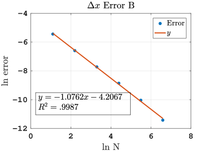
Figure 3.1: The values of (3.16) for $i=1,\ \ldots,\ 6$ depicted together with the line $y=-1.0762x-4.2067$, which was fit to the values of (3.16) with an $R^{2}$ coefficient of $R^{2}=.9987$. Parameter values of $\mathrm{Da}=66.42$, $K=1$, $l_{\mathrm{s}}=10^{-3}$, and $\epsilon=1$ were used.

4 Results and Discussion

The results of our numerical simulations are depicted in Figure 4.1. Upon inspection one immediately notices the presence of a depletion region in the center of the biochemical gate for small $t$. As time progresses, the depletion regions narrows and becomes more shallow as the rate of bound ligand production near the boundary decreases. The bound ligand concentration continues to become more spatially uniform until a chemical equilibrium is achieved, resulting in a balance between association and dissociation.

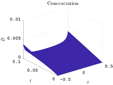
(a) Space-time curve of $B(x,t)$ for $t$ in the interval ${[}0,.1{]}$

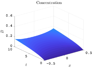
(b) Space-time curve of $B(x,t)$ for $t$ in the interval ${[}0,10{]}$.

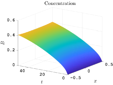
(c) Space-time curve of $B(x,t)$ for $t$ in the interval ${[}0,50{]}$.

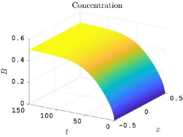
(d) Space-time curve of $B(x,t)$ for $t$ in the interval ${[}0,150{]}$.

Figure 4.1: Method of lines approximation to the solution of (2.33) during different time intervals. Parameter values of $\mathrm{Da}=66.42$, $K=1$, $l_{\mathrm{s}}=10^{-3}$, and $\epsilon=2/5$ were used.

Mathematically, the depletion region results from the singular convolution kernal

$$\tanh^{-1}(\mathrm{e}^{-|(x-\nu)|\pi l_{\mathrm{s}}/(2\epsilon)})$$ (4.1)

and the finite limits of integration. In Figure 4.2 the convolution kernel has been depicted, centered at both $x=0$ and $x=-1/2$. When the convolution kernel is centered at $x=0$ it acts as a two-sided influence function. The singularity at $x=0$ reflects the high likelihood that a ligand molecule directly above the origin will diffuse to the surface and bind with an available receptor site there; however, in the unstirred layer ligand molecules diffusing into the surface bind with neighboring receptor sites. Figure 4.2 reveals the likelihood of binding with a neighboring receptor site decays with the distance away from the source, although it is never zero since $\tanh^{-1}({\mathrm{e}^{-|x-\nu|\pi l_{\mathrm{s}}}/(2\epsilon)})$ is supported everywhere on the real line, and in particular everywhere on $[-1/2,1/2]$. Conversely, when the kernel is centered at $x=-1/2$ Figure 4.2 shows that it acts as a one-sided influence function. The finite limits of integration in (2.33a) imply that the convolution kernel influences the bound ligand concentration the most at $x=-1/2$, and has a monotonically decreasing influence progressing from $x=-1/2$ to $x=1/2$. Thus the finite limits of integration encode the reflective boundary conditions. To the right of $x=-1/2$ ligand molecules spread out and diffuse into the surface, while to the left they are merely reflected.

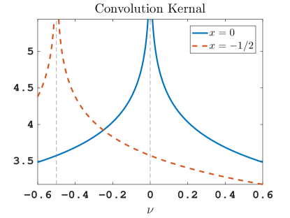
Figure 4.2: The convolution kernal $\tanh^{-1}(\mathrm{e}^{-|x-\nu|\pi l_{\mathrm{s}}/(2\epsilon)})$ centered at $x=0$ (solid line), and at $x=-1/2$ (dotted line). Parameter values of $l_{\mathrm{s}}=10^{-3}$ and $\epsilon=2/5$ were used.

The average concentration across the biochemical gate

$$\overline{B}(t)=\int_{-1/2}^{1/2}B(x,t)\ \mathrm{d}x$$ (4.2)

is shown in Figure 4.3a for three values of $\widetilde{k}_{\mathrm{a}}$. This quantity is proportional to the electrostatic potential applied to the biochemical gate, and thereby the electric current across the semi-conducting channel, allowing direct comparison to measurements. Increasing the association rate constant results in a larger Damköhler number. This reflects the enhanced rate of reaction relative to transport, and corresponds to wider and deeper depletion regions that impede current flow near the boundaries of the biochemical gate before the rest of the semiconductor channel. This is a remarkable result that is not directly observable experimentally, and provides physical insight into the origin of the signal measured with a FET. Finally, the transient phase of the signal grows with the association rate constant, owing to both decreasing the equilibrium dissociation rate constant and increasing the rate of reaction relative to diffusion.

Increasing the ligand concentration $\widetilde{C}_{\mathrm{u}}$ increases the average concentration at the biochemical gate, resulting in higher FET conductance. From Figure 4.3b it is seen that the equilibrium value of $\overline{B}$ increases with the ligand concentration $\widetilde{C}_{\mathrm{u}}$, as expected since the ligand concentration and equilibrium dissociation rate constant are inversely proportional. These considerations are clearly of fundamental importance for parameter estimation.

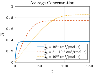
(a) The average concentration has been depicted for $\widetilde{k}_{\mathrm{a}}=10^{11},\ 5\times 10^{11}$, and $10^{12}\ \mathrm{cm}^{3}/(\mathrm{mol}\cdot\mathrm{s})$. This corresponded to $\mathrm{Da}=6.64,\ 33.21,$ and $\ 66.42$; and $K=1.67,\ 0.33,$ and $0.17$. In addition parameter values of $l_{\mathrm{s}}=10^{-3}$, and $\epsilon=2/5$ were used.

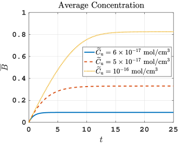
(b) The average concentration has been depicted for $\widetilde{C}_{\mathrm{u}}=10^{-17},\ 5\times 10^{-17}$, and $10^{-16}\ \mathrm{mol}/\mathrm{cm}^{3}$. This corresponded to $K=10,\ 2,$ and $0.2$. In addition parameter values of $\mathrm{Da}=6.6420,\ l_{\mathrm{s}}=10^{-3}$, and $\epsilon=2/5$ were used.

Figure 4.3: The average concentration (4.2) for different values of $\widetilde{k}_{\mathrm{a}}$ and $\widetilde{C}_{\mathrm{u}}$.

5 Conclusions

The ability to tailor therapies to individuals or specific subsets of a population could transform medicine. However, widespread use of personalized therapeutics has yet to be adopted due to our inability to quickly and routinely measure biomarkers. Not only do FETs exhibit high charge sensitivity and provide direct signal transduction, they also provide label-free measurements at physiological concentrations. As such, FETs are an incredibly promising tool for biomarker measurement. Although an accurate dynamical model for receptor-ligand dynamics is necessary for maximizing the sensitivity of these instruments, all previous modeling efforts have been devoted to the study of steady-state sensor physics. Herein, a time-dependent model for receptor ligand dynamics has been presented for the first time.

This model takes the form of a diffusion equation, coupled to an equation describing reaction on the biochemical gate. Analysis of this set of nonlinear equations is complicated by the presence of multiple disparate time and length scales: ligand molecules must diffuse a distance on the centimeters to arrive at the reacting surface, which is on the order of micrometers. Furthermore, diffusion is a very slow process while the reactions of interest proceed very quickly. Nevertheless, by using the appropriate characteristic time and length scales one is able to reduce this model to a quasi-steady transport equation for the unbound ligand concentration $C$, coupled to an equation describing the evolution of the bound ligand concentration $B$. Employing the residue theorem allows one to further reduce this set of equations to a single nonlinear IDE in terms of the reacting species concentration. Despite the presence of a singular convolution kernel, this equation has been solved to first-order accuracy without the need to resort to specialized quadrature techniques to evaluate (3.5). Results of our numerical simulations reveal the presence of a depletion region in the center of the biochemical gate, which influences the current signal by non-uniformly altering the surface-potential of the semiconductor channel.

In addition to providing a time-dependent model for estimating binding affinities, the present model could be coupled to a model for semiconductor physics to refine theoretical predictions and serve as a basis for sensor optimization. The latter may be a subject of future investigation. Additionally, it is of interest to study receptor-ligand dynamics in FETs under a different experimental conditions; i.e. a sealed experiment wherein a drop of ligand molecules is injected at an instance of time. Extending the present model to higher geometries is also of interest.

References

- [1] D. K. Armani, T. J. Kippenberg, S. M. Spillane, and K.J. Vahala. Ultra-high-Q toroid microcavity on a chip. Letters to Nature, 421(6926):925, 2003.
- [2] B. B. K., Y.-L. Zheng, V. Shukla, N. D. Amin, P. Grant, and H. C. Pant. TFP5, a peptide derived from P35, a CDK5 neuronal activator, rescues cortical neurons from glucose toxicity. Journal of Alzheimer’s Disease, 39(4):899–909, 2014.
- [3] S. Baumgartner, M. Vasicek, A. Bulyha, N. Tassotti, and C. Heitzinger. Analysis of field-effect biosensors using self-consistent 3D drift-diffusion and Monte-Carlo simulations. Procedia Engineering, 25:407–410, 2011.
- [4] R. W. Boyd and J. E. Heebner. Sensitive disk resonator photonic biosensor. Applied Optics, 40(31):5742–5747, 2001.
- [5] A. Cardone, H. Pant, and S. A. Hassan. Specific and non-specific protein association in solution: computation of solvent effects and prediction of first-encounter modes for efficient configurational bias monte carlo simulations. The Journal of Physical Chemistry B, 117(41):12360–12374, 2013.
- [6] Y. Cui, Q. Wei, H. Park, and C. M. Lieber. Nanowire nanosensors for highly sensitive and selective detection of biological and chemical species. Science, 293(5533):1289–1292, 2001.
- [7] R. Dhavan and L.-H. Tsai. A decade of cdk5. Nature reviews. Molecular Cell Biology, 2(10):749, 2001.
- [8] P. K. Drain, L. Gounder, F. Sahid, and M.-Y. Moosa. Rapid urine LAM testing improves diagnosis of expectorated smear-negative pulmonary tuberculosis in an HIV-endemic region. Scientific reports, 6:19992, 2016.
- [9] K. Fosgerau and T. Hoffmann. Peptide herapeutics: current status and future directions. Drug Discovery Today, 20(1):122–128, 2015.
- [10] C. Heitzinger, N. J. Mauser, and C. Ringhofer. Multiscale modeling of planar and nanowire field-effect biosensors. SIAM Journal on Applied Mathematics, 70(5):1634–1654, 2010.
- [11] S. Henrich, O. Salo-Ahen, B. Huang, F. F. Rippmann, G. Cruciani, and R. C. Wade. Computational approaches to identifying and characterizing protein binding sites for ligand design. Journal of Molecular Recognition, 23(2):209–219, 2010.
- [12] B. Ilic, H. G. Craighead, S. Krylov, W. Senaratne, C. Ober, and P. Neuzil. Attogram detection using nanoelectromechanical oscillators. Journal of Applied Physics, 95(7):3694–3703, 2004.
- [13] D. Johannsmann and G. Brenner. Frequency shifts of a quartz crystal microbalance calculated with the frequency-domain lattice–boltzmann method: application to coupled liquid mass. Analytical chemistry, 87(14):7476–7484, 2015.
- [14] W. Knoll. Interfaces and thin films as seen by bound electromagnetic waves. Annual Review of Physical Chemistry, 49(1):569–638, 1998.
- [15] D. Landheer, G. Aers, W. R. McKinnon, M. J. Deen, and J. C. Ranuarez. Model for the field effect from layers of biological macromolecules on the gates of metal-oxide-semiconductor transistors. Journal of Applied Physics, 98(4):044701, 2005.
- [16] S. D. Lawn and A. Gupta-Wright. Detection of lipoarabinomannan (LAM) in urine is indicative of disseminated tb with renal involvement in patients living with HIV and advanced immunodeficiency: evidence and implications. Transactions of the Royal Society of Tropical Medicine and Hygiene, 110(3):180–185, 2016.
- [17] P. Mohanty, Y. Chen, X. Wang, M. K. Hong, C. L. Rosenberg, D. T. Weaver, and S. Erramilli. Field Effect Transistor Nanosensor for Breast Cancer Diagnostics. ArXiv e-prints, 2014.
- [18] A. K. Naik, M. S. Hanay, W. K. Hiebert, X. L. Feng, and M. L. Roukes. Towards single-molecule nanomechanical mass spectrometry. Nature Nanotechnology, 4(7):445–450, 2009.
- [19] F. Pouthas, C. Gentil, D. Côte, and U. Bockelmann. DNA detection on transistor arrays following mutation-specific enzymatic amplification. Applied Physics Letters, 84(9):1594–1596, 2004.
- [20] M. Rodahl, F. Höök, A. Krozer, P. Brzezinski, and B. Kasemo. Quartz crystal microbalance setup for frequency and Q-factor measurements in gaseous and liquid environments. Review of Scientific Instruments, 66(7):3924–3930, 1995.
- [21] J. Su. Label-free single exosome detection using frequency-locked microtoroid optical resonators. ACS Photonics, 2(9):1241–1245, 2015.
- [22] G. Tulzer, S. Baumgartner, E. Brunet, G. C. Mutinati, S. Steinhauer, A. Köck, P. E. Barbano, and C. Heitzinger. Kinetic parameter estimation and fluctuation analysis of co at sno2 single nanowires. Nanotechnology, 24(31):315501, 2013.
- [23] G. Walsh. Biopharmaceutical benchmarks 2014. Nature Biotechnology, 32(10):992–1000, 2014.
- [24] S. Wang, X. Shan, U. Patel, X. Huang, J. Lu, J. Li, and N. Tao. Label-free imaging, detection, and mass measurement of single viruses by surface plasmon resonance. Proceedings of the National Academy of Sciences, 107(37):16028–16032, 2010.
- [25] W. U. Wang, C. Chen, K.-H. Lin, Y. Fang, and C. M. Lieber. Label-free detection of small-molecule–protein interactions by using nanowire nanosensors. Proceedings of the National Academy of Sciences of the United States of America, 102(9):3208–3212, 2005.