Morphing Continuum Theory for Turbulence:
Theory, Computation and Visualization

Abstract

A high order morphing continuum theory (MCT) is introduced to model highly compressible turbulence. The theory is formulated under the rigorous framework of rational continuum mechanics. A set of linear constitutive equations and balance laws are deduced and presented from the Coleman-Noll procedure and Onsager’s reciprocal relations. The governing equations are then arranged in conservation form and solved through the finite volume method with a second order Lax-Friedrichs scheme for shock preservation. A numerical example of transonic flow over a three-dimensional bump is presented using MCT and the finite volume method. The comparison shows that MCT-based DNS provides a better prediction than NS-based DNS with less than 10% of the mesh number when compared with experiments. A MCT-based and frame-indifferent Q-criterion is also derived to show the coherent eddy structure of the downstream turbulence in the numerical example. It should be emphasized that unlike the NS-based G-criterion, the MCT-based Q-criterion is objective without the limitation of Galilean-invariance.

I Introduction

Navier-Stokes (NS) equations have been extensively used to study flow physics for several decades. Other than deriving the balance laws from the Reynolds Transport Theorem and the three-dimensional Leibniz Theorem common seen in undergraduate textbooks Batchelor (1967), these laws can also be derived independently from rational continuum mechanics (RCM) Eringen (1971, 1980); Truesdell and Rajapogal (1999); Truesdell (1966) or Boltzmann’s kinetic theory Boltzmann (1964); Huang (1963); Ferziger and Kaper (1972). or Classical Irreversible Thermodynamics Gyarmati (1961a, b); Li (1967); Coleman and Noll (1963); Chen (2013); Müller and Ruggeri (1991). This procedure pairs independent variables and response functions as thermodynamic forces and fluxes, i.e. a thermodynamic conjugate Gyarmati (1961a, b); Li (1967). The Helmholtz free energy is expanded with thermodynamic forces and the thermodynamic flux is then found as the derivative of the Helmholtz free energy with respect to the corresponding thermodynamic force. The derivation process for linear constitutive equations was understood as the Onsager–Casimir relations Onsager (1931a, b); De Groot and Mazur (1962). Nevertheless, though the framework is mathematically rigorous and theoretically sounding, understanding the physics represented by the material constants in those equations heavily relies on experimental observation and measurements.

At the same time, kinetic theory approximates the gas atoms as points and model the interaction as collisions. Boltzmann derived a distribution function for equilibrium states with H-theorem and introduced a conservation equation with a collision integral Huang (1963); Boltzmann (1964). With the proper definitions for kinetic variables, e.g. mass, linear momentum and energy, the conservations equations leads to the balance laws Ferziger and Kaper (1972). However, systems are rarely in equilibrium. As a result, the distribution function varies with the interactions between gas atoms through the collision integral. If the distribution is assumed to linearly deviate from the Boltzmann distribution, the balance law of linear momentum leads to the celebrated NS equations Huang (1963). Since kinetic theory is a physics-based approach, the physical meanings of material constants are explained through the inter-particle collisions. For example, Maxwell showed that the viscosity is independent of the density for a given temperature through kinetic theory and later verified this fact with experiments Huang (1963). For dilute gases, kinetic theory also shows a linear relation for the ratio of thermal conductivity to the product of the viscosity and specific heat. Though kinetic theory provides a detailed insights for the governing equations and material constants, Truesdell raised a concern that all equations derived from kinetic theory only contain a subset of those from rational continuum theory and claimed the validity of the continuum equations are beyond rarefied gases Truesdell (1984).

Regardless of different theoretical origins, NS equations have been the core of the fluid dynamics research ranging from turbulence to vortex-dominated flows for decades. Nevertheless, assumptions made in NS equations should always be kept in mind. Rational continuum mechanics assumes a continuum homogenizing volumeless points. On the other hand, kinetic theory approximates continuous medium populated with monoatomic gases. This approximation results in a compromise of relying on an orbital angular velocity, i.e. vorticity, to describe rotational motions in fluids. In other words, vorticity or vorticity-based methods have been employed to describe the rotational eddies in turbulent flows, coherent vorticies in dynamic stall or body-vortex interaction in biomimetics. However, vorticity-based approaches are only Galilean invariant and present inconsistent results for vortex visualization from Q-criterion and $\lambda_{2}$ method in rotating flows Haller (2005). Therefore, Speziale and Haller have been emphasizing the importance of objectivity or frame-indifference for vortex descriptions and turbulence models Speziale (1979, 1987); Speziale et al. (1991); Haller (2005). Further, revealing the detailed eddy structures with vorticity-based method requires extremely fine mesh for numerical differentiation. These arbitrarily fine meshes cause heavy computational burden and make numerical simulation impractical even with the best computational power available today Zhong and Wang (2012).

The Cosserat Brothers initiated the concept of a morphing continuum theory (MCT), i.e. a continuous space containing inner structures Cosserat and Cosserat (1909). Later, Eringen formulated a class of morphing continuum allowing rotation at subscale under the framework of rational continuum mechanics and classical irreversible thermodynamics Eringen (1999). Independently, Grad introduced a concept of a continuum with arbitrary number of internal degrees of freedom and proposed a first order differential equation for spins Grad (1952). De Groot and Mazur extended Grad’s formulation and proposed a balance law for the internal spins De Groot and Mazur (1962). Snider and Lewchuk later completed Grad’s formulations with irreversible thermodynamics Snider and Lewchuk (1967). The theoretical studies independently initiated by Eringen and Grad were found to be identical.

Similar to the works done for NS equations with statistical mechanics and kinetic theory, She and Sather relied on the Chapman-Enskog method to derive a kinetic theory for molecules with arbitrary internal degrees of freedom She and Sather (1967). Brau evaluated several different collision processes under She and Sather’s formulations Brau (1967). Curtiss later integrated these studies and officially introduced kinetic theory for molecular gases Curtiss (1992).

To the author’s limited knowledge, the detailed comparison between irreversible thermodynamics/rational continuum mechanics and statistical kinetic theory was first presented in the book, Rational Extended Thermodynamics, by Müller and RuggeriMüller and Ruggeri (1991). Rational Extended Thermodynamics has been used to derive governing equations for shock wave structure, light scattering, radiation, relativistic mechanics, phonons and metal electrons Müller and Ruggeri (1991). For monoatomic gases, the phenomenological equations derived from kinetic theory are found to be identical to those from thermodynamics of irreversible process. Motivated by these early studies, Chen recently proved that the inviscid version of the MCT governing equations from rational continuum mechanics/irreversible thermodynamics are identical to the balance laws at equilibrium from Curtiss’ molecular kinetic theory Chen (2016, ress). This study unifies both formulations in kinetic theory and rational continuum mechanics for fluid system with internal spins, and derives the Boltzmann-Curtiss distribution from a quantum statistics perspective Chen (2016, ress).

Since its introduction , MCT has been used to study the flow physics with significant internal spins, eg. turbulence Kirwan and Newman (1969); Liu (1970); Eringen and Chang (1970); Peddieson (1972); Ahmadi (1975, 1981); Brutyan and Krapivsky (1992). Ahmadi extended the work of Liu Liu (1970) to construct a statistical theory for turbulence via a functional approach Ahmadi (1981). Peddieson was the first one proposing MCT dimensionless parameters to characterize the wall shear layers in the boundary layer turbulence Peddieson (1972). More recently, Mehrabian and Atefi compared the analytical solution of plane Poiseulle flow in MCT with the experimental velocity profiles, both laminar and turbulent Mehrabian and Atefi (2008). Alizadeth et. al. reformulated MCT and studied the turbulent plane Couette flow with slip. The simulation results agree extremely well with the experiments Alizadeth et al. (2011). However, all the aforementioned studies are limited in the analytical solutions for incompressible flows. More recently, researchers have been focusing on developing numerical methods for MCT in both incompressible and compressible flows Chen et al. (2010, 2012); Crnjavic-Zic and Mujakovic (2016); Drazic et al. (2017).

With the rapid developments on the numerical solvers, a series of studies were published on incompressible and compressible turbulence and their statistical characteristics Wonnell and Chen (2016, 2017a); Cheikh and Chen (2017); Wonnell and Chen (2017b). Cheikh and Chen validated that MCT is capable of predicting the velocity profile over a compression ramp in a supersonic turbulence Cheikh and Chen (2017). However, MCT is still relatively new to turbulence community. Tools for turbulence analysis and visualization are at their infancy. Therefore, this study will summarize the derivation of MCT, its connection to turbulence, and an objective tool for visualizing coherent eddy structures. The derivation of MCT is briefly reviewed in Section II. The MCT governing equations will be rearranged in the conservation forms for numerical methods implementations, e.g. finite difference method, finite volume method and others, in Section III. In Section IV, a numerical example of a transonic flow over a three-dimensional bump will be briefly presented. An objective Q-critirion with MCT will be derived and discussed in details for eddy and vortex visualizations. Section V concludes the highlights and remarks of this study.

II Morphing Continuum Theory

A morphing continuum is a collection of continuously distributed, oriented, finite-size subscale structures that allows rotations. A material point $P$ in the reference frame is identified by a position and three directors attached to the material point.

The motion, at time $t$, carries the finite-size subscale structure to a spatial point and rotates the three directors to a new orientation. Thus, such a motion can be understood as the motion of a liquid molecule or an eddy approximated as a rigid body. MCT possesses not only translational velocity, but also self-spinning gyration on its own axis. These motions and their inverse motions for the morphing continuum can be described as Eringen (1999)

$$x_{k} =x_{k}(X_{K},t)\quad X_{K} =X_{K}(x_{k},t)$$

$$\xi_{k} =\chi_{kK}(X_{K},t)\Xi_{K}\quad \Xi_{K} =\bar{\chi}_{Kk}\xi_{k}$$ (1)

$$K =1,2,3\quad k =1,2,3$$

and

$$\chi_{kK}\chi_{lK}=\delta_{kl}\qquad\bar{\chi}_{Kk}\bar{\chi}_{Lk}=\delta_{KL}.$$ (2)

where the lowercase index is for the Eulerian coordinate while the uppercase index for the Lagrangian coordinate.

It is straightforward to prove that

$$\chi_{kK}=\bar{\chi}_{Kk}.$$ (3)

Consequently, the righthand side of eq. 2 becomes

$$\chi_{kK}\chi_{kL}=\delta_{KL}.$$ (4)

Here and throughout, an index followed by a comma denotes a partial derivative, e.g.,

$$x_{k,K}=\frac{\partial x_{k}}{\partial X_{K}}\qquad\mbox{and}\qquad X_{K,k}=\frac{\partial X_{K}}{\partial x_{k}}.$$ (5)

For fluid flow, deformation-rate tensors are used to characterize the viscous resistance. Deformation-rate tensors may be deduced by calculating the material time derivative of the spatial deformation tensors. For a morphing continuum, two objective deformation-rate tensors can be derived as

$$a_{kl}=v_{l,k}+e_{lkm}\omega_{m}\qquad\mbox{and}\qquad b_{kl}=\omega_{k,l},$$ (6)

where $v_{k}$ is the velocity vector and $\omega_{k}$ is the self-spinning gyration vector. The fluid or flow inner structure possesses two types of motion, translational velocity ($v_{k}$), found by solving the MCT linear momentum equation, and spinning gyration ($\omega_{k}$) found by solving the MCT angular momentum equation. In the classical Navier-Stokes equations, the translational velocity can be directly solved from the balance law of linear momentum. To investigate the effect of the rotational motion of the subscale structure, one must use the velocity field and take the angular velocity to be one-half of the vorticity i.e., $\frac{1}{2}e_{ijk}v_{j,i}$. This approximation in the Navier-Stokes equations limits not only predicting the flow physics involving spinning, but also fails to represent the interaction between translation and spinning Snider and Lewchuk (1967). In addition, highly refined meshes are also needed in order to obtain high resolution vorticity fields. This arbitrary mesh requirement makes numerical simulations in realistic environments impractical Zhong and Wang (2012). On the other hand, MCT provides both the self-spinning motion and the relative rotation, e.g. vorticity. The arbitrarily fine meshes are no longer required since part of the information on rotational motions can be directly obtained from self-spinning gyration.

II.1 Balance Laws

Thermodynamic balance laws for morphing continuum theory include (1) mass; (2) linear momentum; (3) angular momentum; (4) energy; and (5) the Clausius-Duhem inequality. All five can be expressed as follows:

Conservation of mass

$$\frac{\partial\rho}{\partial t}+(\rho v_{i})_{,i}=0$$ (7)

Balance of linear momentum

$$t_{lk,l}+\rho(f_{k}-\dot{v}_{k})=0$$ (8)

Balance of angular momentum

$$m_{lk,l}+e_{ijk}t_{ij}+\rho i_{km}(l_{m}-\dot{\omega}_{m})=0$$ (9)

Balance of energy

$$\rho\dot{e}-t_{kl}a_{kl}-m_{kl}b_{lk}+q_{k,k}=0$$ (10)

Clausius-Duhem inequality

$$\rho(\dot{\psi}+\eta\dot{\theta})+t_{kl}a_{kl}+m_{kl}b_{lk}-\frac{q_{k}}{\theta}\theta_{,k}\geq 0$$ (11)

where $\rho$ is mass density, $i_{km}$ the microinertia for the shape of the microstructure, $f_{k}$ the body force density, $l_{m}$ the body moment density, $e$ the internal energy density, $\eta$ the entropy density, $\psi=e-\theta\eta$ the Helmholtz free energy, $t_{lk}$ the Cauchy stress, $m_{lk}$ the moment of stress, and $q_{k}$ the heat flux. It is worthwhile to mention that $t_{lk}$, $m_{lk}$ and $q_{k}$ are the constitutive equations for the morphing continuum theory and can be derived from the Clausius-Duhem inequality (see eq. 11) through the Coleman-Noll procedure Chen et al. (2011); Coleman and Noll (1963).

The concept of subscale inertia, $i_{km}\equiv{\int\rho^{\prime}\xi_{k}\xi_{m}dv^{\prime}}/{\int\rho^{\prime}dv^{\prime}}\equiv\langle\xi_{k}\xi_{m}\rangle$, is similar to the moment of inertia in rigid body rotation and measures the resistance of the subscale structure to changes to its rotation. It can be further expressed as

$$j_{km}=i_{pp}\delta_{km}-i_{km}\qquad\mbox{where}\qquad j\equiv\frac{1}{3}j_{pp}.$$ (12)

The volume $v^{\prime}$ refers to the volume of the subscale structure. If the subscale structure is assumed to be a rigid sphere with a radius $d$ and a constant density $\rho$, the subscale inertia can be computed as $j=\frac{2}{5}d^{2}$. This result shows the subscale inertia for a sphere is the moment of inertia of a sphere divided by its mass. The experimental data of Lagrangian velocities of a trace particle can be used to determine the geometry of the subscale structure Chen et al. (2011); Mordant et al. (2001). The new degrees of freedom, gyration, in MCT can also be directly compared with the direct experimental measurement of vorticity Ryabtsev et al. (2016).

II.2 Constitutive Equations

There are multiple different definitions for fluids, including (1) fluids do not have a preferred shape Batchelor (1967), and (2), fluids cannot withstand shearing forces, however small, without sustained motion Panton (2013). Nevertheless, all these definitions describe the physics of fluid flow, and yet provide little help in mathematically formulating a continuum theory for fluids. In rational continuum mechanics, Eringen formally defined fluids by saying that “a body is called fluid if every configuration of the body leaving density unchanged can be taken as the reference configuration”Eringen (1980). This definition implies $x_{k,K}\rightarrow\delta_{kK}$ and $\chi_{kK}\rightarrow\delta_{kK}$ where $\delta_{kK}$ is the shifter, the directional cosine between the current configuration and reference configuration.

Objectivity is followed throughout the derivation of constitutive equations. The axiom of objectivity, or frame-indifference, states that the constitutive equations must be form-invariant with respect to rigid body motions of the spatial frame of reference Eringen (1971, 1980); Truesdell (1966); Truesdell and Rajapogal (1999).

The state of fluids in morphing continuum theory is expressed by the characterization of the response functions $\mathbf{Y}=\{\psi,\eta,t_{kl},m_{kl},q_{k}\}$ as functions of a set of independent variables $\mathbf{Z}=\{\rho^{-1},\theta,\theta_{,k},a_{kl},b_{kl}\}$. At the outset the constitutive relations are written as $\mathbf{Y}=\mathbf{Y}(\mathbf{Z})$ Eringen (2001).

The Clausius-Duhem inequality of eq. 11, also known as the thermodynamic second law, is a statement concerning the irreversibility of natural processes, especially when energy dissipation is involved. Feynman et. al. stated “so we see that a substance must be limited in a certain way; one cannot make up anything he wants; … This [entropy] principle, this limitation, is the only rule that comes out of thermodynamics” Feynman et al. (1970). After the Coleman-Noll procedure, i.e., combining the inequality with the response function and the independent variables, eq. 11 reduces to

$$t_{kl}^{d}a_{kl}+m_{kl}b_{lk}-\frac{q_{k}\theta_{,k}}{\theta}\geq 0.$$ (13)

The current formulation relying on the Coleman-Noll procedure only provides local entropy increase and the conditions for first order weakly nonlocal state.

In eq. 13, there are three pairs of thermodynamic conjugates, ($t_{kl}^{d}$, $a_{kl}$), ($m_{kl}$, $b_{lk}$), and ($\frac{q_{k}}{\theta}$,$\theta_{,k}$) that contribute to the irreversibility of the material. A set of the thermodynamic fluxes $\mathbf{J}$ is defined as $\mathbf{J}=\{t_{kl}^{d},m_{kl},\frac{q_{k}}{\theta}\}$ and are functions of a set of the thermodynamic forces ($\mathbf{Z}^{D}$) and other independent variables ($\mathbf{Z}^{R}$), $\mathbf{Z}=\{\mathbf{Z}^{R};\mathbf{Z}^{D}\}=\{\rho^{-1},\theta;a_{kl},b_{lk},\theta_{,k}\}$. With these sets of thermodynamic fluxes and thermodynamic forces, the Clausius-Duhem inequality can be rewritten as

$$\mathbf{J}(\mathbf{Z}^{R};\mathbf{Z}^{D})\cdot\mathbf{Z}^{D}\geq 0.$$ (14)

Onsager and others proposed that the thermodynamic fluxes can be obtained by the general dissipative function Chen (2013); Edelen (1972); Onsager (1931a, b); Gyarmati (1961a, b); Li (1967)

$$\mathbf{J}=\frac{\partial\Psi(\mathbf{Z}^{R},\mathbf{Z}^{D})}{\partial\mathbf{Z}^{D}}+\mathbf{U},$$ (15)

where the vector-valued function $\mathbf{U}$ is the constitutive residual with $\mathbf{Z}^{D}\cdot\mathbf{U}=0$. This result indicates that $\mathbf{U}$ does not contribute to the dissipative or entropy production. For simplicity, one can further set $\mathbf{U}=0$.

To determine thermodynamic fluxes for a fluid using the derivative of $\Psi$ with respect to the thermodynamic forces $\mathbf{Z}^{D}$, $\Psi$ needs to be invariant under superimposed rigid body motion, i.e., the dissipative function $\Psi$ must satisfy the axiom of objectivity Chen (2013). Hence, $\Psi$ is an isotropic function of scalar and can be expressed by Wang’s representation theorem Wang (1969, 1970) as

$$\Psi\{\mathbf{Z}^{R},\mathbf{Z}^{D}\}=\Psi\{I_{1},I_{2},I_{3},...,I_{n}\}$$

and

$$\mathbf{J}=\frac{\partial\Psi}{\partial\mathbf{Z}^{D}}=\sum_{i=1}^{n}\frac{\partial\Psi}{\partial I_{i}}\frac{\partial I_{i}}{\partial\mathbf{Z}^{D}}.$$ (16)

It should be noted here that $b_{lk}$ and $m_{kl}$ are pseudo-tensors while the rest, including $\theta_{,k}$, $t_{kl}^{d}$, $q_{k}$ and $a_{kl}$ are normal tensors Chen et al. (2011). Considering the mixing of pseudo-tensors and normal tensors in $\mathbf{Z}^{R}$ and $\mathbf{Z}^{D}$ for linear constitutive equations, the set of invariants includes $I_{1}=a_{(ii)}$, $I_{2}=a_{(ij)}a_{(ji)}$, $I_{3}=b_{(ij)}b_{(ji)}$, $I_{4}=\theta_{,k}\theta_{,k}$, $I_{5}=a_{[ij]}a_{[ji]}$, $I_{6}=b_{[ij]}b_{[ji]}$, and $I_{7}=e_{ijk}b_{ij}\theta_{k}$ . Here (…) refers to the symmetric part, […] indicates the anti-symmetric part and $e_{ijk}$ is the permutation symbol. Hence, the thermodynamic fluxes can be further derived as

$$t_{kl}^{d} =t_{(kl)}^{d}+t_{[kl]}^{d}$$

$$=\frac{\partial\Psi}{\partial a_{(kl)}}+\frac{\partial\Psi}{\partial a_{[kl]}}$$

$$=\frac{\partial\Psi}{\partial I_{1}}\delta_{kl}+\frac{\partial\Psi}{\partial I_{2}}a_{(kl)}+\frac{\partial\Psi}{\partial I_{5}}a_{[kl]}$$

$$=\lambda a_{mm}\delta_{kl}+2\mu a_{(kl)}+\kappa(a_{(kl)}+a_{[kl]})$$

$$m_{kl} =m_{(kl)}+m_{[kl]}$$

$$=\frac{\partial\Psi}{\partial b_{(kl)}}+\frac{\partial\Psi}{\partial b_{[kl]}}$$

$$=\frac{\partial\Psi}{\partial I_{3}}b_{(kl)}+\frac{\partial\Psi}{\partial I_{6}}b_{[kl]}+\frac{\partial\Psi}{\partial I_{7}}e_{klm}\theta_{,m}$$

$$=\alpha b_{mm}\delta_{kl}+\frac{1}{2}(\beta+\gamma)b_{(kl)}+\frac{1}{2}(\beta-\gamma)b_{[kl]}+\frac{\alpha_{T}}{\theta}e_{klm}\theta_{,m}$$

$$q_{k} =\frac{\partial\Psi}{\partial\theta_{,k}}$$

$$=\frac{\partial\Psi}{\partial I_{4}}\theta_{,k}+\frac{\partial\Psi}{\partial I_{7}}e_{ijk}b_{ij}$$

$$=K\theta_{,m}+\frac{\alpha_{T}}{\theta}e_{klm}b_{[kl]}$$ (17)

These equations can also be put into matrix form as

$$\quad\begin{bmatrix}t_{(kl)}^{d}\\ t_{[kl]}^{d}\\ m_{(kl)}\\ m_{[kl]}\\ q_{k}\end{bmatrix}$$ (18)

$$=\begin{bmatrix}\lambda\delta_{kl}+2\mu+\kappa&0&0&0&0\\ 0&\kappa&0&0&0\\ 0&0&\alpha\delta_{kl}+\frac{1}{2}(\beta+\gamma)&0&0\\ 0&0&0&\frac{1}{2}(\beta-\gamma)&\frac{\alpha_{T}e_{klm}}{\theta}\\ 0&0&0&\frac{\alpha_{T}e_{klm}}{\theta}&K\end{bmatrix}$$

$$\begin{bmatrix}a_{(kl)}\\ a_{[kl]}\\ b_{(kl)}\\ b_{[kl]}\\ \theta_{,m}\end{bmatrix}$$

$$=\begin{bmatrix}\lambda\delta_{kl}+2\mu+\kappa&0&0&0&0\\ 0&\kappa&0&0&0\\ 0&0&\alpha\delta_{kl}+\frac{1}{2}(\beta+\gamma)&0&0\\ 0&0&0&\frac{1}{2}(\beta-\gamma)&\frac{\alpha_{T}e_{klm}}{\theta}\\ 0&0&0&\frac{\alpha_{T}e_{klm}}{\theta}&K\end{bmatrix}$$

$$\begin{bmatrix}\frac{1}{2}(v_{k,l}+v_{l,k})\\ \frac{1}{2}(v_{l,k}-v_{k,l}+2e_{lkm}\omega_{m})\\ \frac{1}{2}(\omega_{k,l}+\omega_{l,k})\\ \frac{1}{2}(\omega_{k,l}-\omega_{l,k})\\ \theta_{,m}\end{bmatrix}.$$ (19)

Notice the symmetry of this thermodynamic matrix. Equations 19 connect the thermodynamic fluxes and the thermodynamic forces, and can be referred to as Onsager’s reciprocal relations derived in 1931 Onsager (1931a, b) leading to his Nobel Prize in Chemistry in 1968. It should be noted that the reciprocity is the condition for the existence of the dissipative potential $\check{S}$ilhavý (1997); Berezovski and Van (2017). With further algebraic manipulation, the linear constitutive equations for the morphing continuum are

$$t_{lk} =-p\delta_{kl}+\lambda v_{m,m}\delta_{kl}+\mu(v_{k,l}+v_{l,k})+\kappa(v_{k,l}+e_{klm}\omega_{m})$$

$$m_{lk} =\frac{\alpha_{T}}{\theta}e_{lkm}\theta_{,m}+\alpha\omega_{m,m}\delta_{kl}+\beta\omega_{l,k}+\gamma\omega_{k,l}$$

$$q_{k} =\frac{\alpha_{T}}{\theta}e_{lkm}\omega_{k,l}+K\theta_{,m}$$ (20)

where $\mu$ is the viscosity, $\lambda$ is the secondary viscosity, $\kappa$ is the subscale viscosity, $\gamma$ is the subscale diffusivity and $\alpha$ & $\beta$ are related to the compressibility of the subscale structure. Inserting eq. 20 to all the balance laws, eqs. 7-10, omitting body force and adopting a spherical subscale structure, the MCT governing equations can be rewritten as

Conservation of mass

$$\frac{\partial\rho}{\partial t}+(\rho v_{i})_{,i}=0$$ (21)

Balance of linear momentum

$$\rho(\frac{\partial v_{k}}{\partial t}+v_{i}v_{k,i})$$

$$=-p_{k}+(\lambda+\mu)v_{m,mk}+(\mu+\kappa)v_{k,ll}+\kappa e_{kij}\omega_{j,i}$$ (22)

Balance of angular momentum

$$\rho j(\frac{\partial\omega_{m}}{\partial t}+v_{i}\omega_{m,i})$$

$$=(\alpha+\beta)\omega_{m,mk}+\gamma\omega_{m,ll}+\kappa(e_{mnk}v_{k,n}-2\omega_{m})$$ (23)

Balance of energy

$$\rho(\frac{\partial e}{\partial t}+v_{i}e_{,i})$$

$$=[-p\delta_{kl}+\lambda v_{m,m}\delta_{kl}+\mu(v_{k,l}+v_{l,k})+\kappa(v_{l,k}+e_{lkm}\omega_{m})]$$

$$\qquad\qquad\qquad\qquad\qquad\qquad\qquad\qquad\qquad(v_{l,k}+e_{lkm}\omega_{m})$$

$$+(\frac{\alpha_{T}}{\theta}e_{klm}\theta_{,m}+\alpha\omega_{m,m}\delta_{kl}+\beta\omega_{k,l}+\gamma\omega_{l,k})\omega_{k,l}$$

$$+K\theta_{,mm}$$ (24)

III Numerical Methods

Equations 21 - 24 can be directly discretized and solved with the classical finite difference method Chen et al. (2010); however, in order to adopt modern numerical schemes, such as finite volume method Cheikh and Chen (2017); Patankar (1984), spectral difference method Chen et al. (2012); Liu et al. (2006a); Wang et al. (2007), spectral volume method Wang (2002); Liu et al. (2006b) and others Nishikawa and Liu (2017), the governing equations should be cast into the conservation forms. Chen et. al. formulated the conservation form for MCT as Chen et al. (2012)

$$\frac{\partial\rho}{\partial t}+\nabla\cdot(\rho\vec{v})=0$$ (25)

$$\frac{\partial\rho\vec{v}}{\partial t}+\nabla\cdot(\vec{v}\otimes\rho\vec{v})=$$

$$\quad-\nabla p+(\lambda+\mu)\nabla\nabla\cdot\vec{v}+(\mu+\kappa)\nabla^{2}\vec{v}+\kappa\nabla\times\vec{v}$$ (26)

$$\frac{\partial\rho j\vec{\omega}}{\partial t}+\nabla\cdot(\vec{v}\otimes\rho j\vec{\omega})=$$

$$\qquad\qquad(\alpha+\beta)\nabla\nabla\cdot\vec{\omega}+\gamma\nabla^{2}\vec{\omega}+\kappa(\nabla\times\vec{v}-2\vec{\omega})$$ (27)

$$\frac{\partial\rho E}{\partial t}+\nabla\cdot(\vec{v}\rho E)=$$

$$\qquad\qquad\qquad\qquad\nabla\cdot(\mathbf{t}\cdot\vec{v})+\nabla\cdot(\mathbf{m}\cdot\vec{\omega})-\nabla\cdot\vec{q}$$ (28)

where $\mathbf{t}$ is the MCT Cauchy stress, $\mathbf{m}$ is the MCT moment stress and $\vec{q}$ is the MCT heat flux (cf. eq.20). In addition, $E$ is the MCT total energy defined as the sum of inernal energy density, translational kinetic energy density and rotational kinetic energy density as $E=e+\frac{1}{2}(\vec{v}\cdot\vec{v}+j\vec{\omega}\cdot\vec{\omega})$.

Several researchers have started focusing on numerical methods for MCT Chen et al. (2010, 2012); Drazic et al. (2017); Crnjavic-Zic and Mujakovic (2016); Mujakovic and Crnjaric-Zic (2015). More specifically, three different numerical schemes are introduced in the past few years: (1) finite difference method with second order temporal and spatial accuracy for incompressible flows Chen et al. (2010); (2) finite volume method with second order shock preserving scheme for compressible flows Cheikh and Chen (2017); and (3) high order spectral difference method for compressible flows Chen et al. (2012). In this study, the finite volume method with second order shock preserving scheme is used and summarized as follows.

The finite volume method directly implements a numerical procedure solving the conservation forms of governing equations. The general form over a control volume can be expressed as

$$\frac{\partial\Psi}{\partial t}+\nabla\cdot(\vec{v}\Psi)-\nabla\cdot(\Gamma\nabla\Psi)=S_{\Psi}$$ (29)

where $\Psi$ is any physical quantity, $\frac{\partial\Psi}{\partial t}$ is the unsteady term, $\nabla\cdot(\vec{v}\Psi)$ is the convective term, $\nabla\cdot(\Gamma\nabla\Psi)$ is the diffusion term and $S_{\Psi}$ is the source term.

The diffusion term is discretized by the central difference method and Green-Gauss theorem, i.e.

$$\int_{V}\nabla\cdot(\Gamma\nabla\Psi)dV =\oint_{\vec{A}}\Gamma\nabla\Psi\cdot d\vec{A}$$

$$\approx\sum_{f}\Gamma_{f}\vec{A}_{f}\cdot\nabla\Psi_{f}$$ (30)

where $V$ is the control volume, $\vec{A}$ is the enclosed surfaces with normal vectors for the control volume and $f$ indicates each surfaces in the control volume for calculation.

The convective term is discretized by the second order Lax-Friedrich flux splitting method by Kuganov, Noelle and Petrova (KNP) Kurganov et al. (2001), i.e.

$$\int_{V}\nabla\cdot(\vec{v}\Psi)dV =\oint_{\vec{A}}\vec{v}\Psi\cdot d\vec{A}$$

$$\approx\sum_{f}\vec{A}_{f}\cdot\vec{v}_{f}\Psi_{f}$$

$$=\sum_{f}\phi_{f}\Psi_{f}$$ (31)

and

$$\sum_{f}\phi_{f}\Psi_{f}= \sum_{f}[\alpha\phi_{f+}\Psi_{f+}$$

$$+(1-\alpha)\phi_{f-}\Psi_{f-}+\omega_{f}(\Psi_{f-}-\Psi_{f+})]$$ (32)

where $\alpha$ is calculated based on the local speed of sound, ie.

$$\Psi_{f+}=\text{max}(c_{f+}|\vec{A}_{f}|+\phi_{f+},c_{f-}|\vec{A}_{f}|+\phi_{f-},0)$$

$$\Psi_{f-}=\text{max}(c_{f+}|\vec{A}_{f}|-\phi_{f+},c_{f-}|\vec{A}_{f}|-\phi_{f-},0)$$

$$\alpha=\frac{\Psi_{f+}}{\Psi_{f+}+\Psi_{f-}}$$

$$\omega_{f}=\alpha(1-\alpha)(\Psi_{f+}+\Psi_{f-})$$ (33)

The gradient and curl term is also discretized by the second order Lax-Friedrich flux splitting method, similar to the convective terms.

$$\int_{V}\nabla\Psi dV =\oint_{\vec{A}}\Psi d\vec{A}$$

$$=\sum_{f}\vec{A}_{f}\Psi_{f}$$ (34)

where the KNP scheme further split the interpolation procedure into $f_{+}$ and $f_{-}$ direction, ie.

$$\sum_{f}\vec{A}_{f}\Psi_{f}=\sum_{f}[\alpha\vec{A}\Psi_{f+}+(1-\alpha)\vec{A}\Psi_{f-}]$$ (35)

This second order generalized Lax-Friedrich flux was implemented in the NS framework. Cheikh and Chen further demonstrated that this approach also provides a second order accuracy in space for MCT Cheikh and Chen (2017). If the discretized equations are solved in a explicit manner, the unsteady term can be marched with Runge-Kutta method of any order in temporal accuracy. In this study, a first order Euler method is chosen for convenience.

IV Numerical Example - Transonic Flows over a 3D Bump

There have been a significant amount of studies on turbulence simulation and analysis with morphing continuum theories since the 1970s Ahmadi (1975, 1981); Brutyan and Krapivsky (1992); Eringen and Chang (1970); Peddieson (1972); Kirwan and Newman (1969); Mehrabian and Atefi (2008); Wonnell and Chen (2016); Cheikh and Chen (2017); Wonnell and Chen (2017a, b); Alizadeth et al. (2011). Most of the published efforts focused on the velocity profile with analytical means. With the assistance of the introduced finite volume method with shock preserving scheme in Sect. III, a transonic flow of Ma$=0.6$ over a 3D bump is simulated and compared with experimental measurements Simpson et al. (2002) and NS-based direct numerical simulation (DNS) results Castagna et al. (2014).

IV.1 MCT Simulation Compared with DNS and Experiments

The inlet is specified with a turbulent boundary layer flow with a thickness of $\delta=39$ mm and the free stream velocity of $M_{\infty}=0.6$. The corresponding $Re_{\delta}*=500$ while $Re_{\delta}$ is 6.5 times of the $Re_{\delta}*$. The boundary layer flows over a three dimensional bump with the height of $H=78$ mm. The NS-based DNS (NS-DNS) study on this problem was reported and presented side by side with a comparable experiment in 2014 Castagna et al. (2014). A MCT-based DNS (MCT-DNS) is performed following exactly the same setup reported in the NS-DNS study for the purpose of comparison. The pressure coefficient from NS-DNS (dashline) Castagna et al. (2014), experiment (circle) Simpson et al. (2002) and MCT-DNS (solid line) Wonnell and Chen (2017b) is shown in Figure 1. It can be seen that the NS-DNS only captures one experimental data point over the bum and is unable to clearly identify the normal shock. On the other hand, MCT-DNS captures most of the experimental data points over the normal shock and agrees better with the experiment. In addition, MCT also has a better prediction than NS on the pressure coefficient downstream. It should be mentioned that the deviation between the experiment and simulation is caused by the separation point in the flow. Neither NS nor MCT was able to predict the correct separation point. This inconsistency is due to the unknown channel surface properties, such as roughness, and the fluid properties. The fluid used in the experiment was kerosene while both NS and MCT simulation focused on the equivalence of dimensionless parameters comparable with experiments.

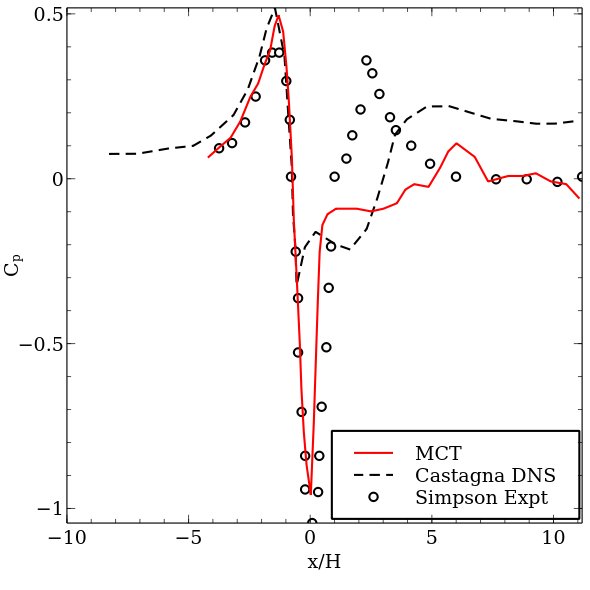
Figure 1: Pressure coefficient comparison among experiment, DNS and MCT along the centerline on the bump

The required computational resources between NS and MCT are also compared. The NS work adopts a high order finite difference method with a mesh number totaling $\sim$ 54M Castagna et al. (2014). On the other hand, MCT was solved with a second order finite volume method with a shock preserving scheme and used a mesh number of $\sim$ 4.5M. With less than 10% of the cell number required in DNS, MCT was able to have a better prediction on shock position and the pressure profile in the downstream turbulence. The multiscale nature of MCT provides a rigorous framework coupling one level of motion for macroscale translation and another one for subscale eddy rotation. Therefore, there is no need for arbitrary fine mesh in capturing the subscale motion. In MCT, most of the subscale motions are captured by the additional degrees of freedom (gyration) at subscale. Part of these results were reported in AIAA Aviation 2017 Wonnell and Chen (2017b). Unlike the classical Reynolds-Averaging Numerical Simulation (RANS) or Large Eddy Simulation (LES), MCT does not require any turbulence models. The numerical solution of MCT is acquired in the same fashion of direct numerical simulation for NS equations. The flow at subscales are resolved by the additional degrees of freedom, gyration.

With a successful prediction from MCT, it is necessary to provide a tool to visualize the classical hairpin eddy structure in turbulence. However, the classical velocity-based criteria have been criticized on the inconsistency and limitation on being only Galilean invariant Haller (2005). The multiscale MCT can be further developed into a visualization tool with objectivity (or frame-indifference) and similar physical meanings provided by the classical criteria.

IV.2 Objective Description of Vortex Visualization

Speziale devoted part of his career laying down the foundamentals of objectivity and investigated the requirment of objectivity over Galilean invariance for turbulence simulation Speziale (1979, 1987, 1989, 1998); Speziale et al. (1991). More recently, Haller showed the inconsistency of vortex identification with the classical velocity gradient-based approaches and emphasized the importance of the objectivity or frame-indifference for vortex visualization Haller (2005). The classical Q-criterion under NS framework relies on the second invariant of the velocity gradient, eg. $2II_{a}=v_{i,i}v_{j,j}-v_{i,j}v_{j,i}=\Omega_{ij}\Omega_{ji}-S_{ij}S_{ji}$; where $v_{i,j}$ is velocity gradient, $S_{ij}=\frac{1}{2}(v_{i,j}+v_{j,i})$ and $\Omega_{ij}=\frac{1}{2}(v_{i,j}-v_{j,i})$. It has been proven that the symmetric part of velocity gradient, $S_{ij}$, is objective; however the antisymmetric part , $\Omega_{ij}$ is only Galilean invariant.

The objectivity or frame-indifference emphasizes the invariance between two reference frames. Let a rectangular frame, $M$, be in relative rigid motion with respect to another one, $M^{\prime}$. A point with rectangular coordinate $x_{k}$ at time $t$ in $M$ will have another rectangular coordinate $x^{\prime}_{k}$ at time $t^{\prime}$ in $M^{\prime}$. Since the reference frames are rigid motion with respect to each other, the motion between two frames can be described as $x^{\prime}_{k}(t^{\prime})=Q_{kl}(t)x_{l}(t)+b_{k}(t)$ where $Q_{kl}(t)$ is the rigid body rotation matrix between two frames and $b_{k}(t)$ is the translation between two frames. If the time derivative is performed on motion, it leads to $v^{\prime}_{k}(t^{\prime})=\dot{Q}_{kl}(t)x_{l}(t)+Q_{kl}(t)v_{l}(t)+\dot{b}_{k}(t)$. The velocity gradient between two frames can then be found as $v^{\prime}_{k,m}(t^{\prime})=\dot{Q}_{kl}(t)Q_{ml}(t)+Q_{kl}(t)Q_{mp}(t)v_{l,p}(t)$.

Therefore, the symmetric part of the velocity gradient between two frames is proven to be objective by $S^{\prime}_{km}=\frac{1}{2}(v^{\prime}_{k,m}(t^{\prime})+v^{\prime}_{m,k}(t^{\prime}))=Q_{kl}(t)Q_{mp}(t)\frac{1}{2}(v_{l,p}(t)+v_{p,l}(t))=Q_{kl}(t)Q_{mp}(t)S_{lp}$ where $\dot{Q}_{kl}(t)Q_{ml}(t)+\dot{Q}_{ml}(t)Q_{kl}(t)=\frac{d}{dt}Q_{ml}Q_{kl}=\frac{d}{dt}\delta_{km}=0$.

Nevertheless, the antisymmetric part is found to be $\Omega^{\prime}_{km}=\frac{1}{2}(v^{\prime}_{k,m}(t^{\prime})-v^{\prime}_{m,k}(t^{\prime}))=Q_{kl}(t)Q_{mp}(t)\Omega_{l,p}+\frac{1}{2}(\dot{Q}_{kl}(t)Q_{ml}(t)-\dot{Q}_{ml}(t)Q_{kl}(t))$. If the rotation matrix $Q_{kl}$ is no longer time dependent, ie. $\dot{Q}_{kl}(t)Q_{ml}(t)=\dot{Q}_{ml}(t)Q_{kl}(t))=0$, $\Omega_{kl}$ is invariant. In other words, the antisymmetric part is Galilean invariant and only stays invariant between two frames with translation.

In MCT, the Cauchy stress is related to the velocity gradient and gyration through an objective strain-rate tensor, $a_{kl}=v_{l,k}+e_{lkm}\omega_{m}$ and $a^{\prime}_{mn}=Q_{mk}Q_{nl}a_{kl}$. The objectivity of $a_{kl}$ can be proven through a process similar to the aforementioned paragraph on velocity gradient. The orientation of inner structure is described by the director tensor, $\chi_{kK}$ (cf. eq. II). The director and its time derivative between two frames with rigid body motions can be shown as

$$\chi^{\prime}_{kK}(t^{\prime})=Q_{km}(t)\chi_{mK}(t)$$

$$\dot{\chi}^{\prime}_{kK}=\dot{Q}_{km}\chi_{mK}+Q_{km}\dot{\chi}_{mK}$$ (36)

$$e_{lkm}\omega^{\prime}_{m}\chi^{\prime}_{lK}=\dot{Q}_{km}\chi_{mK}+Q_{km}e_{amb}\omega_{b}\chi_{aK}$$

where $\dot{\chi}_{mK}=e_{amb}\omega_{b}\chi_{aK}$, $\omega_{b}$ is the rotational velocity of an inner structure. After multiplying another director tensor on eq. IV.2 and utilizing the identity in eq. 2, one can obtain

$$e_{mkp}\omega^{\prime}_{p}=\dot{Q}_{kp}Q_{mp}+Q_{ma}Q_{kt}e_{atb}\omega_{b}$$ (37)

From the previous paragraph, one can recall the velocity gradient described in two frames are related as

$$v^{\prime}_{m,k}=\dot{Q}_{mp}Q_{kp}+Q_{ma}Q_{kt}v_{a,t}$$ (38)

Therefore, one can see that

$$(v^{\prime}_{m,k}+e_{mkp}\omega^{\prime}_{p})=Q_{ma}Q_{kt}(e_{etb}\omega_{b}+v_{a,t})$$ (39)

since $\frac{d}{dt}(Q_{kp}Q_{mp})=\frac{d}{dt}\delta_{km}=0$. Equation 39 proves the strain rate tensor, $a_{km}$, is objective.

As opposed to using the velocity gradient in NS equations for vortex identifications with Q-criterion, MCT relies on the strain rate tensors. The classical Q-criterion with the velocity gradient can be found as the second invariant of the velocity gradient, i.e. $Q=\frac{1}{2}(v_{i,i}v_{j,j}-v_{i,j}v_{j,i})=\frac{1}{2}(\Omega_{ij}\Omega_{ji}-S_{ij}S_{ji})$, where $S_{ij}$ is the symmetric part and $\Omega_{ij}$ is the antisymmetric part of the velocity gradient. Following a similar derivation, the MCT strain rate tensor can also be divided into a sum of a symmetric and antisymmetric part.

$$S_{ij}^{\text{MCT}}=\frac{1}{2}(a_{ij}+a_{ji})=\frac{1}{2}(v_{j,i}+v_{i,j})$$ (40)

$$\Omega_{ij}^{\text{MCT}}=\frac{1}{2}(a_{ij}-a_{ji})=\frac{1}{2}(v_{j,i}-v_{i,j}+2e_{jim}\omega_{m})$$ (41)

It should be emphasized that since $a_{ij}$ is objective, the addition or subtraction between objective tensors, e.g. $S_{ij}^{\text{MCT}}$ and $\Omega_{ij}^{\text{MCT}}$, remain objective. As a results, an objective Q-criterion for MCT is proposed as the second invariant of the strain rate tensor, $a_{ij}$, ie.

$$Q^{\text{MCT}} =\frac{1}{2}(a_{ii}a_{jj}-a_{ij}a_{ji})$$

$$=\frac{1}{2}(v_{i,i}v_{j,j}-v_{j,i}v_{i,j}-2v_{j,i}e_{ijm}\omega_{m}+2\omega_{m}\omega_{m})$$

$$=\frac{1}{2}(\Omega_{ij}^{\text{MCT}}\Omega_{ij}^{\text{MCT}}-S_{ij}^{\text{MCT}}S_{ij}^{\text{MCT}})$$ (42)

Using Cartesian Coordinate , the objective Q-criterion can be written as

$$Q^{\text{MCT}}= v_{x,x}v_{y,y}+v_{x,x}v_{z,z}+v_{y,y}v_{z,z}$$

$$-(v_{x,y}v_{y,x}+v_{x,z}v_{z,x}+v_{y,z}v_{z,y})$$

$$-(v_{y,x}-v_{x,y})\omega_{z}-(v_{x,z}-v_{z,x})\omega_{y}$$

$$-(v_{z,y}-v_{y,z})\omega_{x}+\omega_{x}^{2}+\omega_{y}^{2}+\omega_{z}^{2}$$ (43)

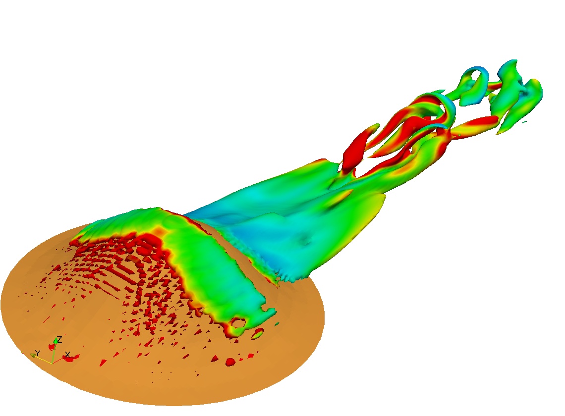
Figure 2: Hairpin eddy structure identified by the objective Q-Criterion with MCT

The symmetric part is the same as the one in NS theory showing the normal expansion of the flow behaviors. However, the physical meaning of the anti-symmetric part, $\Omega_{ij}^{\text{MCT}}$, should be understood as absolute rotation. The off-diagonal part of an anti-symmetric matrix can be represented by a vector. Therefore, one can rewrite the antisymmetric part as a vector of absolute rotation ($\Omega^{\text{AR}}_{k}$), i.e.

$$\Omega^{\text{AR}}_{k} =e_{ijk}\Omega_{ij}^{\text{MCT}}$$

$$=e_{ijk}v_{j,i}-2\omega_{k}$$

$$\sim\nabla\times\vec{v}-2\vec{\omega}$$ (44)

The first half of the $\Omega^{\text{AR}}_{k}$ is vorticity ($\nabla\times\vec{v}$) describing the relative rotation between two inner structure while the second half ($\vec{\omega}$) is the self-spinning of an inner structure. In other words, $\Omega^{\text{AR}}_{k}$ measures the phase shift or the rotational speed difference between the relative rotation and the self-spinning motion. This is the true rotation between two inner structures in a continuum and it does not change even when observed from different reference frames. If $\Omega^{\text{AR}}_{k}$ is zero, it implies that the relative revolution between two inner structures is equal to the self-spinning motion. Therefore, two inner structures always face each other with the same side, like the Earth and the Moon. Without a global coordinate, the inner structure behaves as if there is no motion. Mathematically, $\Omega^{\text{AR}}_{k}=0$ reduces MCT back to NS equations Lopez et al. (2016). This mathematical relation implies that if one believes vorticity can completely resolve all possible rotation without self-spinning gyration, NS theory and MCT are equivalent.

It is noted that Truesdell followed the momumental work by Grad Grad (1952) and derived a balance law of internal rotation Truesdell (1966); Truesdell and Rajapogal (1999). De Groot and Mazur also discussed a similar governing equation in their book De Groot and Mazur (1962). The concept of the internal rotation is similar to the new degrees of freedom, gyration, in MCT. However, De Groot and Mazur derived the balance law from a mechanics perspective so the time evolution of the intrinsic rotation is only governed by the antisymmetric part of Cauchy stress, i.e. $e_{kij}t_{ij}$ in eq. 9. On the other hand, the constitutive equation of gyration in MCT was derived from the classical nonequilibrium thermodynamics. Therefore, there is an additional moment stress, i.e. $m_{lk,l}$ in eq. 9. Consequently, there is a dissipation or diffusion mechanism in the balance law of angular momentum, i.e. $\omega_{k,ll}$ in eq. 23. The diffusion of gyration leads to the heat and eventually the irreversible entropy generation.

Figure 2 shows the iso-surface of the objective Q-Criterion for the coherent eddy structure in the transonic flow over a three-dimensional bump. The iso-surface is colored by the magnitude of the absolute rotation ($\Omega^{\text{AR}}_{k}$). The hairpin structure of the eddies are clearly seen without being limited by the Galilean invariance.

V Conclusion

This work reviews the development of morphing continuum theory from both mathematical and physical perspectives. The complete MCT framework is derived under the framework of rational continuum mechanics for turbulence with subscale eddy structures. A second order finite volume method with second order shock preserving scheme is summarized along with the recent developments on the numerical methods for MCT.

A case of a transonic turbulence over a three-dimensional bump is compared among the MCT, NS and experiments. With less than 10% of the mesh number required in NS-DNS, MCT-DNS provided a better prediction on the pressure coefficient and the pressure profile in the downstream turbulence. It shows that the multiscale MCT does not require the arbitrary fine mesh to resolve the subscale eddy motions. Instead, the subscale eddy motions are captured by the additional degrees of freedom, eg. gyration.

In addition, MCT allows for an objective or frame-indifferent G-criterion for eddy or vortex identifications. The classical NS-based Q-criterion is only Galilean-invariant. It changes when the reference frames becomes time-dependent. The newly proposed MCT-based Q-criterion does not have this limitation and provides sounding results for coherent hairpin eddy structure in the supersonic turbulent flows over a bump.

Future works should be directed at investigating the energy transfer phenomena, shock structure and other essential characterizes in highly compressible turbulence with the multiscale framework of MCT and an affordable computational resources.

References

- Batchelor (1967) G. K. Batchelor, An Introduction to Fluid Dynamics (Cambridge University Press, Cambridge, UK, 1967).
- Eringen (1971) A. C. Eringen, Continuum Physics (Academic Press, New York, NY, 1971).
- Eringen (1980) A. C. Eringen, Mechanics of Continua (Robert E. Krieger, Huntington, NY, 1980).
- Truesdell and Rajapogal (1999) C. Truesdell and K. R. Rajapogal, An Introduction to the Mechanics of Fluids (Birkhauser, Boston, MA, 1999).
- Truesdell (1966) C. Truesdell, Continuum Mechanics I: The Mechanical Functions of Elasticity and Fluid Dynamics (Science, New York, NY, 1966).
- Boltzmann (1964) L. Boltzmann, Lectures on Gas Theory (Dover, New York, NY, 1964).
- Huang (1963) K. Huang, Statistical Mechanics (John Wiley & Sons, New York, NY, 1963).
- Ferziger and Kaper (1972) J. H. Ferziger and H. G. Kaper, Mathematical Theory of Transport Processes in Gases (North Holland, London, UK, 1972).
- Gyarmati (1961a) I. Gyarmati, Periodica Polytechnica. Chemical Engineering 5, 219 (1961a).
- Gyarmati (1961b) I. Gyarmati, Periodica Polytechnica. Chemical Engineering 5, 321 (1961b).
- Li (1967) J. C. M. Li, Physical Review 127, 1784 (1967).
- Coleman and Noll (1963) B. D. Coleman and W. Noll, Archive for Rational Mechanics and Analysis 13, 167 (1963).
- Chen (2013) J. Chen, Acta Mechanica 224, 3153 (2013).
- Müller and Ruggeri (1991) I. Müller and T. Ruggeri, Rational Extended Therdynamics (Springer, 1991).
- Onsager (1931a) L. Onsager, Physical Review 37, 405 (1931a).
- Onsager (1931b) L. Onsager, Physical Review 38, 2265 (1931b).
- De Groot and Mazur (1962) S. R. De Groot and P. Mazur, Non-equilibrium Thermodynamics (North-Holland, Amsterdam, Netherlands, 1962).
- Truesdell (1984) C. Truesdell, Rational Thermodynamics (Springer-Verlag, New York, NY, 1984).
- Haller (2005) G. Haller, Journal of Fluid Mechanics 525, 1 (2005).
- Speziale (1979) C. G. Speziale, Physics of Fluids 22, 1033 (1979).
- Speziale (1987) C. G. Speziale, Physics Review A 36, 4522 (1987).
- Speziale et al. (1991) C. G. Speziale, S. Sarkar, and T. B. Gatski, Journal of Fluid Mechanics 227, 245 (1991).
- Zhong and Wang (2012) X. Zhong and X. Wang, Annual Review of Fluid Mechanics 44, 527 (2012).
- Cosserat and Cosserat (1909) E. Cosserat and F. Cosserat, Thorie des Corps dformables (A. Hermann et Fils, Paris, 1909).
- Eringen (1999) A. C. Eringen, Microcontinuum Field Theories (Springer, New York, NY, 1999).
- Grad (1952) H. Grad, Communications on Pure and Applied Mathematics 5, 455 (1952).
- Snider and Lewchuk (1967) R. F. Snider and K. S. Lewchuk, Journal of Chemical Physics 46, 3163 (1967).
- She and Sather (1967) R. S. C. She and N. F. Sather, Journal of Chemical Physics 47, 4978 (1967).
- Brau (1967) C. A. Brau, Physics of Fluids 10, 48 (1967).
- Curtiss (1992) C. F. Curtiss, Journal of Chemical Physics 97, 1416 (1992).
- Chen (2016) J. Chen, AIAA Paper 2016-4394 (2016).
- Chen (ress) J. Chen, Reports of Mathematical Physics (in press).
- Kirwan and Newman (1969) A. D. Kirwan and N. Newman, International Journal of Engineering Science 7, 883 (1969).
- Liu (1970) C. Y. Liu, International Journal of Engineering Science 8, 457 (1970).
- Eringen and Chang (1970) A. C. Eringen and T. C. Chang, Advances in Materials Science and Engineering 5, 1 (1970).
- Peddieson (1972) J. Peddieson, International Journal of Engineering Science 10, 23 (1972).
- Ahmadi (1975) G. Ahmadi, International Journal of Engineering Science 13, 959 (1975).
- Ahmadi (1981) G. Ahmadi, International Journal of Engineering Science 39, 127 (1981).
- Brutyan and Krapivsky (1992) M. A. Brutyan and P. L. Krapivsky, International Journal of Engineering Science 30, 401 (1992).
- Mehrabian and Atefi (2008) D. Mehrabian and G. Atefi, Journal of Dispersion Science and Technology 29, 1035 (2008).
- Alizadeth et al. (2011) M. Alizadeth, G. Silber, and A. G. Nejad, Journal of Dispersion Science and Technology 32, 185 (2011).
- Chen et al. (2010) J. Chen, C. Liang, and J. D. Lee, Journal of Nanoengineering and Nanosystems 224, 31 (2010).
- Chen et al. (2012) J. Chen, C. Liang, and J. D. Lee, Computers & Fluids 66, 1 (2012).
- Crnjavic-Zic and Mujakovic (2016) N. Crnjavic-Zic and N. Mujakovic, Mathematics and Computers in Simulation 126, 45 (2016).
- Drazic et al. (2017) I. Drazic, N. Mujakovic, and N. Crnjavic-Zic, Journal of Mathematical Analysis and Applications 449, 1637–1669 (2017).
- Wonnell and Chen (2016) L. B. Wonnell and J. Chen, AIAA Paper 2016-4279 (2016).
- Wonnell and Chen (2017a) L. B. Wonnell and J. Chen, Journal of Fluids Engineering 139, 011205 (2017a).
- Cheikh and Chen (2017) M. I. Cheikh and J. Chen, AIAA Paper 2017-3460 (2017).
- Wonnell and Chen (2017b) L. B. Wonnell and J. Chen, AIAA Paper 2017-3461 (2017b).
- Chen et al. (2011) J. Chen, J. D. Lee, and C. Liang, Journal of Non-Newtonian Fluid Mechanics 166, 867 (2011).
- Mordant et al. (2001) N. Mordant, P. Metz, O. Michel, and J.-F. Pinton, Physical Review Letters 87, 214501 (2001).
- Ryabtsev et al. (2016) A. Ryabtsev, S. Pouya, A. Safaripour, M. M. Koochesfahani, and H. Dantus, Optics Express 24, 11762 (2016).
- Panton (2013) R. L. Panton, Incompressible Flow (Wiley, Hoboken, NJ, 2013).
- Eringen (2001) A. C. Eringen, Microcontinuum Field Theories II: Fluent Media (Springer-Verlag, New York, NY, 2001).
- Feynman et al. (1970) R. Feynman, R. Leighton, and M. Sand, The Feynman Lectures on physics (Addison Wesley Longman, New York, NY, 1970).
- Edelen (1972) D. Edelen, International Journal of Engineering Science 10, 481 (1972).
- Wang (1969) C.-C. Wang, Archive for Rational Mechanics and Analysis 36, 166 (1969).
- Wang (1970) C.-C. Wang, Archive for Rational Mechanics and Analysis 43, 392 (1970).
- ilhavý (1997) M. ilhavý, The Mechanics and Thermodynamics of Continuous Media (Springer, 1997).
- Berezovski and Van (2017) A. Berezovski and P. Van, Internal Variables in Thermoelasticity (Springer, 2017).
- Patankar (1984) S. V. Patankar, Numerical Heat Transfer and Fluid Flow (Taylor & Francis, 1984).
- Liu et al. (2006a) Y. Liu, M. Vinokur, and Z. J. Wang, Journal of Computational Physics 216, 780 (2006a).
- Wang et al. (2007) Z. Wang, Y. Liu, G. May, and A. Jameson, Journal of Scientific Computing 32, 45 (2007).
- Wang (2002) Z. J. Wang, Journal of Computational Physics 178, 210 (2002).
- Liu et al. (2006b) Y. Liu, M. Vinokur, and Z. J. Wang, Journal of Computational Physics 212, 454 (2006b).
- Nishikawa and Liu (2017) H. Nishikawa and Y. Liu, Journal of Computational Physics 344, 595 (2017).
- Mujakovic and Crnjaric-Zic (2015) N. Mujakovic and N. Crnjaric-Zic, Internatoinal Journal of Numerical Analysis and Modeling 12, 94 (2015).
- Kurganov et al. (2001) A. Kurganov, S. Noelle, and G. Petrov, SIAM Journal of Scientific Computing 23, 707 (2001).
- Simpson et al. (2002) R. L. Simpson, C. H. Long, and G. Byun, International Journal of Heat and Fluid Flow 23, 582 (2002).
- Castagna et al. (2014) J. Castagna, Y. Yao, and J. Yao, Computers & Fluids 95, 116 (2014).
- Speziale (1989) C. G. Speziale, Theoretical and Computaiotnal Fluid Dynamics 1, 3 (1989).
- Speziale (1998) C. G. Speziale, Applied Mechanics Reviews 51, 489 (1998).
- Lopez et al. (2016) M. Lopez, J. Chen, and V. A. Palochko, Molecular Simulation 42, 1370 (2016).