Hidden Markov model tracking of continuous gravitational waves from a binary neutron star with wandering spin. II. Binary orbital phase tracking

Abstract

A hidden Markov model (HMM) scheme for tracking continuous-wave gravitational radiation from neutron stars in low-mass X-ray binaries (LMXBs) with wandering spin is extended by introducing a frequency-domain matched filter, called the $\mathcal{J}$-statistic, which sums the signal power in orbital sidebands coherently. The $\mathcal{J}$-statistic is similar but not identical to the binary-modulated $\mathcal{F}$-statistic computed by demodulation or resampling. By injecting synthetic LMXB signals into Gaussian noise characteristic of the Advanced Laser Interferometer Gravitational-wave Observatory (Advanced LIGO), it is shown that the $\mathcal{J}$-statistic HMM tracker detects signals with characteristic wave strain $h_{0}\geq 2\times 10^{-26}$ in 370 d of data from two interferometers, divided into 37 coherent blocks of equal length. When applied to data from Stage I of the Scorpius X-1 Mock Data Challenge organised by the LIGO Scientific Collaboration, the tracker detects all 50 closed injections ($h_{0}\geq 6.84\times 10^{-26}$), recovering the frequency with a root-mean-square accuracy of $\leq 1.95\times 10^{-5}\,\mathrm{Hz}$. Of the 50 injections, 43 (with $h_{0}\geq 1.09\times 10^{-25}$) are detected in a single, coherent 10-d block of data. The tracker employs an efficient, recursive HMM solver based on the Viterbi algorithm, which requires $\sim 10^{5}$ CPU-hours for a typical, broadband (0.5-kHz), LMXB search.

[Version 6.21]

I Introduction

Continuous-wave gravitational radiation from accreting neutron stars in binary systems is a key target of long-baseline interferometers like the Laser Interferometer Gravitational Wave Observatory (LIGO) and Virgo in the Advanced Detector Era (Riles, 2013). In particular, X-ray–emitting neutron stars in low-mass X-ray binaries (LMXBs) are predicted to be relatively strong sources if they exist in a state of torque balance (Wagoner, 1984; Bildsten, 1998). The characteristic gravitational wave strain $h_{0}$ emitted by an LMXB in torque balance is proportional to the square root of the X-ray flux independent of the distance to the source. (Bildsten, 1998) Scorpius X-1 (Sco X-1), the brightest LMXB in X-rays, is therefore the highest priority target in this class. Several plausible mechanisms exist for generating the mass or current quadrupole moment required for torque balance, ranging from thermocompositional and magnetic mountains (Ushomirsky et al., 2000; Melatos and Payne, 2005; Vigelius and Melatos, 2009; Priymak et al., 2011) to $r$-modes (Owen et al., 1998; Bondarescu et al., 2007; Bondarescu and Wasserman, 2013). Even without torque balance, the prospects of detecting LMXBs with persistent X-ray emission are encouraging, depending on the detailed physics of deep crustal heating (Haskell et al., 2015).

A nonaxisymmetric rotor in a Keplerian orbit emits a frequency-modulated gravitational wave signal. The orbital Doppler shift disperses the emitted power into Fourier sidebands separated in frequency by $P^{-1}$, where $P$ is the orbital period. Several strategies have been deployed previously to process signals of this kind. The TwoSpect algorithm, which operates on doubly-Fourier-transformed data, was used to conduct an all-sky search for unknown binaries in data from LIGO Science Run 6 (S6) and Virgo Science Runs 2 and 3 (VSR2 and VSR3 respectively), returning upper limits of $h_{0}\lesssim 2\times 10^{-24}$ for a whole sky search at $217\,\mathrm{Hz}$ and $h_{0}\lesssim 1\times 10^{-23}$ for a search of the frequency range 20–57 Hz for Sco X-1 (Aasi et al., 2014a; Goetz and Riles, 2011). A fully templated version of TwoSpect, tailored to handle directed LMXB searches, offers substantial computational savings (Meadors et al., 2016). The sideband algorithm, which sums the power in the orbital sidebands of the maximum-likelihood $\mathcal{F}$-statistic semi-coherently, was used to conduct a directed search for Sco X-1 in LIGO Science Run 5 (S5) data, returning an upper limit of $h_{0}\leq 8\times 10^{-25}$ at $150\,\mathrm{Hz}$ (Aasi et al., 2015a; Sammut et al., 2014; Messenger and Woan, 2007). The radiometer algorithm applied to LIGO S5 data returns a model-independent upper limit of $5\times 10^{-25}$ for the root-mean-square wave strain across a $0.25\,\mathrm{Hz}$ bin at $160\,\mathrm{Hz}$ at the sky position of Sco X-1 (Abadie et al., 2011; Ballmer, 2006). The cross-correlation algorithm, which multiplies Fourier transforms in pairs weighted by a phase with an adjustable time lag (Dhurandhar et al., 2008; Chung et al., 2011; Whelan et al., 2015; Sun et al., 2016), and the polynomial algorithm (van der Putten et al., 2010) have not yet been applied to actual interferometer data in a Sco X-1 search but they competed in Stage I of the Sco X-1 Mock Data Challenge (MDC) (Messenger et al., 2015), together with the TwoSpect, sideband, and radiometer algorithms. Parameter-space metrics for binary sources, a key ingredient for building semi-coherent StackSlide-type search pipelines, have been derived recently (Leaci and Prix, 2015) and used to estimate the optimal sensitivity of a general semi-coherent search for Sco X-1 in the Advanced Detector Era.

A key challenge facing LMXB searches is that the spin frequency of the source, and hence its gravitational wave frequency, wander stochastically. Spin wandering, which is observed in X-ray pulsar timing experiments (Bildsten et al., 1997), is driven by fluctuations in the hydromagnetic accretion torque (Baykal and Oegelman, 1993; de Kool and Anzer, 1993; Romanova et al., 2004) due to transient accretion disk formation (Taam and Fryxell, 1988; Baykal et al., 1991) or disk-magnetosphere instabilities (Romanova et al., 2004). It is auto-correlated on time-scales of days to weeks (Baykal, 1997). Recent work by Suvorova et al. (2016) demonstrates that hidden Markov model (HMM) methods offer a practical, computationally efficient strategy for tracking a wandering frequency (Quinn and Hannan, 2001). HMM methods have been deployed with success in many engineering applications, ranging from radar and sonar analysis (Paris and Jauffret, 2003) to mobile telephony (White and Elliott, 2002). They deliver accurate estimation, when the signal-to-noise ratio (SNR) is low, but the sample size is large (Quinn and Hannan, 2001), as is the case for continuous-wave searches for gravitational radiation from neutron stars in binary systems. Suvorova et al. (2016) implemented and tested a HMM scheme based on a Bessel-weighted variant of the maximum-likelihood $\mathcal{F}$-statistic and the classic Viterbi HMM scheme (Quinn and Hannan, 2001; Viterbi, 1967). The scheme successfully detects synthetic, spin-wandering, binary signals with $h_{0}\gtrsim 8\times 10^{-26}$ in Gaussian noise with power spectral density $4\times 10^{-24}\,\mathrm{Hz}^{-1/2}$. It also detects 41 out of 50 signals without spin wandering in Stage I of the Sco X-1 MDC with $h_{0}\geq 1.1\times 10^{-25}$, achieving root-mean-square accuracy $\leq 4\times 10^{-3}\,\mathrm{Hz}$ in frequency estimation. A directed search of LIGO Observing Run 1 (O1) data in the range 60–650 Hz with the HMM scheme reported an upper limit of $h_{0}\lesssim 8\times 10^{-25}$, and had a computational cost of $\sim 10^{3}$ CPU-hr (The LIGO Scientific Collaboration et al., 2017).

In this paper, we report on an improved version of the above HMM scheme, which achieves better sensitivity while remaining competitive in terms of computational cost. In Ref. (Suvorova et al., 2016), the detection statistic at each HMM step is calculated by summing the $\mathcal{F}$-statistic values at orbital sidebands weighted by positive coefficients proportional to the squares of Bessel functions. Physically this corresponds to summing the sideband powers incoherently, i.e. neglecting the relative phases of the sideband spectral components. In this paper, we replace the above detection statistic with a variant, called the $\mathcal{J}$-statistic, that preserves the orbital phase information. The rest of the analysis pipeline remains unchanged, i.e. we solve the HMM recursively using the Viterbi algorithm as in previous work. The $\mathcal{J}$-statistic takes as an input the initial orbital phase (or equivalently the time of passage through the orbit’s ascending node or the epoch of inferior conjunction) (Sammut et al., 2014). This information is typically measured for LMXBs to an accuracy of $\lesssim 10^{-2}\,\mathrm{rad}$ from contemporary and historical optical spectroscopic data (Premachandra et al., 2016; Galloway et al., 2014). A refined measurement is returned by the algorithm itself in the event of a detection.

The paper is structured as follows. In Section II, we review briefly the HMM framework for frequency tracking and the Viterbi algorithm implemented to solve the HMM. In Section III, we introduce the $\mathcal{J}$-statistic and show how it follows naturally from the phase model of the source. The $\mathcal{J}$-statistic is constructed from the same intermediate data products as the $\mathcal{F}$-statistic, leveraging existing and thoroughly tested software infrastructure built by the LIGO Scientific Collaboration. The improved HMM pipeline is tested against synthetic data with Gaussian noise in Section IV and data from Stage I of the Sco X-1 MDC in Section V.

II Frequency tracking

In this section we review briefly the HMM approach to frequency tracking, as applied to continuous-wave searches (Section IIA), and the classic Viterbi algorithm for solving the resulting HMM scheme (Section IIB). The reader is referred to Ref. (Suvorova et al., 2016) and references therein for a full description of the method and its implementation. We copy the notation from Ref. (Suvorova et al., 2016) in what follows.

II.1 HMM framework

Let $f_{\star}(t)$ be the unknown, wandering spin frequency of the neutron star as a function of time $t$. An HMM models the time series $f_{\star}(t)$ as a sequence of random jumps between unobservable (‘hidden’) states, which are themselves related probabilistically to some observable quantity (here, the interferometer data) via a detection statistic. The objective of an HMM analysis is to find the most likely sequence of jumps consistent with the observations, once the transition probabilities are prescribed.

Continuous-wave searches are typically performed in the frequency domain on interferometer data that have been packaged into short Fourier transforms (SFTs) of duration $T_{\mathrm{SFT}}=30\,\mathrm{min}$, during which $f_{\star}(t)$ remains confined to one frequency bin of width $\Delta f_{\mathrm{SFT}}=(2T_{\mathrm{SFT}})^{-1}$. Consecutive SFTs are combined to compute a frequency-domain detection statistic $G(f)$. In between $T_{\mathrm{SFT}}$ and the total observation time $T_{\mathrm{obs}}$, for any particular astrophysical source, one can always calculate $G(f)$ over an intermediate ‘drift’ time-scale $T_{\mathrm{drift}}$ ($T_{\mathrm{SFT}}\leq T_{\mathrm{drift}}\leq T_{\mathrm{obs}}$), such that $f_{\star}(t)$ remains confined within one $G(f)$ frequency bin of width $\Delta f_{\mathrm{drift}}=(2T_{\mathrm{drift}})^{-1}$, viz.

$$\left|\int_{t}^{t+T_{\mathrm{drift}}}\,\mathrm{d}t^{\prime}\,\dot{f}_{\star}(t^{\prime})\right|<\Delta f_{\mathrm{drift}}$$ (1)

for all $t$. For example, in the published sideband search for Sco X-1 in LIGO S5 data, 480 consecutive SFTs are combined to compute the sideband $\mathcal{C}$-statistic $\mathcal{C}(f)$ for $T_{\mathrm{drift}}=10\,\mathrm{d}$, under the assumption that $f_{\star}(t)$ wanders by less than $\Delta f_{\mathrm{drift}}=6\times 10^{-7}\,\mathrm{Hz}$ during that time interval (Sammut et al., 2014; Aasi et al., 2015a).

In an HMM search, we compute $G(f)$ for $N_{T}=T_{\mathrm{obs}}/T_{\mathrm{drift}}$ blocks of data. In each block, the discretised hidden variable $q(t)=f_{\star}(t)$ is constant and occupies one of $N_{f_{\star}}=B/\Delta f_{\mathrm{drift}}$ discrete hidden states $\{q_{1},...,q_{N_{f_{\star}}}\}$, where $B=f_{\star,\mathrm{max}}-f_{\star,\mathrm{min}}$ is the total search bandwidth. As the HMM steps from one block to the next, $q(t)$ jumps from one discrete state to another. For a source in a binary, $G(f)$ depends not only on $f_{\star}$ but also on the projected semimajor axis of the binary orbit, $a_{0}=a\sin i$, and the orbital phase $\phi_{a}$ at a reference time $t_{a}$ (here the time of passage through the ascending node). Optical spectroscopy measures $a_{0}$ and $\phi_{a}$ to accuracies of $\sim 25\%$ and $\sim 1\%$ respectively (see Section IV.4 for further discussion). (Galloway et al., 2014; Premachandra et al., 2016) Typically these resolutions are too coarse to produce a detectable peak in $G(f)$ and hence the HMM output; see Figure 7 in Ref. (Suvorova et al., 2016). Hence one must normally subdivide $a_{0}$ and $\phi_{a}$ more finely and track a three-dimensional hidden state variable $q(t)=[f_{\star}(t),a_{0}(t),\phi_{a}(t)]$, which can take on $N_{Q}=N_{f_{\star}}N_{a_{0}}N_{\phi_{a}}$ possible values, where each $a_{0}$ ($\phi_{a}$) bin has width $\Delta a_{0}=2\sigma_{a_{0}}/N_{a_{0}}$ ($\Delta\phi_{a}=2\sigma_{\phi_{a}}/N_{\phi_{a}}$), and $\sigma_{a_{0}}$ ($\sigma_{\phi_{a}}$) is the one–standard-deviation error bar on $a_{0}$ ($\phi_{a}$) from electromagnetic observations. Under normal astrophysical conditions, $a_{0}$ and $\phi_{a}$ are constant during the full search ($T_{\mathrm{obs}}\lesssim 1\,\mathrm{yr}$), and the three-dimensional HMM reduces to its one-dimensional counterpart [with $q(t)=f_{\star}(t)$] computed on a grid of $N_{a_{0}}N_{\phi_{a}}$ pairs $(a_{0},\phi_{a})$. We adopt the latter approach, which is readily parallelisable, in this paper.

For a Markov process, the jump probability for the time step $t_{n}$ to $t_{n+1}$ depends only on $q(t_{n})$ and is described by the transition probability matrix

$$A_{q_{j}q_{i}}=\Pr\left[q(t_{n+1})=q_{j}\mid q(t_{n})=q_{i}\right],$$ (2)

where $q_{i}$ and $q_{j}$ are single-index labels enumerating $N_{Q}$ discrete states. As in Ref. (Suvorova et al., 2016), we approximate spin wandering as an unbiased random walk or Weiner process: at every time step, $f_{\star}(t)$ jumps by $0$ or $\pm 1$ frequency bins with equal probability in the absence of discontinuous glitches (Bildsten et al., 1997). As noted above, for observations with $T_{\mathrm{obs}}\lesssim 1\,\mathrm{yr}$, much shorter than the mass transfer time-scale ($T_{\mathrm{acc}}\sim 10^{7}\,\mathrm{yr}$), the orbital elements are constant up to negligible corrections of order $T_{\mathrm{obs}}/T_{\mathrm{acc}}$, and the HMM is effectively one-dimensional, with $q(t)=f_{\star}(t)$ and $N_{Q}=N_{f_{\star}}$. Hence the transition probabilities take the simple form

$$A_{q_{j}q_{i}}=\frac{1}{3}\left(\delta_{q_{j},q_{i+1}}+\delta_{q_{j},q_{i}}+\delta_{q_{j},q_{i-1}}\right),$$ (3)

where $\delta_{ij}$ symbolises the Kronecker delta. Other choices of the weights, e.g $\frac{1}{4}$, $\frac{1}{2}$, $\frac{1}{4}$ are possible, but testing shows there is little difference in performance. Machine learning techniques for determining the weights from the data are also possible but are beyond the scope of this paper (Baum et al., 1970).

In a continuous-wave search, the observable state variable $o(t)$ corresponds to the data collected during the interval $t\leq t^{\prime}\leq t+T_{\mathrm{drift}}$. Formally it is a vector, whose dimension equals the interferometer sampling frequency multiplied by $T_{\mathrm{drift}}$. The probability that the system is observed in state $o(t_{n})$ at time $t_{n}$ while it occupies the hidden state $q(t_{n})$ is called the emission probability,

$$L_{o_{j}q_{i}}=\mathrm{Pr}\left[o(t_{n})=o_{j}\mid q(t_{n})=q_{i}\right]$$ (4)

In the class of continuous-wave searches considered in this paper, $L_{o_{j}q_{i}}$ can be expressed in terms of the frequency domain detection statistic $G(f)$ as

$$L_{o(t_{n})q_{i}}\propto\exp[G(f_{\star i})],$$ (5)

where $G(f_{\star i})$ is the log likelihood that $f_{\star}(t^{\prime})$ lies in the $i$-th frequency bin $\left[f_{\star i},f_{\star i}+\Delta f_{\mathrm{drift}}\right]$ during the interval $t_{n}\leq t^{\prime}\leq t_{n}+T_{\mathrm{drift}}$. We derive another version of $G(f)$, called the $\mathcal{J}$-statistic, in Section III, which generalises the estimator in Ref. (Suvorova et al., 2016) by summing the power in orbital sidebands coherently with respect to orbital phase.

Given an observed sequence $O=\left[o(t_{0}),...,o(t_{N_{T}})\right]$, there exist $N_{Q}^{N_{T}+1}$ hidden sequences $Q=\left[q(t_{0}),...,q(t_{N_{T}})\right]$, which can give rise to $O$. Assuming the Markov property, each hidden sequence has probability

$$\mathrm{P}(Q|O) =L_{o(t_{N_{T}})q(t_{N_{T}})}A_{q(t_{N_{T}})q(t_{N_{T}-1})}\cdots L_{o(t_{1})q(t_{1})}$$

$$\phantom{=}\times A_{q(t_{1})q(t_{0})}\Pi_{q(t_{0})},$$ (6)

where

$$\Pi_{q_{i}}=\mathrm{Pr}[q(t_{0})=q_{i}]$$ (7)

is the prior probability of each hidden state, which we take to be uniform for simplicity, viz.

$$\Pi_{q_{i}}=N_{Q}^{-1}.$$ (8)

The most probable path $Q^{\star}(O)=\operatorname*{arg\,max}\mathrm{Pr}(Q|O)$, i.e., the path that maximises equation (6), represents the HMM’s best estimate of the spin history $f_{\star}(t)$ of the source.

II.2 Viterbi algorithm

Many methods exist to solve efficiently for $Q^{\star}(O)$; see Ref. (Quinn and Hannan, 2001) for examples. The challenge is to prune the $N_{Q}^{N_{T}+1}$ possible hidden sequences in an efficient way. One approach, first proposed by Viterbi (1967), takes advantage of the Markov property, and the fact that subsequences of the optimal sequence $Q^{\star}(O)$ are themselves optimal, to find $Q^{\star}(O)$ recursively by backtracking. At every forward step in the recursion, the Viterbi algorithm eliminates all but $N_{Q}$ possible state sequences; overall its computational cost is $(N_{T}+1)N_{Q}\ln N_{Q}$ (Quinn and Hannan, 2001).

At forward step $k$ ($1\leq k\leq N_{T}$), we calculate and store the $N_{Q}$ maximum probabilities

$$\delta_{q_{i}}(t_{k})=L_{o(t_{k})q_{i}}\max_{1\leq j\leq N_{Q}}\left[A_{q_{i}q_{j}}\delta_{q_{j}}(t_{k-1})\right]$$ (9)

and the states

$$\Phi_{q_{i}}(t_{k})=\operatorname*{arg\,max}_{1\leq j\leq N_{Q}}\left[A_{q_{i}q_{j}}\delta_{q_{j}}(t_{k-1})\right]$$ (10)

from which each maximum probability is reached, with $1\leq i\leq N_{Q}$. The optimal path is then reconstructed by backtracking for $0\leq k\leq N_{T}-1$:

$$q^{\star}(t_{k})=\Phi_{q^{\star}(t_{k+1})}(t_{k+1})$$ (11)

Hence, the Viterbi algorithm computes the maximum likelihood estimator, i.e., $\operatorname*{arg\,max}\Pr(Q|O)$.

Detailed pseudocode for the algorithm, including the initialisation and termination steps, is given in Ref. (Suvorova et al., 2016), following the notation and presentation in the textbook by Quinn and Hannan (2001).

III Matched filter

The emission probability $L_{o(t)q_{i}}$ is computed from the frequency domain estimator $G(f)$ according to equation (5). Many valid choices exist for $G(f)$, depending on computational constraints, the format of the interferometer data, and the assumed model for the phase evolution of the source. In this paper, we leverage the existing software infrastructure for continuous-wave searches in the LIGO Scientific Collaboration Algorithm Library (LAL) to build $G(f)$ out of the easy-to-use and thoroughly tested maximum-likelihood matched filter called the $\mathcal{F}$-statistic (Jaranowski et al., 1998). We review the $\mathcal{F}$-statistic for an isolated source without any orbital motion in Section III.1. We then describe in Section III.2 a method to combine $\mathcal{F}$-statistic values at orbital sidebands coherently — by tracking orbital phase — to construct a matched filter for a binary source. The latter version of $G(f)$, termed the $\mathcal{J}$-statistic, is compared with incoherent algorithms for summing orbital sidebands like the $\mathcal{C}$-statistic (Messenger and Woan, 2007; Sammut et al., 2014; Aasi et al., 2015b) and Bessel-weighted $\mathcal{F}$-statistic (Suvorova et al., 2016) in Section III.3.

III.1 Isolated source: $\mathcal{F}$-statistic

The gravitational wave signal from a biaxial rotor without any orbital motion can be written in the form

$$h(t)=\sum_{i=1}^{4}A_{1i}h_{1i}(t),+A_{2i}h_{2i}(t).$$ (12)

The independent components $h_{1i}(t)$ are given by

$$h_{11}(t) =a(t)\cos\Phi(t),$$ (13)

$$h_{12}(t) =b(t)\cos\Phi(t),$$ (14)

$$h_{13}(t) =a(t)\sin\Phi(t),$$ (15)

$$h_{14}(t) =b(t)\sin\Phi(t),$$ (16)

where $\Phi(t)$ is the signal phase at the detector and $h_{2i}(t)$ is obtained from $h_{1i}(t)$ by replacing $\Phi(t)$ with $2\Phi(t)$ in equations (13)–(16). In (12)–(16), $A_{1i}$ and $A_{2i}$ denote arbitrary amplitudes specific to the source, and $a(t)$ and $b(t)$ are antenna beam-pattern functions defined by equations (12) and (13) in Ref. (Jaranowski et al., 1998), which contain information about the source’s sky position (right ascension $\alpha$, declination $\delta$), the Earth’s rotation and the detector’s orientation. Following equations (18) and (96) in Ref. (Jaranowski et al., 1998), we split the signal phase into three terms,

$$\Phi(t)=2\pi f_{\star}[t+\Phi_{m}(t;\alpha,\delta)]+\Phi_{s}[t;f_{\star}^{(k)},\alpha,\delta],$$ (17)

where $\Phi_{m}$ is a time shift produced by the diurnal and annual motions of the detector and source relative to the Solar System barycentre (SSB), and $\Phi_{s}$ is a phase shift combining the latter two effects with the intrinsic evolution of the source in its own rest frame through the intrinsic frequency derivatives $f_{\star}^{(k)}=d^{k}\!f_{\star}/dt^{k}$ (with $k\geq 1$).

The output from a single interferometer is given by $x(t)=h(t)+n(t)$, where $n(t)$ denotes additive noise. Consider the special case $A_{2i}=0$. If the noise is Gaussian, then the normalised log likelihood of measuring the time series $x(t)$ over the interval $0\leq t\leq T_{\mathrm{obs}}$ is proportional to

$$\ln\Lambda^{\prime}_{1}=(x||h)-\tfrac{1}{2}(h||h),$$ (18)

where we define the inner product

$$(x||y)=\frac{2}{T_{\mathrm{obs}}}\int_{0}^{T_{\mathrm{obs}}}\,\mathrm{d}t\,x(t)y(t).$$ (19)

Maximising $\ln\Lambda^{\prime}_{1}$ with respect to the four amplitudes $A_{1i}$, we arrive at the following expression for the maximum-likelihood matched filter known as the $\mathcal{F}$-statistic,

$$\mathcal{F} =D^{-1}[B(x||h_{11})^{2}-2C(x||h_{11})(x||h_{12})+A(x||h_{12})^{2}$$

$$\phantom{=}+B(x||h_{13})^{2}-2C(x||h_{13})(x||h_{14})+A(x||h_{14})^{2}],$$ (20)

with $A=(a||a)$, $B=(b||b)$, $C=(a||b)$ and $D=AB-C^{2}$. When searching the data $x(t)$ for a gravitational wave signal, we evaluate $\mathcal{F}$ as a function of the source parameters, e.g., $f_{\star}$, $\alpha$, $\delta$, some or all of which may not be known. A similar, independent maximisation procedure may be performed to solve for the amplitudes $A_{2i}$. The result is identical to (III.1), except that $h_{1i}$ is replaced by $h_{2i}$.

In practice, LIGO continuous-wave searches often take Fourier-transformed interferometer data as inputs. It is therefore convenient to rewrite the inner product (19) in terms of the Fourier transform of $x(t)$. The calculation is presented in detail in Section IIID of Ref. (Jaranowski et al., 1998) and also in Ref. (Prix, 2011). Here we quote the result. Let $f_{0}$ be the search frequency, where the $\mathcal{F}$-statistic is evaluated, which may or may not coincide with the star’s spin frequency $f_{\star}$. For $f_{0}\neq f_{\star}$ we have $\left\langle\mathcal{F}(f_{0})=0\right\rangle$ and $\left\langle|\mathcal{F}(f_{0})|^{2}\right\rangle\approx S_{h}(f_{0})T_{\mathrm{obs}}$, where $\langle\cdots\rangle$ denotes an ensemble average over many realisations of the noise, and $S_{h}(f_{0})$ denoted the one-sided noise power spectral density at frequency $f_{0}$. For $f_{0}=f_{\star}$, we have $\left\langle\mathcal{F}(f_{0})=0\right\rangle$ and $\left\langle|\mathcal{F}(f_{0})|^{2}\right\rangle\gtrsim h_{0}^{2}T_{\mathrm{obs}}^{2}$. Define the Fourier integral

$$\mathcal{F}_{1a}=\int_{0}^{T_{\mathrm{obs}}}\,\mathrm{d}t_{b}\,x[t(t_{b})]a[t(t_{b})]e^{-i\Phi_{s}[t(t_{b})]}e^{-2\pi if_{0}t_{b}},$$ (21)

and define $\mathcal{F}_{1b}$ in the same way but with $a[t(t_{b})]$ replaced by $b[t(t_{b})]$. We can then rewrite (III.1) as

$$\mathcal{F}=\frac{4}{S_{h}(f_{0})T_{\mathrm{obs}}D}\left[B|\mathcal{F}_{1a}|^{2}-2C\mathrm{Re}(\mathcal{F}_{1a}\mathcal{F}_{1b}^{\star})+A|\mathcal{F}_{1b}|^{2}\right]$$ (22)

after rescaling by a factor $T_{\mathrm{obs}}/S_{h}(f_{0})$ as in equation (56) in Ref. (Jaranowski et al., 1998). In (21), $t_{b}=t+\Phi_{m}(t)$ denotes a new barycentered time coordinate related implicitly to $t$ through the time shift introduced by the Earth’s rotation and revolution.

Formally, equation (21) integrates all the data, implying a Fourier transform with $\sim 10^{10}$ points for $T_{\mathrm{obs}}=1\,\mathrm{yr}$ and kilohertz sampling. In practice, to assist with storage, the integral is subdivided into ‘atoms’ (Prix, 2011). Each atom corresponds to one SFT and is labelled by $X\alpha$, where $X$ indexes the interferometer, and $\alpha$ is the ordinal of the SFT for that interferometer. If the SFT labelled by $X\alpha$ runs over the interval $t_{X\alpha}\leq t\leq t_{X\alpha}+T_{\mathrm{SFT}}$, equation (21) simplifies to

$$\mathcal{F}_{1a}=\sum_{X\alpha}\hat{a}_{X\alpha}\int_{t_{X\alpha}}^{t_{X\alpha}+T_{\mathrm{SFT}}}\,\mathrm{d}t_{b}\,x[t(t_{b})]e^{-i\Phi_{s}[t(t_{b})]}e^{-2\pi if_{0}t_{b}}$$ (23)

with

$$\hat{a}_{X\alpha}=a[t(t_{b}=t_{X\alpha}+T_{\mathrm{SFT}}/2)].$$ (24)

We make the approximation in equations (23) and (24) that $a(t)$, which has a 24-hr period, changes slowly during the 30-min SFT (typically without switching sign) and can be approximated by its midpoint value. In order to convert an SFT (frequency bin width $\Delta f_{\mathrm{SFT}}$) into atom-based quantities like $\mathcal{F}_{1a}$, $\mathcal{F}_{1b}$ and $\mathcal{F}$ (frequency bin width $\Delta f_{\mathrm{drift}}=T_{\mathrm{SFT}}\Delta f_{\mathrm{SFT}}/T_{\mathrm{drift}}\ll\Delta f_{\mathrm{SFT}}$), we ‘fill in’ the intermediate bins according to the Williams-Schutz approximation by convolving with the sinc function associated with the Fourier transform of the window $t_{X\alpha}\leq t\leq t_{X\alpha}+T_{\mathrm{SFT}}$. The reader is referred to Section 4.2 of Ref. (Prix, 2011) for full details.

III.2 Binary source: $\mathcal{J}$-statistic

The gravitational wave signal from a biaxial rotor in a Keplerian orbit is given by equations (12)–(16), as for an isolated source, except that the observed frequency is modulated by the orbital Doppler shift, and the phase varies harmonically as

$$\Phi_{s}(t)=-2\pi f_{\star}a_{0}\sin\Omega(t-t_{a}),$$ (25)

where $a_{0}$ is the projected semimajor axis, $\Omega=2\pi/P$ is the orbital angular velocity, $P$ is the orbital period, and $t_{a}=\phi_{a}/\Omega$ is a reference time, usually taken to be the time of passage through the ascending node. The phase model (25) assumes a circular orbit for simplicity; a nonzero orbital eccentricity is straightforward to include in the fashion described in Section 4.5 of Ref. (Sammut et al., 2014). Intrinsic, nonorbital frequency derivatives $f_{\star}^{(k)}$ are also omitted from (25) but are implemented as options in the LAL $\mathcal{F}$-statistic code and can be activated easily via a software switch.

Upon substituting (25) with $f_{\star}$ replaced by $f_{0}$ into (23) and expanding the factor $e^{-i\Phi_{s}[t(t_{b})]}$ with the aid of the Jacobi-Anger identity, we obtain the Fourier integral

$$\mathcal{J}_{1a} =\sum_{X\alpha}\sum^{\infty}_{s=-\infty}\hat{a}_{X\alpha}J_{s}(2\pi f_{0}a_{0})e^{-is\phi_{a}}$$

$$\phantom{=}\times\int_{t_{X\alpha}}^{t_{X\alpha}+T_{\mathrm{SFT}}}\,\mathrm{d}t_{b}\,x[t(t_{b})]e^{-2\pi i(f_{0}-s/P)t_{b}}.$$ (26)

The $\mathcal{J}$-statistic is then obtained by evaluating (22) using (26) and an analogous formula for $\mathcal{J}_{1b}$. The sum over Bessel orders is truncated to $M=2\mathrm{ceil}(2\pi f_{0}a_{0})+1$ terms, because we have $|J_{s}(2\pi f_{0}a_{0})|\ll 1$ for $|s|>2\pi f_{0}a_{0}\gg 1$.

The second line in (26) is the same windowed Fourier transform calculated by the $\mathcal{F}$-statistic, with $f_{0}^{(k)}=0$ for all $k\geq 1$, evaluated at $f_{0}-s/P$ instead of $f_{0}$. Hence we can compute the $\mathcal{J}$-statistic using existing $\mathcal{F}$-statistic infrastructure by summing the $\mathcal{F}$-statistic output at orbital sidebands weighted by a phase factor $\propto e^{-is\phi_{a}}$. Strictly speaking, according to Ref. (Jaranowski et al., 1998), $\Phi_{s}$ in (17) is allowed to depend on $f_{0}^{(k)}$ for $k\geq 1$ but not on $f_{0}$ itself. We may therefore elect to replace $f_{0}$ by its average value $\bar{f_{0}}$ across a narrow sub-sideband (of width $1\,\mathrm{Hz}$, say) in the argument of $J_{s}$, as in previous analyses using the $\mathcal{C}$-statistic (Sammut et al., 2014; Aasi et al., 2015b). It is found a posteriori that the results are nearly indistinguishable. In the previous HMM study involving the Bessel-weighted $\mathcal{F}$-statistic, where the data are convolved with a Bessel filter, $f_{0}$ is replaced by $\bar{f_{0}}$ in $1$-Hz sub-bands to avoid recalculating the filter in every one of $N_{f_{\star}}$ frequency bins, realising computational savings (Suvorova et al., 2016). Accordingly, a search of a large band will be implemented as a series of searches over overlapping, $1$-Hz sub-bands.

Long-term optical spectroscopy measures $t_{a}$ to an accuracy of $|\Delta t_{a}|\sim 10^{-3}P$, which translates to $\pm 1\times 10^{2}\,\mathrm{s}$ for Sco X-1 and $\pm 8\times 10^{2}\,\mathrm{s}$ for Cyg X-2 for example (Galloway et al., 2014; Premachandra et al., 2016). The orbital-phase–coherent $\mathcal{J}$-statistic is sensitive to $t_{a}$ through (26). To preserve orbital phase coherence the condition $2\pi\bar{f_{0}}a_{0}\Omega|\Delta t_{a}|\ll 1$ must be satisfied; the absolute error $|\Delta t_{a}|$ contributes cumulatively to every sideband, and there are $\approx 4\pi f_{0}a_{0}$ significant sidebands. In terms of fiducial Sco X-1 parameters, one requires

$$|\Delta t_{a}|\lesssim 4.0(f_{0}/300\,\mathrm{Hz})^{-1}(a_{0}/1.44\,\mathrm{s})^{-1}(P/68023\,\mathrm{s})\,\mathrm{s}.$$ (27)

The accuracy targeted in (27) is unachievable at the time of writing, so we are obliged to either estimate $t_{a}$ or search over it. Constraints from electromagnetic data nevertheless reduce the search domain significantly. In this paper, we elect to search over $t_{a}$ (or equivalently $\phi_{a}$). The results are presented in Sections IV and V.

We note in passing that any algorithm that sums $\mathcal{F}$-statistic values at orbital sidebands, like the $\mathcal{J}$-statistic, $\mathcal{C}$-statistic (Messenger and Woan, 2007; Sammut et al., 2014) and Bessel-weighted $\mathcal{F}$-statistic (Suvorova et al., 2016), is not truly a maximum-likelihood estimator. The $\mathcal{F}$-statistic at the $s$-th sideband (frequency $f_{0}-s/P$) maximises the partial likelihood of detecting a signal at $f_{0}-s/P$ with respect to amplitudes $A^{(s)}_{1i}$ and $A^{(s)}_{2i}$ specific to that sideband, not the total log likelihood $\ln\Lambda^{\prime}_{1}$ for all the sidebands added together. A true maximum-likelihood estimator would maximise $\ln\Lambda_{1}^{\prime}$ for a single, optimal choice of the eight amplitudes $A_{1i}$ and $A_{2i}$. We discuss quasi-maximum-likelihood estimators further in Appendix A.

Before presenting results based on searching over $\phi_{a}$, we comment briefly on an alternative approach: estimating $\phi_{a}$. Formally, $\mathcal{J}_{1a}$ in (26) is a Fourier series in the variable $\phi_{a}$ with period $2\pi$. Therefore, upon computing the discrete Fourier transform of $\mathcal{J}_{1\alpha}$ in the variable $s$, we expect to observe a peak at the true value of $\phi_{a}$. The calculation is fast, but it yields multiple spurious peaks, when the signal approaches the detection limit. In principle, the peaks can be vetoed by the recursive logic of the HMM, but $\phi_{a}$ is known to be constant astrophysically on the time-scale $T_{\mathrm{obs}}$, so the HMM reduces equivalently to searching over $\phi_{a}$ without Fourier maximisation.

III.3 Relative performance

Before combining the $\mathcal{J}$-statistic with the HMM in Sections IV and V, we compare its sensitivity with matched filters used in previous work. The comparison is based on injections into a single, 10-d block of data, typical of a single HMM detection step in a Sco X-1 search ($T_{\mathrm{drift}}=10\,\mathrm{d}$), with noise level $S_{h}(f_{\star})^{1/2}=4\times 10^{-24}\,\mathrm{Hz}^{1/2}$ and other injection parameters as in Table 1.

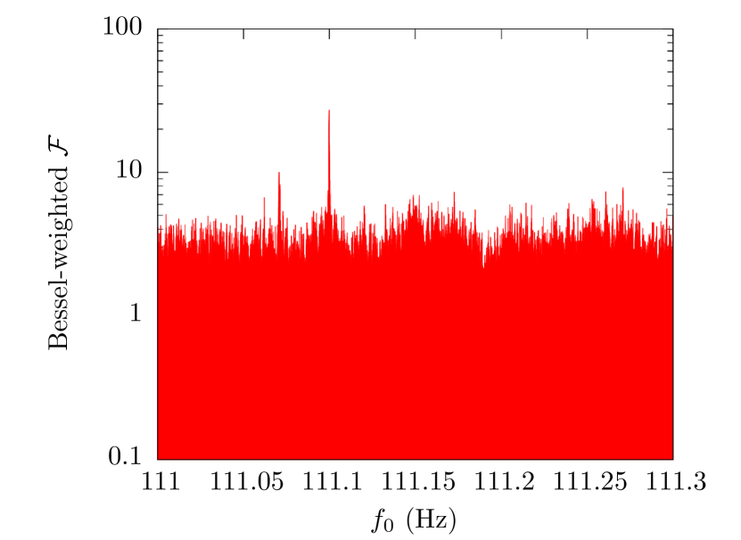
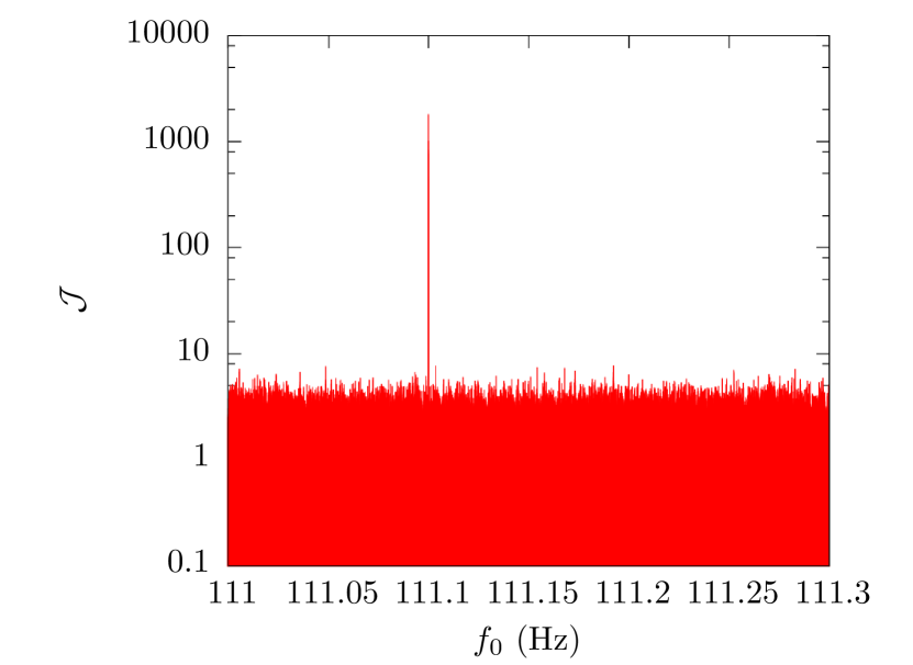
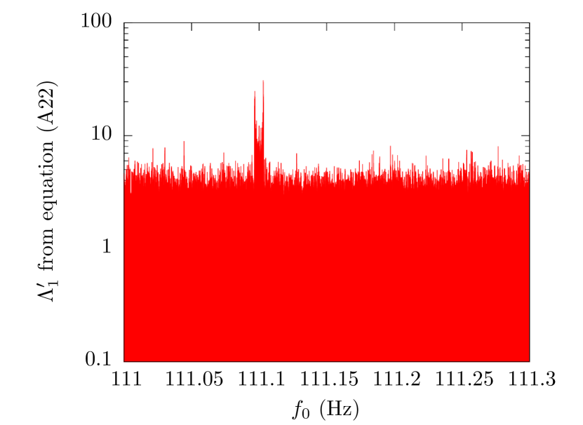
Figure 1 displays the output of four matched filters as a function of $f_{0}$: the $\mathcal{F}$-statistic (Jaranowski et al., 1998), $\mathcal{C}$-statistic Messenger and Woan (2007); Sammut et al. (2014), Bessel-weighted $\mathcal{F}$-statistic (Suvorova et al., 2016), and $\mathcal{J}$-statistic (Section III.2 of this paper). The injected signal is strong, with $h_{0}=8\times 10^{-25}$, making it visible to the eye in all four panels. The matched filters are evaluated for the exact, injected values of $a_{0}$ and $\phi_{a}$, i.e., $f_{0}$ is the only search parameter. In Figure 1(a) we see the distinctive double-horn profile of a binary source in the $\mathcal{F}$-statistic, which arises because a source with inclination angle $\iota\neq 0$ spends more time moving parallel to the line of sight (maximum Doppler shift) than perpendicular to it. (The Fourier transform is the time-weighted frequency histogram.) In Figure 1(b) we see the distinctive onion-dome profile of the $\mathcal{C}$-statistic output. The peak is centred on the value of $f_{0}$ bracketed by the maximum number of significant sidebands. It is broad, because sidebands are summed with equal weights; for weaker but still detectable signals, the peak shrinks and merges into a flat plateau raised above the noise. In Figure 1(c) the onion done transforms into a concave cusp. The peak is sharper and taller than in Figure 1(b), because the Bessel weighting favours the central sidebands, which are intrinsically stronger. In Figure 1(d), corresponding to the $\mathcal{J}$-statistic, the peak is even taller. Essentially zero power falls outside the central bin in the $\mathcal{J}$-statistic; by accounting for the phases $\propto e^{-is\phi_{a}}$ in (26), we avoid power leaking into the shoulders of the peak (cf. Figure 1(c)). The peaks are 11.8, 2.7, 14.6, and 32.6 dB above the noise (that is, the mean for bins containing only noise) in Figures 1(a), 1(b), 1(c), and 1(d) respectively (note logarithmic vertical scale).

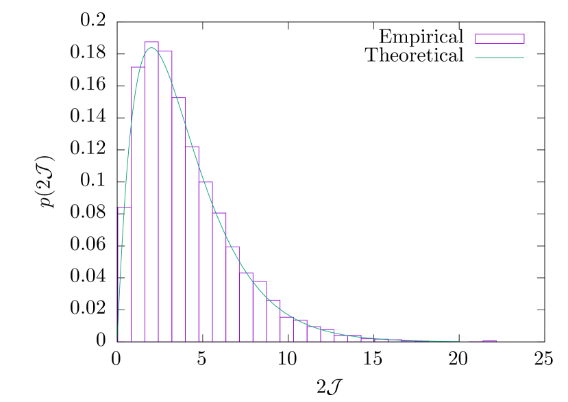
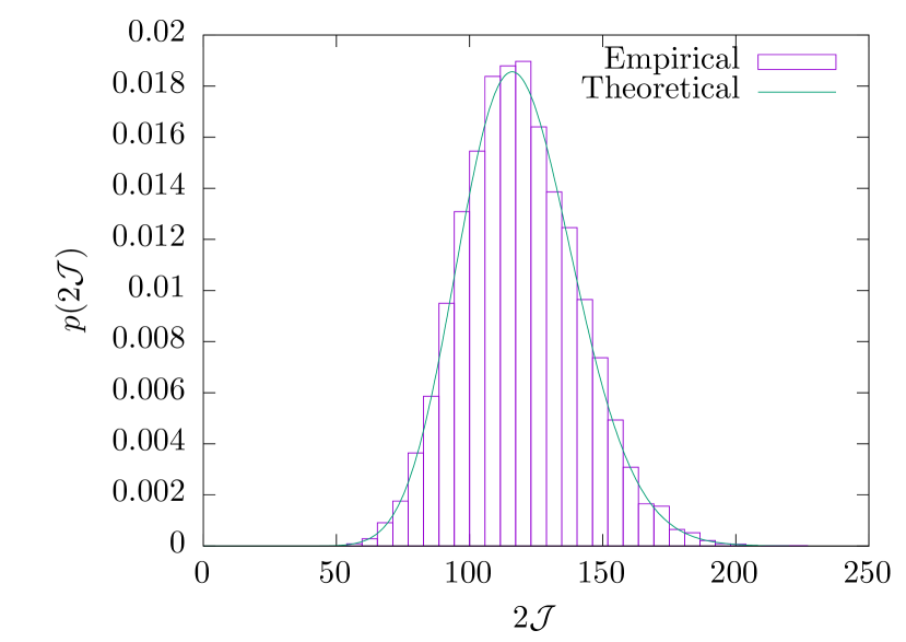
Figure 2 shows the probability density function (PDF) for the $\mathcal{J}$-statistic for pure noise (Figure 2(a)) and noise plus signal (Figure 2(b)). Like the $\mathcal{F}$-statistic (Jaranowski et al., 1998), the $\mathcal{J}$-statistic is distributed as a central chi-squared distribution with four degrees of freedom, $\chi^{2}(4,0)$ for white, Gaussian noise (regardless of the noise amplitude). When a signal is added to the noise, the $\mathcal{J}$-statistic is distributed as a non-central chi-squared distribution with four degrees of freedom, $\chi^{2}(4,\lambda)$. The non-centrality parameter $\lambda$ is related to the amplitude of the signal, the amplitude of the noise and the observation time according to

$$\lambda\propto\frac{h_{0}^{2}T_{\mathrm{obs}}}{S_{h}(f_{0})}.$$ (28)

(a)

(b)

(c)

(d)

Figure 1: Signature of an injected binary signal into the (a) $\mathcal{F}$-statistic (Jaranowski et al., 1998), (b) $\mathcal{C}$-statistic (Sammut et al., 2014), (c) Bessel-weighted $\mathcal{F}$-statistic (Suvorova et al., 2016) and (d) $\mathcal{J}$-statistic. The search frequency $f_{0}$ is plotted on the horizontal axis (units: Hz). All plots are generated from the same synthetic data. The plots are normalised so that the mean of the noise is unity; the mean of the noise appears to be above unity in panels (a) and (d) because each pixel represents many bins. Signal power leaks into orbital sidebands in panels (a)–(c) but is concentrated in a single frequency bin in panel (d). Injection parameters are the same as in Table 1 with $S_{h}(f_{\star})^{1/2}=4\times 10^{-24}\,\mathrm{Hz}^{1/2}$ and $h_{0}=8\times 10^{-25}$.

(a)

(b)

Figure 2: Probability density function of the $\mathcal{J}$-statistic. (a) Noise only. (b) Noise plus injected binary signal with $h_{0}=8\times 10^{-26}$ and other parameters as in Table 1 including $S_{h}(f_{\star})^{1/2}=4\times 10^{-24}\,\mathrm{Hz}^{1/2}$, as in Figure 1. The empirical histograms (purple columns) are generated from $10^{4}$ realisations. The theoretical (green) curves correspond to (2(a)) $\chi^{2}(2\mathcal{J};4,0)$ and (2(b)) $\chi^{2}(2\mathcal{J};4,\lambda)$, with $\lambda=111$ (empirical fit).

IV Synthetic data

IV.1 Injection and search procedure

To assess the effectiveness of the $\mathcal{J}$-statistic, we begin by seeking to detect synthetic signals injected into white, Gaussian noise. To facilitate comparison with previous work, we re-use the trial parameters used by Suvorova et al. (2016) in an identical test of the Bessel-weighted $\mathcal{F}$-statistic. The parameters are quoted in Table 1. Data are generated for $T_{\mathrm{obs}}=370\,\mathrm{d}$, divided into 37 blocks of length $T_{\mathrm{drift}}=10\,\mathrm{d}$. The source frequency $f_{\star}(t)$ is constant within each block and jumps discontinuously by at most one frequency bin ($\Delta f_{\mathrm{drift}}=5.787037\times 10^{-7}\,\mathrm{Hz}$) up or down when passing from one block to the next. We generate data for two interferometers (to facilitate comparison with Section V) using the Makefakedata_v4 tool from the LAL software suite.

Table 1: Injection parameters for the trials on synthetic data in Section IV.

Parameter	Value	Units
$f_{\star}$	$111.1$	Hz
$\dot{f}_{\star}$	$0$	$\mathrm{Hz}\,\mathrm{s}^{-1}$
$\alpha$	$4.2757$	rad
$\delta$	$-0.27297$	rad
$\cos\iota$	$0.71934$	–
$\psi$	$4.08407$	rad
$S_{h}(f_{\star})^{1/2}$	$4\times 10^{-24}$	$\mathrm{Hz}^{-1/2}$
$P$	$68023.7$	s
$a_{0}$	$1.44$	s
$T_{p}$	$1245984672$	s

IV.2 Optimal path

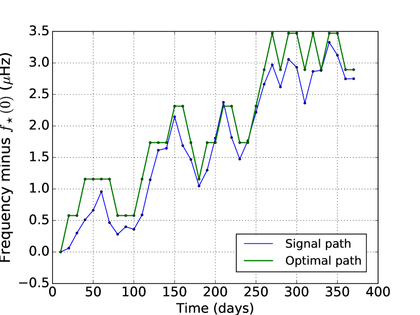
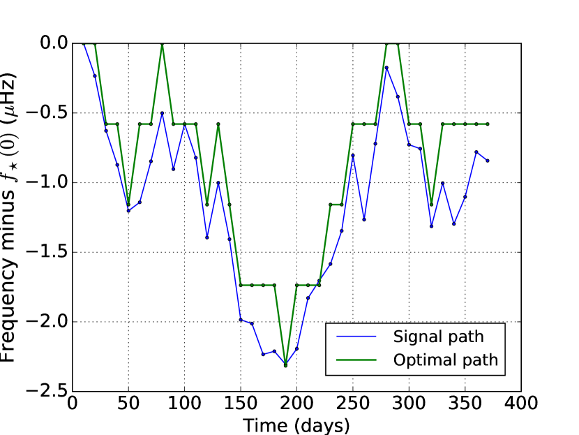
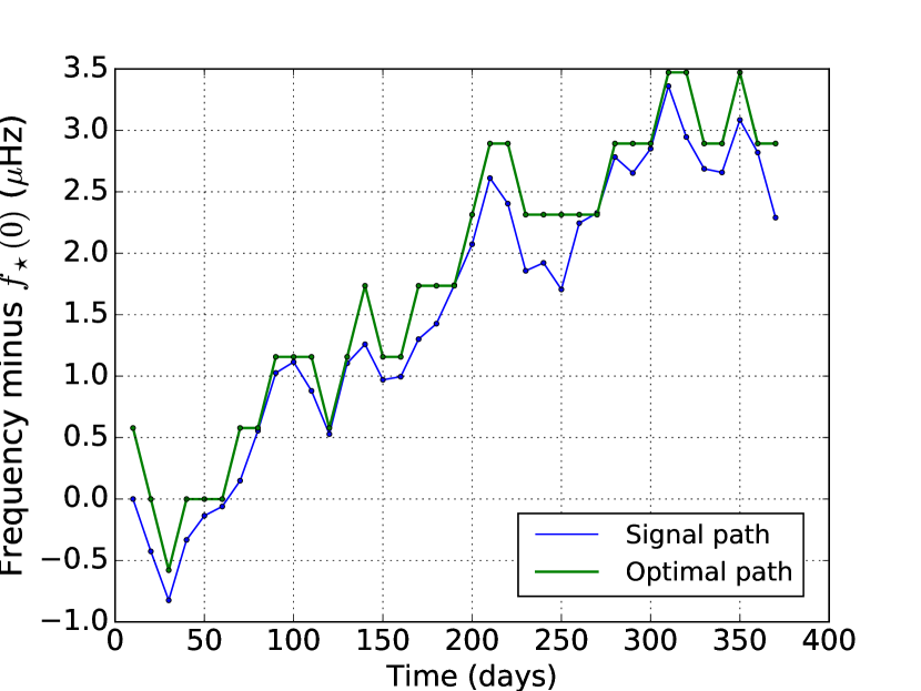
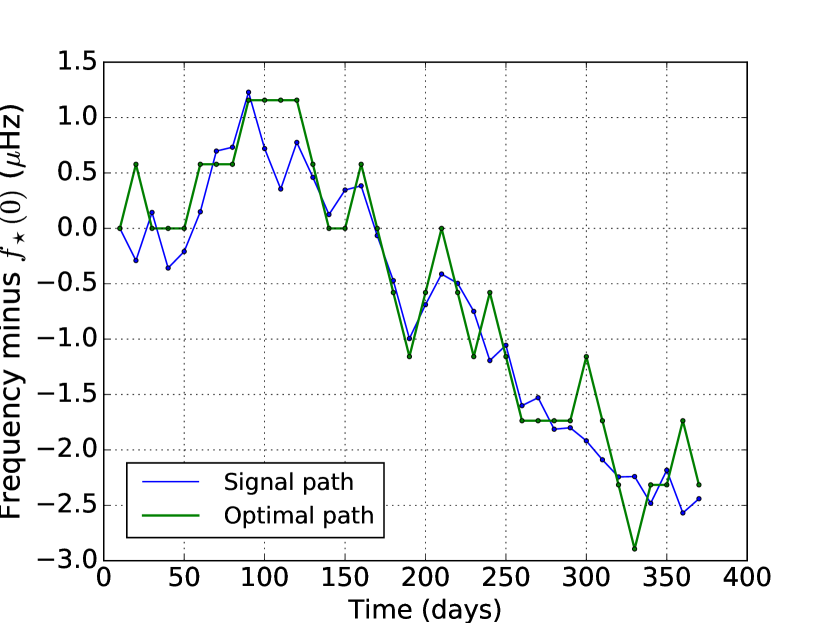
Table 2 lists the outcomes of five trials with $1.5\leq h_{0}/10^{-26}\leq 8$. It shows whether each signal is detected as the optimal Viterbi path and quotes the root-mean-square error $\epsilon_{f_{\star}}$ between the optimal path and $f_{\star}(t)$. We see that the $\mathcal{J}$-statistic is able to recover signals with $h_{0}\geq 2\times 10^{-26}$, consistent with the result in Ref. (Suvorova et al., 2016) for isolated pulsars. The error amounts to $\epsilon_{f_{\star}}\sim 10^{-7}\,\mathrm{Hz}$ for all cases where there is a detection, i.e. as long as the signal can be detected, $\epsilon_{f_{\star}}$ does not worsen, as $h_{0}$ decreases. The error also satisfies $\epsilon_{f_{\star}}\lesssim\Delta f_{\mathrm{drift}}$, i.e., the error is comparable to the frequency resolution of the $\mathcal{J}$-statistic.

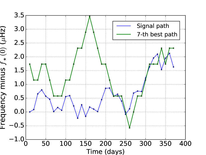
Figure 3 overplots $f_{\star}(t)$ against the paths recovered by the Viterbi algorithm. For signals with $h_{0}\geq 2.0\times 10^{-26}$, the optimal path returned by Viterbi closely matches $f_{\star}(t)$ as noted above. There is a slight mismatch of order one $\mathcal{J}$-statistic frequency bin, because $f_{\star}(t)$ wanders continuously, whereas the HMM transitions between discrete bins. For $h_{0}=1.5\times 10^{-26}$, just below the detection threshold, the optimal path is $0.4\,\mathrm{Hz}$ from the injected path, outside the range plotted in Figure 3(e). Instead Figure 3(e) shows the seventh-ranked Viterbi path, which minimises $\epsilon_{f_{\star}}$. The latter path deviates from $f_{\star}(t)$ in the first half of the data but recovers to converge on $f_{\star}(t)$ towards the end.

The strongest injection in Figure 3(a), with $h_{0}=8.0\times 10^{-26}$, matches the weakest signal detected by the Bessel-weighted $\mathcal{F}$-statistic (Suvorova et al., 2016). With the orbital phase now taken into account, the $\mathcal{J}$-statistic detects the signal without difficulty. Going further, the $\mathcal{J}$-statistic detects injections down to $h_{0}=2.0\times 10^{-26}$. A signal with $h_{0}=2.0\times 10^{-26}$ corresponds to the weakest isolated source (zero orbital motion) detected in Ref. (Suvorova et al., 2016). This suggests that the $\mathcal{J}$-statistic successfully exploits all the orbital phase information to produce a nearly optimal outcome for a semi-coherent algorithm, i.e. it analyses the orbital motion without any degradation in sensitivity relative to an isolated source. The only information it neglects is the phase continuity of the carrier wave at $f_{0}$ from one HMM step to the next. We quantify the optimality of the $\mathcal{J}$-statistic further in Appendix B via an analytic calculation of the Cramér-Rao lower bound.

Table 2: Outcome of Viterbi tracking with the $\mathcal{J}$-statistic in synthetic data containing spin-wandering injections with the parameters in Table 1, $T_{\mathrm{obs}}=370\,\mathrm{d}$, $T_{\mathrm{drift}}=10\,\mathrm{d}$, and wave strain $h_{0}$. The root-mean-square error $\epsilon_{f_{\star}}$ between $f_{\star}(t)$ and the optimal path is quoted in columns 3 and 4.

$h_{0}$ $(10^{-26})$	Detect?	$\epsilon_{f_{\star}}$ (Hz)	$\epsilon_{f_{\star}}/\Delta f_{\mathrm{drift}}$
8.0	✓	$3.54\times 10^{-7}$	$6.12\times 10^{-1}$
5.0	✓	$3.55\times 10^{-7}$	$6.14\times 10^{-1}$
4.0	✓	$3.73\times 10^{-7}$	$6.45\times 10^{-1}$
2.0	✓	$5.80\times 10^{-7}$	$1.00\times 10^{0\phantom{-}}$
1.5	$\times$	$1.91\times 10^{-1}$	$3.31\times 10^{5\phantom{-}}$

(a)

(b)

(c)

(d)

(e)

Figure 3: True $f_{\star}(t)$ (blue curve) and Viterbi path (green curve) for the five injected signals in Table 2 with binary parameters quoted in Table 1. Panels (a)–(d) correspond to $h_{0}/10^{-26}=8,5,4,2$ respectively; a good match between the true and optimal Viterbi paths is obtained in all cases. In panel (e), with $h_{0}/10^{26}=1.5$, the best Viterbi path lies outside the graph’s bounding box; the seventh-best path is plotted instead, which matches $f_{\star}(t)$ best in a root-mean-square sense. The units on the horizontal and vertical axes are days and $\mu\mathrm{Hz}$ respectively.

IV.3 Viterbi score

Once the HMM tracker finds the optimal path, it remains to decide if the path constitutes a detection. We define the Viterbi score $S$, such that the log likelihood of the optimal path exceeds the mean log likelihood of all paths in the relevant sub-band (1 Hz, say, or whatever subdivision makes a broadband search practical) by $S$ standard deviations, viz.

$$S=\frac{\ln\delta_{q^{\star}}(t_{N_{T}})-\mu_{\ln\delta(t_{N_{T}})}}{\sigma_{\ln\delta(t_{N_{T}})}}$$ (29)

with

$$\mu_{\ln\delta(t_{N_{T}})}=N_{Q}^{-1}\sum_{i=1}^{N_{Q}}\ln\delta_{q_{i}}(t_{N_{T}})$$ (30)

and

$$\sigma_{\ln\delta(t_{N_{T}})}^{2}=N_{Q}^{-1}\sum_{i=1}^{N_{Q}}[\ln\delta_{q_{i}}(t_{N_{T}})-\mu_{\ln\delta(t_{N_{T}})}]^{2}.$$ (31)

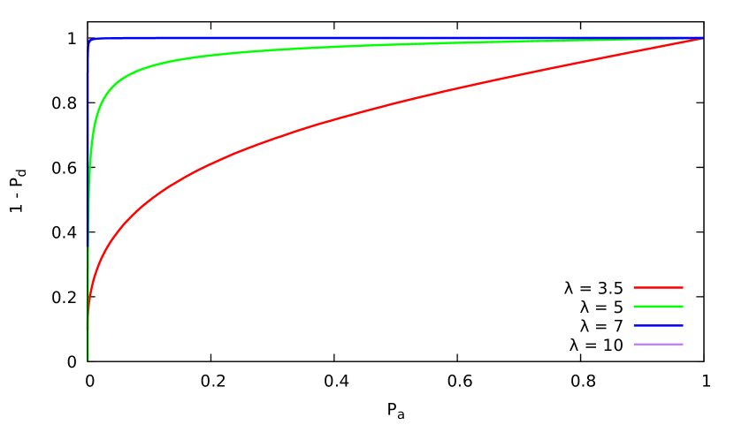
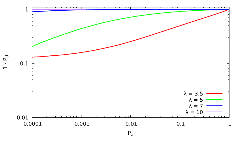
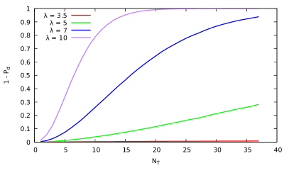
[The symbol $\delta$ is defined in equation (9).] We then establish a threshold $S_{\mathrm{th}}$, and claim a detection for $S>S_{\mathrm{th}}$. The threshold determines the false alarm probability $P_{\mathrm{a}}$. Selecting a desired false dismissal probability, $P_{\mathrm{d}}$, then determines the weakest signal we can reliably detect.

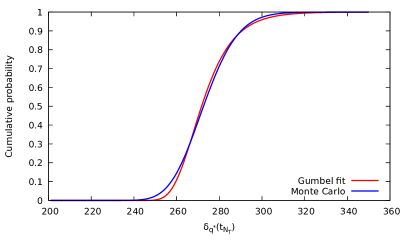
Appendix C discusses in detail the PDF of the terminal Viterbi probabilities $\delta_{q_{i}}(t_{N_{T}})$ in (9). To the authors’ knowledge, an analytic formula for the PDF does not exist in the literature; the calculation is rendered difficult by the correlations between Viterbi paths and the nonlinear maximisation step in the algorithm. Appendix C presents an empirical fit to the associated cumulative distribution function in the form of a Gumbel law, motivated by asymptotic results from extreme value theory (Sornette, 2004). The two parameters of the fit (denoted by $a$ and $b$ in Appendix C) are tabulated as functions of $N_{Q}$ and $N_{T}$ in Table 7 in the appendix.

Table 3 presents $P_{\mathrm{a}}$ as a function of $S_{\mathrm{th}}$ for six convenient, representative, integer thresholds. For the searches described in this paper, we choose $S_{\mathrm{th}}=7$, which corresponds to $P_{\mathrm{a}}=7.1\times 10^{-3}$, close to the false alarm probability of $1\%$ per cent appearing commonly in the literature. The choice $S_{\mathrm{th}}=7$ also matches what was done in Ref. (Suvorova et al., 2016), for ease of comparison.

Table 3: False alarm probability $P_{\mathrm{a}}$ versus Viterbi score threshold $S_{\mathrm{th}}$ in equation (29).

$S_{\mathrm{th}}$	$P_{\mathrm{a}}$
5	$9.4\times 10^{-2}$
6	$2.6\times 10^{-2}$
7	$7.1\times 10^{-3}$
8	$2.0\times 10^{-3}$
9	$5.0\times 10^{-4}$
10	$1.5\times 10^{-4}$

IV.4 Sensitivity to orbital parameters

Electromagnetic observations of LMXBs play an important role in narrowing down the range of possible values of the projected semimajor axis $a_{0}$ and reference orbital phase $\phi_{a}$ (Premachandra et al., 2016; Galloway et al., 2014). Typically, however, the range is wider than the resolution of the $\mathcal{J}$-statistic–based HMM, and a search over multiple templates within the range is still required.

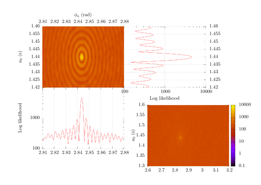
Figure 4 quantifies the resolution of the $\mathcal{J}$-statistic–based HMM in $a_{0}$ and $\phi_{a}$ to help fix the template spacing. The figure is drawn for a synthetic signal with $h_{0}=8\times 10^{-26}$, with parameters as in Table 1. It plots log likelihood for $1.3\leq a_{0}/\mathrm{s}\leq 1.6$, $2.6\leq\phi_{a}/\mathrm{rad}\leq 3.2$, and $N_{T}=37$. All other parameters, including the search frequency $f_{0}=f_{\star}$, are held fixed at their injected values. The grid resolution is $1\times 10^{-4}\,\mathrm{s}$ for $a_{0}$ and $1.5259\times 10^{-5}\,\mathrm{rad}$ for $\phi_{a}$. The figure shows a clear peak at the injected values of $a_{0}$ and $\phi_{a}$. The peak is surrounded by rings (particularly visible in the zoomed upper-left panel), which arise for two reasons: (i) the decision in equation (26) to sum a finite number of sidebands, which introduces a $\operatorname*{sinc}$-function envelope as $a_{0}$ changes, and (ii) the finite observation time, which introduces a $\operatorname*{sinc}$-function envelope, as $\phi_{a}$ changes. There are no false peaks away from the injected values.

The $\mathcal{J}$-statistic is sensitive to errors in $a_{0}$. For example, a 10% error in the measured value of $a_{0}$ causes a drop of two orders of magnitude in the log likelihood, while the $\mathcal{C}$-statistic sees a 10% reduction in detection probability for the same situation (see Figure 4 in Ref. (Sammut et al., 2014)). The $a_{0}$ range covered in Figure 4 is comparable to the uncertainty in the electromagnetic measurement of $a_{0}$ at the time Stage I of the Sco X-1 MDC was run (Messenger et al., 2015; Steeghs and Casares, 2002). Since then, the uncertainty has increased to $0.36\,\mathrm{s}$–$3.25\,\mathrm{s}$ (Z. Wang et al., private communication). The computational cost scales linearly with the range of $a_{0}$.

Figure 4: Log likelihood as a function of reference orbital phase $\phi_{a}$ and projected semi-major axis $a_{0}$ for a search with $N_{T}=37$ using two interferometers on synthetic data, for the parameters in Table 1 with $h_{0}=8\times 10^{-26}$. (Top left.) Contour plot of log likelihood on the $\phi_{a}$ - $a_{0}$ plane near the injection. The colour scale shows the log likelihood and is defined by the colour bar in the bottom right panel. (Top right.) Cross-section of log likelihood versus $a_{0}$ (units: s). The cross section is at $\phi_{a}=0.6080\,\mathrm{rad}$, chosen to pass through the peak. (Bottom left.) Cross-section of log likelihood versus $\phi_{a}$ (units: rad). The cross section is at $a_{0}=1.3138\,\mathrm{s}$, again chosen to pass through the peak. (Bottom right.) Contour plot showing the entire parameter range searched. No spurious detections are found away from the injection parameters.

V Sco X-1 mock data challenge: A “realistic” example

The next stage in validating the $\mathcal{J}$-statistic–based HMM is to engage in Stage I (version 6) of the Sco X-1 MDC (Messenger et al., 2015). The MDC is based on a mock observational dataset intended to simulate the noise level and duty cycle of Advanced LIGO. Stage I of the MDC comprises 50 Sco X-1–type signals without spin wandering injected into Gaussian noise. (Messenger et al., 2015) Stage II of the MDC is currently being prepared and is planned to include spin wandering. The MDC establishes a standard to compare the $\mathcal{J}$-statistic HMM tracker against the Bessel-weighted $\mathcal{F}$-statistic Suvorova et al. (2016), CrossCorr (Dhurandhar et al., 2008; Chung et al., 2011; Whelan et al., 2015; Sun et al., 2016), TwoSpect (Aasi et al., 2014a; Goetz and Riles, 2011; Meadors et al., 2016), Radiometer (Abadie et al., 2011), Sideband (Aasi et al., 2015a; Sammut et al., 2014; Messenger and Woan, 2007) and Polynomial (van der Putten et al., 2010) pipelines.

The parameters of the 50 Stage I MDC injections are listed in Table III of Ref. (Messenger et al., 2015). Originally, these 50 injections were “closed”, i.e. their parameters were kept secret to enable a blind comparison. The TwoSpect, Radiometer, Sideband and Polynomial pipelines performed the test under closed conditions as reported in Ref. (Messenger et al., 2015), while CrossCorr and the Bessel-weighted $\mathcal{F}$-statistic (Suvorova et al., 2016) participated after the release of the parameters under self-blinded conditions, as we propose to do here. Participants in the original tests were asked to assume, that the injections experience spin wandering (although they do not), with the Sideband search being restricted to $T_{\mathrm{obs}}=10\,\mathrm{d}$ as a result (Messenger et al., 2015). We use the transition matrix (3) to replicate this mode of operation.

The orbital period $P$ of Sco X-1 is measured to $\pm 0.04\,\mathrm{s}$ (Galloway et al., 2014). The error in sideband frequency, for all $M$ sidebands, must be less than one $\mathcal{J}$-statistic frequency bin, which limits the allowed uncertainty in $P$ to $|\Delta P|\leq P^{2}/(MT_{\mathrm{drift}})\leq 0.2\,\mathrm{s}$. This suggests that searching over $P$ is unnecessary. For the search described in this section, we assume $P=68023.70\,\mathrm{s}$ for all injections (Galloway et al., 2014) (cf. Table II in Ref. (Messenger et al., 2015)).

We divide the year-long dataset, starting at GPS time $1\,230\,338\,490$, into $N_{T}=37$ blocks with $T_{\mathrm{drift}}=10\,\mathrm{d}$. Data from two simulated interferometers (H1 and L1) are used in the analysis below.

V.1 Single block: $N_{T}=1$

The first step is to ask how many injections are detected using the first block only ($N_{T}=1$). We find that the answer is 43 out of 50. The exceptions are those with index 41, 48, 57, 64, 72, 73 and 90. By way of comparison, the Bessel-weighted $\mathcal{F}$-statistic with $N_{T}=1$ and two interferometers detects only 12 signals (Suvorova et al., 2016), and the $\mathcal{C}$-statistic with $N_{T}=1$ and three interferometers detects 16 signals (Messenger et al., 2015).

Detailed test results are presented in Table 4. The table lists the injection parameters ($f_{\star}$, $a_{0}$, $\phi_{a}$, $h_{0}$) as well as the absolute (as opposed to relative) errors $\epsilon_{f_{\star}}$, $\epsilon_{a_{0}}$ and $\epsilon_{\phi_{a}}$ in the recovered values for $f_{\star}$, $a_{0}$ and $\phi_{a}$ respectively. For $a_{0}$ and $\phi_{a}$, the search returns single grid values, so $\epsilon_{a_{0}}$ and $\epsilon_{\phi_{a}}$ are defined as the signed difference between the injected and recovered values. For $f_{\star}$, which wanders in general, we define $\epsilon_{f_{\star}}$ as the root-mean-square error between the injected and optimal paths for however many blocks are needed to achieve a detection, in preparation for the analysis in Section V.2 with $N_{T}>1$.

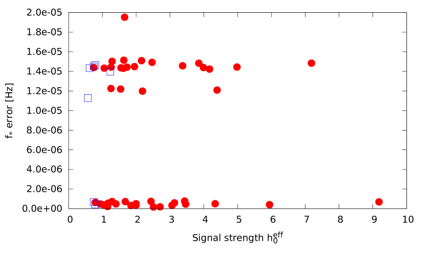
For most signals, the error in $a_{0}$ and $\phi_{a}$ is smaller than the bin size for those parameters ($1\times 10^{-4}\,\mathrm{s}$ for $a_{0}$ and $1.5259\times 10^{-5}\,\mathrm{rad}$ for $\phi_{a}$), so the error is the difference between the bin boundary and the injection parameter. The log likelihood peaks sharply, as the estimate of $\phi_{a}$ improves, so it may be possible to improve the sensitivity somewhat by estimating $\phi_{a}$ more precisely. We defer to future work the task of determining the optimal template spacing for a given mismatch using the parameter space metrics derived in Ref. (Leaci and Prix, 2015). For 13 injections, the RMS error between the optimal and injected paths is less than the $\mathcal{J}$-statistic frequency bin width, $\Delta f_{\mathrm{drift}}=5.8\times 10^{-7}\,\mathrm{Hz}$, and seven more have $1.0\Delta f_{\mathrm{drift}}\leq\epsilon_{f_{s}tar}\leq 1.5\Delta f_{\mathrm{drift}}$. The remaining 23 injections are detected with frequency error $19\Delta f_{\mathrm{drift}}<\epsilon_{f_{\star}}<34\Delta f_{\mathrm{drift}}$. The distance (in frequency space) between this group and the group with error less than $1.5\Delta f_{\mathrm{drift}}$ corresponds roughly to the frequency separation between sidebands.

The characteristic wave strain $h_{0}$ influences detectability, in conjunction with the source inclination angle $\iota$, which enters the plus and cross polarisations differently. A popular, approximate proxy for signal strength, given by equation (19) in Ref. (Messenger et al., 2015), is the effective characteristic wave strain

$$h^{\mathrm{eff}}_{0}=h_{0}2^{-1/2}\{[(1+\cos^{2}\iota)/2]^{2}+\cos^{2}\iota\}^{1/2}.$$ (32)

To test if $h^{\mathrm{eff}}_{0}$ captures faithfully the joint dependence of detectability on $h_{0}$ and $\iota$, we generate synthetic signals for $0\leq\cos\iota\leq 1$ and $0\leq\psi\leq 2\pi$, while holding $h^{\mathrm{eff}}_{0}$ constant (that is, with different values of $h_{0}$ for each $\iota$ value) and calculate the $\mathcal{J}$-statistic. If $h^{\mathrm{eff}}_{0}$ is a perfect proxy, we expect the same $\mathcal{J}$-statistic output for all $\iota$. The results of 100 Monte-Carlo realisations per $(\cos\iota,\psi)$ pair are plotted in Figure 5. Indeed the $\mathcal{J}$-statistic score is roughly constant, showing no discernible pattern across the full parameter space, and fluctuating by $\leq 12\%$.

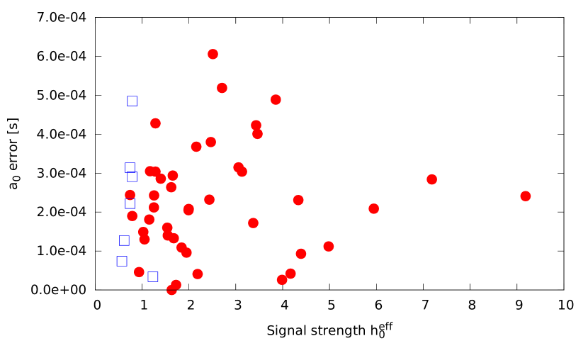
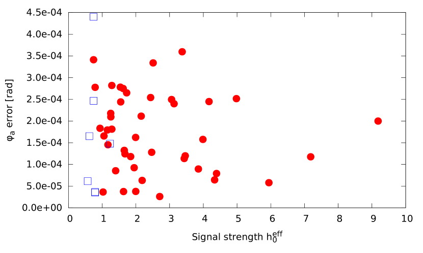
Figure 6 summarises the error estimates in Table 4. It displays $\epsilon_{f_{\star}}$, $\epsilon_{a_{0}}$ and $\epsilon_{\phi_{a}}$ plotted against $h^{\mathrm{eff}}_{0}$. The vertical “step” in $\epsilon_{f_{\star}}$ visible in Figure 6(a) corresponds to the sideband separation $P^{-1}$. In Figures 6(b) and 6(c), $\epsilon_{a_{0}}$ and $\epsilon_{\phi_{a}}$ are comparable to the grid resolution, with all 50 injections having errors less than seven ($\epsilon_{a_{0}}$) or five ($\epsilon_{\phi_{a}}$) search bins. There is no apparent correlation between the errors and $h^{\mathrm{eff}}_{0}$ amongst the injections that are detected successfully.

Figure 5: Log likelihood (for $N_{T}=1$) versus orientation angles $\cos\iota$ and $\psi$, holding $h^{\mathrm{eff}}_{0}=8\times 10^{-26}$ fixed and all other parameters as in Table 1. Each grid cell is an average over $10^{2}$ noise realisations.

(a)

(b)

(c)

Figure 6: Accuracy of the $\mathcal{J}$-statistic–based HMM applied to Stage I of the Sco X-1 MDC versus effective characteristic wave strain $h^{\mathrm{eff}}_{0}$. (a) Root-mean-square error in $f_{\star}$ (Hz). (b) Absolute unsigned error in $a_{0}$ (in s). (c) Absolute unsigned error in $\phi_{a}$ (in rad). The cluster in (a) at $\epsilon_{f_{\star}}\approx 1.4\times 10^{-5}\,\mathrm{Hz}$ corresponds to the orbital sideband separation $P^{-1}$. All 50 MDC injections are shown: 43 are detected with $N_{T}=1$ (filled red circles; see section V.1), while seven require $1<N_{T}\leq 37$ (open blue squares; see section V.2).

V.2 Multiple blocks, $1<N_{T}\leq 37$

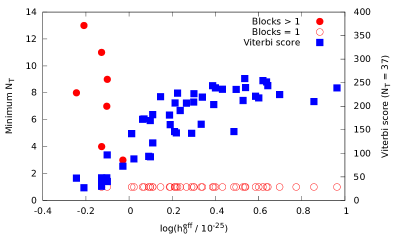
For the seven out of 50 injections that are not detected with $N_{T}=1$, we do HMM tracking for $T_{\mathrm{drift}}=10\,\mathrm{d}$ and $1<N_{T}\leq 37$. The search parameters and prior are the same as in Section V.1. We successfully detect all seven remaining injections, with $N_{T}=3$ for injection 73, $N_{T}=13$ for injection $90$, and the others in between, as in Table 5.

Figure 7 summarises the results in Tables 4 and 5. It plots all 50 injections twice against $h^{\mathrm{eff}}_{0}$. The red circles (left axis) indicate the minimum $N_{T}$ required to achieve a detection. Most injections are detected in a single block (open red circles). The seven injections requiring multiple blocks (filled red circles) are all weak signals, along the left-hand border of the plot. The blue squares (right axis) show the Viterbi score $S$ after processing the full year of data, even if the signal is detected with $N_{T}<37$. There is a positive correlation between $S$ and $h^{\mathrm{eff}}_{0}$, with $S\propto h^{\mathrm{eff}}_{0}$ roughly for $S\lesssim 2.6\times 10^{2}$. The Viterbi score for injection 66 ($S=522$) lies outside the range of the graph, due to a lucky coincidence of a relatively strong signal and a $\phi_{a}$ value that happens to lie close to the search grid.

Figure 7: Minimum number of 10-d data blocks $N_{T}$ for a detection (left axis; red circles, filled for $N_{T}>1$, open for $N_{T}=1$) and Viterbi score $S$ with $N_{T}=37$ (right axis; blue squares) versus the logarithm of the effective characteristic wave strain for 50 injections in Stage 1 of the Sco X-1 MDC.

Table 4: Results of $\mathcal{J}$-statistic HMM tracking of the 50 closed signals in Stage I (version 6) of the Sco X-1 MDC, ordered by ascending injection frequency $f_{\star}$. The index is copied from Ref. (Messenger et al., 2015). Signal strength is quantified by $h_{0}$ (traditional gravitational wave strain in Ref. (Jaranowski et al., 1998; Messenger et al., 2015)) and $h^{\mathrm{eff}}_{0}$ (Ref. (Messenger et al., 2015)). The recovered orbital parameters $a_{0}$ and $\phi_{a}$ and their signed, absolute errors appear in columns six to nine.

Index	$h_{0}$	$h^{\mathrm{eff}}_{0}$	$f_{\star}$	$\epsilon_{f_{\star}}$	$a_{0}$	$\epsilon_{a_{0}}$	$\phi_{a}$	$\epsilon_{\phi_{a}}$
	($10^{-25}$)	($10^{-25}$)	(Hz)	(Hz)	(s)	(s)	(rad)	(rad)
1	4.160101	2.706	54.498391348174	1.853E-07	1.379519	5.190E-04	0.564832303	-2.606E-05
2	4.044048	2.511	64.411966012332	1.681E-07	1.764606	6.060E-04	0.572064312	-3.339E-04
3	3.565197	3.463	73.795580913582	4.603E-07	1.534599	-4.010E-04	0.585084391	1.198E-04
5	1.250212	1.154	93.909518008164	2.244E-07	1.520181	1.810E-04	0.633165725	-1.794E-04
11	3.089380	1.399	154.916883586097	4.866E-07	1.392286	2.860E-04	0.576082666	-8.545E-05
14	2.044140	1.286	183.974917468730	7.248E-07	1.509696	-3.040E-04	0.577142828	-2.819E-04
15	11.763777	4.169	191.580343388804	1.424E-05	1.518142	4.200E-05	0.599799259	-2.449E-04
17	3.473418	1.253	213.232194220000	1.225E-05	1.310212	2.120E-04	0.578899085	2.177E-04
19	6.030529	2.437	233.432565653291	7.465E-07	1.231232	2.320E-04	0.596020206	-2.541E-04
20	9.709634	3.434	244.534697522529	7.748E-07	1.284423	4.230E-04	0.617523371	-1.137E-04
21	1.815111	0.792	254.415047846878	6.374E-07	1.072190	1.900E-04	0.595996707	-2.776E-04
23	2.968392	1.677	271.739907539784	7.173E-07	1.442867	-1.330E-04	0.598663241	-1.243E-04
26	1.419173	1.172	300.590450155009	5.630E-07	1.258695	-3.050E-04	0.610242598	1.453E-04
29	4.274554	3.131	330.590357652653	5.968E-07	1.330696	-3.040E-04	0.580326474	-2.398E-04
32	10.037770	4.391	362.990820993568	1.209E-05	1.611093	9.300E-05	0.573105599	7.911E-05
35	16.401523	9.183	394.685589797695	6.921E-07	1.313759	-2.410E-04	0.608012394	-1.999E-04
36	3.864262	1.539	402.721233789014	1.219E-05	1.254840	-1.600E-04	0.602207114	2.780E-04
41	1.562041	0.746	454.865249156175	6.744E-07	1.465778	-2.220E-04	0.605945666	2.466E-04
44	2.237079	1.996	483.519617972096	5.065E-07	1.552208	2.080E-04	0.590657162	3.774E-05
47	4.883365	1.992	514.568399601819	3.425E-07	1.140205	2.050E-04	0.563763897	1.622E-04
48	1.813016	0.745	520.177348201609	1.451E-05	1.336686	-3.140E-04	0.563161604	-4.401E-04
50	1.092771	1.027	542.952477491471	4.038E-07	1.119149	1.490E-04	0.542275328	3.644E-05
51	9.146386	3.372	552.120598886904	1.457E-05	1.327828	-1.720E-04	0.573295251	-3.596E-04
52	2.785731	1.550	560.755048768919	1.436E-05	1.792140	1.400E-04	0.594773666	-2.440E-04
54	1.517530	1.256	593.663030872532	1.443E-05	1.612757	-2.430E-04	0.569675332	-2.095E-04
57	1.576918	0.788	622.605388362863	4.347E-07	1.513291	2.910E-04	0.608877237	3.658E-05
58	3.416297	1.287	641.491604906276	1.503E-05	1.584428	4.280E-04	0.602738791	1.813E-04
59	8.834794	4.981	650.344230698489	1.444E-05	1.677112	1.120E-04	0.550155435	-2.516E-04
60	2.960648	2.467	664.611446618250	1.492E-05	1.582620	-3.800E-04	0.568756259	1.280E-04
61	6.064238	2.158	674.711567789201	1.509E-05	1.499368	3.680E-04	0.626850596	-2.113E-04
62	10.737497	3.853	683.436210983289	1.483E-05	1.269511	-4.890E-04	0.585682431	8.954E-05
63	1.119028	0.745	690.534687981171	1.440E-05	1.518244	2.440E-04	0.587764962	-3.412E-04
64	1.599528	0.570	700.866836291234	1.129E-05	1.399926	-7.400E-05	0.571080095	-6.145E-05
65	8.473643	4.334	713.378001688688	5.023E-07	1.145769	-2.310E-04	3.981714377	6.434E-05
66	9.312048	5.944	731.006818153273	4.061E-07	1.321791	-2.090E-04	3.937174208	-5.789E-05
67	4.579697	1.623	744.255707971300	1.432E-05	1.677736	-2.640E-04	0.619168642	2.749E-04
68	3.695848	1.844	754.435956775916	3.240E-07	1.413891	-1.090E-04	0.577934937	-1.181E-04
69	2.889282	1.053	761.538797037770	1.433E-05	1.626130	1.300E-04	0.642604270	-1.656E-04
71	2.922576	1.232	804.231717847467	1.398E-05	1.652034	3.400E-05	0.614347724	-1.478E-04
72	1.248093	0.792	812.280741438401	1.466E-05	1.196485	4.850E-04	0.612575356	-3.521E-05
73	2.443983	0.936	824.988633484129	4.802E-07	1.417154	-4.600E-05	0.545563765	1.833E-04
75	7.678400	3.987	862.398935287248	1.440E-05	1.567026	2.600E-05	3.958458316	1.576E-04
76	3.260143	1.725	882.747979842807	1.443E-05	1.462487	-1.300E-05	0.648061399	2.650E-04
79	4.680848	1.656	931.006000308958	1.953E-05	1.491706	-2.940E-04	0.598919953	1.324E-04
83	5.924668	2.186	1081.398956458276	1.198E-05	1.198541	4.100E-05	0.598724345	-6.321E-05
84	11.608892	7.184	1100.906018344283	1.484E-05	1.589716	-2.840E-04	0.609351448	-1.176E-04
85	4.552730	1.633	1111.576831848269	1.514E-05	1.344790	0.000E+00	0.623329562	3.758E-05
90	0.684002	0.618	1193.191890630547	1.433E-05	1.575127	1.270E-04	0.636321462	-1.652E-04
95	4.293322	3.059	1324.567365220908	3.271E-07	1.591685	-3.150E-04	0.587727432	2.496E-04
98	5.404060	1.948	1372.042154535880	1.449E-05	1.315096	9.600E-05	0.640164126	-9.243E-05

Table 5: Minimum number of data blocks $N_{T}$ required to detect the seven MDC injections that cannot be detected with $N_{T}=1$. Indices refer to Table 4. A detection is claimed when the Viterbi score exceeds the mean by at least seven standard deviations ($S>7$).

Index	Blocks
41	4
48	11
57	7
64	8
72	9
73	3
90	13

VI Conclusion

In this paper, we extend the HMM scheme for tracking continuous-wave gravitational radiation from a neutron star undergoing spin wandering in an LMXB described in Ref. (Suvorova et al., 2016). The new scheme tracks the orbital phase of the source by using a frequency-domain matched filter, termed the $\mathcal{J}$-statistic, to compute the emission probabilities at each HMM step. The $\mathcal{J}$-statistic sums the $\mathcal{F}$-statistic power in orbital sidebands coherently by weighting each sideband by a suitable Bessel amplitude and Fourier phase. Monte-Carlo simulations in Gaussian noise with $S_{h}(f_{\star})^{1/2}=4\times 10^{-24}\,\mathrm{Hz}^{-1/2}$ show that the $\mathcal{J}$-statistic HMM successfully detects spin-wandering injections with wave strain $h_{0}\gtrsim 2\times 10^{-26}$ with two interferometers. This equals the sensitivity achieved in Ref. (Suvorova et al., 2016) for isolated neutron stars; the $\mathcal{J}$-statistic succeeds in marshalling all the signal power in orbital sidebands into a single frequency bin with essentially zero leakage. Even better sensitivity will be achieved when combining three interferometers.

When competing in self-blinded mode in Stage I of the Sco X-1 MDC, the $\mathcal{J}$-statistic HMM detects all 50 signals, 43 of them using a single HMM step ($10\,\mathrm{d}$ of data). It estimates $f_{\star}$, $a_{0}$ and $\phi_{a}$ to accuracies of $\epsilon_{f_{\star}}<2\times 10^{-5}\,\mathrm{Hz}$, $\epsilon_{a_{0}}<6\times 10^{-5}\,\mathrm{s}$, $\epsilon_{\phi_{a}}<4\times 10^{-4}\,\mathrm{rad}$ respectively. By comparison, the CrossCorr, Bessel-weighted $\mathcal{F}$-statistic HMM, TwoSpect, Radiometer, Sideband and Polynomial methods found 50, 41, 34, 28, 16 and 7 out of 50 signals, respectively. The accuracy of $f_{\star}$ estimation by the $\mathcal{J}$-statistic HMM is roughly as good as the most accurate existing algorithms (CrossCorr, Bessel-weighted HMM, TwoSpect). The same is true for its accuracy of $a_{0}$ estimation. (Radiometer and Polynomial do not estimate $a_{0}$.) A comparison of the performance metrics for the seven algorithms listed above is presented in Table 6. The $\mathcal{J}$-statistic HMM is the only scheme to be tested formally on spin-wandering data, as reported here, although this will change when Stage II of the Sco X-1 MDC is completed. We emphasise that several of the algorithms in Table 6 have undergone substantial refinement, since Ref. (Messenger et al., 2015) was published, e.g. the tuned TwoSpect method (Meadors et al., 2016). When performance data are published for the refined algorithms, some of the entries in Table 6 will require updating.

Although this paper focuses on spin wandering in LMXBs, the same methods are likely to prove helpful when searching for isolated, nonaccreting neutron stars as well. Radio timing experiments reveal that spin wandering is endemic in rotation-powered pulsars, where it goes by the name of ‘timing noise’ (Hobbs et al., 2010; Shannon and Cordes, 2010). Timing noise exhibits a red spectrum and is autocorrelated on time-scales ranging from days to years (Cordes and Helfand, 1980; Price et al., 2012). Its physical origin is still debated, but it is generically attributed to fluctuations in the structure of the magnetosphere and/or superfluid interior (Alpar et al., 1986; Cheng, 1987; Jones, 1990; Hobbs et al., 2010; Lyne et al., 2010; Melatos and Link, 2014). Until now, continuous-wave searches have handled timing noise in various ways. All-sky searches for periodic signals from isolated neutron stars in the LIGO (S5 and S6) and Virgo (VSR1 to VSR4) data sets, using various algorithms (e.g., loosely coherent, Hough, $\mathcal{F}$-statistic), typically consider a range of spin-down rates (Aasi et al., 2013a, 2016a, 2014a; Walsh et al., 2016). For these experiments, spin wandering effectively limits the maximum observation time, before the phase model loses coherence with the source. The same applies to directed $\mathcal{F}$-statistic and hierarchical searches pointed at young supernova remnants and the Galactic centre respectively (Aasi et al., 2013b, 2016b; Abadie et al., 2010). Coherent narrowband searches for objects like the Crab and Vela pulsars are guided by radio pulsar timing ephemerides, so in principle the timing noise is tracked electromagnetically (Aasi et al., 2016a; Abbott et al., 2008; Aasi et al., 2014b, 2013a; Abadie et al., 2011; Abbott et al., 2010). Even so there is no guarantee that the gravitational-wave-emitting quadrupole is locked to the stellar crust and magnetic field and hence the radio emission; a lag may exist between the two components and it may fluctuate stochastically (Warszawski and Melatos, 2013; Melatos and Link, 2014; Melatos et al., 2015). Coherent narrowband searches usually safeguard against this eventuality by scanning a band of frequency centred on the radio ephemeris, typically $\sim\pm 10^{-2}\,\mathrm{Hz}$ wide, without explicitly testing all possible frequency wandering paths within the band, e.g., (Aasi et al., 2015b). Ashton et al. (2015) quantified the loss of sensitivity caused by timing noise in ephemeris-guided narrowband searches, calculating the template mismatch as a function of the total observation time. We will investigate the performance of HMM frequency tracking in these contexts in future work.

Table 6: Comparison between the $\mathcal{J}$-statistic HMM (Viterbi 2.0) and other algorithms that participated in Stage I of the Sco X-1 MDC. Viterbi 1.0 refers to the Bessel-weighted $\mathcal{F}$-statistic combined with the Viterbi HMM solver in Ref. (Suvorova et al., 2016). The table does not include unpublished performance improvements to several algorithms listed.

	Viterbi 2.0	CrossCorr	Viterbi 1.0	TwoSpect	Radiometer	Sideband	Polynomial
Hit rate (out of 50)	50	50	41	34	28	16	7
Best $h_{0}$ $(10^{-25})$	0.684	0.684	1.093	1.250	2.237	3.565	7.678
Best $h_{0}/\sqrt{f_{\star}}$ ($10^{-25}\,\mathrm{Hz}^{-1/2}$)	0.020	0.020	0.047	0.082	0.102	0.235	0.261
Typical $\epsilon_{f_{\star}}$ (Hz)	$10^{-5}$	$10^{-5}$	$10^{-5}$	$10^{-4}$	$10^{-1}$	$10^{-2}$	$10^{-2}$
Typical $\epsilon_{a_{0}}$ (s)	$10^{-4}$	$10^{-4}$	$10^{-4}$	$10^{-2}$	—	—	—
Typical run time (CPU-hr)	$10^{5}$	$10^{6}$	$10^{3}$	$10^{5}$	$10^{3}$	$10^{3}$	$10^{8}$

VII Acknowledgements

We thank the LIGO Scientific Collaboration Continuous Wave Working Group for informative discussions. The synthetic data for Stage I of the Sco X-1 MDC were prepared primarily by Chris Messenger with the assistance of members of the MDC team. (Messenger et al., 2015) P. Clearwater is supported by a Melbourne Research Scholarship and a CSIRO Office of the Chief Executive Postgraduate PhD Scholarship in Zettabyte Data Management. L. Sun is supported by an Australian Postgraduate Award. This work was supported by the Multi-modal Australian ScienceS Imaging and Visualisation Environment (MASSIVE), by Australian Research Council (ARC) Discovery Project DP110103347, ARC Centre of Excellence CE170100004 and by the U.S. Air Force Office of Scientific Research under Grant No. FA9550-12-1-0418.

(a)

(b)

Figure 8: Signature of an injected binary signal in (a) the Bessel-weighted $\mathcal{F}$-statistic, described in Ref. (Suvorova et al., 2016) and (b) the quasi-maximum likelihood estimator, defined by (54). As in Figure 1, the plots are normalised such that the mean of the noise is unity. Parameters: as in Table 1, with $h_{0}=8\times 10^{-25}$.

Appendix A Quasi–maximum-likelihood generalisations of the $\mathcal{F}$-statistic for binary sources

A true maximum-likelihood, frequency-domain estimator that generalises the $\mathcal{F}$-statistic to handle binary sources has not yet been derived in the literature. Such an estimator would maximise $\Lambda^{\prime}_{1}$ in (18) for the signal model (12)–(16) and phase model in (25) by solving for the optimal values of the eight amplitudes $A_{1i}$ and $A_{2i}$ and possibly other ‘nuisance’ parameters like $\phi_{a}=\Omega t_{a}$. Instead, in practice to date, frequency-domain searches for binary sources—including in this paper—seek to sum the $\mathcal{F}$-statistic power in orbital sidebands efficiently with suitable weightings in order to concentrate the signal power into as few frequency bins as possible. This represents a quasi–maximum-likelihood approach, because the $\mathcal{F}$-statistic maximises $\Lambda_{1}^{\prime}$ for each sideband separately; as noted in Section III.2, this procedure implicitly picks different $A_{1i}$ and $A_{2i}$ values at each sideband [viz. $A_{1i}^{(s)}$ and $A_{2i}^{(s)}$, where $s$ is the order of the sideband]. A true maximum-likelihood estimator, in contrast, maximises $\Lambda_{1}^{\prime}$ for all the sidebands added together for a single, optimal set of eight amplitudes $\{A_{1i},A_{2i}\}$.

In this appendix, we review two quasi–maximum-likelihood estimators, which are independent of orbital phase, namely the $\mathcal{C}$-statistic (Messenger and Woan, 2007; Sammut et al., 2014) and Bessel-weighted $\mathcal{F}$-statistic (Suvorova et al., 2016). We then examine how to refine these estimators to include the orbital phase.

The $\mathcal{C}$-statistic weights the power in the central $M=2\mathrm{ceil}(2\pi f_{0}a_{0})+1$ orbital sidebands equally without any phase correction:

$$\mathcal{C}(f)=\sum_{s=-(M-1)/2}^{(M-1)/2}\mathcal{F}(f-s/P).$$ (33)

Here $\mathrm{ceil}(...)$ returns the smallest integer greater than or equal to its argument, and $P$ and $a_{0}$ denote the orbital period and light travel time across the projected semimajor axis respectively. The Bessel-weighted $\mathcal{F}$-statistic weights the power in the central $M$ orbital sidebands by the squared amplitude of the Bessel envelope of the Fourier decomposition of a frequency modulated harmonic signal (Suvorova et al., 2016):

$$G(f)=\sum_{s=-(M-1)/2}^{(M-1)/2}J_{s}^{2}(2\pi fa_{0})\mathcal{F}(f-s/P).$$ (34)

Here $J_{s}$ denotes a Bessel function of order $s$ of the first kind. Equation (34), like (33), does not exploit the information contained in the Fourier phases of the orbital sidebands; it is a sum of real-valued, positive terms. In Ref. (Suvorova et al., 2016), (34) is evaluated in practice by first convolving the SFT data with a Bessel filter [see equations (37) and (38) of the latter reference] constructed for the average $f$ in a 1-Hz sub-band (instead of separately for every individual frequency bin) to save computational cost.

To generalise $\mathcal{C}(f)$ and $G(f)$ to include orbital phase, we expand (12)–(16) with the phase model (25) as a Jacobi-Anger sum of orbital sidebands, in order to construct a signal template $h(t)$. The result is

$$h(t)=\sum_{i=1}^{4}\sum_{s=-\infty}^{\infty}(-1)^{s}J_{s}(2\pi f_{0}a_{0})A_{1i}h_{1i}^{(s)}(t),$$ (35)

with

$$h_{11}^{(s)}(t) =a(t)\cos(2\pi f_{0}t+s\Omega t-s\phi_{a}),$$ (36)

$$h_{12}^{(s)}(t) =b(t)\cos(2\pi f_{0}t+s\Omega t-s\phi_{a}),$$ (37)

$$h_{13}^{(s)}(t) =a(t)\sin(2\pi f_{0}t+s\Omega t-s\phi_{a}),$$ (38)

$$h_{14}^{(s)}(t) =b(t)\sin(2\pi f_{0}t+s\Omega t-s\phi_{a}),$$ (39)

where $f_{0}$ is the gravitational wave search frequency, and we write $\phi_{a}=\Omega t_{a}$. In general $h(t)$ contains components with $f_{0}=f_{\star}$ [amplitudes $A_{1i}$ in (12)] and $f_{0}=2f_{\star}$ [amplitudes $A_{2i}$ in (12)]. The latter components lead to analogous terms in (35) involving analogous factors $h_{2i}^{(s)}(t)$, with $f_{0}$ replaced by $2f_{0}$, which can be added easily if required.

The quasiharmonic functions $h_{1i}^{(s)}(t)$ involve a rapid oscillation at frequency $f_{0}+s/P$ modulated by a slow, diurnal oscillation introduced by the beam pattern functions $a(t)$ and $b(t)$ defined in Ref. (Jaranowski et al., 1998). They satisfy the following orthogonality relation with respect to the inner product (19):

$$(h_{1i}^{(s)}||h_{1j}^{(s^{\prime})})=\frac{1}{2}H_{ij}\delta_{s,s^{\prime}},$$ (40)

with

$$H_{ij}=\left(\begin{matrix}A&C&0&0\\ C&B&0&0\\ 0&0&A&C\\ 0&0&C&B\end{matrix}\right).$$ (41)

Equation (40) holds because (i) we truncate the sum over Bessel orders in (35) to $M$ terms as in (33) and (34), yielding $|s\Omega|<2\pi f_{0}a_{0}\Omega\ll 2\pi f_{0}$ for all $s$ (e.g., $a_{0}\Omega=1.33\times 10^{-4}$ for Sco X-1), so that even widely separated Bessel orders are orthogonal; and (ii) we have $\Omega T_{\mathrm{drift}}\gtrsim 10$ typically (e.g. $\Omega T_{\mathrm{drift}}=79.8$ with $T_{\mathrm{drift}}=10\,\mathrm{d}$ for Sco X-1), so that beats between neighbouring Bessel orders $s^{\prime}=s\pm 1$, $s\pm 2$, … are integrated over $\gtrsim 10$ cycles in the inner product and therefore ‘wash out’.

We compute the log likelihood from (18) and (35)–(41) in the usual way. The result is

$$\Lambda^{\prime}_{1} =(x||h)-\tfrac{1}{2}(h||h)$$ (42)

$$=\sum_{i=1}^{4}\sum_{s=-\infty}^{\infty}(-1)^{s}J_{s}(2\pi f_{0}a_{0})\tilde{A}_{1i}^{(s)}(x||h_{1i}^{(s)}|_{\phi_{a}=0})$$

$$\phantom{=}-\frac{1}{4}\sum_{i,j=1}^{4}\sum_{s=-\infty}^{\infty}[J_{s}(2\pi f_{0}a_{0})]^{2}\tilde{A}^{(s)}_{1i}\tilde{A}^{(s)}_{1j}H_{ij},$$ (43)

with

$$\tilde{A}^{(s)}_{11} =A_{11}\cos s\phi_{a}-A_{13}\sin s\phi_{a},$$ (44)

$$\tilde{A}^{(s)}_{12} =A_{12}\cos s\phi_{a}-A_{14}\sin s\phi_{a},$$ (45)

$$\tilde{A}^{(s)}_{13} =A_{11}\sin s\phi_{a}+A_{13}\cos s\phi_{a},$$ (46)

$$\tilde{A}^{(s)}_{14} =A_{12}\sin s\phi_{a}+A_{14}\cos s\phi_{a}.$$ (47)

In writing (43)–(47), we transfer the unknown $\phi_{a}$ out of the inner product, leaving $(x||h_{1i}^{(s)}|_{\phi_{a}=0})$, and fold it into the coefficients $\tilde{A}_{1i}$. Thus $(x||h_{1i}^{(s)}|_{\phi_{a}=0})$ is independent of $\phi_{a}$ and can be computed from the data stream $x(t)$ using the standard $\mathcal{F}$-statistic given $f_{0}$ and $P$.

Suppose we now seek to maximise (43) with respect to the five unknowns $A_{11}$, $A_{12}$, $A_{13}$, $A_{14}$, and $\phi_{a}$. This leads to five nonlinear, simultaneous equations, each containing $M$ terms from the truncated Bessel sums. The equations are poorly conditioned, because the terms oscillate rapidly as functions of $\phi_{a}$ with periods $2\pi,\pi,...,4\pi/(M-1)$. It is therefore tempting to maximise each Bessel order separately by way of approximation, as we do implicitly in (33) and (34). Writing $\Lambda^{\prime}_{1}=\sum_{s}\Lambda_{1}^{\prime(s)}$, we observe that $\Lambda_{1}^{\prime(s)}$ is linear in $A_{1i}$. The linear subsystem $(1\leq i\leq 4)$

$$0=\frac{\partial\Lambda_{1}^{\prime(s)}}{\partial A_{1i}^{(s)}}$$ (48)

can be solved to give

$$A_{11}^{(s)} =2D^{-1}\{[B(x||h_{11}^{(s)}|_{\phi_{a}=0})-C(x||h_{12}^{(s)}|_{\phi_{a}=0})]\cos\theta$$

$$\phantom{=}+[B(x||h^{(s)}_{13}|_{\phi_{a}=0})-C(x||h_{14}^{(s)}|_{\phi_{a}=0})]\sin\theta\}$$ (49)

$$A_{12}^{(s)} =2D^{-1}\{[A(x||h_{12}^{(s)}|_{\phi_{a}=0})-C(x||h_{11}^{(s)}|_{\phi_{a}=0})]\cos\theta$$

$$\phantom{=}+[A(x||h^{(s)}_{14}|_{\phi_{a}=0})-C(x||h_{13}^{(s)}|_{\phi_{a}=0})]\sin\theta\}$$ (50)

$$A_{13}^{(s)} =2D^{-1}\{[B(x||h_{13}^{(s)}|_{\phi_{a}=0})-C(x||h_{14}^{(s)}|_{\phi_{a}=0})]\cos\theta$$

$$\phantom{=}+[C(x||h^{(s)}_{12}|_{\phi_{a}=0})-B(x||h_{11}^{(s)}|_{\phi_{a}=0})]\sin\theta\}$$ (51)

$$A_{14}^{(s)} =2D^{-1}\{[A(x||h_{14}^{(s)}|_{\phi_{a}=0})-C(x||h_{13}^{(s)}|_{\phi_{a}=0})]\cos\theta$$

$$\phantom{=}+[C(x||h^{(s)}_{11}|_{\phi_{a}=0})-A(x||h_{12}^{(s)}|_{\phi_{a}=0})]\sin\theta\},$$ (52)

for each $s$, with $\theta=s\phi_{a}$, where $A_{1i}^{(s)}$ denotes the amplitude $A_{1i}$ in $\Lambda_{1}^{\prime(s)}$ (see first paragraph of this appendix). Upon substituting (49)–(52) into $\Lambda_{1}^{\prime(s)}$, we find that $\Lambda_{1}^{\prime(s)}$ is independent of $\theta$, i.e. $\Lambda_{1}^{\prime}$ has maximum value

$$\Lambda_{1}^{\prime} =\sum_{s=-\infty}^{\infty}[2(-1)^{s}J_{s}(2\pi f_{0}a_{0})-J_{s}^{2}(2\pi f_{0}a_{0})]D^{-1}$$

$$\phantom{=}\times[B(x||h_{11}^{(s)}|_{\phi_{a}=0})^{2}-2C(x||h_{11}^{(s)}|_{\phi_{a}=0})(x||h_{12}^{(s)}|_{\phi_{a}=0})$$

$$\phantom{=}+A(x||h_{12}^{(s)}|_{\phi_{a}=0})^{2}$$

$$\phantom{=}+B(x||h_{13}^{(s)}|_{\phi_{a}=0})^{2}-2C(x||h_{13}^{(s)}|_{\phi_{a}=0})(x||h_{14}^{(s)}|_{\phi_{a}=0})$$

$$\phantom{=}+A(x||h_{14}^{(s)}|_{\phi_{a}=0})^{2}]$$

$$=\sum_{s=-\infty}^{\infty}[2(-1)^{s}J_{s}(2\pi f_{0}a_{0})-J_{s}^{2}(2\pi f_{0}a_{0})]\mathcal{F}(f_{0}+s/P).$$ (54)

The sideband phases enter (43) through $\tilde{A}_{1i}$. They are missing from (54) following the approximate maximisation step in (48). Hence (54) does not exploit the information in the orbital phase; it does not combine the sidebands coherently.

An alternative approach involves replacing $A_{1i}$ [not $\tilde{A}_{1i}^{(s)}$] by the maximum-likelihood expressions from the classic $\mathcal{F}$-statistic in each sideband separately, i.e. replace $A_{1i}$ in (35) with $A^{(s)}_{1i}$ as given by

$$A_{11}^{(s)} =2D^{-1}[B(x||h_{11}^{(s)}|_{\phi_{a}=0})-C(x||h_{12}^{(s)}|_{\phi_{a}=0})]$$ (55)

$$A_{12}^{(s)} =2D^{-1}[A(x||h_{12}^{(s)}|_{\phi_{a}=0})-C(x||h_{11}^{(s)}|_{\phi_{a}=0})]$$ (56)

$$A_{13}^{(s)} =2D^{-1}[B(x||h_{13}^{(s)}|_{\phi_{a}=0})-C(x||h_{14}^{(s)}|_{\phi_{a}=0})]$$ (57)

$$A_{14}^{(s)} =2D^{-1}[A(x||h_{14}^{(s)}|_{\phi_{a}=0})-C(x||h_{13}^{(s)}|_{\phi_{a}=0})].$$ (58)

One then evaluates (42) on a grid of $\phi_{a}$ values and picks out the maximum “by brute force”, without attempting to maximise $\Lambda_{1}^{\prime}$ analytically with respect to $\phi_{a}$. This approach leads to the $\mathcal{J}$-statistic introduced in section III.2. Expressed in terms of the Fourier integrals $\mathcal{F}_{1a}$ and $\mathcal{F}_{1b}$ which enter the $\mathcal{F}$-statistic, it takes the form

$$\mathcal{J}=\frac{4}{S_{h}(f_{0})T_{\mathrm{obs}}D}\left[B|\mathcal{J}_{1a}|^{2}-2C\mathrm{Re}(\mathcal{J}_{1a}\mathcal{J}_{1b}^{\star})+A|\mathcal{J}_{1b}|^{2}\right],$$ (59)

where $\mathcal{J}_{1a}$ and $\mathcal{J}_{1b}$ are given by

$$\mathcal{J}_{1a} =\sum_{s=-\infty}^{\infty}J_{s}(2\pi f_{0}a_{0})e^{-is\phi_{a}}\mathcal{F}_{1a}(f_{0}+s/P),$$ (60)

$$\mathcal{J}_{1b} =\sum_{s=-\infty}^{\infty}J_{s}(2\pi f_{0}a_{0})e^{-is\phi_{a}}\mathcal{F}_{1b}(f_{0}+s/P).$$ (61)

Note that (59) is still an approximate, quasi-maximum–likelihood formula for the reasons discussed in the first paragraph of this appendix; it takes a maximum likelihood approach to every sideband separately rather than maximising the sum over sidebands in toto.

The relative performances of the Bessel-weighted $\mathcal{F}$-statistic and the orbital-phase-independent statistic (54) are displayed in Figure 8. The right panel plots $\Lambda_{1}^{\prime}$ in (54) versus observing frequency $f_{0}$ for an injected signal with $h_{0}=8\times 10^{-26}$ and other parameters copied from Table 1. $\Lambda_{1}^{\prime}$ displays a double-horned structure that is similar to (albeit narrower than) the $\mathcal{F}$-statistic. The double-horn in the original $\mathcal{F}$-statistic has a width of $2.91\times 10^{-2}\,\mathrm{Hz}$; the estimator (54) narrows this to $6.22\times 10^{-3}\,\mathrm{Hz}$, although it remains wider than the full-width half-maximum of the Bessel-weighted $\mathcal{F}$-statistic (34) ($2.93\times 10^{-4}\,\mathrm{Hz}$; see Figure 1). Both (54) and the Bessel-weighted $\mathcal{F}$-statistic, peak $\approx 14\,\mathrm{dB}$ above the noise. The $\mathcal{J}$-statistic does even better. In the bottom right panel of Figure 1, the signal is concentrated entirely into one frequency bin at $f=f_{\star}$; there are no shoulders around the peak, unlike (34) and (54), and the $\mathcal{J}$-statistic peaks $32\,\mathrm{dB}$ above the noise.

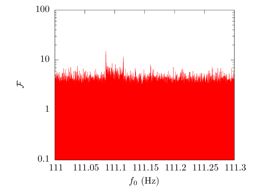
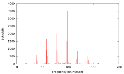
The $\mathcal{J}$-statistic, like the $\mathcal{F}$-statistic, leaks a small amount of residual power into nonorbital sidebands bracketing the central spectral line. Figure 9 displays a close-up of the $\mathcal{J}$-statistic for a strong injection, with $h_{0}=8\times 10^{-25}$. Individual frequency bins are discernible across a $1.1574\times 10^{-4}\,\mathrm{Hz}$ band. The sharp peak coincident with the injected signal splits into sidebands spaced by approximately 20 (out of 200) frequency bins, i.e. $1.157\times 10^{-5}\,\mathrm{Hz}=1/(86400\,\mathrm{s})$. The sidebands are associated with the component of the Earth’s diurnal motion that is not completely removed in the $\mathcal{F}$-statistic, due to approximations like the one leading to (23) and (24). Each diurnal sideband spreads across several adjacent bins; its profile is a $\operatorname*{sinc}$ function produced by the observing window $T_{\mathrm{obs}}$. The signature in Figure 9 is also observed in the $\mathcal{F}$-statistic for an isolated source.

Figure 9: Zoomed-in portion of the $\mathcal{J}$-statistic for an injection with $h_{0}=8\times 10^{-25}$, showing diurnal sidebands (six clearly discernible). Each frequency bin covers $\Delta f_{\mathrm{drift}}=5.787\times 10^{-7}\,\mathrm{Hz}$. Frequency bin number 100 corresponds to the injection frequency $f_{\star}=111.1\,\mathrm{Hz}$. The sidebands are $\approx 20$ frequency bins apart, i.e., $1/(86400\,\mathrm{s})$.

Appendix B Cramér-Rao lower bound for the $\mathcal{J}$-statistic

In general, the Cramér-Rao lower bound (CRLB) of a model parameter $\theta$ estimated from noisy measurements is the minimum possible variance of any unbiased estimator of $\theta$. The CRLB depends on the PDF of the observed data, specifically its curvature in the neighbourhood of the true value of $\theta$. The more sensitively the PDF depends on the parameter (the greater the curvature, in other words), the more accurately the parameter can be estimated.

Let $x(t)=h(t;\bm{\theta})+n(t)$ represent the output from a single interferometer in a gravitational-wave observatory, where $h(t;\bm{\theta})$ is the signal defined by (12)–(16), $n(t)$ represents stationary Gaussian noise, and $\bm{\theta}=(f_{0},a_{0},\phi_{a}=\Omega t_{a})$ is a vector containing the three unknown signal parameters in the search. Let $p(\mathbf{x};\bm{\theta})$ be the PDF of the observed data; here, $\mathbf{x}$ is a vector containing every sample $x(0)$, $x(t_{1})$, $x(t_{2})$, …, $x(T_{\mathrm{obs}})$ of the interferometer output over the full observation $0\leq t_{i}\leq T_{\mathrm{obs}}$. We define the Fisher information matrix $\mathbf{I}$ by its entries

$$I_{ij}=-\left\langle\frac{\partial^{2}\ln p}{\partial\theta_{i}\partial\theta_{j}}\right\rangle,$$ (62)

where $\langle\cdots\rangle$ denotes the expectation value taken over many realisations of the noise. Then the CRLB for the parameter $\theta_{i}$ is (Kay, 1993)

$$\mathrm{var}(\theta_{i})\geq(\mathbf{I}^{-1})_{ii},$$ (63)

where $\mathbf{I}^{-1}$ is the matrix inverse of $\mathbf{I}$, and $(\mathbf{I}^{-1})_{ii}$ symbolises the $i$-th diagonal entry of $\mathbf{I}^{-1}$ as opposed to its trace, i.e. the Einstein summation convention does not apply in (63).

For stationary, Gaussian noise with normalised unit variance, the log likelihood is given by (see Section III)

$$\ln p=-\frac{1}{2}(x-h||x-h)$$ (64)

up to a constant. The model $h(t;\bm{\theta})$ depends on $\bm{\theta}$, and the inner product (19) in (64) is symmetric, so the derivatives of the log likelihood reduce to

$$\frac{\partial\ln p}{\partial\theta_{i}}=\left(x\;\middle|\middle|\;\frac{\partial h}{\partial\theta_{i}}\right)-\left(h\;\middle|\middle|\;\frac{\partial h}{\partial\theta_{i}}\right)$$ (65)

and

$$\frac{\partial^{2}\ln p}{\partial\theta_{i}\partial\theta_{j}}=-\left(\frac{\partial h}{\partial\theta_{i}}\;\middle|\middle|\;\frac{\partial h}{\partial\theta_{j}}\right)+\left(x-h\;\middle|\middle|\;\frac{\partial^{2}h}{\partial\theta_{i}\partial\theta_{j}}\right).$$ (66)

When the ensemble average is taken, the second term in (66) vanishes, because one has $\langle x-h\rangle=0$ for an unbiased estimator. Equations (62) and (66) then imply

$$I_{ij}=\left(\frac{\partial h}{\partial\theta_{i}}\;\middle|\middle|\;\frac{\partial h}{\partial\theta_{j}}\right).$$ (67)

The derivatives $\partial h/\partial\theta_{i}$ are straightforward to evaluate in terms of the signal defined by (12)–(16). Defining $\Phi_{\pm}(t)=\Phi(t)\pm(\Omega t-\phi_{a})$, we obtain

$$\frac{\partial h}{\partial\theta_{i}}=\sum^{4}_{j=1}A_{1j}\frac{\partial h_{1j}}{\partial\theta_{i}}$$ (68)

with

$$\frac{\partial h_{11}}{\partial f_{0}} =-2\pi ta(t)\sin\Phi(t)$$

$$\phantom{=\,}-\pi a_{0}a(t)[\cos\Phi_{+}(t)-\cos\Phi_{-}(t)],$$ (69)

$$\frac{\partial h_{13}}{\partial f_{0}} =2\pi ta(t)\cos\Phi(t)$$

$$\phantom{=\,}-\pi a_{0}a(t)[\sin\Phi_{+}(t)-\sin\Phi_{-}(t)],$$ (70)

$$\frac{\partial h_{11}}{\partial a_{0}} =-\pi f_{0}a(t)[\cos\Phi_{+}(t)-\cos\Phi_{-}(t)],$$ (71)

$$\frac{\partial h_{13}}{\partial a_{0}} =-\pi f_{0}a(t)[\sin\Phi_{+}(t)-\sin\Phi_{-}(t)],$$ (72)

$$\frac{\partial h_{11}}{\partial\phi_{a}} =-\pi f_{0}a_{0}a(t)[\sin\Phi_{+}(t)+\sin\Phi_{-}(t)],$$ (73)

$$\frac{\partial h_{13}}{\partial\phi_{a}} =\pi f_{0}a_{0}a(t)[\cos\Phi_{+}(t)+\cos\Phi_{-}(t)].$$ (74)

In the same way $\partial h_{12}/\partial f_{0}$, $\partial h_{14}/\partial f_{0}$, $\partial h_{12}/\partial a_{0}$, $\partial h_{14}/\partial a_{0}$, $\partial h_{12}/\partial\phi_{a}$, and $\partial h_{14}/\partial\phi_{a}$ are obtained by replacing $a(t)$ with $b(t)$ in (69)–(74) respectively.

When evaluating $I_{ij}$ from (67) using (68)–(74), we note three points. (i) In $\partial h_{1j}/\partial f_{0}$, the first terms on the right-hand sides of (69) and (70) are larger than the second and third terms by a factor of $\approx 2t/a_{0}\gg 1$, implying $\partial h_{11}/\partial f_{0}\approx-2\pi ta(t)\sin\Phi(t)$ and $\partial h_{13}/\partial f_{0}\approx 2\pi ta(t)\cos\Phi(t)$. For example, we have $a_{0}=1.44\,\mathrm{s}$ and $t\leq T_{\mathrm{drift}}=10\,\mathrm{d}$ for Sco X-1. (ii) The beam-pattern functions $a(t)$ and $b(t)$ oscillate about nonzero means. Specifically they are linear combinations of DC terms and sinusoids with periods of $0.5\,\mathrm{d}$ and $1.0\,\mathrm{d}$; see equations (12) and (13) in Ref. (Jaranowski et al., 1998). As the latter periods are typically much shorter than $T_{\mathrm{drift}}$, the relevant timespan for calculating the $\mathcal{J}$-statistic, we can write $(ta||ta)=\frac{1}{3}T_{\mathrm{drift}}^{2}A$, $(tb||tb)=\frac{1}{3}T_{\mathrm{drift}}^{2}B$ and $(ta||tb)=\frac{1}{3}T_{\mathrm{drift}}^{2}C$ plus correction terms of order $(T_{\mathrm{drift}}/1\,\mathrm{d})^{-1}$, with $A$, $B$, and $C$ defined following equation (19). (iii) The off-diagonal products $(\partial h/\partial\theta_{i})(\partial h/\partial\theta_{j})$ with $i\neq j$ are composed of linear combinations of terms oscillating harmonically in time with zero means. Again the oscillation periods are typically much shorter than $T_{\mathrm{drift}}$, yielding $I_{ij}=0$ for $i\neq j$ to a good approximation [plus correction terms of order $\mathrm{max}(P,1\,\mathrm{d})/T_{\mathrm{drift}}\ll 1$]. For example, $(\partial h/\partial f_{0})(\partial h/\partial a_{0})$ is a linear combination of terms proportional to $\sin(\Omega t-\phi_{a})\cos^{2}\Phi(t)$, $\sin(\Omega t-\phi_{a})\cos\Phi(t)\sin\Phi(t)$ and $\sin(\Omega t-\phi_{a})\sin^{2}\Phi(t)$, which oscillate proportional to $\exp[\pm 2i\Phi(t)\pm i\Omega t]$ and $\exp(\pm i\Omega t)$ when expanded. Likewise, $(\partial h/\partial a_{0})(\partial h/\partial\phi_{a})$ is a linear combination of terms proportional to $\sin 2(\Omega t-\phi_{a})$ multiplied by $\cos^{2}\Phi(t)$, $\cos\Phi(t)\sin\Phi(t)$, and $\sin^{2}\Phi(t)$, which oscillate proportional to $\exp[\pm 2i\Phi(t)\pm 2i\Omega t]$ and $\exp(\pm 2i\Omega t)$ when expanded.

Putting together points (i)–(iii) above, we find that the Fisher information matrix is approximately diagonal, i.e. $I_{ij}\approx\mathrm{diag}(I_{f_{0}f_{0}},I_{a_{0}a_{0}},I_{\phi_{a}\phi_{a}})$, with

$$I_{f_{0}f_{0}} =\frac{2T_{\mathrm{obs}}^{2}I_{a_{0}a_{0}}}{3f_{0}^{2}},$$ (75)

$$I_{a_{0}a_{0}} =\pi^{2}f_{0}^{2}[A(A_{11}^{2}+A_{13}^{2})+B(A_{12}^{2}+A_{14}^{2})$$

$$\phantom{=}+2C(A_{11}A_{12}+A_{13}A_{14})],$$ (76)

$$I_{\phi_{a}\phi_{a}} =a_{0}^{2}I_{a_{0}a_{0}}.$$ (77)

The factor $[\cdots]$ in square brackets in (76) equals twice the noncentrality parameter $\lambda$ appearing in the chi-squared PDF of the $\mathcal{F}$-statistic, i.e., $p(2\mathcal{F})=\chi^{2}(2\mathcal{F};4,\lambda)$; see Section III A in Ref. (Suvorova et al., 2016). The CRLBs on the three parameters follow directly from (63):

$$\mathrm{var}(f_{0}) \geq\frac{3f_{0}^{2}}{2T_{\mathrm{obs}}^{2}I_{a_{0}a_{0}}},$$ (78)

$$\mathrm{var}(a_{0}) \geq\frac{1}{I_{a_{0}a_{0}}},$$ (79)

$$\mathrm{var}(\phi_{a}) \geq\frac{1}{a^{2}_{0}I_{a_{0}a_{0}}}.$$ (80)

Appendix C False alarm and dismissal rates

Figure 10: Correlations and maximisation in the HMM log likelihood statistics for the illustrative, three-step example in Appendix C: PDF of the sum of three $\mathcal{F}$- or $\mathcal{J}$-statistic values (red histogram); maximum log likelihood of nine arbitrary, independent Viterbi paths (blue curve); maximum log likelihood of the nine Viterbi paths in a single realisation of synthetic noise (green curve).

Figure 11: Least-squares fit of a Gumbel law (84) (red curve) to $K(z,\lambda=0)$ in (81) derived from Monte-Carlo simulations (blue curve) for the representative example $N_{T}=37$ and $N_{Q}=1.73\times 10^{6}$. The best fit is for $a=10.0$ and $b=268$.

Table 7: Gumbel law [see (84)] parameters $a(N_{T},N_{Q})$ and $b(N_{T},N_{Q})$ for empirical fits to $K(z,\lambda=0)$ as functions of $N_{T}$ and $N_{Q}$ in ranges useful in practice. The RMSE column gives the root-mean-square error between the fit and empirical cumulative distribution function from Monte-Carlo simulations; one finds RMSE $<1\%$. The values of $N_{Q}$ are equally spaced logarithmically.

	$N_{Q}=1.73\times 10^{6}$			$N_{Q}=1.73\times 10^{6}/\sqrt{10}$			$N_{Q}=1.73\times 10^{6}/10$
$N_{T}$	$a$	$b$	RMSE	$a$	$b$	RMSE	$a$	$b$	RMSE
1	$2.13$	$32.13$	$7.8\times 10^{-3}$	$2.13$	$32.13$	$7.8\times 10^{-3}$	$2.13$	$32.13$	$7.8\times 10^{-3}$
5	$2.67$	$73.83$	$6.5\times 10^{-3}$	$2.67$	$73.83$	$6.5\times 10^{-3}$	$2.67$	$73.83$	$6.5\times 10^{-3}$
10	$3.35$	$119.27$	$6.0\times 10^{-3}$	$3.35$	$119.27$	$6.0\times 10^{-3}$	$3.35$	$119.27$	$6.0\times 10^{-3}$
15	$3.46$	$162.99$	$5.7\times 10^{-3}$	$3.46$	$162.99$	$5.7\times 10^{-3}$	$3.46$	$162.99$	$5.7\times 10^{-3}$
20	$3.44$	$205.59$	$5.5\times 10^{-3}$	$3.44$	$205.59$	$5.5\times 10^{-3}$	$3.44$	$205.59$	$5.5\times 10^{-3}$
25	$3.75$	$247.62$	$5.3\times 10^{-3}$	$3.75$	$247.62$	$5.3\times 10^{-3}$	$3.75$	$247.62$	$5.3\times 10^{-3}$
30	$4.25$	$289.34$	$5.1\times 10^{-3}$	$4.25$	$289.34$	$5.1\times 10^{-3}$	$4.25$	$289.34$	$5.1\times 10^{-3}$
37	$4.55$	$347.18$	$4.6\times 10^{-3}$	$4.55$	$347.18$	$4.6\times 10^{-3}$	$4.55$	$347.18$	$4.6\times 10^{-3}$

In order to calculate the false alarm probability $P_{\mathrm{a}}$ and false dismissal probability $P_{\mathrm{d}}$ for the algorithm developed in this paper, one needs the PDFs of the Viterbi probabilities after $k$ steps of the HMM in the absence and presence of a signal respectively. As far as the authors know, no general formula for these HMM PDFs exists in the literature for a chi-squared–distributed estimator like the $\mathcal{F}$-statistic or $\mathcal{J}$-statistic. In this appendix, we review why the HMM maximisation step makes it hard to calculate the score PDF (section C.1), present an approximate, empirical distribution whose form is suggested by extreme value theory (section C.2), and quantify $P_{\mathrm{a}}$ and $P_{\mathrm{d}}$ in terms of the empirical distribution (section C.3). We improve on a first attempt at these calculations in Ref. (Suvorova et al., 2016) and compute the probability of outliers more realistically.

C.1 Viterbi path correlation and maximisation

Equation (33) in Ref. (Suvorova et al., 2016) estimates $P_{\mathrm{a}}$ crudely by assuming that $\max\log\Pr(Q|O)$ follows a central chi-squared distribution with $4k$ degrees of freedom after $k$ HMM steps, because $2\mathcal{F}=\log L_{o(t_{k})q(t_{k})}$ is drawn from the PDF $p(2\mathcal{F})=\chi^{2}(2\mathcal{F};4,0)$ in the absence of a signal, and the chi-squared distribution is additive. However, this assumption breaks down on two counts. First, the nonlinear maximisation operator in the Viterbi algorithm returns values from the tail of $\chi^{2}(2\mathcal{F};4,0)$, because $\chi^{2}(2\mathcal{F};4,0)$ is sampled $N_{Q}$ times, once for each possible transition from the previous step. Second, the Viterbi paths overlap partially, so the random numbers $\log L_{o(t_{j})q(t_{j})}$ for $1\leq j\leq k$ are not independent and identically distributed. Exactly the same issues arise, if the frequency domain estimator at each HMM step is the $\mathcal{J}$-statistic instead of the $\mathcal{F}$-statistic.

Consider all admissible paths following the transition rule in equation (3), that end in state $q_{i}$ after the $k$-th HMM step. Label the log likelihood of each path by $x_{p}=\log\Pr(Q|O)$, with $1\leq p\leq 3^{k}$. We wish to compute the cumulative probability that $\max_{p}x_{p}$ is less than $z$, viz.

$$K(z;\lambda)=\Pr(x_{1}<z,\cdots,x_{3^{k}}<z)$$ (81)

where $\lambda$ is the non-centrality parameter (zero for the case of noise, and positive for signal plus noise) which is related to the gravitational wave signal strength by equation (28) in Section III.3.

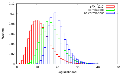
A difficulty arises because $x_{1},...,x_{3^{k}}$ are correlated, so the joint distribution cannot be written as a product of individual probabilities. We illustrate with an example. Consider all admissible paths up to $k=3$ ending in $q_{3}$. We have $x_{1}=X(1,1)+X(2,2)+X(3,3)$ for the path $\{q_{1},q_{2},q_{3}\}$, $x_{2}=X(2,1)+X(2,2)+X(3,3)$ for the path $\{q_{2},q_{2},q_{3}\}$, and so on, where $X(i,j)$ are independent samples of the $\mathcal{F}$-statistic or $\mathcal{J}$-statistic in state $q_{i}$ at the $j$-th HMM step. We can write the sums in matrix notation as $\mathbf{x}=A\mathbf{u}$ with $\mathbf{x}=(x_{1},\cdots,x_{9})^{T}$, $\mathbf{u}=[X(1,1),\allowbreak X(2,1),\allowbreak X(3,1),\allowbreak X(4,1),\allowbreak X(5,1),\allowbreak X(2,2),\allowbreak X(3,2),\allowbreak X(4,2),\allowbreak X(3,3)]^{T}$ and

$$A=\left(\begin{matrix}1&0&0&0&0&1&0&0&1\\ 0&1&0&0&0&1&0&0&1\\ 0&0&1&0&0&1&0&0&1\\ 0&1&0&0&0&0&1&0&1\\ 0&0&1&0&0&0&1&0&1\\ 0&0&0&1&0&0&1&0&1\\ 0&0&1&0&0&0&0&1&1\\ 0&0&0&1&0&0&0&1&1\\ 0&0&0&0&1&0&0&1&1\end{matrix}\right).$$ (82)

The covariance of $\mathbf{x}$ is

$$\langle x_{i},x_{j}\rangle=AA^{T}=\left(\begin{matrix}3&2&2&1&1&1&1&1&1\\ 2&3&2&2&1&1&1&1&1\\ 2&2&3&1&2&1&2&1&1\\ 1&2&1&3&2&2&1&1&1\\ 1&1&2&2&3&2&2&1&1\\ 1&1&1&2&2&3&1&2&1\\ 1&1&2&1&2&1&3&2&2\\ 1&1&1&1&1&2&2&3&2\\ 1&1&1&1&1&1&2&2&3\\ \end{matrix}\right).$$ (83)

Equation (83) is clearly not diagonal. At the time of writing, it is unclear how to fold equation (83) analytically into the computation of $K(z,\lambda=0)$.

C.2 Log likelihood PDF

Although it is challenging to calculate the PDF of $\max_{p}x_{p}=\max_{Q}\log\Pr(Q|O)$ theoretically, it is relatively simple, albeit time-consuming, to compute it empirically. Figure 10 plots three histograms for the illustrative example of a three-step HMM: the PDF of the sum of three independent $\mathcal{F}$- or $\mathcal{J}$-statistic values, which matches a central chi-squared distribution with 12 degrees of freedom (red histogram); the PDF of $\delta_{q_{i}}(t_{N_{T}})$ without taking correlations into account, i.e. the maximum log likelihood for any nine independent paths, each path comprising three independent $\mathcal{F}$- or $\mathcal{J}$-statistic samples (blue histogram); and the PDF of $\delta_{q_{i}}(t_{N_{T}})$ taking correlations into account, i.e. the maximum log likelihood from the nine paths in the vector $\mathbf{x}$ for a single realisation of a synthetic observation (green histogram). The PDF taking correlations into account peaks to the right of the PDF that neglects correlations, because extreme $\mathcal{F}$-statistic values are likely to end up in multiple paths (if they are large) or end up in few paths (if they are small). Correlations therefore play a significant role.

Extreme value theory states that there exist three PDF families that describe asymptotically the maximum of $N^{\prime}$ samples of a random variable for $N^{\prime}\gg 1$: the Weibull, Gumbel and Fréchet laws (Sornette, 2004). The families correspond to light, exponential, and heavy tails respectively in the PDF of the underlying random variable. Here we seek empirically the best fit to $K(z,\lambda)$ in (81). The underlying variable $x_{p}$ is crudely chi-squared distributed, even when the correlations discussed in Section C.1 are included; the tail is exponential, which is easy to verify by replotting Figure 10 on log-linear axes. Testing by trial and error confirms that the Gumbel Law is a superior fit compared to the Weibull and Fréchet laws, with

$$K(z,\lambda=0)=\exp\{-\exp[-(z-b)/a]\},$$ (84)

where $a(N_{T},N_{Q})$ and $b(N_{T},N_{Q})$ are dimensionless parameters. Note that 84 strictly applies to a variable that takes values along the whole real line. In this application, in contrast, we have $z\geq 0$. But we also have $b\gg a$ and hence $K(0)\approx 0$ to a good approximation.

An example of the fit for $N_{T}=37$ and $M=1.73\times 10^{6}$ is graphed in Figure 11. The plot confirms visually, that the fit is good, with root-mean-square error $\approx 1.46\times 10^{-2}$. In a Sco X-1 search, these values of $N_{T}$ and $N_{Q}$ correspond to an observation with $T_{\mathrm{drift}}=10\,\mathrm{d}$ and $T_{\mathrm{obs}}=370\,\mathrm{d}$, covering a bandwidth of $N_{Q}\Delta f_{\mathrm{drift}}=1.0\,\mathrm{Hz}$.

Table 7 presents $a$, $b$ and the root-mean-square error of the fit for various practically motivated choices of $N_{T}$ and $N_{Q}$. The error is generally less than one per cent, giving confidence that (84) is a good approximation.

When a signal is introduced (i.e. $\lambda>0$), the situation is complicated considerably, because the optimal path may travel through some states containing the signal (drawn from a non-central chi-squared distribution) and others containing noise only (drawn from a central chi-squared distribution). We simplify things by considering the extreme case, where the optimal path exactly matches the signal path. The simplification is conservative, because in a real search it is possible for the optimal path to include some noise-only bins yet still exceed the threshold for a detection.

In the extreme case, the cumulative distribution function for $\lambda>0$ is given by

$$K(z;\lambda)=1-Q_{k/2}(\sqrt{\lambda},\sqrt{z})$$ (85)

after $k$ HMM steps, where $Q_{k/2}$ is the Marcum-Q function,

$$Q_{k/2}(u,v) =\frac{1}{u^{(k/2)-1}}\int_{v}^{\infty}\,\mathrm{d}x\,x^{k/2}$$ (86)

$$\phantom{=}\exp[-(x^{2}+u^{2})/2]I_{(k/2)-1}(ux),$$

and $I_{(k/2)-1}$ is a modified Bessel function of order $(k/2)-1$.

C.3 Receiver operator characteristic (ROC) curve

The HMM tracker determines the log likelihood $z$ that a given set of parameters corresponds to a signal. We choose a threshold log likelihood $z_{\mathrm{th}}$ and claim a detection for $z>z_{\mathrm{th}}$. The false alarm probability, $P_{\mathrm{a}}$, quantifies how often pure noise gives $z>z_{\mathrm{th}}$, causing a spurious detection. Given $P_{\mathrm{a}}$, we solve

$$K(z_{\mathrm{th}};\lambda=0)=1-P_{\mathrm{a}}$$ (87)

for $z_{\mathrm{th}}$.

Once $P_{\mathrm{a}}$ and hence $z_{\mathrm{th}}$ are fixed, some signals by chance fail to be detected because they are too weak, relative to the noise, to produce $z>z_{\mathrm{th}}$. The false dismissal probability, $P_{\mathrm{d}}$, quantifies the probability of this outcome. Upon choosing $P_{\mathrm{d}}$, we determine the weakest signal that can be reliably detected by solving

$$K(z_{\mathrm{th}};\lambda)=P_{\mathrm{d}}$$ (88)

for $\lambda$ and hence $h_{0}$ via (28).

Figure 12(a) displays ROC curves for four values of $\lambda$. Each curve shows the tradeoff of $P_{\mathrm{a}}$ (on the horizontal axis) against detection rate $1-P_{\mathrm{d}}$ (on the vertical axis). The results are replotted on logarithmic axes in Figure 12(b) to magnify the edges of the plot. The detection probability increases, as $\lambda$ increases. It also rises superlinearly (linearly) with $P_{\mathrm{a}}$ for $P_{\mathrm{a}}\lesssim 0.1$ ($P_{\mathrm{a}}\gtrsim 0.1$).

Figure 13 shows how the detection probability increases as more data blocks are processed, again for the same four values of $\lambda$ as Figure 12. As expected, the detection probability rises, as $N_{T}$ and hence $T_{\mathrm{obs}}$ increase, keeping $T_{\mathrm{drift}}$ fixed.

(a)

(b)

Figure 12: Receiver operator characteristic curves for $N_{T}=37$ blocks and four representative choices of $\lambda$, ranging from a strong signal ($\lambda=10$, red curve) to a signal too weak to be reliably detected at the commonly used false alarm probability $P_{\mathrm{a}}=0.1$ ($\lambda=3.5$, purple curve). At each point along a curve, the vertical axis indicates the detection probability $1-P_{\mathrm{d}}$, and the horizontal axis indicates the false alarm probability $P_{\mathrm{a}}$. (a) Linear scale. (b) Log-log scale. Detection occurs when the optimal path exactly matches $f_{\star}(t)$, c.f. Viterbi score in Section IV.3.

Figure 13: Detection probability versus number of HMM steps $N_{T}$ with $T_{\mathrm{drift}}=10\,\mathrm{d}$ for the same four values of $\lambda$ as in Figure 12. Detection occurs when the optimal path exactly matches $f_{\star}(t)$, c.f. Viterbi score in Section IV.3.

References

- Riles (2013) K. Riles, Progress in Particle and Nuclear Physics 68, 1 (2013).
- Wagoner (1984) R. V. Wagoner, Astrophys. J. 278, 345 (1984).
- Bildsten (1998) L. Bildsten, The Astrophysical Journal Letters 501, L89 (1998), astro-ph/9804325 .
- Ushomirsky et al. (2000) G. Ushomirsky, C. Cutler, and L. Bildsten, MNRAS 319, 902 (2000).
- Melatos and Payne (2005) A. Melatos and D. J. B. Payne, Astrophys. J. 623, 1044 (2005).
- Vigelius and Melatos (2009) M. Vigelius and A. Melatos, Monthly Notices of the Royal Astronomical Society 395, 1972 (2009), arXiv:0902.4264 [astro-ph.HE] .
- Priymak et al. (2011) M. Priymak, A. Melatos, and D. J. B. Payne, Monthly Notices of the Royal Astronomical Society 417, 2696 (2011), arXiv:1109.1040 [astro-ph.HE] .
- Owen et al. (1998) B. Owen, L. Lindblom, C. Cutler, B. Schutz, A. Vecchio, and N. Andersson, Physical Review D 58, 084020 (1998).
- Bondarescu et al. (2007) R. Bondarescu, S. A. Teukolsky, and I. Wasserman, Phys. Rev. D 76, 064019 (2007), arXiv:0704.0799 .
- Bondarescu and Wasserman (2013) R. Bondarescu and I. Wasserman, Astrophys. J. 778, 9 (2013), arXiv:1305.2335 [astro-ph.SR] .
- Haskell et al. (2015) B. Haskell, M. Priymak, A. Patruno, M. Oppenoorth, A. Melatos, and P. D. Lasky, Monthly Notices of the Royal Astronomical Society 450, 2393 (2015), arXiv:1501.06039 [astro-ph.SR] .
- Aasi et al. (2014a) J. Aasi, B. P. Abbott, R. Abbott, T. Abbott, M. R. Abernathy, T. Accadia, F. Acernese, K. Ackley, C. Adams, T. Adams, and et al., Phys. Rev. D 90, 062010 (2014a), arXiv:1405.7904 [gr-qc] .
- Goetz and Riles (2011) E. Goetz and K. Riles, Classical and Quantum Gravity 28, 215006 (2011), arXiv:1103.1301 [gr-qc] .
- Meadors et al. (2016) G. D. Meadors, E. Goetz, and K. Riles, Classical and Quantum Gravity 33, 105017 (2016), arXiv:1512.02105 [gr-qc] .
- Aasi et al. (2015a) J. Aasi, B. P. Abbott, R. Abbott, T. Abbott, M. R. Abernathy, F. Acernese, K. Ackley, C. Adams, T. Adams, P. Addesso, and et al., Astrophys. J. 813, 39 (2015a), arXiv:1412.5942 [astro-ph.HE] .
- Sammut et al. (2014) L. Sammut, C. Messenger, A. Melatos, and B. Owen, Physical Review D 89, 043001 (2014).
- Messenger and Woan (2007) C. Messenger and G. Woan, Classical and Quantum Gravity 24, S469 (2007).
- Abadie et al. (2011) J. Abadie, B. P. Abbott, R. Abbott, M. Abernathy, T. Accadia, F. Acernese, C. Adams, R. Adhikari, P. Ajith, B. Allen, G. S. Allen, E. Amador Ceron, R. S. Amin, S. B. Anderson, W. G. Anderson, F. Antonucci, and et al. (LIGO Scientific Collaboration and Virgo Collaboration), Phys. Rev. Lett. 107, 271102 (2011).
- Ballmer (2006) S. W. Ballmer, Classical and Quantum Gravity 23, S179 (2006).
- Dhurandhar et al. (2008) S. Dhurandhar, B. Krishnan, H. Mukhopadhyay, and J. T. Whelan, Physical Review D 77, 082001 (2008).
- Chung et al. (2011) C. T. Y. Chung, A. Melatos, B. Krishnan, and J. T. Whelan, MNRAS 414, 2650 (2011).
- Whelan et al. (2015) J. T. Whelan, S. Sundaresan, Y. Zhang, and P. Peiris, Physical Review D 91, 102005 (2015).
- Sun et al. (2016) L. Sun, A. Melatos, P. D. Lasky, C. T. Y. Chung, and N. S. Darman, ArXiv e-prints (2016), arXiv:1610.00059 [gr-qc] .
- van der Putten et al. (2010) S. van der Putten, H. J. Bulten, J. F. J. van den Brand, and M. Holtrop, Journal of Physics: Conference Series 228, 012005 (2010).
- Messenger et al. (2015) C. Messenger, H. Bulten, S. Crowder, V. Dergachev, D. Galloway, E. Goetz, R. Jonker, P. Lasky, G. Meadors, A. Melatos, S. Premachandra, K. Riles, L. Sammut, E. Thrane, J. Whelan, and Y. Zhang, Physical Review D 92, 023006 (2015).
- Leaci and Prix (2015) P. Leaci and R. Prix, Phys. Rev. D 91, 102003 (2015), arXiv:1502.00914 [gr-qc] .
- Bildsten et al. (1997) L. Bildsten, D. Chakrabarty, J. Chiu, M. H. Finger, D. T. Koh, R. W. Nelson, T. A. Prince, B. C. Rubin, D. M. Scott, M. Stollberg, B. A. Vaughan, C. A. Wilson, and R. B. Wilson, The Astrophysical Journal Supplement Series 113, 367 (1997).
- Baykal and Oegelman (1993) A. Baykal and H. Oegelman, Astronomy and Astrophysics (ISSN 0004-6361) 267, 119 (1993).
- de Kool and Anzer (1993) M. de Kool and U. Anzer, Monthly Notices of the Royal Astronomical Society (ISSN 0035-8711) 262, 726 (1993).
- Romanova et al. (2004) M. M. Romanova, G. V. Ustyugova, A. V. Koldoba, and R. V. E. Lovelace, The Astrophysical Journal 616, L151 (2004).
- Taam and Fryxell (1988) R. E. Taam and B. A. Fryxell, The Astrophysical Journal 327, L73 (1988).
- Baykal et al. (1991) A. Baykal, A. Alpar, and U. Kiziloglu, Astronomy and Astrophysics (ISSN 0004-6361) 252, 664 (1991).
- Baykal (1997) A. Baykal, Astronomy and Astrophysics (1997).
- Suvorova et al. (2016) S. Suvorova, L. Sun, A. Melatos, W. Moran, and R. J. Evans, Phys. Rev. D 93, 123009 (2016), arXiv:1606.02412 [astro-ph.IM] .
- Quinn and Hannan (2001) B. G. Quinn and E. J. Hannan, The Estimation and Tracking of Frequency (Cambridge University Press, 2001) p. 266.
- Paris and Jauffret (2003) S. Paris and C. Jauffret, IEEE Transactions on Aerospace and Electronic Systems 39, 439 (2003).
- White and Elliott (2002) L. B. White and R. J. Elliott, IEEE Transactions on Signal Processing 50, 1205 (2002).
- Viterbi (1967) A. Viterbi, IEEE Transactions on Information Theory 13, 260 (1967).
- The LIGO Scientific Collaboration et al. (2017) The LIGO Scientific Collaboration, the Virgo Collaboration, B. P. Abbott, R. Abbott, T. D. Abbott, F. Acernese, K. Ackley, C. Adams, T. Adams, P. Addesso, and et al., ArXiv e-prints (2017), arXiv:1704.03719 [gr-qc] .
- Premachandra et al. (2016) S. S. Premachandra, D. K. Galloway, J. Casares, D. T. Steeghs, and T. R. Marsh, Astrophys. J. 823, 106 (2016), arXiv:1604.03233 [astro-ph.HE] .
- Galloway et al. (2014) D. K. Galloway, S. Premachandra, D. Steeghs, T. Marsh, J. Casares, and R. Cornelisse, The Astrophysical Journal 781, 14 (2014).
- Baum et al. (1970) L. E. Baum, T. Petrie, G. Soules, and N. Weiss, Ann. Math. Statist. 41, 164 (1970).
- Jaranowski et al. (1998) P. Jaranowski, A. Królak, and B. F. Schutz, Physical Review D 58, 063001 (1998).
- Aasi et al. (2015b) J. Aasi, B. P. Abbott, R. Abbott, T. Abbott, M. R. Abernathy, F. Acernese, K. Ackley, C. Adams, T. Adams, T. Adams, and et al., Phys. Rev. D 91, 022004 (2015b), arXiv:1410.8310 [astro-ph.IM] .
- Prix (2011) R. Prix, LIGO Report T0900149 (June 2011).
- Sornette (2004) D. Sornette, Critical phenomena in natural sciences : chaos, fractals, selforganization and disorder : concepts and tools, 2nd ed. by Didier Sornette. Springer series in synergetics. (Springer, 2004).
- Steeghs and Casares (2002) D. Steeghs and J. Casares, Astrophys. J. 568, 273 (2002), astro-ph/0107343 .
- Hobbs et al. (2010) G. Hobbs, A. G. Lyne, and M. Kramer, Monthly Notices of the Royal Astronomical Society 402, 1027 (2010).
- Shannon and Cordes (2010) R. M. Shannon and J. M. Cordes, Astrophys. J. 725, 1607 (2010).
- Cordes and Helfand (1980) J. M. Cordes and D. J. Helfand, Astrophys. J. 239, 640 (1980).
- Price et al. (2012) S. Price, B. Link, S. N. Shore, and D. J. Nice, Monthly Notices of the Royal Astronomical Society 426, 2507 (2012).
- Alpar et al. (1986) M. A. Alpar, R. Nandkumar, and D. Pines, Astrophys. J. 311, 197 (1986).
- Cheng (1987) K. S. Cheng, The Astrophysical Journal 321, 799 (1987).
- Jones (1990) P. Jones, Monthly Notices of the Royal Astronomical Society 246 (1990).
- Lyne et al. (2010) A. Lyne, G. Hobbs, M. Kramer, I. Stairs, and B. Stappers, Science 329, 408 (2010).
- Melatos and Link (2014) A. Melatos and B. Link, Monthly Notices of the Royal Astronomical Society 437, 21 (2014).
- Aasi et al. (2013a) J. Aasi, J. Abadie, B. P. Abbott, R. Abbott, T. D. Abbott, M. Abernathy, T. Accadia, F. Acernese, C. Adams, T. Adams, and et al., Physical Review D 87, 042001 (2013a), arXiv:1207.7176 [gr-qc] .
- Aasi et al. (2016a) J. Aasi, B. P. Abbott, R. Abbott, T. D. Abbott, M. R. Abernathy, F. Acernese, K. Ackley, C. Adams, T. Adams, P. Addesso, and et al., Physical Review D 93, 042007 (2016a), arXiv:1510.03621 [astro-ph.IM] .
- Walsh et al. (2016) S. Walsh, M. Pitkin, M. Oliver, S. D’Antonio, V. Dergachev, A. Królak, P. Astone, M. Bejger, M. Di Giovanni, O. Dorosh, S. Frasca, P. Leaci, S. Mastrogiovanni, A. Miller, C. Palomba, M. A. Papa, O. J. Piccinni, K. Riles, O. Sauter, and A. M. Sintes, Phys. Rev. D 94, 124010 (2016), arXiv:1606.00660 [gr-qc] .
- Aasi et al. (2013b) J. Aasi, J. Abadie, B. P. Abbott, R. Abbott, T. Abbott, M. R. Abernathy, T. Accadia, F. Acernese, C. Adams, T. Adams, and et al., Physical Review D 88, 102002 (2013b), arXiv:1309.6221 [gr-qc] .
- Aasi et al. (2016b) J. Aasi, B. P. Abbott, R. Abbott, T. D. Abbott, M. R. Abernathy, F. Acernese, K. Ackley, C. Adams, T. Adams, P. Addesso, and et al., Physical Review D 93, 042006 (2016b), arXiv:1510.03474 [gr-qc] .
- Abadie et al. (2010) J. Abadie, B. P. Abbott, R. Abbott, M. Abernathy, C. Adams, R. Adhikari, P. Ajith, B. Allen, G. Allen, E. Amador Ceron, and et al., The Astrophysical Journal 722, 1504 (2010), arXiv:1006.2535 [gr-qc] .
- Abbott et al. (2008) B. Abbott, R. Abbott, R. Adhikari, P. Ajith, B. Allen, G. Allen, R. Amin, S. B. Anderson, W. G. Anderson, M. A. Arain, and et al., The Astrophysical Journal Letters 683, L45 (2008), arXiv:0805.4758 .
- Aasi et al. (2014b) J. Aasi, J. Abadie, B. P. Abbott, R. Abbott, T. Abbott, M. R. Abernathy, T. Accadia, F. Acernese, C. Adams, T. Adams, and et al., Astrophys. J. 785, 119 (2014b), arXiv:1309.4027 [astro-ph.HE] .
- Abadie et al. (2011) J. Abadie, B. P. Abbott, R. Abbott, M. Abernathy, T. Accadia, F. Acernese, C. Adams, R. Adhikari, C. Affeldt, B. Allen, and et al., The Astrophysical Journal 737, 93 (2011), arXiv:1104.2712 [astro-ph.HE] .
- Abbott et al. (2010) B. P. Abbott, R. Abbott, F. Acernese, R. Adhikari, P. Ajith, B. Allen, G. Allen, M. Alshourbagy, R. S. Amin, S. B. Anderson, and et al., The Astrophysical Journal 713, 671 (2010), arXiv:0909.3583 [astro-ph.HE] .
- Warszawski and Melatos (2013) L. Warszawski and A. Melatos, Monthly Notices of the Royal Astronomical Society 428, 1911 (2013), arXiv:1210.2203 [astro-ph.HE] .
- Melatos et al. (2015) A. Melatos, J. A. Douglass, and T. P. Simula, Astrophys. J. 807, 132 (2015).
- Ashton et al. (2015) G. Ashton, D. I. Jones, and R. Prix, Phys. Rev. D 91, 062009 (2015), arXiv:1410.8044 [gr-qc] .
- Kay (1993) S. M. Kay, Fundamentals of Statistical Signal Processing: Estimation Theory (Prentice-Hall, Inc., Upper Saddle River, NJ, USA, 1993).