iSIRA: Integrated Shift-Invert Residual Arnoldi Method for Graph Laplacian Matrices from Big Data

Abstract

The eigenvalue problem of a graph Laplacian matrix $L$ arising from a simple, connected and undirected graph has been given more attention due to its extensive applications, such as spectral clustering, community detection, complex network, image processing and so on. The associated graph Laplacian matrix is symmetric, positive semi-definite, and is usually large and sparse. Computing some smallest positive eigenvalues and corresponding eigenvectors is often of interest.

However, the singularity of $L$ makes the classical eigensolvers inefficient since we need to factorize $L$ for the purpose of solving large and sparse linear systems exactly. The next difficulty is that it is usually time consuming or even unavailable to factorize a large and sparse matrix arising from real network problems from big data such as social media transactional databases, and sensor systems because there is in general not only local connections.

In this paper, we propose an eignsolver based on the inexact residual Arnoldi [18, 19] method together with an implicit remedy of the singularity and an effective deflation for convergent eigenvalues. Numerical experiments reveal that the integrated eigensolver outperforms the classical Arnoldi/Lanczos method for computing some smallest positive eigeninformation provided the LU factorization is not available.

Mathematics Subject Classification (2010):

15B99 65F50 65N25

1 Introduction

Graph-based approaches have been an increasingly favorable tool for representation, processing and explosion of interests in studying large networks because of the potential for capturing dependence structure of the data set. One of the research problems of interests is to compute some eigenpairs based on the so-called Graph Laplacians Eigenvalue Problem (GLEP). The GLEPs appear in many areas, such as combinatorial optimization, clustering, embedding, dimensionality reduction, data representation, community detection, image processiong and complex networks [22, 31, 26, 3, 39, 38, 24, 37, 30, 1, 7, 11, 5, 4, 27]. For more applications on this topic, we refer to as [21].

1.1 The Graph Laplacian Matrix

Given a simple (no multiple edges or loops), connected and undirected graph $\mathcal{G}=\left(\mathcal{V},\mathcal{E}\right)$, where $\mathcal{V}$ is the vertex set with $|\mathcal{V}|=n$ and $\mathcal{E}$ is the edge set that describes the connection between vertices. In addition, the degree of each vertex $v\in\mathcal{V}$ is the number of edges which incident to $v$. According to the information, the adjacency matrix $A$ as well as the degree matrix $D$ of $\mathcal{G}$ are, respectively, defined by

$$A_{ij}=\left\{\begin{array}[]{cc}1,&\text{if }ij\in\mathcal{E},\\ 0,&\text{if }ij\notin\mathcal{E},\end{array}\right.\quad\text{and}\quad D_{ij}=\left\{\begin{array}[]{cc}\sum_{j=1}^{n}A_{ij},&\text{if }i=j,\\ 0,&\text{if }i\neq j,\end{array}\right.$$

where $1\leq i,j\leq n$. Then the so-called graph Laplacian matrix of $\mathcal{G}$ is defined by $L=D-A$. That is,

$$L_{ij}=\left\{\begin{array}[]{cl}D_{ii},&\text{if }i=j,\\ -1,&\text{if }i\text{ and }j\text{ are adjacent,}\\ 0,&\text{otherwise,}\end{array}\right.\ 1\leq i,j\leq n.$$ (1.1)

Below, we recall some properties of the graph Laplacian matrix.

Definition 1.1.

Recall the definitions of the irreducible matrix and the M-matrix.

• A matrix is called an irreducible matrix if it is not similar to a block upper triangular matrix using a permutation matrix.

• A square matrix is said to be an M-matrix if its off-diagonal entries are less than or equal to zero with eigenvalues whose real parts are positive.

Theorem 1.2 ([23]).

Let $L$ be a graph Laplacain matrix induced from a simple, connected and undirected graph. Then

• $L$ is a singular irreducible M-matrix.

• $L$ has exactly one zero eigenvalue and the corresponding eigenvector is the all-one vector.

Remark 1.3.

If we additionally associate $\mathcal{G}$ with a symmetric nonnegative weight matrix $W\in\mathbb{R}^{n\times n}$ with zero diagonal entries. That is, the entry $W_{ij}$ denotes the nonnegative edge weight between vertices $i,j$ if $ij\in\mathcal{E}$ and $W_{ij}=0$ in the case either $i=j$ or vertex $i$ as well as $j$ are not connected. At this time, the diagonal degree matrix $D_{w}$ is composed of the total weight on edges connected to each vertex and $L_{w}:=D_{w}-W$ is called the weighted Laplacian $L_{w}$ associated to $W$. It is of course that weights on edges can be signed. This study, we only focus on positive weights. To simplify the notation, we only consider $W=A$, that is the case of the classical Laplacian. Note that the following discussion is also true for a graph Laplacian matrix with positive edge weights.

Finding some smallest positive eigenvalues and the associated eigenvectors of the graph Laplacian matrix (1.1) is a fundamental problem in these applications. Certainly, there have been many excellent theoretical investigations and numerical algorithms for these subjects and these methods, such as the inverse power method [12] and the Anoldi method as well as the Lanczos method [9], Nevertheless, these methods have to continuously solve linear systems of the rank deficient Laplacian matrix generated from a simple, connected and undirected graph. A traditional way to address the singularity problem is to add a small diagonal perturbation matrix. The same trick will be applied to improve the condition number of the problem, through the Tikhonov regularization [35] or the ridge regression [25] in the area of statistics and machine learning. Even the resulting matrix is invertible, for large graph such as the social network, however, there is not only local connections between the vertices and this implies that it is almost impossible to find matrix factorizations for exact solving linear systems involved in an eigensolver. That is, only the most scalable algorithms are practical for a large graph Laplacian matrix.

In this paper we first remedy the problem of singularity of the graph Laplacian matrix. Then, we introduce a technique of eigenvalue deflations as shown in [28, 34, 9, 11] so that we can find the desired eigenvalues in order and exclude the influence of the convergent ones. Finally, we integrate these approaches into the eigensolver called shift-invert residual Arnoldi (SIRA) method [18, 19]. SIRA is an inner-outer iterative eigensolver and the inner linear system is allowed to be solved with the low accuracy. As a result, we propose an inexact inner-outer eigensolver with the cure of sigularity and the aid of deflation.

1.2 Notations and Overview

Throughout this paper, capital Roman and Greek letters indicate matrices and lowercase bold face letters denote vectors. Lowercase Greek letters are the scalars. $I_{n}$ denotes the $n\times n$ identity matrix with the given size $n$, $\mathbf{e}_{j}$ is the $j$th column of the identity matrix $I_{n}$. The notation $\mathbf{1}_{n}$ denotes a all-one $n$-vector. $\mathbf{0}$ represents a zero vector and matrix whose dimension should become evident from the context. We adopt the following MATLAB notations: $\mathbf{v}(i\text{:}j)$ denotes the subvector of the vector $\mathbf{v}$ that consists of the $i$th to the $j$th entries of $\mathbf{v}$. Given a matrix $A$, the slice $A(i\text{:}j,:)$ selects the rows $i$ to $j$ and $A(i,:)$ indicates the $i$th row of $A$. The notation $\cdot^{\top}$ denotes the transpose of vectors or matrices. Other notations will be clearly defined whenever they are used.

The rest of this paper is organized as follows. In Section 2, we revisit the background on the eigenvalue problem of a graph Laplacian matrix $L$ in (1.1). Next, we propose trimming as well as deflating approaches, and review the shift-inverted residual Arnoldi method. In Section 3, we integrate the above techniques and present an iterative eigensolver for solving the large and spare graph Laplacain eigenvalue problems. Numerical experiments and comparisons are presented in Section 4. Finally, we end up by discussing some concluding remarks and further works in Section 5.

2 The Graph Laplacian Eigenvalue Problem

For the graph Laplacian matrix $L$ (1.1) generated from a simple-connected graph with nodes $n$, we study the eigenvalue problem

$$L\mathbf{x}=\lambda\mathbf{x},$$ (2.1)

where $L$ is symmetric positive semi-definite with the unique kernel vector $\mathbf{1}_{n}$ as proposed in Theorem 1.2. We are interested in finding some smallest positive eigenvalues and the associated eigenvectors of (2.1).

It is well know that the shift-invert spectral transformation [28, 2, 34, 9] is used to enhance convergence to a desired portion of the spectrum. Specifically, to find eigenvalues of $L\mathbf{x}=\lambda\mathbf{x}$ near a target $\sigma$, which is not an eigenvalue of $L$, the shift-invert spectral transformation is to consider the corresponding shift-and-invert eigenvalue problem $(L-\sigma I_{n})^{-1}\mathbf{x}=\theta\mathbf{x}$. Once we find an aforesaid eigenvalue $\theta$, it can then be transformed back to eigenvalues of the original problem. The direct relation is $\lambda=\sigma+1/\theta$. However, we cannot just apply this technique to the graph Laplacian matrix.

First note that since $L$ is positive semi-definite, we know that its eigenvalue with the smallest magnitude is $\lambda_{0}=0$. Secondly, in order to finding some smallest positive eigenvalues of the graph Laplacian matrix $L$, the zero-shift $\sigma=0$, without any additional information, would be an intuitive and appropriate selection. This means that we would make use of the zero-shift and consider the invert problem of the singular matrix $L$. In this case, we will encounter the problem of solving singular linear systems $L\mathbf{z}=\mathbf{r}$. To remedy this defect, we first propose a trimming technique in Section 2.1.

Secondly, from the fact that the convergent ones will influence the convergence process of other eigenvalues that have not yet been captured, Section 2.2 introduces the method of deflation to exclude the impact of convergence from convergent eigenvalues.

Lastly, although we can always focus on finding the smallest eigenvalue after deflating these convergent eigenvalues, shift-invert method still have to be included. This is because the next desired eigenvalue is getting farther and farther away from the origin. To integrate these techniques, trimming, deflating, and shift-invert is not obvious. The details will be explained in Section 2.3.

2.1 Trimming Technique

To use the invert technique for computing the smallest positive eigenvalues of $L$ is equivalent to find the largest positive one of its inverted. Therefore, we have to solve the linear system $L\mathbf{z}=\mathbf{r}$. Besides, the vector $\mathbf{z}$ is usual used to expand a search subspace for a project eigensolver (such as the Lanczos method), we can further require that $\mathbf{z}$ and $\mathbf{1}_{n}$ are orthogonal to each other. If $L\mathbf{z}=\mathbf{r}$ has a solution $\mathbf{z}$ that is perpendicular to $\mathbf{1}_{n}$, then the following result will be obtained.

Lemma 2.1.

The orthogonality requirement of $\mathbf{r}$ and $\mathbf{1}_{n}$ is a necessary condition provided the constrained linear system,

$$L\mathbf{z}=\mathbf{r}\quad\text{with}\quad\mathbf{1}_{n}^{\top}\mathbf{z}=0,\ \text{where}\ L^{\top}=L,\ L\mathbf{1}_{n}=\mathbf{0},$$

has a solution.

Proof.

If the system is consistency, we have $\mathbf{r}^{\top}\mathbf{1}_{n}=\mathbf{z}^{\top}L\mathbf{1}_{n}=\mathbf{z}^{\top}\mathbf{0}=0$. ∎

Overall, we will solve a constrained singular linear system

$$\left\{\begin{array}[]{l}L\mathbf{z}=\mathbf{r}\quad\text{with}\quad\mathbf{1}_{n}^{\top}\mathbf{z}=0,\vskip 3.0pt plus 1.0pt minus 1.0pt\\ \text{where }L^{\top}=L,\ L\mathbf{1}_{n}=\mathbf{0}\ \text{and}\ \mathbf{1}_{n}^{\top}\mathbf{r}=0.\end{array}\right.$$ (2.2)

Fortunately, as known in [29, Theorem 4.31], each principal submatrix of $L$ with order less than $n$ is a nonsingular M-matrix.

Theorem 2.2 ([29, Theorem 4.31 (d)]).

Let $L$ be the graph Laplacian matrix constructed from a simple, connected and undirected graph. Write

$$L=\blockarray{c@{}ccc@{}cl}&{\scriptsize\rotatebox{90.0}{ \leavevmode\hbox to9.92pt{\vbox to10.97pt{\pgfpicture\makeatletter\hbox{\hskip 4.95811pt\lower-5.48311pt\hbox to0.0pt{\pgfsys@beginscope\pgfsys@invoke{ }\definecolor{pgfstrokecolor}{rgb}{0,0,0}\pgfsys@color@rgb@stroke{0}{0}{0}\pgfsys@invoke{ }\pgfsys@color@rgb@fill{0}{0}{0}\pgfsys@invoke{ }\pgfsys@setlinewidth{0.4pt}\pgfsys@invoke{ }\nullfont\hbox to0.0pt{\pgfsys@beginscope\pgfsys@invoke{ }{{}}\hbox{\hbox{{\pgfsys@beginscope\pgfsys@invoke{ }{{}{}{{ {}{}}}{ {}{}} {{}{{}}}{{}{}}{}{{}{}} { }{{{{}}\pgfsys@beginscope\pgfsys@invoke{ }\pgfsys@transformcm{1.0}{0.0}{0.0}{1.0}{-2.625pt}{-1.75pt}\pgfsys@invoke{ }\hbox{{\definecolor{pgfstrokecolor}{rgb}{0,0,0}\pgfsys@color@rgb@stroke{0}{0}{0}\pgfsys@invoke{ }\pgfsys@color@rgb@fill{0}{0}{0}\pgfsys@invoke{ }\hbox{{\lx@hflipped{\LeftScissors}}} }}\pgfsys@invoke{\lxSVG@closescope }\pgfsys@endscope}}} \pgfsys@invoke{\lxSVG@closescope }\pgfsys@endscope}}} \pgfsys@invoke{\lxSVG@closescope }\pgfsys@endscope{}{}{}\hss}\pgfsys@discardpath\pgfsys@invoke{\lxSVG@closescope }\pgfsys@endscope\hss}}\lxSVG@closescope\endpgfpicture}}}}\\ \block{[c@{\hskip 5.0pt}ccc@{\hskip 5.0pt}c]l}\widehat{L}_{i,1}|\widehat{L}_{i,2}\\ \text{---}\l_{ii}\text{---}{\scriptsize\leavevmode\hbox to9.92pt{\vbox to10.97pt{\pgfpicture\makeatletter\hbox{\hskip 4.95811pt\lower-5.48311pt\hbox to0.0pt{\pgfsys@beginscope\pgfsys@invoke{ }\definecolor{pgfstrokecolor}{rgb}{0,0,0}\pgfsys@color@rgb@stroke{0}{0}{0}\pgfsys@invoke{ }\pgfsys@color@rgb@fill{0}{0}{0}\pgfsys@invoke{ }\pgfsys@setlinewidth{0.4pt}\pgfsys@invoke{ }\nullfont\hbox to0.0pt{\pgfsys@beginscope\pgfsys@invoke{ }{{}}\hbox{\hbox{{\pgfsys@beginscope\pgfsys@invoke{ }{{}{}{{ {}{}}}{ {}{}} {{}{{}}}{{}{}}{}{{}{}} { }{{{{}}\pgfsys@beginscope\pgfsys@invoke{ }\pgfsys@transformcm{1.0}{0.0}{0.0}{1.0}{-2.625pt}{-1.75pt}\pgfsys@invoke{ }\hbox{{\definecolor{pgfstrokecolor}{rgb}{0,0,0}\pgfsys@color@rgb@stroke{0}{0}{0}\pgfsys@invoke{ }\pgfsys@color@rgb@fill{0}{0}{0}\pgfsys@invoke{ }\hbox{{\lx@hflipped{\LeftScissors}}} }}\pgfsys@invoke{\lxSVG@closescope }\pgfsys@endscope}}} \pgfsys@invoke{\lxSVG@closescope }\pgfsys@endscope}}} \pgfsys@invoke{\lxSVG@closescope }\pgfsys@endscope{}{}{}\hss}\pgfsys@discardpath\pgfsys@invoke{\lxSVG@closescope }\pgfsys@endscope\hss}}\lxSVG@closescope\endpgfpicture}}}\\ \widehat{L}_{i,2}^{\top}|\widehat{L}_{i,3}\\ \quad\text{and}\qquad\widehat{L}=\begin{bmatrix}\widehat{L}_{i,1}&\widehat{L}_{i,2}\\ \widehat{L}_{i,2}^{\top}&\widehat{L}_{i,3}\end{bmatrix}.$$ (2.3)

That is, $\widehat{L}$ represents the submatrix of $L$ with order $n-1$ obtained by removing the $i$th row and column. Then the $\widehat{L}$ is a nonsingular M-matrix.

Remark 2.3.

The index $i$ can be any integer number between $1$ and $n$, and we do not specifically declare $i$. Specified index number should, if necessary, be evident from the context.

Proof of Theorem 2.2.

For the special case that $L$ is a graph Laplacian matrix, we give a compact proof. Clearly, $\widehat{L}$ is a symmetric matrix with nonpositive off-diagonal entries, we next claim that $\widehat{L}$ is positive definite. If not, we then have a nonzero vector $\widehat{\mathbf{x}}\in\mathbb{R}^{n-1}$ such that $\widehat{\mathbf{x}}^{\top}\widehat{L}\widehat{\mathbf{x}}\leq 0$. However, if we consider the corresponding enlarged vector $\mathbf{x}=\big{[}\widehat{\mathbf{x}}(1:i-1)^{\top}\ \ 0\ \ \widehat{\mathbf{x}}(i:n-1)^{\top}\big{]}^{\top}$, we will get $\mathbf{x}^{\top}L\mathbf{x}\leq 0$, which contradicts to the fact $\mathbf{1}_{n}$ is the only one kernel vector of the positive semi-definite matrix $L$. Therefor, we show that $\widehat{L}$ is a nonsingular M-matrix. ∎

Based on this theorem, we can first solve the an $(n-1)\times(n-1)$ linear system with the trimmed coefficient matrix $\widehat{L}$ in (2.3), and the corresponding right-hand side that removes the $i$th element. After that, it is enlarged to an $n$-vector as a solution of (2.2). In fact, we have the following theorem.

Theorem 2.4.

Let $\widehat{L}$ be the matrix defined in (2.3) and $\widehat{\mathbf{r}}$ be the $(n-1)$-vector obtained from $\widehat{\mathbf{r}}$ by deleting the same $i$th element. If $\widehat{\mathbf{z}}^{\ast}$ is the solution of

$$\widehat{L}\widehat{\mathbf{z}}=\widehat{\mathbf{r}}.$$ (2.4)

Then the enlarged $n$-vector

$$\mathbf{z}^{\ast}:=\begin{bmatrix}\widehat{\mathbf{z}}^{\ast}(1\text{{:}}i-1)\\ 0\\ \widehat{\mathbf{z}}^{\ast}\left(i\text{{:}}n-1\right)\end{bmatrix}-\frac{\widehat{\mathbf{1}}_{n}^{\top}\widehat{\mathbf{z}}^{\ast}}{n}\mathbf{1}_{n}$$ (2.5)

is a solution of (2.2) that is orthogonal to $\mathbf{1}_{n}$. Here, for consistency of representation, $\widehat{\mathbf{1}}_{n}$ is the all-ones vector with size $n-1$, that is, $\widehat{\mathbf{1}}_{n}=\mathbf{1}_{n-1}$.

Proof.

For simplicity, we consider the leading principal submatrix of $L$, which is obtained by deleting the last row and column of $L$. Thus, we can have the following partitions:

$$L=\blockarray{c@{}cc@{\hskip 4.0pt}cl}&\mbox{$\scriptstyle{n-1}$}\mbox{$\scriptstyle{1}$}\\ \block{[c@{\hskip 5.0pt}cc@{\hskip 5.0pt}c]l}\widehat{L}\widehat{\bm{\ell}}\mbox{$\scriptstyle{n-1}$}\\ \widehat{\bm{\ell}}^{\top}l\mbox{$\scriptstyle{1}$}\\ ,\quad\mathbf{z}=\blockarray{c@{}c@{\hskip 4.0pt}cl}&\\ \block{[c@{\hskip 5.0pt}c@{\hskip 5.0pt}c]l}\widehat{\mathbf{z}}\mbox{$\scriptstyle{n-1}$}\\ \zeta\mbox{$\scriptstyle{1}$}\\ \quad\text{and}\quad\mathbf{r}=\blockarray{c@{}c@{\hskip 4.0pt}cl}&\\ \block{[c@{\hskip 5.0pt}c@{\hskip 5.0pt}c]l}\widehat{\mathbf{r}}\mbox{$\scriptstyle{n-1}$}\\ \rho\mbox{$\scriptstyle{1}$}\\ .$$ (2.6)

Then, solving (2.2) is equivalent to finding an $n$-vector $\mathbf{z}=\Big{[}{\widehat{\mathbf{z}}\atop\zeta}\Big{]}$ satisfying

$$\left\{\begin{array}[]{l}\widehat{L}\widehat{\mathbf{z}}+\widehat{\bm{\ell}}\zeta=\widehat{\mathbf{r}},\\ \widehat{\bm{\ell}}^{\top}\widehat{\mathbf{z}}+l\zeta=\rho\ (=-\widehat{\mathbf{1}}_{n}^{\top}\widehat{\mathbf{r}}),\\ \zeta=-\widehat{\mathbf{1}}_{n}^{\top}\widehat{\mathbf{z}}.\end{array}\right.$$ (2.7)

As mentioned in Theorem 2.2, we know that $\widehat{L}$ is symmetric positive definite. Notice that from Theorem 1.2 $(L\mathbf{1}_{n}=\mathbf{0})$ and the notations introduced in (2.6), we have $\widehat{\bm{\ell}}=-\widehat{L}\widehat{\mathbf{1}}_{n}$ and $l=-\widehat{\mathbf{1}}_{n}^{\top}\widehat{\bm{\ell}}=\widehat{\mathbf{1}}_{n}^{\top}\widehat{L}\widehat{\mathbf{1}}_{n}$. Hence, (2.2) (or equivalently, (2.7)) can be simplified by solving the $(n-1)\times(n-1)$ linear system

$$\widehat{L}\Big{(}\widehat{I}_{n}+\widehat{\mathbf{1}}_{n}\widehat{\mathbf{1}}_{n}^{\top}\Big{)}\widehat{\mathbf{z}}=\widehat{\mathbf{r}},\quad\text{where}\quad\widehat{I}_{n}:=I_{n-1}.$$ (2.8)

Let $\widehat{\mathbf{z}}^{\ast}\in\mathbb{R}^{n-1}$ be the solution of $\widehat{L}\widehat{\mathbf{z}}=\widehat{\mathbf{r}}$, then, from the observation

$$\left(\widehat{I}_{n}+\widehat{\mathbf{1}}_{n}\widehat{\mathbf{1}}_{n}^{\top}\right)\left(\widehat{I}_{n}-\tfrac{1}{n}\widehat{\mathbf{1}}_{n}\widehat{\mathbf{1}}_{n}^{\top}\right)=\widehat{I}_{n}\ \Leftrightarrow\ \left(\widehat{I}_{n}+\widehat{\mathbf{1}}_{n}\widehat{\mathbf{1}}_{n}^{\top}\right)^{-1}=\widehat{I}_{n}-\tfrac{1}{n}\widehat{\mathbf{1}}_{n}\widehat{\mathbf{1}}_{n}^{\top},$$ (2.9)

we know that $\widehat{\mathbf{z}}^{\ast}-\tfrac{\widehat{\mathbf{1}}_{n}^{\top}\widehat{\mathbf{z}}^{\ast}}{n}\widehat{\mathbf{1}}_{n}$ is the solution of (2.8). Next, we use $\widehat{\mathbf{z}}^{\ast}$ to construct an $n$-vector $\mathbf{z}^{\ast}$ defined by

$$\mathbf{z}^{\ast}:=\begin{bmatrix}\widehat{\mathbf{z}}^{\ast}\\ 0\end{bmatrix}-\zeta^{\ast}\mathbf{1}_{n}\quad\text{with}\quad\zeta^{\ast}=\frac{\widehat{\mathbf{1}}_{n}^{\top}\widehat{\mathbf{z}}^{\ast}}{n},$$ (2.10)

then, noting that $\widehat{\bm{\ell}}=-\widehat{L}\widehat{\mathbf{1}}_{n}$ and $l=-\widehat{\mathbf{1}}_{n}^{\top}\widehat{\bm{\ell}}=\widehat{\mathbf{1}}_{n}^{\top}\widehat{L}\widehat{\mathbf{1}}_{n}$ , we can deduce that

• $\widehat{L}(\widehat{\mathbf{z}}^{\ast}-\zeta^{\ast}\widehat{\mathbf{1}}_{n})+\widehat{\bm{\ell}}(-\zeta^{\ast})=\widehat{L}\widehat{\mathbf{z}}^{\ast}=\widehat{\mathbf{r}}$;

• $\widehat{\bm{\ell}}^{\top}(\widehat{\mathbf{z}}^{\ast}-\zeta^{\ast}\widehat{\mathbf{1}}_{n})+l(-\zeta^{\ast})=-\widehat{\mathbf{1}}_{n}^{\top}\widehat{L}\widehat{\mathbf{z}}^{\ast}=-\widehat{\mathbf{1}}_{n}^{\top}\widehat{\mathbf{r}}=\rho$.

Thus, we can conclude, from the above deduction, that $\mathbf{z}^{\ast}$ is a solution of the linear system (2.2) satisfying the orthogonal condition $\mathbf{1}_{n}^{\top}\mathbf{z}^{\ast}=0$. ∎

2.2 Deflation Technique

Deflating converged eigenpairs is commonly used for solving the eigenvalue problems [28, 34, 9, 11]. By deflating the approximate eigenpairs that we captured, we can always focus on finding the smallest positive eigenvalue and its corresponding eigenvector.

Concretely, suppose that we have some converged positive eigenvalues associated with unit eigenvectors, say $(\lambda_{1},\mathbf{v}_{1}),\ldots,(\lambda_{c},\mathbf{v}_{c})$. Note that $\lambda_{0}=0$. Consider the deflating matrix $\widetilde{L}$ defined by

$$\widetilde{L}:=L+\delta VV^{\top},\ \text{where}\ \delta>0\text{ and }V=\begin{bmatrix}\mathbf{v}_{1}&\cdots&\mathbf{v}_{c}\end{bmatrix}\in\mathbb{R}^{n\times c}.$$ (2.11)

The constant $\delta>0$ indicates how far we throw the captured eigenvalues.

Theorem 2.5.

For the deflating graph Laplacian matrix $\widetilde{L}$ defined in (2.11), we know that

• $\widetilde{L}$ is symmetric positive semi-definite with $\text{{null}}(\widetilde{L})=\text{{span}}\{\mathbf{1}_{n}\}$.

• The deflated eigenvalue problem,

  $$\widetilde{L}\mathbf{x}=(L+\delta VV^{\top})\mathbf{x}=\lambda\mathbf{x},$$ (2.12)

  preserves all eigenpairs of the original eigenvalue problem except for $\mu\in\{\lambda_{1},\ldots,\lambda_{c}\}$. Instead, these eigenvalues are transformed into $\lambda_{j}+\delta$, which is a eigenvalue of (2.12) associated with the same eigenvector $\mathbf{v}_{j}$, $j=1,\ldots,c$.

Proof.

• It is obvious that $\widetilde{L}$ is symmetric and positive semi-definite from the facts that $L$ as well as $\delta VV^{\top}$ are both symmetric and positive semi-definite matrices. Note that columns of $V$ are eigenvectors of $L$ corresponding positive eigenvalues so that we have $V^{\top}\mathbf{1}_{n}=\mathbf{0}$.

• Observe that if $(\mu,\mathbf{u})$ is an eigenpair of $L$ with $\mu\notin\{\lambda_{1},\ldots,\lambda_{c}\}$ then $V^{\top}\mathbf{u}=\mathbf{0}$ since eigenvectors of a real symmetric matrix corresponding to different eigenvalues are orthogonal to each other. Thus, we have $\widetilde{L}\mathbf{u}=L\mathbf{u}=\mu\mathbf{u}$ which implies that $(\mu,\mathbf{u})$ is also an eigenpair of $\widetilde{L}$. In addition, for each captured eigenpair $(\lambda_{j},\mathbf{v}_{j})$, the pair $(\lambda_{j}+\delta,\mathbf{v}_{j})$ will be an eigenpair of $\widetilde{L}$ since

  $$\widetilde{L}\mathbf{v}_{j}=L\mathbf{v}_{j}+\delta VV^{\top}\mathbf{v}_{j}=(\lambda_{j}+\delta)\mathbf{v}_{j},\quad j=1,\ldots,c.$$

∎

2.3 Shift-Invert of the Deflating GLEP (2.12)

In spite of the deflation technique allows us to throw away convergent eigenvalues and focus on the smallest positive one instead, the trick of shift-invert is still needed because the next interested eigenvalue is farther away from the zero.

To the end, under the same assumptions in Section 2.2, we eventually need to deal with an eigenvalue problem of the form:

$$(L+\delta VV^{\top}-\sigma I)^{-1}\mathbf{x}=\theta\mathbf{x},$$ (2.13)

where $\delta>0$ is a constant, $V\in\mathbb{R}^{n\times c}$ is given as in (2.11) while $\sigma$ is an appropriate shift value that close to the smallest positive eigenvalue of $L+\delta VV^{\top}$, i.e., $0<\sigma\approx\lambda_{c+1}$. Note that $\mathbf{1}_{n}$ is also the kernel vector of $\widetilde{L}$ (cf. Theorem 2.5). In this case, the relating linear system is

$$\left\{\begin{array}[]{l}(L+\delta VV^{\top}-\sigma I)\mathbf{z}=\mathbf{r}\quad\text{with}\quad\mathbf{1}_{n}^{\top}\mathbf{z}=0,\vskip 3.0pt plus 1.0pt minus 1.0pt\\ \text{where }L^{\top}=L,\ L\mathbf{1}_{n}=\mathbf{0},\ V^{\top}\mathbf{1}_{n}=\mathbf{0},\ \text{and}\ \mathbf{1}_{n}^{\top}\mathbf{r}=0.\end{array}\right.$$ (2.14)

Remark 2.6.

With the requirement that $\mathbf{z}$ is perpendicular to $\mathbf{1}_{n}$, the same arguments as in Lemma 2.1 show that $\mathbf{1}_{n}^{\top}\mathbf{r}=0$ is also a necessary condition provided (2.14) is a consistent system. See also (2.2).

As mentioned above, to find the smallest deflated eigenvalue problem (2.12), the linear system of the form (2.14) needs to be solved. Similar to the results proposed in Section 2.1, we have the following theorem when the trimming technique is applied to a shift-invert deflating eigenvalue problem (2.13).

Remark 2.7.

To maintain consistency and conciseness of notations, we use $\widehat{I}_{n}$ to denote the identity matrix of order $n-1$ and $\widehat{\mathbf{1}}_{n}$ is the all-one vector with dimension $n-1$.

Theorem 2.8.

Suppose $\widehat{\mathbf{z}}^{\ast}\in\mathbb{R}^{n-1}$ is the solution of the linear system

$$\left(\left(\widehat{L}-\sigma\widehat{I}_{n}\right)+\tfrac{\sigma}{n}\widehat{\mathbf{1}}_{n}\widehat{\mathbf{1}}_{n}^{\top}+\delta\widehat{V}\widehat{V}^{\top}\right)\widehat{\mathbf{z}}=\widehat{\mathbf{r}},$$ (2.15)

where $\widehat{L}$ is a matrix of order $n-1$ as in (2.3) with a specific index $i$,

$$\widehat{V}=\begin{bmatrix}V(1\text{{:}}i-1,:)\\ V(i+1\text{{:}}n,:)\end{bmatrix}\in\mathbb{R}^{(n-1)\times c}\quad\text{and}\quad\widehat{\mathbf{r}}=\begin{bmatrix}\mathbf{r}(1\text{{:}}i-1)\\ \mathbf{r}(i+1\text{{:}}n)\end{bmatrix}\in\mathbb{R}^{n-1}$$

are, respectively, the matrix and vector obtained from $V$ in (2.11) and $\mathbf{r}$ in (2.14) by deleting the $i$th row individually. Then, the $n$-vector $\mathbf{z}^{\ast}$,

$$\mathbf{z}^{\ast}:=\begin{bmatrix}\widehat{\mathbf{z}}^{\ast}(1\text{{:}}i-1)\\ 0\\ \widehat{\mathbf{z}}^{\ast}(i\text{{:}}n-1)\end{bmatrix}-\frac{\widehat{\mathbf{1}}_{n}^{\top}\widehat{\mathbf{z}}^{\ast}}{n}\mathbf{1}_{n},$$

with the same form constructed in (2.5), is a solution of (2.14) with $\mathbf{1}_{n}^{\top}\mathbf{z}^{\ast}=0$.

Remark 2.9.

If the matrix $V$ is empty and the shift $\sigma$ is zero simultaneously, the linear system (2.14) that we are dealing with goes back to the problem (2.2) so that these two systems (2.15) and (2.4) are exact the same one. Moreover, if anything about the smallest positive eigenvalue is known in advance, which means if we can have a particular $\sigma>0$ for finding the smallest positive value, the linear system (2.4) should be, according to (2.15), modified by

$$\left(\Big{(}\widehat{L}-\sigma\widehat{I}_{n}\Big{)}+\tfrac{\sigma}{n}\widehat{\mathbf{1}}_{n}\widehat{\mathbf{1}}_{n}^{\top}\right)\widehat{\mathbf{z}}=\widehat{\mathbf{r}}.$$ (2.16)

Proof of Theorem 2.8.

By convention, we also delete the last row and column of $\widetilde{L}$. That is, $\widehat{L}$, $\widehat{\mathbf{z}}$ $\zeta$, $\widehat{\mathbf{r}}$ and $\rho$ are defined as in (2.6) with dimension $n-1$, and denote $\widehat{V}\in\mathbb{R}^{(n-1)\times c}$ the matrix obtained from $V$ in (2.11) by deleting the last row. Set

$$J=I+\mathbf{e}_{n}\mathbf{1}_{n}^{\top}-\mathbf{e}_{n}\mathbf{e}_{n}^{\top}=\begin{bmatrix}1&0&\cdots&0&0\\ 0&1&\cdots&0&0\\ 0&0&\ddots&\vdots&\vdots\\ \vdots&\vdots&&1&0\\ 1&1&\cdots&1&1\end{bmatrix}\in\mathbb{R}^{n\times n}$$

so that we have $J^{-\top}=I_{n}-\mathbf{1}_{n}\mathbf{e}_{n}^{\top}+\mathbf{e}_{n}\mathbf{e}_{n}^{\top}$. Then, we can verify, under the assumptions in (2.2) and the particular requirement $0=\mathbf{1}_{n}^{\top}\mathbf{z}=\widehat{\mathbf{1}}_{n}^{\top}\widehat{\mathbf{z}}+\zeta$, that

The last equation holds thanks to the equality (2.9) which allows to extract the factor $\big{(}\widehat{I}_{n}+\widehat{\mathbf{1}}_{n}\widehat{\mathbf{1}}_{n}^{\top}\big{)}\widehat{\mathbf{z}}$. As in the proof of Theorem 2.4, we see that if $\widehat{\mathbf{z}}^{\ast}$ is the solution of

$$\left(\Big{(}\widehat{L}-\sigma\widehat{I}_{n}\Big{)}+\tfrac{\sigma}{n}\widehat{\mathbf{1}}_{n}\widehat{\mathbf{1}}_{n}^{\top}+\delta\widehat{V}\widehat{V}^{\top}\right)\widehat{\mathbf{z}}=\widehat{\mathbf{r}},$$

then the $n$-vector (2.10) will be a solution of (2.14) satisfying $\mathbf{1}_{n}^{\top}\mathbf{z}^{\ast}=0$. ∎

3 Solving the Graph Laplacian Eigenvalue Problem

We first consider a general case for dealing with a large and sparse eigenvalue problem. Suppose we are interested in some eigenvalues that closed to a target $\sigma$ of an large and sparse eigenvalue problem

$$A\mathbf{x}=\lambda\mathbf{x},\quad A\in\mathbb{R}^{n\times n}.$$ (3.1)

A traditional method to solve such a problem is the Shift-Invert Arnoldi (SIA) method. SIA is a projection method that applies the Arnoldi method to the operator $(A-\sigma I)^{-1}$ for computing some eigenvalues nearest to $\sigma$ and the associated eigenvectors. In general, the project subspace is the so-called order-$k$ $(k\ll n)$ Krylov subspace generated by $B_{\sigma}:=(A-\sigma I)^{-1}$ and a unit vector $\mathbf{u}_{1}$:

$$\mathcal{K}_{k}(B_{\sigma},\mathbf{u}_{1}):=\{\mathbf{u}_{1},B_{\sigma}\mathbf{u}_{1},B_{\sigma}^{2}\mathbf{u}_{1},\ldots,B_{\sigma}^{k-1}\mathbf{u}_{1}\}.$$ (3.2)

Once we have an $n\times k$ matrix $U_{k}:=[\mathbf{u}_{1},\mathbf{u}_{2},\ldots,\mathbf{u}_{k}]$ whose columns form an orthonormal basis of (3.2). SIA will solve the eigenpair of $H_{k}=U_{k}^{\top}AU_{k}$, say $(\theta,\mathbf{s})$, that we are interested, and then recover the Ritz pair $(\theta,U_{k}\mathbf{s})$ of $B_{\sigma}$ to $(\sigma+1/\theta,U_{k}\mathbf{s})$ as an approximate eigenpair of $A$. After that, if the accuracy is not good enough, the Krylov subspace (3.2) will be expanded. To this end, one has to find the solution $\mathbf{z}$ of the linear system

$$(A-\sigma I)\mathbf{z}=\mathbf{u}_{k}$$ (3.3)

and then orthogonalize the vector $\mathbf{z}$ against $U_{k}$ to generate the next basis vector $\mathbf{u}_{k+1}$ of $\mathcal{K}_{k+1}\big{(}B_{\sigma},\mathbf{u}_{1}\big{)}$.

Direct methods, such as the LU or the Cholesky factorizations, are used to solve linear system (3.3) exactly for the construction of the Arnoldi or Lanczos decomposition. However, for a large matrix $A$, such a factorization is not feasible in general, and only iterative solvers are viable. This difficulty motivates us to introduce the Shift-Invert Residual Arnoldi (SIRA) [18, 19] method for the use of inexactly solving the inner linear systems.

3.1 Review of the SIRA Method

SIRA (Algorithm 1) is an alternative applied to the matrix $B_{\sigma}:=(A-\sigma I)^{-1}$ for computing a few eigenvalues of (3.1) that is closed to $\sigma$.

Algorithm 1 SIRA method with the target $\sigma$

0:  Given a square matrix $A$ with size $n$; the target $\sigma$ of interested location; an $n\times k$ matrix $U$ $(1\leq k\ll n)$ whose columns form an orthonormal basis of the order-$k$ Krylov subspace (3.2); and the tolerance $\varepsilon$.

0:  The eigenpair $(\lambda,\mathbf{v})$ of $A$.

1:  restart

2:     % Subspace Extraction

3:     Compute the Rayleight quotient $H=U^{\top}AU$.

4:     Let $(\theta,\mathbf{s})$ be an eigenpair of $H$, where $\theta\approx\lambda$.

5:     Compute the residual $\mathbf{r}=A\mathbf{y}-\theta\mathbf{y}$, where $\mathbf{y}=U\mathbf{s}$.

6:     if $|\mathbf{r}|<\varepsilon$ then

7:        return $(\lambda,\mathbf{v})$, where $\lambda=\theta$ and $\mathbf{v}=\mathbf{y}$.

8:     else

9:        % Subspace Expansion

10:        Solve the linear system $(A-\sigma I)\mathbf{z}=\mathbf{r}$.

11:        Orthonormalize $\mathbf{z}$ against $U$ to obtain $\mathbf{u}$.

12:        Update $U=[U\ \mathbf{u}]$.

13:     end if

14:  until Capture the Ritz pair (approximate eigenpair) of $A$ with $\theta\approx\sigma$.

In the step of subspace extraction, SIRA takes the Ritz pair $(\theta,U_{k}\mathbf{s})$ as an approximate eigenpair of $A$ directly; in the step of subspace expansion, SIRA solves the linear system

$$(A-\sigma I)\mathbf{z}=\mathbf{r},\quad\mathbf{r}:=(A-\theta I)U_{k}\mathbf{s}$$ (3.4)

for the purpose of getting the next basis vector of $\mathcal{K}_{k+1}(B_{\sigma},\mathbf{u}_{1})$. In summary, even through the projection subspace $\mathcal{K}_{k}(B_{\sigma},\mathbf{u}_{1})$ of SIA and SIRA is the same for the identical unit vector $\mathbf{u}_{1}$, these two methods generally obtain different approximations [13].

To use the SIRA method for finding a few eigenvalues nearest to $0$ and the associated eigenvectors of the GLEP (2.1), we successively dig the desired pairs from a Krylov subspace and then expand this searching subspace if the results are not yet satisfactory. In conclusion, we have to solve a bunch of linear systems as in line 10 of the SIRA algorithm.

Note that the right-hand side of the linear system in SIRA automatically satisfies the necessary condition of Lemma 2.1. Owing to $\mathbf{r}$ in (3.4) is the residual vector and the $(\theta,U_{k}\mathbf{s})$ is a Ritz pair of $L$ with $\theta>0$ and $\mathbf{1}_{n}^{\top}U_{k}=\mathbf{0}$, it implies that

$$\mathbf{1}_{n}^{\top}\mathbf{r}=\mathbf{1}_{n}^{\top}(LU_{k}\mathbf{s}-\theta U_{k}\mathbf{s})=0.$$

However, for large-scale applications, using direct methods to solve (3.4) in SIRA is still expensive in memory and time consuming. So, in general, only iterative solvers are viable.

It is worth mentioning that Lee [18] as well as Lee and Stewart [19] made some analysis and indicated that the SIRA method may still work well in spite of the low or modest accuracy at each step for solutions of the linear systems (3.4). This leads to the inexact SIRA method. Recently, Jia and Li [13] proved that the inexact SIRA mimics the exact SIRA well when the relative error of the approximate solution of (3.4) is modestly small at each iteration.

Therefore, to solve the GLEP (2.1), we integrate an inner-outer iterative method, built-up by SIRA [18] as the iterative outer eigensolver and inexact solving inner linear systems (2.2) as well as (2.14).

3.2 The Linear Systems in SIRA

To our problem, we need to solve the singular linear system (2.2) as well as (2.14). In Section 2.1, we propose a trimming technique to remedy the singularity of $L$, and to solve an $(n-1)\times(n-1)$ linear system (2.4) instead. Then the resulting vector can be converted into a solution of (2.2) that is orthogonal to the kernel vector $\mathbf{1}_{n}$. If we attempt to find more than one eigenpair, the deflation method introduced in Section 2.2 can be used to exclude the influence of convergent eigenpairs. In this case, we in fact face a deflated eigenvalue problem (2.12) and need to solve the linear system (2.15).

Remark 3.1.

When $n$ is very large, we can omit the low-rank term, $\tfrac{\sigma}{n}\widehat{\mathbf{1}}_{n}\widehat{\mathbf{1}}_{n}^{\top}$, appearing in (2.15) and (2.16). At this moment, we turn to solve

$$\widehat{L}_{\sigma}\widehat{\mathbf{z}}=\widehat{\mathbf{r}}\quad\text{and}\quad\left(\widehat{L}_{\sigma}+\delta\widehat{V}\widehat{V}^{\top}\right)\widehat{\mathbf{z}}=\widehat{\mathbf{r}}$$

instead of (2.16) and (2.15), respectively, where $\widehat{L}_{\sigma}:=\widehat{L}-\sigma\widehat{I}_{n}$.

Choosing suitable preconditioners plays an important role to get a decent performance for solving a linear system with iterative methods. Based on the the idea of Vaidya [36] using graph theory for iterative methods, Speilman and Teng [32] gave a combinatorial preconditioner by graph sparsification and proposed the first near-linear time Symmetric Diagonal Dominate (SDD) solver. Koutis et al. [16, 15] proposed the construction of Combinatorial MultiGrid, referred to as CMG, preconditioning chain and applied the CMG preconditioner to deal with optimization problems in computer vision. The algorithm CMG reduces solving general SDD systems to solve systems in graph Laplacian matrices. Given a graph, they construct by adding carefully chosen sets of edges to obtain a low-stretch spanning tree and to get a sequence of logarithmically many successively sparser graphs that approximate it as a preconditioner of iterative methods, such as the preconditioned conjugate gradient method or the minimal residual method. For a more in-depth discussion of this work, we refer to [14, 33].

The matrix $\widehat{L}$ in (2.3) is also indeed a SDD matrix so that we take the corresponding CMG matrix $\widehat{M}$ as a preconditioner in (2.4). However, $\widehat{M}$ is not a suitable preconditioner if $\sigma$ is nonzero and/or $V$ is nonempty because our goal is to solve the linear systems (2.15) and (2.16). In such cases, as the suggestion in [10], their preconditioners should involve the deflation terms. Moreover, according to Remark 3.1, we discard the rank-one correction $\tfrac{\sigma}{n}\widehat{\mathbf{1}}_{n}\widehat{\mathbf{1}}_{n}^{\top}$ in both equations if $n$ is very large. As a consequence, for large $n$, we take $\widehat{M}_{\sigma}$ and $\widehat{M}_{\sigma}+\delta\widehat{V}\widehat{V}^{\top}$ as preconditioners for (2.16) and (2.15), respectively, where $\widehat{M}_{\sigma}\approx\widehat{L}-\sigma\widehat{I}_{n}$. Note that $\sigma$ should be chosen carefully to preserve $\widehat{L}-\sigma\widehat{I}_{n}$ to be a SDD matrix.

Suppose that we obtain the first $c$ (smallest) eigenpairs of $L$. Let $\Lambda\in\mathbb{R}^{c\times c}$ be the eigenvalue matrix and $V\in\mathbb{R}^{n\times c}$ be the corresponding eigenvector matrix whose columns are orthonormal to each other. By means of the Sherman-Morrison-Woodbury formula [9], the inverse of $\widehat{M}_{\sigma}+\delta\widehat{V}\widehat{V}^{\top}$ with $\widehat{V}\in\mathbb{R}^{(n-1)\times c}$ is given by

$$\left(\widehat{M}_{\sigma}+\delta\widehat{V}\widehat{V}^{\top}\right)^{-1}=\left(\widehat{I}_{n}-\delta\widehat{M}_{\sigma}^{-1}\widehat{V}(I_{c}+\delta\widehat{V}^{\top}\widehat{M}_{\sigma}^{-1}\widehat{V})^{-1}\widehat{V}^{\top}\right)\widehat{M}_{\sigma}^{-1},$$ (3.5)

where $\widehat{I}_{n}=I_{n-1}$.

Remark 3.2 (Strategy for Preconditioners).

When $n$ is large, with the previous notations, the choice of preconditioners to solve the linear systems in SIRA by iterative methods can be summarized as follows.

• To the case (2.4), we choose $\widehat{M}\approx\widehat{L}$ as a preconditioner.

• To the case (2.16), we turn to consider the linear system $\left(\widehat{L}-\sigma\widehat{I}_{n}\right)\widehat{\mathbf{z}}=\widehat{\mathbf{r}}$ and choose $\widehat{M}_{\sigma}\approx\widehat{L}-\sigma\widehat{I}_{n}$ as a preconditioner.

• To the case (2.15), we consider the linear system $\left(\left(\widehat{L}-\sigma\widehat{I}_{n}\right)+\delta\widehat{V}\widehat{V}^{\top}\right)\widehat{\mathbf{z}}=\widehat{\mathbf{r}}$ and choose $\widehat{M}_{\sigma}+\delta\widehat{V}\widehat{V}^{\top}$ as a preconditioner with the aid of the formula (3.5).

3.3 Integrated SIRA with Trimming and Deflating Techniques for GLEPs

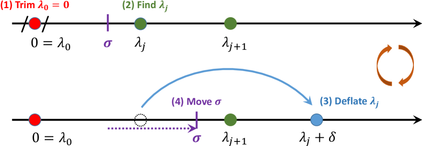
Algorithm 2, called iSIRA, summarizes the SIRA method combined with techniques of trimming (Section 2.1) and deflation (Section 2.2) for finding some smallest positive eigenvalues and associated eigenvectors of the GLEP (2.1). The techniques of trimming, deflation and shift-invert enhance can be described as in the Figure 1.

Figure 1: (1) Trim $\lambda_{0}=0$; (2) Find $\lambda_{j}\ (j>0)$; (3) Deflate $\lambda_{j}$ to $\lambda_{j}+\delta$; (4) Move $\sigma$.

Algorithm 2 iSIRA: integrated SIRA method for GLEP (2.1)

0:  An $n\times n$ graph Laplacian matrix $L$; a number of desired value $d$; an $n\times k_{0}$ column orthonormal matrix $U_{k_{0}}$, $1\leq k_{0}<m$, that each column of $U_{k_{0}}$ is also orthogonal to $\mathbf{1}_{n}$; trimmed index $1\leq i\leq n$; a deflating scalar $\delta>0$; target shift $\sigma(=0)$; tolerances $\varepsilon$; maximum dimension of the search space $m$ and the restart size of the subspace $q$. Note that $1\leq d\leq q<m\ll n$.

0:  The first $d$ smallest positive pairs $(\lambda_{j},\mathbf{v}_{j})$ of $L$, $j=1,\ldots,d$.

1:  Set $D=[\ ]$, $V=[\ ]$ (empty arrays), $k=k_{0}$ and $\text{flag}=0$.

2:  for $j=1,\ldots,d$ do

3:     while $\text{flag}=0$ do

4:        Compute $W_{k}=(L+\delta VV^{\top})U_{k}$ and $H_{k}=U_{k}^{\top}W_{k}$.

5:        % Subspace Extraction

6:        Compute all eigenpairs of $H_{k}$, say $\{(\theta_{1},\mathbf{s}_{1}),\ldots,(\theta_{k},\mathbf{s}_{k})\}$, where $\theta_{t}$ is in ascending order and $\|\mathbf{s}_{t}\|_{2}=1$, $t=1,\ldots,k$. Denote $S_{k}=[\mathbf{s}_{1}\ \cdots\ \mathbf{s}_{k}]$.

7:        Compute the residual $\mathbf{r}=W_{k}\mathbf{s}_{1}-\theta_{1}U_{k}\mathbf{s}_{1}$.

8:        if $\|\mathbf{r}\|_{2}<\varepsilon$ then

9:           Update $D=[D\ \ \lambda_{j}]$ and $V=[V\ \ \mathbf{v}_{j}]$, where $\lambda_{j}=\theta_{1}$ and $\mathbf{v}_{j}=U_{k}\mathbf{s}_{1}$.

10:           Set $\text{flag}=1$.

11:        else

12:           if $k=m$ then

13:              % Subspace Restart
$U_{k}=U_{m}S_{k}(:,1\text{{:}}q)$, $W_{k}=W_{m}S_{k}(:,1\text{{:}}q)$, $H_{k}=\text{diag}\{\theta_{1},\ldots,\theta_{q}\}$.

14:              Set $k=q$.

15:           end if

16:           % Subspace Expansion

17:           Find a solution $\mathbf{z}^{\ast}$ of (2.2) if $j=1$; of (2.14) if $j>1$.
% Singularity Trimming and Eigenvalue Deflating
(i)  Solve the linear system (2.4) if $j=1$; the system (2.15) if $j>1$.
(ii) Compute the $n$-vector $\mathbf{z}^{\ast}$ (2.5).

18:           Orthonormalize $\mathbf{z}^{\ast}$ against $U_{k}$ (and $V$ if $j>1$) to obtain $\mathbf{u}$.

19:           Expand $U_{k}$ by $U_{k+1}=\big{[}U_{k}\ \ \mathbf{u}\big{]}$. Set $k=k+1$.

20:        end if

21:     end while

22:     % Eigenvector Purging
$U_{k}=U_{k}S_{k}(:,2\text{{:}}k)$, $W_{k}=W_{k}S_{k}(:,2\text{{:}}k)$, $H_{k}=\text{diag}\{\theta_{2},\ldots,\theta_{k}\}$.

23:     Move $\sigma\approx\theta_{2}$. Set $k=k-1$ and $\text{flag}=0$.

24:  end for

For a given $k\geq 1$, as in line 6 of the iSIRA algorithm, let $U_{k}$ be the current searching subspace and $\{(\theta_{1},\mathbf{s}_{1}),\cdots,(\theta_{k},\mathbf{s}_{k})\}$ be the set of eigenpairs of $H_{k}$ with the ascending order of eigenvalues and the unit norm of each eigenvector. The $k\times k$ column orthonormal matrix $S_{k}=\begin{bmatrix}\mathbf{s}_{1}&\cdots&\mathbf{s}_{k}\end{bmatrix}$ is the collection of the eigenvectors of $H_{k}$.

We first explain the step – subspace restart – in line 12 to 15 of the iSIRA algorithm. Due to the storage requirements and computational costs, the order of the searching subspace $k$ can not be too large and shall be limited. That is to say, we have to shrink down the subspace in case the dimension is equal to the limit size $m$. This process is called restart. So, once we generate an $m$-dimension search space $U_{m}$, i.e. $k=m$, we will reduce $U_{m}$ to a $q$-dimensional matrix, $1\leq q<m$, that preserves some useful information. To maintain the first $q$ eigeninformation, the matrices $U_{m}$, $W_{m}$ and $H_{m}$ in the iSIRA will be updated by

$$U_{k}\leftarrow U_{m}S_{m}(:,1\text{{:}}q),\ W_{k}\leftarrow W_{m}S_{m}(:,1\text{{:}}q),\ H_{k}\leftarrow\text{{diag}}\{\theta_{1},\ldots,\theta_{q}\},\ k\leftarrow q.$$

We then discuss the step – eigenvector purging – in line 22 of the iSIRA algorithm. Suppose we have a convergent eigenpair $(\lambda_{j},\mathbf{v}_{j})$ for some $1\leq j\leq d$, where $\lambda_{j}=\theta_{1}$ and $\mathbf{v}_{j}=U_{k}\mathbf{s}_{1}$. The deflating action will throw $\lambda_{j}$ forward to $\lambda_{j}+\delta$, and the operation matrix will, for the subsequent loops, contain the deflating term $L+\delta\mathbf{v}_{j}\mathbf{v}_{j}^{\top}$. See Section 2.2 and line 17 of the iSIRA algorithm. Furthermore, we can also in fact purge the direction of $\mathbf{v}_{j}=U_{k}\mathbf{s}_{1}$. Consequently, owing to $U_{k}^{\top}U_{k}=I_{k}=S_{k}^{\top}S_{k}$, we will update $U_{k}$, $W_{k}$ and $H_{k}$ as follows

$$U_{k}\leftarrow U_{k}S_{k}(:,2\text{{:}}k),\ W_{k}\leftarrow W_{k}S_{k}(:,2\text{{:}}k),\ H_{k}\leftarrow\text{{diag}}\{\theta_{2},\ldots,\theta_{k}\},\ k\leftarrow k-1,$$

which are the modifications in line 22 of the iSIRA algorithm. Note that, in this case, the dimension of the searching subspace is shrunk to $k-1$.

4 Numerical Experiments

In this section, we demonstrate the efficiency and accuracy of the iSIRA algorithm (Algorithm 2), to solve the GLEP (2.1) for computing some smallest positive eigenvalues and associated eigenvectors. We use isira, Integrated SIRA, to denote Algorithm 2.

All computations in this section are carried out in MATLAB 2017a. For the hardware configuration, we use a DELL XPS 15 9560 laptop with an Intel i7-7700HQ Quad Core, 16GB RAM, and the Windows 10 operating system. The data sets to our numerical experiments are provided within KONECT [17] (Koblenz Network Collection, http://konect.uni-koblenz.de) and we consider the undirected, unweighted networks.

Moreover, to demonstrate the performance of our algorithm, we compare isira with two methods. We call the MATLAB built-in function eigs to compute the eigenvalues with smallest magnitudes using the diagonal perturbation $\tau I_{n}$, where $\tau>0$ is a small perturbation such as $10^{-8}$ and $n$ is the amount of vertex. Note that we have to compute $11$ eigenvalues of $L_{\tau}:=L+\tau I_{n}$ since the smallest one is equal to $\tau$.

Beside, we also apply the idea of null-space deflation in [11], proposed by the part authors (Huang, Lin and Yau) of this paper, to the graph Laplacian matrix. In short, using a rank-two correction, the matrix $L$ is transformed to $L_{d}+\big{[}\mathbf{e}_{1}\ \mathbf{1}_{n}\big{]}\Big{[}{-\mathbf{e}_{1}^{\top}\atop\mathbf{1}_{n}^{\top}}\Big{]}$, where $L_{d}:=L+\mathbf{e}_{1}\mathbf{e}_{1}^{\top}$. Note that this method is based on the eigs algorithm with the deflation of the zero eigenvalue and we call it as ndeigs (Null-space Deflating eigs). That is, we calculate some smallest positive eigenvalues using eigs with a function handle specified how to solve the linear systems whose the coefficient matrix $L_{d}$ together with a rank-two correction.

As a consequence, these two methods need to compute the matrix factorizations of $L_{\tau}$ and $L_{d}$ in advance for solving the linear systems involved in eigs. Moreover, the convergence tolerance of each eigensolver is set to be $10^{-8}$.

Remark 4.1.

We give some remarks on the trimming index and the deflating coefficient indicated in Section 2.1 and Section 2.2, respectively.

• The choice of trimming index may be a hyperparameter. In practice, we select the one whose diagonal entry has the maximum degree so that there are more rows (columns) will has strictly diagonally dominant property. In Example 4.2, we will present some comparison results.

• We choose $\delta=2\cdot\max\{\text{diag}(L)\}$ to be the deflating coefficient in Theorem 2.5 based on the Gershgorin Theorem [9]. This can ensure that deflating eigenvalues will not fall inside the spectrum of $L$ and still keep the order of magnitude.

Example 4.1.

We compute the first ten smallest eigenvalues of the networks from KONECT with vertex size larger than 100,000. The first five data in Table 1 are connected networks and the rest of networks have more than one connected component. For the latter, we first identify which component of each vertex in the graph belongs to and then take out the subnetwork that has the most members.

Code	$n$	$nnz$	Time (sec)
			isira	ndeigs	eigs
LM	104,103	4,490,269	$72.3$	$153.4$	$1856.0$
GW	196,591	2,097,245	$51.6$	$61.3$	$224.7$
CA	334,863	2,186,607	$66.8$	$67.6$	$203.3$
CY	1,134,890	7,110,138	$315.3$	—	—
HY	1,402,673	6,957,511	$223.3$	—	—
FX	2,523,386	18,360,988	$740.4$	—	—
FI	105,722	4,739,058	$54.8$	$61.6$	$404.7$
SK	1,694,616	23,883,034	$660.6$	$10310.5$	—
YT	3,216,075	21,955,823	$1068.0$	—	—

Table 1: The CPU time of the eigensolvers for networks. The symbol — means that 16 GB memory was not enough for computing the required matrix factorizations. The first column is the code name assigned in KONECT. $n$ shows the vertex size of the (largest) connected network. The column $nnz$ denotes the number of nonzero elements of its Laplacian matrix and the last column records the time costs of the three methods.

(a) Sparse Pattern of FX

(b) Residual Evolution of FX

(c) Sparse Pattern of YT

(d) Residual Evolution of YT

Figure 2: Sparsity patterns of the reverse Cuthill-McKee ordering and convergence histories of the isira method for the networks FX and YT.

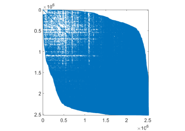
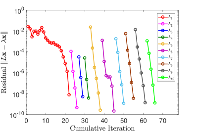
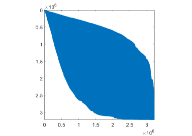
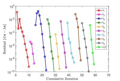
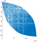
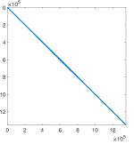
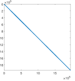
For large networks whose bandwidth are very wide after performing the reordering such the minimum degree algorithm [20], Cuthill-McKee algorithm [6] and the reverse Cuthill-McKee algorithm[8], to achieve the matrix factorizations will suffer from the problem on out of memory. Figure 2 shows matrix pattern of FX and YT after performing the reverse Cuthill-McKee algorithm. As we can see that the sparse pattern is still very “fat”and this will make the factorization produce dense matrices. In such situations, the isira method circumvent this difficulty using the iterative method and inexactly solving the linear systems contained the eigensolver.

Table 1 reveals feasibility of isira to capture some smallest eigenvalues in a reasonable time cost. All networks have similar convergence processes and we present iteration behaviors of FX and YT in Figure 2. Moreover, in Table 1, we also see that the techniques from our previous method ndeigs [11] can adjust the structure of a matrix without changing its sparsity of the matrix. This can reduce possibility of zero diagonal elements appearing in the execution of the matrix factorization. We will demonstrate this effect again in Remark 4.2.

Example 4.2.

In Remark 4.1, we make some interpretable idea to select the vertex whose degree is the maximum as the trimming index. Table 2 shows some comparisons between the vertex degree and the computational time.

CY		HY		FX		YT		SK
degree	time	degree	time	degree	time	degree	time	degree	time
1	406.6	1	319.2	1	784.5	1	1462.2	1	820.1
29	360.0	172	262.0	57	744.5	29	1379.3	360	747.6
28,754	315.3	31,883	223.3	1,474	740.4	91,751	1068.0	35,455	660.0

Table 2: The CPU time of the isira method using different trimming indices.

In the first four examples, the third row is exact the index $n$, the fourth row presents the results by deleting the first row and column, and the last row is obtained by trimming the vertex which has the maximum degree. In the case of SK, the minimum degree is still equal to one but is not equal to the last index. The last row also picks the index with the maximum degree. The value 360 in the network SK is the degree of its first vertex. On our experimental experience, trimming the vertex with the smallest degree always get slower computational efficiency. This may indirectly display that trimming the index of the vertex with the maximum degree may be an appropriate choice.

(a) WO

(b) CD

(c) RD

(d) R1

(e) RO

Figure 3: Networks in Table 3 have narrower bandwidth patterns after reordering.

Code	$n$	$nnz$	Time (sec)
			ndeigs	eigs
WO	145,145	1,457,605	$15.3$	$31.2$
CD	317,080	2,416,812	$76.6$	$249.5$
RD	1,087,562	4,170,590	$8.0$	$9.6$
R1	1,351,137	5,109,539	$8.0$	$11.7$
RO	1,957,027	7,477,803	$11.9$	$16.9$

Table 3: The CPU time of the eigs and ndeigs for networks having thinner bandwidth after the index permutation as shown in Figure 3. The contents of the first row of this table are as introduced in Table 1.

Remark 4.2.

The isira is committed to solve the GLEP whose network pattern is wide even after suitable reordering of vertices. That is, in this case, the graph Laplacian matrix has no LU factorization available. On the contrary, if the bandwidth of a matrix becomes narrow after applying some reordering algorithms, then the LU factorization is very “cheap” either on the demand of memory or the time of computing. Under such situations, eigs and ndeigs become preferable since the inner linear systems can be solved by the LU factorization.

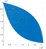
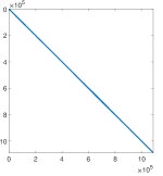
Figure 3 gives five examples that the matrices have narrower bandwidth patterns after performing the reverse Cuthill-McKee algorithm (the MATLAB built-in function: symrcm). Tale 3 presents the information of these networks and the time cost of eigs and ndeigs methods. It is worth to mention that the rank-two correction strategy in ndeigs [11], our previous method, makes the performance be superior to eigs.

5 Conclusions and Future Works

Graph Laplacian eigenvalue problems focus on the extraction of potential quantities, such as eigenvalues and eigenvectors of network structures. Due to the graph Laplacian matrix, generated from a simple, connected and undirected graph, is symmetric positive semi-definite and the information what we are interested often be hidden in the eigenvalues with small magnitude. This indicates that we have to address the problem of solving a singular system. Thus, the study of efficient eigensolvers for finding some smallest positive eigenvalues and associated eigenvectors of the graph Laplacian eigenvalue problem is a challenging and important topic.

To this end, based on the method of inexact shift-invert residual Arnoldi (SIRA) [18, 19], we derive a trimming technique in Section 2.1 to implicitly remedy the singularity of the graph Laplacian matrix and get a solution which is orthogonal to the null space for expanding the searching subspace. Furthermore, we apply the deflating approach to exclude the influence of convergence eigenvalues so as to focus on capturing the smallest positive one and detect a few desired eigenvalues in order. Numerical experiments show that, compared with the numerical implementations of traditional diagonal perturbation eigs and the null-space deflation eigensolver ndeigs [11] using direct methods for inner linear systems, the new derived algorithm iSIRA, integrated SIRA (SIRA with trimming and deflating techniques), reveals more efficient and feasible when a LU factorization of the graph Laplacian matrix is not available.

According to the concise algorithm of SIRA, in the future, we will focus on the development a GPU version of the iSIRA algorithm (Algorithm 2). In addition, we will pay attention to Laplacian matrix arising from a direct graph. Note that in such a case, all properties and advantages of a undirect Laplacian proposed in this paper are no longer be applied. How to explore new features and develop a fast eigensolver is under investigation.

6 Acknowledgments

The first three authors would like to thank the grant support from the Ministry of Science and Technology in Taiwan, and the ST Yau Center and Big Data Research at the National Chiao Tung University. The first and the third authors would further thank Dr. Pin-Yu Chen at IBM’s T.J. Watson Research Center for proving application information about this topic.

References

- [1] A. Arenas, A. D az-Guilera, J. Kurths, Y. Moreno, and C. Zhou. Synchronization in complex networks. Phys. Rep., 469(3):93–153, 2008.
- [2] Z. Bai, J. Demmel, J. Dongarra, A. Ruhe, and H. van der Vorst. Templates for the Solution of Algebraic Eigenvalue Problems: A Practical Guide. SIAM: Society for Industrial and Applied Mathematics, Philadelphia, PA, 2000.
- [3] M. Belkin and P. Niyogi. Laplacian eigenmaps for dimensionality reduction and data representation. Neural Comput., 15(6):1373–1396, 2003.
- [4] P. Y. Chen and A. O. Hero. Deep community detection. IEEE Tr. Signal Proces., 63(21):5706–5719, Nov 2015.
- [5] P. Y. Chen and A. O. Hero. Phase transitions in spectral community detection of large noisy networks. In 2015 IEEE International Conference on Acoustics, Speech and Signal Processing (ICASSP), pages 3402–3406, April 2015.
- [6] E. Cuthill and J. McKee. Reducing the bandwidth of sparse symmetric matrices. In Proceedings of the 1969 24th National Conference, ACM ’69, pages 157–172, New York, NY, USA, 1969. ACM.
- [7] S. Fortunato. Community detection in graphs. Phys. Rep., 486(3):75–174, 2010.
- [8] N. E. Gibbs. Algorithm 509: A hybrid profile reduction algorithm [F1]. ACM Trans. Math. Softw., 2(4):378–387, Dec. 1976.
- [9] G. H. Golub and C. F. Van Loan. Matrix Computations. The Johns Hopkins University Press, Baltimore, MD, 4th edition, 2012.
- [10] T.-M. Huang, H.-E. Hsieh, W.-W. Lin, and W. Wang. Eigenvalue solvers for three dimensional photonic crystals with face-centered cubic lattice. J. Comput. Appl. Math., 272:350 – 361, 2014.
- [11] W.-Q. Huang, X. D. Gu, W.-W. Lin, and S.-T. Yau. A novel symmetric skew-Hamiltonian isotropic Lanczos algorithm for spectral conformal parameterizations. J Sci. Comput., 61(3):558–583, Dec 2014.
- [12] I. C. F. Ipsen. Computing an eigenvector with inverse iteration. SIAM Rev., 39(2):254–291, 1997.
- [13] Z. Jia and C. Li. Inner iterations in the shift-invert residual Arnoldi method and the Jacobi-Davidson method. Sci. China Math., 57(8):1733–1752, 2014.
- [14] J. A. Kelner, L. Orecchia, A. Sidford, and Z. A. Zhu. A simple, combinatorial algorithm for solving sdd systems in nearly-linear time. In Proceedings of the Forty-fifth Annual ACM Symposium on Theory of Computing, STOC ’13, pages 911–920, New York, NY, USA, 2013. ACM.
- [15] I. Koutis, G. L. Miller, and R. Peng. A nearly-m log n time solver for SDD linear systems. In 2011 IEEE 52nd Annual Symposium on Foundations of Computer Science, pages 590–598, Oct 2011.
- [16] I. Koutis, G. L. Miller, and D. Tolliver. Combinatorial preconditioners and multilevel solvers for problems in computer vision and image processing. Comput. Vis. Image. Und., 115(12):1638–1646, 2011. Special issue on Optimization for Vision, Graphics and Medical Imaging: Theory and Applications.
- [17] J. Kunegis. Konect: The Koblenz Network Collection. In Proceedings of the 22nd International Conference on World Wide Web, WWW ’13 Companion, pages 1343–1350, New York, NY, USA, 2013. ACM.
- [18] C.-R. Lee. Residual Arnoldi method: theory, package and experiments. PhD thesis, Department of Computer Science,University of Maryland at College Park, 2007.
- [19] C.-R. Lee and G. W. Stewart. Analysis of the residual Arnoldi method. Technical report, Department of Computer Science,University of Maryland at College Park, 2007.
- [20] H. M. Markowitz. The elimination form of the inverse and its application to linear programming. Manage. Sci., 3(3):255–269, 1957.
- [21] B. Mohar. Some applications of Laplace eigenvalues of graphs, pages 225–275. Springer Netherlands, Dordrecht, 1997.
- [22] B. Mohar and S. Poljak. Eigenvalues in Combinatorial Optimization, pages 107–151. Springer New York, New York, NY, 1993.
- [23] J. J. Molitierno. Applications of combinatorial matrix theory to Laplacian matrices of graphs. Discrete Mathematics and Its Applications. CRC Press, Boca Raton, Florida, 2012.
- [24] M. E. J. Newman. Finding community structure in networks using the eigenvectors of matrices. Phys. Rev. E, 74:036104, Sep 2006.
- [25] A. Y. Ng. Feature selection, L1 vs. L2 regularization, and rotational invariance. In Proceedings of the Twenty-first International Conference on Machine Learning, ICML ’04, pages 78–, New York, NY, USA, 2004. ACM.
- [26] A. Y. Ng, M. I. Jordan, and Y. Weiss. On spectral clustering: Analysis and an algorithm. In T. G. Dietterich, S. Becker, and Z. Ghahramani, editors, Advances in Neural Information Processing Systems 14, pages 849–856. MIT Press, 2002.
- [27] J. Pang, G. Cheung, A. Ortega, and O. C. Au. Optimal graph laplacian regularization for natural image denoising. In 2015 IEEE International Conference on Acoustics, Speech and Signal Processing (ICASSP), pages 2294–2298, April 2015.
- [28] B. N. Parlett. The Symmetric Eigenvalue Problem. SIAM: Society for Industrial and Applied Mathematics, 1998.
- [29] Z. Qu. Cooperative Control of Dynamical Systems: Applications to Autonomous Vehicles. Springer-Verlag, 2009.
- [30] S. E. Schaeffer. Graph clustering. Comput. Sci. Rev., 1(1):27–64, 2007.
- [31] J. Shi and J. Malik. Normalized cuts and image segmentation. IEEE T. Pattern Anal., 22(8):888–905, Aug 2000.
- [32] D. A. Spielman and S.-H. Teng. Nearly-linear time algorithms for graph partitioning, graph sparsification, and solving linear systems. In Proceeding STOC ’04 Proceedings of the thirty-sixth annual ACM symposium on Theory of computing, pages 81–90, New York, NY, USA, 2004. ACM.
- [33] D. A. Spielman and S.-H. Teng. Nearly linear time algorithms for preconditioning and solving symmetric, diagonally dominant linear systems. SIAM J. Matrix. Anal. A., 35(3):835–885, 2014.
- [34] G. W. Stewart. Matrix Algorithms: Volume II: Eigensystems. SIAM: Society for Industrial and Applied Mathematics, 2001.
- [35] A. N. Tikhonov and V. t. V. Y. Arsenin. Solutions of ill posed problems. V. H. Winston & Sons, Washington, D.C.: Winston, 1977.
- [36] P. M. Vaidya. Solving linear equations with symmetric diagonally dominant matrices by constructing good preconditioners. A talk based on this manuscript, 2(3.4):2–4, 1991.
- [37] U. von Luxburg. A tutorial on spectral clustering. Stat. Comput., 17(4):395–416, Dec 2007.
- [38] S. White and P. Smyth. A Spectral Clustering Approach to Finding Communities in Graphs, pages 274–285. Proceedings of the 2005 SIAM International Conference on Data Mining. 2005.
- [39] R. Xu and D. Wunsch. Survey of clustering algorithms. IEEE T. Neural Networ., 16(3):645–678, May 2005.