Image-domain multi-material decomposition for dual-energy CT based on correlation and sparsity of material images

Abstract

Purpose: Dual energy CT (DECT) enhances tissue characterization because it can produce images of basis materials such as soft-tissue and bone. DECT is of great interest in applications to medical imaging, security inspection and nondestructive testing. Theoretically, two materials with different linear attenuation coefficients can be accurately reconstructed using DECT technique. However, the ability to reconstruct three or more basis materials is clinically and industrially important. Under the assumption that there are at most three materials in each pixel, there are a few methods that estimate multiple material images from DECT measurements by enforcing sum-to-one and a box constraint ([0 1]) derived from both the volume and mass conservation assumption. The recently proposed image-domain multi-material decomposition (MMD) method introduces edge-preserving regularization for each material image which neglects the relations among material images, and enforced the assumption that there are at most three materials in each pixel using a time-consuming loop over all possible material-triplet in each iteration of optimizing its cost function. We propose a new image-domain MMD method for DECT that considers the prior information that different material images have common edges and encourages sparsity of material composition in each pixel using regularization.

Method: The proposed PWLS-TNV-$\ell_{0}$ method uses penalized weighted least-square (PWLS) reconstruction with three regularization terms. The first term is a total nuclear norm (TNV) that accounts for the image property that basis material images share common or complementary boundaries and each material image is piecewise constant. The second term is a $\ell_{0}$ norm that encourages each pixel containing a small subset of material types out of several possible materials. The third term is a characteristic function based on sum-to-one and box constraint derived from the volume and mass conservation assumption. We apply the Alternating Direction Method of Multipliers (ADMM) to optimize the cost function of the PWLS-TNV-$\ell_{0}$ method.

Result: We evaluated the proposed method on a simulated digital phantom, Catphan©600 phantom and patient’s pelvis data. We implemented two existing image-domain MMD methods for DECT, the Direct Inversion mendonca2014a and the PWLS-EP-LOOP method xue2017statistical . We initialized the PWLS-TNV-$\ell_{0}$ method and the PWLS-EP-LOOP method with the results of the Direct Inversion method and compared performance of the proposed method with that of the PWLS-EP-LOOP method. The proposed method lowered bias of decomposed material fractions by $84.47\%$ in the digital phantom study, by $99.50\%$ in the Catphan©600 phantom study, and by $99.64\%$ in the pelvis patient study, respectively, compared to the PWLS-EP-LOOP method. The proposed method reduced noise standard deviation (STD) by $52.21\%$ in the Catphan©600 phantom study, and by $16.74\%$ in the patient’s pelvis study, compared to the PWLS-EP-LOOP method. The proposed method increased volume fraction accuracy by $6.04\%,20.55\%$ and $13.46\%$ for the digital phantom, the Catphan©600 phantom and the patient’s pelvis study, respectively, compared to the PWLS-EP-LOOP method. Compared with the PWLS-EP-LOOP method, the root mean square percentage error (RMSE($\%$)) of electron densities in the Catphan©600 phantom was decreased about $7.39\%$.

Conclusions: We proposed an image-domain MMD method, PWLS-TNV-$\ell_{0}$, for DECT. PWLS-TNV-$\ell_{0}$ method takes low rank property of material image gradients, sparsity of material composition and mass and volume conservation into consideration. The proposed method suppresses noise, reduces crosstalk, and improves accuracy in the decomposed material images, compared to the PWLS-EP-LOOP method.

keywords: Dual energy CT (DECT), Spectral CT, Multi-material decomposition (MMD), Total nuclear norm (TNV), Penalized weighted least-square (PWLS)

I Introduction

Dual energy CT (DECT) enhances tissue characterization which is of great interest in applications of medical imaging, security inspection and nondestructive testing. In principle, with DECT measurements acquired at low and high energies only two basis materials can be accurately reconstructed niu2014iterative ; alvarez1976energy ; alvarez1977x ; macovski1976energy ; marshall1981initial ; stonestrom1981framework . In reality a scanned object often contains multiple basis materials and many clinical and industrial applications desire multi-material images laidevant2010compositional ; liu2009quantitative . A natural thought is to utilize spectral CT that acquires multi-energy measurements to achieve multiple basis material images. However, spectral CT requires either multiple scans which results in high radiation to patients and needs complex processing (e.g., registration) of CT images at different energies liu2016ticmr , or specialized scanners which are expensive and not available clinically yet, such as energy-sensitive photon-counting detectors bornefalk2010photon ; gao2011multi ; shikhaliev2011photon ; ding2014high ; li2015spectral . In this work, we focus on multi-material decomposition (MMD) using DECT measurements obtained from commercial available conventional DECT scanners.

Multi-material decomposition from DECT measurements is an ill-posed problem since multiple sets of images are estimated from two sets of measurements associated with low and high energies. Several methods have been proposed to reconstruct multi-material images from DECT measurements mendonca2014a ; lamb2015stratification ; long2014multi-material ; xue2017statistical . Mendonca et al. mendonca2014a proposed an image-domain MMD method that decomposes FBP images at low- and high-energy reconstructed from a DECT scan into multiple images of basis materials. This method uses a material triplet library (e.g., blood-air-fat, fat-blood-contrast agent), finds the optimal material triplet for each pixel, and then decompose each pixel into the basis materials that correspond to the best material triplet. It uses mass and volume conservation assumption, and a constraint that each pixel contains at most three materials out of several possible materials to help solve the ill-posed problem of estimating multiple images from DECT measurements. The decomposed multiple material images by this method have been successfully applied to applications of virtual non-contrast-enhanced (VNC) images, fatty liver disease, and liver fibrosis mendonca2014a ; lamb2015stratification . However, this method estimates volume fractions of basis materials from linear attenuation coefficient (LAC) pairs at high and low energies pixel by pixel without considering the noise statistics of DECT measurements and prior information of material images, such as piecewise constant property of material images and similarity between different material images. Using similar constraints that help estimating multiple material images from DECT scans, Long and Fessler long2014multi-material proposed a penalized-likelihood (PL) method with edge-preserving for each material to directly reconstruct multiple basis material images from DECT measurements. This PL method significantly reduced noise, streak and cross-talk artifacts in the reconstructed basis material images. However, this PL method is computationally expensive mainly due to the forward and back-projection between multiple material images and DECT sinograms at low and high energies. Xue et al. xue2017statistical proposed a statistical image-domain MMD method that uses penalized weighted least-square (PWLS) estimation with edge-preserving (EP) regularizers for each material. We call this method the PWLS-EP-LOOP method hereafter. Compared to the image-domain direct inversion method in mendonca2014a , the PWLS-EP-LOOP method reduces noise and improves the accuracy of decomposed volume fractions. Because it is an image-domain method without forward and back-projection, it is computationally more practical than the PL method. To enforce sum-to-one and a box constraint $([0,1])$ derived from both volume and mass conservation assumption mendonca2014a ; long2014multi-material , the aforementioned three methods loop over material triples in a material triplet library formed from several basis materials of interest, and uses a criterion to determine the optimal material triplet for each pixel. Without considering the prior information that different material images have common edges, the edge-preserving regularization of the PL and PWLS-EP-LOOP method is imposed on each material image.

In this paper, we propose a PWLS-TNV-$\ell_{0}$ method whose cost function consists of a weighted least square data term and three regularization terms. The first term is total nuclear norm (TNV) regularization derived from image property that basis material images share common or complementary boundaries. The second term is a $\ell_{0}$ norm that encourages each pixel containing a small subset of material types out of several possible materials and each material image is piecewise constant. The third term is a characteristic function based on sum-to-one and a box constraint accounting for the volume and mass conservation assumption. We apply the Alternating Direction Method of Multipliers method (ADMM, also known as split Bregman method goldstein2009the ) to solve the optimization problem of the PWLS-TNV-$\ell_{0}$ method. We solve the subproblems of ADMM for the PWLS-TNV-$\ell_{0}$ method using Conjugate Gradient(CG), Singular Value Thresholding (SVT) cai2010singular , Hard Thresholding (HT) blumensath2008iterative ; Trzasko2007Sparse and projection onto convex sets. We evaluate the proposed PWLS-TNV-$\ell_{0}$ method on simulated digital phantom, Catphan©600 phantom and patient data, and results demonstrate that the proposed method suppresses noise, decreases crosstalk and improves accuracy in decomposed material images, compared to the PWLS-EP-LOOP method.

This paper is organized as follows. Section II describes the PWLS-TNV-$\ell_{0}$ method and the ADMM algorithm that minimizes its cost function. Section III presents experiments and results. Section IV discusses the propose models and future work. Finally, we draw our conclusions in Section V.

II Method

II.1 DECT model

For dual energy CT, we can obtain a two-channel image $\bm{y}=(\bm{y}^{T}_{H},\bm{y}^{T}_{L})^{T}\in\mathbb{R}^{2N_{p}}$, where $\bm{y}_{H},\bm{y}_{L}\in\mathbb{R}^{N_{p}}$ are attenuation images at high- and low-energy respectively and $N_{p}$ is the number of pixels. With mass and volume conservation assumption mendonca2014a , the spatially- and energy-dependent attenuation image $\bm{y}$ satisfy

$$\left(\begin{array}[]{ccc}\bm{y}_{H}\\ \bm{y}_{L}\end{array}\right)=\left(\begin{array}[]{ccc}\sum_{l=1}^{L_{0}}\mu_{lH}\bm{x}_{l}\\ \sum_{l=1}^{L_{0}}\mu_{lL}\bm{x}_{l}\end{array}\right),$$ (5)

where $\mu_{lH}$ and $\mu_{lL}$ denote the linear attenuation coefficient of the $l$-th material at the high- and low-energy respectively, $\bm{x}_{l}=(x_{l1},x_{l2},...,x_{ln},...,x_{lN_{p}})\in\mathbb{R}^{N_{p}}$ denotes the volume fraction of the $l$-th material and $L_{0}$ is the number of materials. According to volume conservation, the volume fraction $\bm{x}=(\bm{x}^{T}_{1},\bm{x}^{T}_{2},\ldots,\bm{x}^{T}_{L_{0}})^{T}\in\mathbb{R}^{L_{0}N_{P}}$ satisfies sum-to-one and box constraints,

$$\left\{\begin{array}[]{ccc}\sum\limits_{l=1}^{L_{0}}x_{lj}=1,\quad\forall j\\ 0\leq x_{lj}\leq 1,\quad\forall l,j.\end{array}\right.$$ (8)

We rewrite (5) in the matrix form as

$$\bm{y}=\bm{A}\bm{x},$$ (9)

where $\bm{A}\in\mathbb{R}^{2N_{p}\times L_{0}N_{p}}$ is

$$\bm{A}=\bm{A}_{0}\otimes\bm{I}_{N_{p}}.$$ (10)

Here, $\otimes$ denotes the Kronecker producter. $\bm{A}_{0}$ is the material composition matrix

$$\bm{A}_{0}=\left(\begin{array}[]{ccc}\mu_{1H}&\mu_{2H}\cdots\mu_{L_{0}H}\\ \mu_{1L}&\mu_{2L}\cdots\mu_{L_{0}L}\end{array}\right),$$ (13)

and $\bm{I}_{N_{p}}$ is the $N_{p}\times N_{p}$ identity matrix. In this paper, we obtain $\mu_{lH}$, $\mu_{lL}$ by the same method in szczykutowicz2010dual ; granton2008implementation ; niu2014iterative . Firstly, we manually select two uniform regions of interest (ROIs) in the CT images that contain the $l$-th basis material. Then, we compute the average CT values in the two ROIs as $\mu_{lH}$ and $\mu_{lL}$ of the decomposition matrix $\bm{A}_{0}$ .

II.2 Variational model

In practice the acquired attenuation image $\bm{y}$ is corrupted with noise, i.e.,

$$\bm{y}=\bm{A}\bm{x}+\bm{\varepsilon},$$ (14)

where $\bm{\varepsilon}\in\mathbb{R}^{2N_{p}}$ is assumed to be additive white noise, i.e.,

$$\bm{\varepsilon}\sim N(\bm{0},\Sigma)$$ (15)

where $\bm{0}$ is the zero vector in $\mathbb{R}^{2N_{p}}$ and $\Sigma$ is the covariance matrix of $\bm{\varepsilon}$.

We propose to use a penalized weighted least-square (PWLS) method to estimate multi-material images $\bm{x}$ from DECT images $\bm{y}$. The probability density function (pdf) of $\bm{y}$ is

$$p(\bm{y}|\bm{x})$$

$$= \frac{1}{(2\pi)^{N_{p}}|\Sigma|^{\frac{1}{2}}}\exp{(-\frac{(\bm{y}-\bm{A}\bm{x})^{T}\Sigma^{-1}(\bm{y}-\bm{A}\bm{x})}{2})}.$$ (16)

According to maximum-likelihood (ML) estimate, the negative log-likelihood is,

$$\bar{L}(\bm{x}) =\frac{1}{2}\|\bm{y}-\bm{A}\bm{x}\|_{\Sigma^{-1}}^{2}.$$ (17)

We assume the noise in each pixel is uncorrelated and every pixel in the high- or low-energy CT image has the same noise variance as in our pervious work niu2014iterative ; xue2017statistical , i.e.,

$$\Sigma=\mathrm{diag}(\sigma_{H}^{2}\bm{I}_{N_{p}},\sigma_{L}^{2}\bm{I}_{N_{p}}),$$ (18)

where $\sigma_{H}^{2}$ and $\sigma_{L}^{2}$ are the noise variance for the high-energy CT image $\bm{y}_{H}$ and low-energy image $\bm{y}_{L}$ respectively. To estimate $\sigma_{H}^{2}$ and $\sigma_{L}^{2}$ we select a homogeneous region with a single material in the high- and low-energy image and calculate their numerical variances respectively.

The PWLS problem that estimates fraction images $\bm{x}$ from noisy DECT images $\bm{y}$ takes the following form

$$\hat{\bm{x}}=\arg\min_{\bm{x}}\Psi(\bm{x}),\quad\Psi({\bm{x}})\ \triangleq\ \bar{L}(\bm{x})+R(\bm{x}).$$ (19)

We propose to use the following regularization term $R(\bm{x})$

$$R(\bm{x})=\beta_{1}R_{1}(\bm{x})+\beta_{2}R_{2}(\bm{x})+R_{3}(\bm{x}),$$ (20)

where the parameters $\beta_{1}$ and $\beta_{2}$ control the noise and resolution tradeoff, $R_{1}(\bm{x})$ is a total nuclear norm (TNV), $R_{2}(\bm{x})$ is a $\ell_{0}$ norm and $R_{3}(\bm{x})$ is a characteristic function based on sum-to-one and box constraints in (8). The three regularization terms will be explained in Section II.2.1, II.2.2 and II.2.3 respectively.

II.2.1 Low rankness of image gradients

The first regularization term $R_{1}(\bm{x})$ is designed to describe the correlation of material images. In practice, each region of an object typically contains several materials, and the material images share similar or complementary boundary structures. When a region contains more than one material, the fraction images of these materials share similar structure information. Structure information of an image can be captured by the image gradient. Thus, we can use the correlation of image gradient among different material images. This is realized by imposing low rankness of the generalized gradient matrix at each pixel location, for which we use total nuclear variation (TNV) as a regularization. This regularization form was previously proposed in rigie2014ageneralized ; rigie2015joint and the sum of the nuclear norm of Jacobian matrix of multi-channel image were penalized to reconstruct color images. Here, the same idea is employed to take into account of the structure correlation of fraction images of material.

More specifically, the generalized gradient matrix $(\bm{Dx})_{j}\in\mathbb{R}^{L_{0}\times N_{d}}$ at the $j$th-pixel is defined as

$$(\bm{Dx})_{j}=\left(\begin{array}[]{cccc}(\bm{J_{1}x_{1}})_{j}&(\bm{J_{2}x_{1}})_{j}&\cdots&(\bm{J_{N_{d}}x_{1}})_{j}\\ (\bm{J_{1}x_{2}})_{j}&(\bm{J_{2}x_{2}})_{j}&\cdots&(\bm{J_{N_{d}}x_{2}})_{j}\\ \vdots&\vdots&\ddots&\vdots\\ (\bm{J_{1}x_{L_{0}}})_{j}&(\bm{J_{2}x_{L_{0}}})_{j}&\cdots&(\bm{J_{N_{d}}x_{L_{0}}})_{j}\\ \end{array}\right),$$ (25)

where $\bm{J_{d}x_{l}}$ denotes the finite difference in the $d$-th direction on the fraction image of the $l$-th material $\bm{x}_{l}$, and $N_{d}$ is the number of directions. The regularization term is written as

$$R_{1}(\bm{x})=\sum\limits_{j=1}^{N_{P}}\|(\bm{Dx})_{j}\|_{\ast}\triangleq\|\bm{Dx}\|_{\ast}\triangleq R_{TNV}(\bm{x}),$$ (26)

where $\|\cdot\|_{\ast}$ denotes the nuclear norm of the matrix. The matrix $\bm{Dx}$ can be also viewed as a 3D matrix of size $L_{0}\times N_{d}\times N_{p}$ and the nuclear norm is computed at each pixel.

II.2.2 Sparsity

The second regularization considers the number of materials at each pixel is small as locally human organs often consist of few kinds of materials and the fraction is piecewise constant. Let $\bm{x}_{j}\triangleq(x_{1j},x_{2j},\cdots,x_{L_{0}j})^{T}$ be the material fraction image vector at the $j$-th pixel. We use $\ell_{0}$ norm of the gradient of $\bm{x}$ as regularization, i.e.,

$$R_{2}(\bm{x})=\sum_{j=1}^{N_{P}}\|(\nabla\bm{x})_{j}\|_{0}=\|\nabla\bm{x}\|_{0}.$$ (27)

Here, $\nabla\bm{x}=(\nabla\bm{x}^{T}_{l},\nabla\bm{x}^{T}_{2},\cdots\nabla\bm{x}^{T}_{L_{0}})^{T}$. If the discrete gradient is computed in two directions, then $\nabla\bm{x}\in\mathbb{R}^{L_{0}N_{p}\times 2}$ and $(\nabla\bm{x})_{j}\in\mathbb{R}^{L_{0}\times 2}$.

II.2.3 Volume and mass conservation

In addition, one can assume that volume and mass of the material fraction is conserved, i.e. $x_{l}$ satisfies sum-to-one and the box constraint given in (8). The regularization term $R_{3}$ is used to account for these constraints, i.e.,

$$R_{3}(\bm{x})=\chi_{S}(\bm{x})=\begin{cases}0,\quad\bm{x}\in S\\ \infty,\quad\mathrm{else},\end{cases}$$ (28)

where $S=\{\bm{x}:\sum\limits_{l=1}^{L_{0}}x_{lj}=1,0\leq x_{lj}\leq 1,j=1,\cdots,N_{p}\}$ and $\chi_{S}(\cdot)$ is the characteristic function.

In summary, the so-called PWLS-TNV-$\ell_{0}$ variational model is written as

$$\arg\min_{\bm{x}}\frac{1}{2}\|\bm{y}-\bm{A}\bm{x}\|_{\Sigma^{-1}}^{2}+\beta_{1}\|\bm{Dx}\|_{\ast}+\beta_{2}\|\nabla\bm{x}\|_{0}+\chi_{S}(\bm{x}).$$ (29)

II.3 Optimization Method

The proposed PWLS-TNV-$\ell_{0}$ model (29) is a complex problem to solve directly due to its non-convexity, non-smoothness and multiple regularization terms. We apply the Alternating Direction Method of Multipliers (ADMM) (also known as split Bregman goldstein2009the ) algorithm to solve it. By introducing auxiliary variables $\bm{u}\in\mathbb{R}^{L_{0}\times N_{d}\times N_{p}},\bm{v}\in\mathbb{R}^{L_{0}N_{p}\times 2}$ and $\bm{w}\in\mathbb{R}^{L_{0}N_{p}}$, we acquire the following equivalent constrained problem:

$$\arg\min_{\bm{x},\bm{u},\bm{v},\bm{w}} \frac{1}{2}\|\bm{y}-\bm{A}\bm{x}\|_{\Sigma^{-1}}^{2}+\beta_{1}\|\bm{u}\|_{\ast}+\beta_{2}\|\bm{v}\|_{0}+\chi_{S}(\bm{w})$$

$$s.t.~{}~{}~{} \bm{u}=\bm{Dx},~{}~{}~{}\bm{v}=\nabla\bm{x},~{}~{}~{}\bm{w}=\bm{x}.$$ (30)

To simplify, problem (30) can be formulated as the following general form

$$\arg\min_{\bm{x},\bm{z}}\bar{L}(\bm{x})+R(\bm{z})~{}~{}s.t.~{}~{}\bm{z}=\bm{Kx}$$ (31)

where $\bm{z}\triangleq(\bm{u},\bm{v},\bm{w})^{T},\bm{K}\triangleq(\bm{D},\bm{\nabla},\bm{I})^{T}.$ Here, the variables are understood in vector form and the transformation are considered as operators. The ADMM scheme for solving (31) alternates between optimizing $\bm{x}$ and $\bm{z}$ and updating the dual variable $\bm{p}$:

$$\bm{x}^{n+1} =\arg\min_{\bm{x}}\bar{L}(\bm{x})+\langle\bm{p}^{n},\bm{K}\bm{x}-\bm{z}^{n}\rangle$$

$$+\frac{\bm{\gamma}}{2}\|\bm{K}\bm{x}-\bm{z}^{n}\|^{2}_{2},$$ (32)

$$\bm{z}^{n+1} =\arg\min_{\bm{z}}R(\bm{z})+\langle\bm{p}^{n},\bm{K}\bm{x}^{n+1}-\bm{z}\rangle$$

$$+\frac{\bm{\gamma}}{2}\|\bm{K}\bm{x}^{n+1}-\bm{z}\|^{2}_{2},$$ (33)

$$\bm{p}^{n+1} =\bm{p}^{n}+\bm{\gamma}(\bm{K}\bm{x}^{n+1}-\bm{z}^{n+1}),$$ (34)

where $\bm{p}=(\bm{p}_{1},\bm{p}_{2},\bm{p}_{3})^{T}$ with $\bm{p}_{1}\in\mathbb{R}^{L_{0}\times N_{d}\times N_{p}}$, $\bm{p}_{2}\in\mathbb{R}^{L_{0}N_{p}\times 2}$ and $\bm{p}_{3}\in\mathbb{R}^{L_{0}N_{p}}$ have the same size as $\bm{D}\bm{x}$, $\bm{\nabla}\bm{x}$ and $\bm{x}$ respectively, $\langle\cdot,\cdot\rangle$ denotes inner product, and $\bm{\gamma}=(\gamma_{1},\gamma_{2},\gamma_{3})>0$ is the penalty parameters vector in (33).

In the following, we present solutions for the subproblems (32), (33) and (34). Since (32) is quadratic and differentiable on $\bm{x}$, it is equal to solve a linear system to obtain $\bm{x}^{n+1}$, i.e.,

$$G\bm{x} =\bm{A}^{T}\Sigma^{-1}\bm{y}+\bm{D}^{T}(\gamma_{1}\bm{u}^{n}-\bm{p}^{n}_{1})$$

$$+\nabla^{T}(\gamma_{2}\bm{v}^{n}-\bm{p}^{n}_{2})+\gamma_{3}\bm{w}^{n}-\bm{p}^{n}_{3},$$ (35)

where $G\bm{x}=\bm{A}^{T}\Sigma^{-1}\bm{A}\bm{x}+\gamma_{1}\bm{D}^{T}\bm{D}\bm{x}+\gamma_{2}\nabla^{T}\nabla\bm{x}+\gamma_{3}\bm{x}$. It is easy to see that this is a linear system that can be solved by conjugate gradient method efficiently.

Due to the structure of $R(\bm{z})$ and $\bm{K}$, the optimization problem (33) is separable in terms of $\bm{u},\bm{v}$ and $\bm{w}$. The subproblems of $\bm{u},\bm{v}$ and $\bm{w}$ are as follows:

$$\bm{u}^{n+1} =\arg\min_{\bm{u}}\beta_{1}\|\bm{u}\|_{\ast}+\frac{\gamma_{1}}{2}\|\bm{u}-\bm{D}\bm{x}^{n+1}-\frac{\bm{p}^{n}_{1}}{\gamma_{1}}\|_{2}^{2},$$ (36)

$$\bm{v}^{n+1} =\arg\min_{\bm{v}}\beta_{2}\|\bm{v}\|_{0}+\frac{\gamma_{2}}{2}\|\bm{v}-\nabla\bm{x}^{n+1}-\frac{\bm{p}^{n}_{2}}{\gamma_{2}}\|_{2}^{2},$$ (37)

$$\bm{w}^{n+1} =\arg\min_{\bm{w}}\chi_{S}(\bm{w})+\frac{\gamma_{3}}{2}\|\bm{w}-\bm{x}^{n+1}-\frac{\bm{p}^{n}_{3}}{\gamma_{3}}\|_{2}^{2}.$$ (38)

The subproblem (36) can be solved by Singular Value Thresholding (SVT) cai2010singular , (37) can be solved by Hard Thresholding (HT) blumensath2008iterative ; Trzasko2007Sparse (HT) and (38) can be solved using projection on to a simplex kyrillidis2012sparse ; chen2011projection . Let $\mathcal{D}$, $\mathcal{H}$ and $\mathcal{P}$ denote the SVT operator, HT operator and projection operator respectively, and then we can obtain

$$\bm{u}^{n+1}(:,:,j)=\mathcal{D}_{\frac{\beta_{1}}{\gamma_{1}}}([\bm{D}\bm{x}^{n+1}+\frac{\bm{p}^{n}_{1}}{\gamma_{1}}](:,:,j)),\quad\forall j$$ (39)

$$\bm{v}^{n+1}=\mathcal{H}_{\frac{\beta_{2}}{\gamma_{2}}}(\nabla\bm{x}^{n+1}+\frac{\bm{p}^{n}_{2}}{\gamma_{2}}),$$ (40)

$$(\bm{w}^{n+1})_{j}=\mathcal{P}_{1^{+}}((\bm{x}^{n+1}+\frac{\bm{p}^{n}_{3}}{\gamma_{3}})_{j}),\quad\forall j.$$ (41)

The details of the three operators are shown in Appendix.

Algorithm 1 summarizes the optimization algorithm of PWLS-TNV-$\ell_{0}$.

Algorithm 1 PWLS-TNV-$\ell_{0}$

  Input. $\bm{y}_{H},\bm{y}_{L},\beta_{1},\beta_{2},A,\bm{\gamma}_{1},\bm{\gamma}_{2},\bm{\gamma}_{3}$

  Initial $\bm{p}^{0}=(\bm{p}_{1}^{0},\bm{p}_{2}^{0},\bm{p}_{3}^{0},)^{T}$, $\bm{u}^{0}=\bm{D}\bm{x}^{0},\bm{v}^{0}=\bm{\nabla}\bm{x}^{0},\bm{w}^{0}=\bm{x}^{0}$, $\rm{Maxiter},\rm{tol}$, $n=1$

  while $error>\rm{tol},n<\rm{Maxiter}$ do

     Solve linear system (35) by CG.

     update $\bm{u}^{n+1}$ using (39).

     update $\bm{v}^{n+1}$ using (40).

     update $\bm{w}^{n+1}$ using (41).

     $\bm{p}_{1}^{n+1}=\bm{p}_{1}^{n}+\gamma_{1}(\bm{D}\bm{x}^{n+1}-\bm{u}^{n+1})$

     $\bm{p}_{2}^{n+1}=\bm{p}_{2}^{n}+\gamma_{2}(\nabla\bm{x}^{n+1}-\bm{v}^{n+1})$

     $\bm{p}_{3}^{n+1}=\bm{p}_{3}^{n}+\gamma_{3}(\bm{x}^{n+1}-\bm{w}^{n+1})$

     $n=n+1$ and compute $error$

  end while

III Results

We evaluated the proposed method, PWLS-TNV-$\ell_{0}$, with simulated digital phantom, Catphan©600 phantom and patient’s pelvis data, and compared its performance with those of direct inversion method mendoncca2010multi ; mendonca2014flexible and the PWLS-EP-LOOP method xue2017statistical .

III.1 Evaluation Metrics

To quantify the quality of decomposed material images, we calculate the mean and standard deviation (STD) of pixels within a uniform region of interest (ROI) in material images, and the volume fraction(VF) accuracy of all material images. The mean $\bar{x}_{l}$ and $\mathrm{STD}_{l}$ of the $l$-th material image are defined as

$$\bar{x}_{l}\ \triangleq\ \frac{\sum_{j=1}^{M}x_{lj}}{M},$$ (42)

and

$$\mathrm{STD}_{l}\ \triangleq\ \sqrt{\frac{1}{M}\sum_{j=1}^{M}(x_{lj}-\bar{x}_{l})^{2}},$$ (43)

where $x_{lj}$ is the fraction value of the $j$-th pixel in the ROI of the $l$-th material image and $M$ is the total number of pixels in the selected ROI. The VF accuracy of all materials in ROIs is defined as

$$\mathrm{VF}\ \triangleq\ (1-\frac{1}{L_{0}}\sum_{l=1}^{L_{0}}\frac{|\bar{x}_{l}^{\mathrm{truth}}-\bar{x}_{l}|}{\bar{x}_{l}^{\mathrm{truth}}})\times 100\%,$$ (44)

where $\bar{x}_{l}^{\mathrm{truth}}$ is the mean of the $l$-th true fraction image in a ROI.

In the Catphan©600 phantom study, we also use the electron density to evaluate the decomposition accuracy. We define the electron density $\bm{\rho}_{e}$ of an object as

$$\bm{\rho}_{e}\ \triangleq\ \sum_{l=1}^{L_{0}}\rho_{l}\bm{x}_{l},$$ (45)

where $\bm{x}_{l}$ is the $l$-th material image and $\rho_{l}$ is the electron density of the $l$-th material. In each rod, the average percentage error of electron density is calculated as

$$E(\%)=\frac{|\bar{\rho}_{e}-\rho_{e}^{\mathrm{truth}}|}{\rho_{e}^{\mathrm{truth}}}\times 100\%,$$ (46)

where $\bar{\rho}_{e}$ is the average electron density of decomposed material images in a rod and $\rho_{e}^{\mathrm{truth}}$ is the true electron density in a rod with a single material. We calculate the Root Mean Square percentage Errors (RMSE(%)) of electron density in all rods to qualify the decomposition accuracy. The RMSE is defined as

$$\mathrm{RMSE}\ \triangleq\ \sqrt{\frac{1}{N}\sum_{n=1}^{N}(\frac{|(\bar{\rho}_{e})_{n}-(\rho_{e}^{\mathrm{truth}})_{n}|}{(\rho_{e}^{\mathrm{truth}})_{n}})^{2}},$$ (47)

where $N$ denotes the number of rods, $(\bar{\rho}_{e})_{n}$ is the average electron density of the decomposed results in the $n$-th rod and $(\rho_{e}^{\mathrm{truth}})_{n}$ is the true electron density in the $n$-th rod.

III.2 Digital phantom study

Fig. 1(a) shows the generated digital phantom that consists of four types of materials: fat, bone, muscle and air. Fat was selected as the background which is labeled as $\#1$. Bone was labeled as $\#2$ and muscle was labeled as $\#3$. Area $\#4$ contains both fat and muscle with a proportion of fat to muscle being $3:7$. Mixed materials within one area would better evaluate the decomposition accuracy of the MMD methods.

We obtained linear attenuation coefficients (LAC) of the four basis materials from the National Institute of Standards and Technology (NIST) database . We simulated a fan-beam CT geometry with source to detector distance of $1500$ mm, source to rotation center distance of $1000$ mm, a detector size of $1024\times 768$ with $0.388\times 0.388~{}\mathrm{mm}^{2}$ per detector pixel and $676$ projection views over $[0^{\circ},360^{\circ})$. We generated DECT measurements at $75$ kVp and $140$ kVp spectra with $12$ mm Al filter, respectively. We simulated the high- and low-energy spectra of incident X-ray photons using Siemens simulator . The projection data was corrupted with Poisson noise and the standard filtered back projection (FBP) method kak2001principles ; natterer2001mathematics was applied to reconstruct high- and low-energy attenuation CT images of size $512\times 512$, where the physical pixel size is $0.5\times 0.5~{}\mathrm{mm}^{2}$.

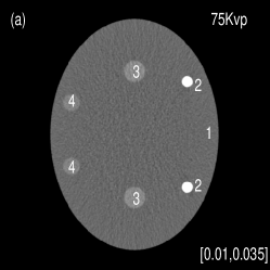
Figure 1: CT images of the digital phantom: (a) The low-energy: 75 kVp and (b) The high-energy: 140 kVp. Display window is $[0.01,0.035]\mathrm{mm}^{-1}$. The components of ROIs are bone (ROI1), muscle (ROI2), mixture (ROI3), fat (ROI4) and air (ROI5).

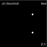
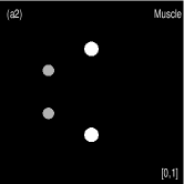
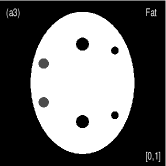
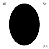
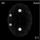
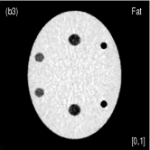
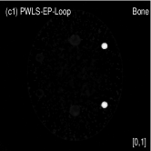
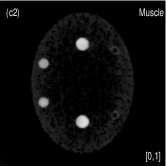
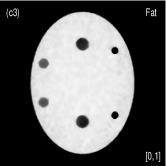
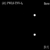
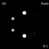
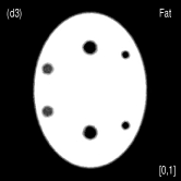
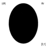
Figure 2: Material images of ground truth (the $1^{st}$ row), Direct Inversion (the $2^{nd}$ row), PWLS-DP-LOOP (the $3^{rd}$ row) and PWLS-TNV-$\ell_{0}$ (the $4^{th}$ row). The display windows are shown in the bottom-right corners.

We implemented the direct inversion MMD method in mendonca2014a and used its results as the initialization for the PWLS-EP-LOOP method xue2017statistical and the PWLS-TNV-$\ell_{0}$ method respectively. Fig. 2 (a) shows the true material images. Fig. 2 (b), (c) and (d) show the decomposed basis material images by the Direct inversion, the PWLS-EP-LOOP and the PWLS-TNV-$\ell_{0}$ method respectively. The PWLS-TNV-$\ell_{0}$ method reduced noise and crosstalk in the component images, especially for the muscle image, compared to the PWLS-EP-LOOP method. To quantitatively analyze performances of different methods, we calculated evaluation metrics of decomposed basis material images in several ROIs located within uniform areas shown with dashed line circles in Fig. 1 (b). Table 1 summarizes the means and noise STDs of the decomposed basis material images. For the Direct Inversion, the PWLS-EP-LOOP and the proposed PWLS-TNV-$\ell_{0}$ method, the volume fraction accuracies were $93.61\%$, $93.27\%$, and $99.31\%$ respectively. Compared with Direct Inversion and PWLS-EP-LOOP, the proposed method improved volume fraction accuracy by $5.7\%$ and $6.04\%$ respectively.

Table 1: The means and STDs of decomposed images within ROIs of the digital phantom.

Methods	ROI1	ROI2	ROI3		ROI4	ROI5
	Bone	Muscle	Muscle	Fat	Fat	Air
Ground Truth	$1\pm 0$	$1\pm 0$	$0.7\pm 0$	$0.3\pm 0$	$1\pm 0$	$1\pm 0$
Direct Inversion	$0.9964\pm 0.0073$	$0.7834\pm 0.1420$	$0.6753\pm 0.0749$	$0.3101\pm 0.0388$	$0.9087\pm 0.0384$	$0.9970\pm 0.0041$
PWLS-EP-LOOP	$0.9588\pm 0.0181$	$0.8107\pm 0.0221$	$0.6756\pm 0.0186$	$0.3187\pm 0.0121$	$0.9261\pm 0.0096$	$0.9976\pm 0.0038$
PWLS-TNV-$\ell_{0}$	$0.9989\pm 0.0143$	$0.9995\pm 0.0156$	$0.7071\pm 0.0353$	$0.2919\pm 0.0345$	$0.9983\pm 0.0020$	$0.9993\pm 0.0011$

III.3 Catphan©600 phantom study

We acquired the Catphan©600 phantom data on a tabletop cone-beam CT (CBCT) system whose geometry matched that of a Varian On-Board Imager (OBI) on the Trilogy radiation therapy machine. We inserted iodine solutions with nominal concentrations of $10~{}\mathrm{mg}/\mathrm{ml}$ and $5~{}\mathrm{mg}/\mathrm{ml}$ into the phantom. There were $1024\times 768$ pixels with a physical size of $0.388~{}\mathrm{mm}\times 0.388~{}\mathrm{mm}$ per pixel on the CB4030 flat-panel detector (Varian Medical Systems). The DECT measurements were obtained at $75$ kVp and $125$ kVp with a tube current of $80$ mA and a pulse width of $13$ ms. We acquired $655$ projections over $[0^{\circ},360^{\circ})$ in each scan. Using a fan-beam geometry with a longitudinal beam width of $15~{}\mathrm{mm}$ on the detector niu2010shading , We acquired projections with scatter contamination inherently suppressed. We used a contrast rod slice of the Catphan©600 phantom to evaluated the proposed method. We reconstructed attenuation images of size $512\times 512$ with a pixel size of $0.5\mathrm{mm}\times 0.5~{}\mathrm{mm}$. Fig. 3 shows the low- and high-energy CT images. Fig. 3(a) identifies the rods with labels: Teflon (labeled as $\#1$), Delrin (labeled as $\#2$), Iodine solution of $10~{}\mathrm{mg}/\mathrm{ml}$ (labeled as $\#3$), Polystyrene (labeled as $\#4$), low-density Polyethylene (LDPE) (labeled as $\#5$), Polymethylpentene (PMP) (labeled as $\#6$), Iodine solution of $5~{}\mathrm{mg}/\mathrm{ml}$ (labeled as $\#7$). Fig. 3(b) shows selected basis materials and ROIs in white dashed line circles: Teflon (ROI1), Delrin (ROI2), Iodine solution of $10~{}\mathrm{mg}/\mathrm{ml}$ (ROI3), PMP (ROI4), Inner soft tissue (ROI5) and Air (ROI6).

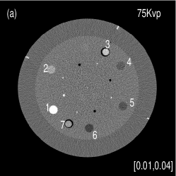
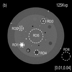
Figure 3: CT images of the Catphan©600 phantom on the contrast rods slice: (a) The low-energy: 75 kVp and (b) The high-energy: 125 kVp. Display window is $[0.01,0.04]\mathrm{mm}^{-1}$. The components of ROIs are Teflon (ROI1), Delrin (ROI2), Iodine of $10~{}\mathrm{mg}/\mathrm{ml}$ (ROI3), PMP (ROI4), Inner soft tissue (ROI5) and Air (ROI6).

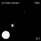
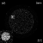
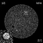
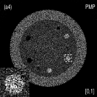
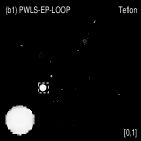
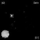
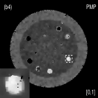
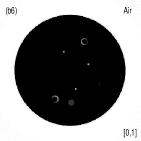
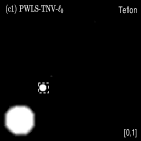
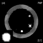
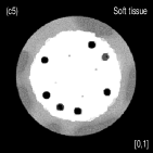
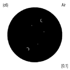
Figure 4: Material images of Direct Inversion (the $1^{st}$ row), PWLS-DP-LOOP (the $2^{rd}$ row) and PWLS-TNV-$\ell_{0}$ (the $3^{nd}$ row). The decomposed Teflon (the $1^{st}$ column), delrin (the $2^{ed}$ column), iodine solution(the $3^{nd}$ column), PMP (the $4^{th}$ column), soft tissue (the $5^{th}$ column) and air (the $6^{th}$ column) images of the Catphan©600 phantom on the contrast rods slice . The display windows are shown in the bottom-right corners.

Fig. 4 shows the decomposed material images by the Direct Inversion, the PWLS-EP-LOOP and the PWLS-TNV-$\ell_{0}$ method. The left corners of the $1^{st}$ to the $4^{th}$ column of Fig. 4 show enlarged rods that are highlighted with white dashed boxes in decomposed material images. Table 2 summarizes the means and noise STDs of ROIs of decomposed basis material images. The volume fraction (VF) accuracies were $68.62\%$, $79.33\%$, and $99.88\%$ for the Direction Inversion, the PWLS-EP-LOOP and the PWLS-TNV-$\ell_{0}$ method, respectively. Compared with the Direct Inversion and the PWLS-EP-LOOP method, the proposed PWLS-TNV-$\ell_{0}$ method increases the VF accuracy by $31.18\%$ and $20.45\%$ respectively.

Table 2: The means and STDs of decomposed images within each ROI of Catphan©600.

Methods	ROI1	ROI2	ROI3	ROI4	ROI5	ROI6
	Teflon	Delrin	Iodine	PMP	Soft Tissue	Air
Ground Truth	$1\pm 0$	$1\pm 0$	$1\pm 0$	$1\pm 0$	$1\pm 0$	$1\pm 0$
Direct Inversion	$0.9578\pm 0.0642$	$0.5852\pm 0.3340$	$0.6190\pm 0.3290$	$0.5067\pm 0.3088$	$0.4265\pm 0.3309$	$0.9995\pm 0.0037$
PWLS-EP-LOOP	$0.9615\pm 0.0043$	$0.7306\pm 0.0367$	$0.7112\pm 0.0188$	$0.7788\pm 0.0071$	$0.5779\pm 0.0277$	$0.9999\pm 0.0018$
PWLS-TNV-$\ell_{0}$	$1.0000\pm 0.0025$	$0.9971\pm 0.0037$	$1.0026\pm 0.0074$	$0.9989\pm 0.0093$	$1.0002\pm 0.0001$	$1.0001\pm 0.0001$

Table 3 summarizes the average electron densities of contrast rods and RMSE($\%$) of electron density for the three MMD methods. The RMSE($\%$) was $12.27\%$, $11.81\%$ and $4.42\%$ for the Direct Inversion method, the PWLS-EP-LOOP method and the proposed PWLS-TNV-$\ell_{0}$ method, respectively. The proposed PWLS-TNV-$\ell_{0}$ method suppressed noise, decreases crosstalk and increased decomposition accuracy in the material images, while maintaining high image quality.

Table 3: Electron densities inside the Catphan©600 contrast rods. The numbers of the rods are marked in Fig. 3(a). The last column is RMSE$(\%)$ of the seven rods. The electron density of iodine solutions is calculated based on iodine concentrations. The unit of the electron density is $10^{23}\mathrm{e}/\mathrm{cm}^{3}.$

Rods	1	2	3	4	5	6	7
	Teflon	Delrin	Iodine(10 mg/ml)	Polystyrene	LDPE	PMP	Iodine(5 mg/ml)	RMSE$(\%)$
Ground truth	$6.240$	$4.525$	$3.368$	$3.400$	$3.155$	$2.851$	$3.356$
Direct Inversion	$6.158$	$4.127$	$3.882$	$2.984$	$2.729$	$2.274$	$3.370$
Average Percentage Errors E$(\%)$	$1.32\%$	$8.80\%$	$15.25\%$	$12.24\%$	$13.49\%$	$20.23\%$	$0.42\%$	$12.27\%$
PWLS-EP-LOOP	$6.171$	$4.288$	$3.936$	$3.140$	$2.769$	$2.243$	$3.348$
Average Percentage Errors E$(\%)$	$1.10\%$	$5.23\%$	$16.85\%$	$7.65\%$	$12.23\%$	$21.32\%$	$0.25\%$	$11.81\%$
PWLS-TNV-$\ell_{0}$	$6.242$	$4.525$	$3.390$	$3.173$	$2.854$	$2.854$	$3.375$
Average Percentage Errors E$(\%)$	$0.02\%$	$0.00\%$	$0.66\%$	$6.68\%$	$9.54\%$	$0.11\%$	$0.56\%$	$4.42\%$

III.4 Pelvis Data Study

Table 4: Data acquisition parameters applied in pelvis data acquisition.

Siemens SOMATOM Definition flash CT	Peak voltage (kVp)	X-ray Tube Current (mA)	Exposure Time(s)	Current-exposure Time Product (mAs)	Noise STD ($\mathrm{mm}^{-1}$)	Helical Pitch	Gantry Rotation Speed (circle/second)
High-energy CT image	$140$	$146$	$0.500$	$73.0$	$4.09\mathrm{e}-04$	$0.7$	$0.28$
Low-energy CT image	$100$	$186$	$0.500$	$93.0$	$7.27\mathrm{e}-04$	$0.7$	$0.28$

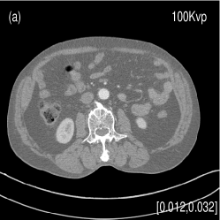
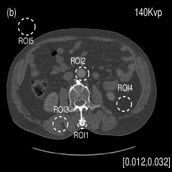
Figure 5: CT images of a pelvis patient. (a) The low-energy: 100 kVp and (b) The high-energy: 140 kVp. Display window is [0.012, 0.032] $\mathrm{mm}^{-1}$. The major components of ROIs are bone (ROI1), iodine solution (ROI2), muscle (ROI3), fat (ROI4) and air (ROI5).

We also evaluated the proposed PWLS-TNV-$\ell_{0}$ method using clinical pelvis data. The patient’s pelvis data was acquired by Siemens SOMATOM Definition flash CT scanner using DECT imaging protocol. Table 4 lists acquisition parameters in the pelvis data scan. Fig. 5 shows the high- and low-energy CT images of the pelvis data. Fig.5 (b) shows selected basis materials, bone, iodine, muscle, fat and air, and their assosicated ROIs highlightened in white dashed line circles. We implemented the Direct Inversion method in mendonca2014a and used its results as the initialization for the PWLS-EP-LOOP xue2017statistical and the proposed PWLS-TNV-$\ell_{0}$ method. Fig. 6 shows the decomposed material images by the Direct Inversion, the PWLS-EP-LOOP and the PWLS-TNV-$\ell_{0}$ method. Table 5 summarizes the means and noise STDs of the decomposed material images by the above three methods. The volume fraction (VF) accuracies are $80.48\%$, $86.50\%$, and $99.96\%$ for the Direct Inversion method, the PWLS-EP-LOOP method and the proposed PWLS-TNV-$\ell_{0}$, respectively. Compared with the Direct Inversion and PWLS-EP-LOOP method, the proposed method improves the VF accuracy by $19.48\%$ and $13.46\%$ respectively. The proposed PWLS-TNV-$\ell_{0}$ method decomposes basis material images more accurately, suppresses noise and decreases crosstalk, while retaining spatial resolution of the decomposed images compared to the other two methods.

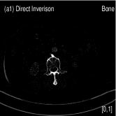
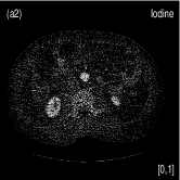
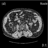
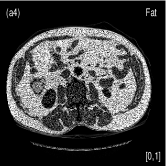
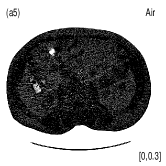
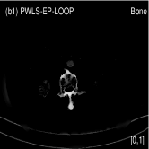
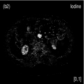
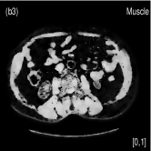
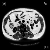
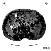
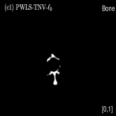
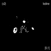
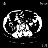
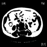
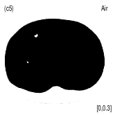
Figure 6: Material images of Direct Inversion (the $1^{st}$ row), PWLS-EP-LOOP (the $2^{rd}$ row) and PWLS-TNV-$\ell_{0}$ (the $3^{nd}$ row). The decomposed bone (the $1^{st}$ column), iodine (the $2^{ed}$ column), muscle (the $3^{nd}$ column), fat (the $4^{th}$ column) and air (the $5^{th}$ column) images. The display windows are shown in the bottom-right corners.

Table 5: The means and STDs of decomposed images within each ROI of pelvis data.

Methods	ROI1	ROI2	ROI3	ROI4	ROI5
	Bone	Iodine	Muscle	Fat	Air
Direct Inversion	$1.000\pm 0.000$	$0.6380\pm 0.2692$	$0.6623\pm 0.2603$	$0.7237\pm 0.2711$	$1.0000\pm 0.0000$
PWLS-EP-LOOP	$0.8868\pm 0.0055$	$0.7844\pm 0.1595$	$0.7914\pm 0.0194$	$0.8623\pm 0.0208$	$1.0000\pm 0.0000$
PWLS-TNV-$\ell_{0}$	$1.0012\pm 0.0129$	$0.9998\pm 0.0121$	$1.0003\pm 0.0084$	$1.0002\pm 0.0099$	$1.0000\pm 0.0003$

IV Discussion

We proposed a statistical image-domain MMD method for DECT, named PWLS-TNV-$\ell_{0}$. Its cost function is in the form of PWLS estimation with a negative log-likelihood term and three regularization terms. The first TNV regularization term considers structural correlation among basis material images, i.e., different material images share common or complementary edges and material images are piecewise constant. The second regularization term encourages sparsity of material types in each pixel, which is different from previous work mendonca2014a ; long2014multi-material that imposes a constraint that each pixel contains at most three materials. Considering volume and mass conservation, the third regularization term includes sum-to-one and box constraint which are imposed in the optimization process in previous work mendonca2014a ; long2014multi-material ; xue2017statistical . We applied the popular algorithm, ADMM, to optimizate the proposed PWLS-TNV-$\ell_{0}$ problem. Initialization is important for the PWLS-TNV-$\ell_{0}$ method since its cost function is non-convex. We set results of the Direct Inversion method mendonca2014a as initialization for the proposed PWLS-TNV-$\ell_{0}$ method to help with converging to a decent local minimum.

The PWLS-TNV-$\ell_{0}$ method requires to tune two regularization parameters and several other parameters when optimizing its cost function using ADMM. The choice of parameters significantly influences the decomposed material images. We need to determine appropriate combination of parameters for each DECT dataset. With the appropriate combination of parameters, the propose PWLS-TNV-$\ell_{0}$ method decreases noise while maintaining resolution of decomposed material images. How to choose the parameters is still a challenge problem and future work will investigate how to chose these parameters. The most time consuming operation in the proposed method is solving problem (36) which requires SVD operation for every pixel in each iteration. We will investigate acceleration methods to speed up the SVD operation in future work. Similar to our previous work xue2017statistical ; niu2014iterative , the statistical weight of the proposed PWLS-TNV-$\ell_{0}$ method was estimated by the calculated numerical variance of two manually selected homogeneous regions with a single material in both the high- and low-energy CT image. This variance estimation method assumes that the noise in the high- and low-energy CT images are uncorrelated, noise in pixels are uncorrelated and every pixel has the same noise variance. More accurate pixel-wise noise variance can be estimated on a serial of DECT images acquired from repeated scans on the same object. This method is not practical to implement on clinical patients due to accumulated high radiation dose. Zhang-O’Connor and Fessler proposed a fast method to predict variance images of PWLS or PL reconstructions with quadratic regularization from sinograms or pre-log data zhang2007fast . Li et al. proposed a computationally efficient technique for local noise estimation directly from CT images li2014adaptive . We will investigate noise covariance estimation methods and apply them to the PWLS-TNV-$\ell_{0}$ method in future work.

V Conclusion

We proposed an image-domain MMD method using DECT measurements and named it the PWLS-TNV-$\ell_{0}$ method. We imposed low rank property of material image gradients, sparsity of material composition and mass and volume conservation to help the proposed PWLS-TNV-$\ell_{0}$ method with estimating multiple material images from DECT measurements. To minimize the proposed cost function, we introduced auxiliary variables so that the original optimization problem can be divided into solvable subproblems by the ADMM method. Testing on simulated digital phantom, Catphan©600 phantom and clinical data, we concluded that the proposed PWLS-TNV-$\ell_{0}$ method suppresses noise and crosstalk, increases decomposition accuracy and maintains image resolution in the decomposed material images, compared to existing image-domain MMD methods using DECT measurements, the Direct Inversion and the PWLS-EP-LOOP method.

Appendix

The operators $\mathcal{D}$, $\mathcal{H}$, $\mathcal{P}$ corresponding with the subproblem of auxiliary variables, $u$,$v$ and $w$, are (39), (40), (41). We will give the calculative methods in details.

• The singular value thresholding operator, $\mathcal{D}_{\cdot}(\cdot)$, is the proximal operator associated with the nuclear norm cai2010singular . For $\tau\geq 0$ and $\bm{Y}\in\mathbb{R}^{n_{1}\times n_{2}}$, the singular value shrinkage operator obeys

  $$\mathcal{D}_{\tau}(\bm{Y})= \mathrm{prox}_{\lambda\|\cdot\|_{\ast}}(Y)$$

  $$= \arg\min_{\bm{X}}\tau\|\bm{X}\|_{\ast}+\frac{1}{2}\|\bm{X}-\bm{Y}\|_{F}^{2}.$$ (48)

  The singular value decomposition (SVD) of $\bm{Y}$ is

  $$\bm{Y}=\bm{U}\bm{\Sigma}\bm{V}^{\ast},$$ (49)

  where $\bm{U}\in\mathbb{R}^{n_{1}\times r}$, $\bm{V}\in\mathbb{R}^{n_{2}\times r}$ with orthonormal columns, and $\bm{\Sigma}=\rm{diag}(\{\sigma_{i}\}_{1\leq i\leq r})$. We obtain

  $$\mathcal{D}_{\tau}(\bm{Y}):=\bm{U}\mathcal{D}_{\tau}(\bm{\Sigma})\bm{V}^{\ast},$$ (50)

  where $\mathcal{D}_{\tau}(\bm{\Sigma})=\rm{diag}(\{\sigma_{i}-\tau\}_{+})$, $\{t\}_{+}=\max(0,t)$.

  For each pixel $j$, we have

  $$\bm{u}^{n+1}(:,:,j) =\mathcal{D}_{\frac{\beta_{1}}{\gamma_{1}}}([\bm{D}\bm{x}^{n+1}+\frac{\bm{p}^{n}_{1}}{\gamma_{1}}](:,:,j)),$$

  $$j= 1,\cdots,N_{p}.$$ (51)

• For nonnegative $\lambda$ and vector $x$, the hard thresholding operator blumensath2008iterative ; Trzasko2007Sparse is defined as

  $$\mathcal{H}_{\lambda}(x)=\mathrm{prox}_{\lambda\|\cdot\|_{0}}(x)=\arg\min_{y}\lambda\|y\|_{0}+\frac{1}{2}\|y-x\|_{2}^{2},$$ (52)

  with

  $$(\mathcal{H}_{\lambda}(x))_{i}=\left\{\begin{array}[]{lll}x_{i}&\textrm{if $|x_{i}|>\sqrt{2\lambda}$},\\ \{0,x_{i}\}&\textrm{if $|x_{i}|=\sqrt{2\lambda}$},\\ 0&\textrm{if $|x_{i}|<\sqrt{2\lambda}$}.\end{array}\right.$$ (53)

  The closed-form solution for (37) is obtained by

  $$\bm{v}^{n+1}=\mathcal{H}_{\frac{\beta_{2}}{\gamma_{2}}}(\nabla\bm{x}^{n+1}+\frac{\bm{p}^{n}_{2}}{\gamma_{2}}).$$ (54)

• For nonnegative $\lambda$ and vector $x$, we define

  $$\mathcal{P}_{\lambda^{+}}(x)=\mathrm{prox}_{\chi_{S}(\cdot)}(x)=\arg\min_{y}\chi_{S}(y)+\frac{1}{2}\|y-x\|_{2}^{2},$$ (55)

  where $S=\{x:\sum_{i}x_{i}=\lambda,x_{i}\geq 0\}$. Specifically,

  $$(\mathcal{P}_{\lambda^{+}}(x))_{i}=\{x_{i}-\hat{t}\}_{+}$$ (56)

  where  $\hat{t}:=\frac{1}{n-k}(\sum_{j=k+1}^{n}x_{(j)}-\lambda)$  with  $k:=\max\{p:x_{(p+1)}\geq\frac{1}{n-p}(\sum_{j=p+1}^{n}x_{(j)}-\lambda)\}$ and $x_{(1)}\leq\cdots\leq x_{(n)}$ is the permutation of $x$ in ascending order kyrillidis2012sparse ; chen2011projection .

  For each pixel $j$, subproblem (38) is the projection on to a simplex,

  $$(\bm{w}^{n+1})_{j} =\mathcal{P}_{1^{+}}((\bm{x}^{n+1}+\frac{\bm{p}^{n}_{3}}{\gamma_{3}})_{j}),$$

  $$j =1,\cdots N_{p}.$$ (57)

References

- (1) Robert E Alvarez and Albert Macovski. Energy-selective reconstructions in X-ray computerised tomography. Physics in medicine and biology, 21(5):733, 1976.
- (2) Robert E Alvarez and Albert Macovski. X-ray spectral decomposition imaging system, 1977.
- (3) Thomas Blumensath and Mike E Davies. Iterative thresholding for sparse approximation. Journal of Fourier Analysis and Applications, 14(5):629–654, 2008.
- (4) Hans Bornefalk and Mats Danielsson. Photon-counting spectral computed tomography using silicon strip detectors: a feasibility study. Physics in medicine and biology, 55(7):1999, 2010.
- (5) Jianfeng Cai, Emmanuel J Candès, and Zuowei Shen. A singular value thresholding algorithm for matrix completion. SIAM Journal on Optimization, 20(4):1956–1982, 2010.
- (6) Yunmei Chen and Xiaojing Ye. Projection onto a simplex. arXiv preprint arXiv:1101.6081, 2011.
- (7) Huanjun Ding, Hao Gao, Bo Zhao, Hyo-Min Cho, and Sabee Molloi. A high-resolution photon-counting breast CT system with tensor-framelet based iterative image reconstruction for radiation dose reduction. Physics in medicine and biology, 59(20):6005, 2014.
- (8) Hao Gao, Hengyong Yu, Stanley Osher, and Ge Wang. Multi-energy CT based on a prior rank, intensity and sparsity model (PRISM). Inverse problems, 27(11):115012, 2011.
- (9) Thomas A Goldstein and Stanley Osher. The Split Bregman Method for L1-regularized Problems. SIAM Journal on Imaging Sciences, 2(2):323–343, 2009.
- (10) PV Granton, SI Pollmann, NL Ford, M Drangova, and DW Holdsworth. Implementation of dual-and triple-energy cone-beam micro-ct for postreconstruction material decomposition. Medical physics, 35(11):5030–5042, 2008.
- (11) Avinash C Kak and Malcolm Slaney. Principles of computerized tomographic imaging. SIAM, 2001.
- (12) Anastasios Kyrillidis, Stephen Becker, Volkan Cevher And, and Christoph Koch. Sparse projections onto the simplex. 28(2):280–288, 2012.
- (13) Aurelie D Laidevant, Serghei Malkov, Chris I Flowers, Karla Kerlikowske, and John A Shepherd. Compositional breast imaging using a dual-energy mammography protocol. Medical physics, 37(1):164–174, 2010.
- (14) Peter Lamb, Dushyant V Sahani, Jorge M Fuentes-Orrego, Manuel Patino, Asish Ghosh, and Paulo RS Mendonça. tratification of patients with liver fibrosis using dual-energy CT. IEEE transactions on medical imaging, 34(3):807–815, 2015.
- (15) Liang Li, Zhiqiang Chen, Wenxiang Cong, and Ge Wang. Spectral CT modeling and reconstruction with hybrid detectors in dynamic-threshold-based counting and integrating modes. IEEE transactions on medical imaging, 34(3):716–728, 2015.
- (16) Zhoubo Li, Lifeng Yu, Joshua D Trzasko, David S Lake, Daniel J Blezek, Joel G Fletcher, Cynthia H McCollough, and Armando Manduca. Adaptive nonlocal means filtering based on local noise level for CT denoising. Medical physics, 41(1), 2014.
- (17) Jiulong Liu, Huanjun Ding, Sabee Molloi, Xiaoqun Zhang, and Hao Gao. TICMR: Total image constrained material reconstruction via nonlocal total variation regularization for spectral CT. IEEE transactions on medical imaging, 35(12):2578–2586, 2016.
- (18) Xin Liu, Lifeng Yu, Andrew N Primak, and Cynthia H McCollough. Quantitative imaging of element composition and mass fraction using dual-energy CT: Three-material decomposition. Medical physics, 36(5):1602–1609, 2009.
- (19) Yong Long and Jeffrey A Fessler. Multi-Material Decomposition Using Statistical Image Reconstruction for Spectral CT. IEEE Transactions on Medical Imaging, 33(8):1614–1626, 2014.
- (20) A Macovski, RE Alvarez, JL-H Chan, JP Stonestrom, and LM Zatz. Energy dependent reconstruction in X-ray computerized tomography. Computers in biology and medicine, 6(4):325IN7335–334336, 1976.
- (21) William H Marshall Jr, Robert E Alvarez, and Albert Macovski. Initial results with prereconstruction dual-energy computed tomography (predect). Radiology, 140(2):421–430, 1981.
- (22) Paulo R S Mendonca, Peter Lamb, and Dushyant V Sahani. A Flexible Method for Multi-Material Decomposition of Dual-Energy CT Images. IEEE Transactions on Medical Imaging, 33(1):99–116, 2014.
- (23) Paulo RS Mendonça, Rahul Bhotika, Mahnaz Maddah, Brian Thomsen, Sandeep Dutta, Paul E Licato, and Mukta C Joshi. Multi-material decomposition of spectral CT images. In SPIE Medical Imaging, pages 76221W–76221W. International Society for Optics and Photonics, 2010.
- (24) Paulo RS Mendonca, Peter Lamb, and Dushyant V Sahani. A flexible method for multi-material decomposition of dual-energy CT images. IEEE transactions on medical imaging, 33(1):99–116, 2014.
- (25) Frank Natterer. The mathematics of computerized tomography. SIAM, 2001.
- (26) Tianye Niu, Xue Dong, Michael Petrongolo, and Lei Zhu. Iterative image-domain decomposition for dual-energy CT. Medical physics, 41(4), 2014.
- (27) Tianye Niu, Mingshan Sun, Josh Star-Lack, Hewei Gao, Qiyong Fan, and Lei Zhu. Shading correction for on-board cone-beam CT in radiation therapy using planning MDCT images. Medical physics, 37(10):5395–5406, 2010.
- (28) NIST,X-Ray Mass Attenuation Coefficients.(https://www.nist.gov/pml/x-ray-mass-attenuation-coefficients).
- (29) Siemens.(https://bps-healthcare.siemens.com/cv_oem/radIn.asp).
- (30) David S Rigie and Patrick J La Rivière. Joint reconstruction of multi-channel, spectral CT data via constrained total nuclear variation minimization. Physics in medicine and biology, 60(5):1741, 2015.
- (31) David S Rigie and Patrick J La Rivière. A generalized vectorial total-variation for spectral CT reconstruction. In Proc.3rd Intl.Mtg.on image formation in X-ray CT.
- (32) Polad M Shikhaliev and Shannon G Fritz. Photon counting spectral CT versus conventional CT: comparative evaluation for breast imaging application. Physics in medicine and biology, 56(7):1905, 2011.
- (33) J Peter Stonestrom, Robert E Alvarez, and Albert Macovski. A framework for spectral artifact corrections in X-ray CT. IEEE Transactions on Biomedical Engineering, (2):128–141, 1981.
- (34) Timothy P Szczykutowicz and Guang-Hong Chen. Dual energy ct using slow kvp switching acquisition and prior image constrained compressed sensing. Physics in medicine and biology, 55(21):6411, 2010.
- (35) Joshua D Trzasko, Armando Manduca, and Eric Borisch. Sparse MRI reconstruction via multiscale l0-continuation. IEEE/SP 14th Workshop on Statistical Signal Processing, page 176 C180, 2007.
- (36) Yi Xue, Ruoshui Ruan, Xiuhua Hu, Yu Kuang, Jing Wang, Yong Long, and Tianye Niu. Statistical image-domain multi-material decomposition for dual-energy CT. Medical Physics, 2017.
- (37) Yingying Zhang-O’Connor and Jeffrey A Fessler. Fast predictions of variance images for fan-beam transmission tomography with quadratic regularization. IEEE transactions on medical imaging, 26(3):335–346, 2007.