X-ray Measurements of the Particle Acceleration Properties at Inward Shocks in Cassiopeia A

Abstract

We present new evidence that the bright non-thermal X-ray emission features in the interior of the Cassiopeia A supernova remnant (SNR) are caused by inward moving shocks based on Chandra and NuSTAR observations. Several bright inward-moving filaments were identified using monitoring data taken by Chandra in 2000–2014. These inward-moving shock locations are nearly coincident with hard X-ray (15–40 keV) hot spots seen by NuSTAR. From proper motion measurements, the transverse velocities were estimated to be in the range $\sim$2,100–3,800 km s^-1 for a distance of 3.4 kpc. The shock velocities in the frame of the expanding ejecta reach values of $\sim$5,100–8,700 km s^-1, slightly higher than the typical speed of the forward shock. Additionally, we find flux variations (both increasing and decreasing) on timescales of a few years in some of the inward-moving shock filaments. The rapid variability timescales are consistent with an amplified magnetic field of $B\sim$ 0.5–1 mG. The high speed and low photon cut-off energy of the inward-moving shocks are shown to imply a particle diffusion coefficient that departs from the Bohm regime ($k_{0}=D_{0}/D_{\rm 0,Bohm}\sim$ 3–8) for the few simple physical configurations we consider in this study. The maximum electron energy at these shocks is estimated to be $\sim$8–11 TeV, smaller than the values of $\sim$15–34 TeV inferred for the forward shock. Cassiopeia A is dynamically too young for its reverse shock to appear to be moving inward in the observer frame. We propose instead that the inward-moving shocks are a consequence of the forward shock encountering a density jump of $\gtrsim$ 5–8 in the surrounding material.

1 Introduction

Shock waves in young supernova remnants (SNRs) are excellent astrophysical laboratories for understanding the process of particle acceleration. An important observational advance was the imaging of synchrotron X-ray–emitting rims in SN1006 (Koyama et al., 1995) which strengthened arguments for the shock acceleration of electrons to TeV energies in the forward shocks of young SNRs. More recently, GeV and TeV $\gamma$-ray spectral observations have been shown to be well described by the decay of pions produced by energetic protons interacting with ambient gas (e.g., Ackermann et al., 2013), providing strong evidence for proton acceleration in SNRs. From these studies as well as several others using a variety of different techniques, it is now widely accepted that electron and proton acceleration occurs in SNRs. Diffusive shock acceleration (DSA: Bell, 1978; Blandford & Eichler, 1987) in the forward shocks of remnants is the leading candidate for the process and can account for the majority of Galactic cosmic rays. On the other hand, observational evidence for particle acceleration at SNR reverse shocks, which propogate inward through the expanding ejecta, has not been clearly demonstrated, although there have been some theoretical studies (e.g., Ellison et al., 2005; Telezhinsky et al., 2012, 2013).

Cassiopeia A with an age of $\sim 350$ yr (Fesen et al., 2006) is one of the most well-studied young Galactic SNRs. Non-thermal X-ray emission has been detected from both the outer rim and interior positions (e.g., Hughes et al., 2000; Vink & Laming, 2003; Bamba et al., 2005; Helder & Vink, 2008; Maeda et al., 2009; Grefenstette et al., 2015). In particular, the brightest non-thermal X-ray emission comes from the western limb slightly interior to the forward shock position and is also strongly associated with TeV $\gamma$-ray emission (e.g., Aharonian et al., 2001; Albert et al., 2007; Maeda et al., 2009; Acciari et al., 2010; Grefenstette et al., 2015). Those features naturally suggest efficient production of accelerated particles in this region, however, the origin of the energetic electrons in the interior of the remnant remains a mystery.

Radio and X-ray observations of Cassiopeia A have found that some features are moving back toward the expansion center (Anderson & Rudnick, 1995; Keohane et al., 1996; DeLaney et al., 2004); we refer to these as “inward shocks”. The inward shocks are concentrated in the south and west between azimuths of 170^∘ to 300^∘. Helder & Vink (2008) have suggested that the bright non-thermal X-rays at the reverse shock region could be due to the locally higher reverse shock velocity($v_{s}\sim$ 6,000 km s^-1) of the inward moving shock filaments. It was recognized even earlier that such high reverse shock velocities or inward moving filaments required a more complex structure for the circumstellar medium in the west. For example, Keohane et al. (1996) argued for a physical connection with a local molecular cloud based on strong radio and X-ray absorbing structures seen near the inward moving shocks (see also Sanders, 2006; Hwang & Laming, 2012, for the X-ray absorbing structures). Recent millimeter observations have additionally suggested an interaction between the shock front and a nearby molecular cloud (Kilpatrick et al., 2014). Such a high density cloud would also be consistent with the pion-decay scenario for the $\gamma$-ray emission from Cassiopeia A. Finally, a shock-cloud interaction is considered to have a connection with the non-thermal X-rays (Sano et al., 2010, 2013, 2015; Inoue et al., 2012).

Although these various non-thermal features appear to be related, a unified picture for the western reverse shock region of Cassiopeia A has yet to be established. As a step in further understanding the particle acceleration properties in this exceptional region of the remnant, here we report new X-ray kinematic and intensity properties for bright inward moving filaments. Using long-term monitoring data from Chandra, we determine the proper motion and temporal flux variation for a set of six bright non-thermal filaments. We then combine this with results from hard X-ray measurements by NuSTAR to determine the physical properties (e.g., magnetic field, diffusion coefficient, maximum electron energy, and acceleration and cooling timescales) of the particle acceleratio process in these shocks.

2 Observation and Data Reduction

2.1 Chandra

The Chandra ACIS-S have observed Cassiopeia A several times since the launch in 1999 (e.g., Hwang et al., 2000, 2004; Patnaude et al., 2011; Hwang & Laming, 2012; Patnaude & Fesen, 2014). The data used in our analysis are listed in Table 1. We reprocessed the event files (from level 1 to level 2) to remove pixel randomization and to correct for CCD charge transfer efficiencies using CIAO (Fruscione et al., 2006) version 4.6 and CalDB 4.6.3. The bad grades were filtered out and good time intervals were reserved.

Table 1: Chandra observations.

ObsID.	date	exp.	angle	shift values
	YYYY/MM/DD	(ks)	(deg)	($\Delta x$, $\Delta y$)
114 .	2000/01/30	49.9	323.4	($-0.09$, $+0.34$)
1952 .	2002/02/06	49.6	323.4	($-0.36$, $+0.38$)
4634 .	2004/04/28	148.6	59.2	($+0.15$, $-0.20$)
4635 .	2004/05/01	135.0	59.2	($-0.05$, $-0.27$)
4636 .	2004/04/20	143.5	49.8	($-0.09$, $-0.21$)
4637 .	2004/04/22	163.5	49.8	($-0.04$, $-0.22$)
4638 .	2004/04/14	164.5	40.3	(reference)
4639 .	2004/04/25	79.0	49.8	($-0.04$, $-0.35$)
5196 .	2004/02/08	49.5	325.5	($+0.07$, $+0.03$)
5319 .	2004/04/18	42.3	49.8	($-0.08$, $+0.08$)
5320 .	2004/05/05	54.4	65.1	($+0.03$, $-0.41$)
9117 .	2007/12/05	24.8	278.1	($-0.01$, $+0.87$)
9773 .	2007/12/08	24.8	278.1	($-0.19$, $+0.89$)
10935 .	2009/11/02	23.3	239.7	($-0.53$, $+0.53$)
12020 .	2009/11/03	22.4	239.7	($-0.50$, $+0.32$)
10936 .	2010/10/31	32.2	236.5	($-0.44$, $-0.11$)
13177 .	2010/11/02	17.2	236.5	($+0.00$, $-0.02$)
14229 .	2012/05/15	49.1	75.4	($-0.52$, $-0.60$)
14480 .	2013/05/20	48.8	75.1	($-0.38$, $+0.63$)
14481 .	2014/05/12	48.4	75.1	($+0.08$, $+0.50$)

In order to align the images, we used the Central Compact Object (CCO) as a fiducial source. Because of lack of other certain fiducial sources around Cassiopeia A, we registered only the CCO for the alignment. First, we determined the CCO position using wavdetect implemented in CIAO. Next, shift values between two ObsIDs were computed with wcs_match script. By using these values, we finally updated the aspect solutions of the event files using wcs_update. We here used the ObsID 4638 as the reference of the alignment. The shift values are summarized in Table 1. In the following section 3.2, we assumed official systematic errors of $\sim$0.5^′′ for the positional accuracy although we aligned the images. Our image alignment using the CCO could reduce the uncertainties. However, there would still be other positional uncertainties (e.g., roll angle, proper motion of the CCO, etc.). For example, Fesen et al. (2006) have estimated a transverse velocity of $\simeq$350 km s^-1 for the CCO. This corresponds to a shift of $\sim$0.3^′′ ($<$ 1 pixel) for 14 years at the distance of 3.4 kpc (see Reed et al., 1995, for the distance), which is within the systematic errors.

Table 2: NuSTAR observations.

ObsID.	Date	Exp.
	YYYY/MM/DD	(ks)
40001019002	2012/08/18	294
40021001002	2012/08/27	190
40021001004	2012/10/07	29
40021001005	2012/10/07	228
40021002002	2012/11/27	288
40021002006	2013/03/02	160
40021002008	2013/03/05	226
40021002010	2013/03/09	16
40021003002	2013/05/28	13
40021003003	2013/05/28	216
40021011002	2013/10/30	246
40021012002	2013/11/27	239
40021015002	2013/12/21	86
40021015003	2013/11/23	160
Total		$\sim$2.4 Ms

2.2 NuSTAR

NuSTAR, which is composed of two co-aligned X-ray telescopes (FPMA and FPMB) observing the sky in the energy range 3–79 keV (Harrison et al., 2013), has observed Cassiopeia A with a total of $\sim$ 2.4 Ms of exposure time during the first two years after the launch in 2012 (see Table 2). The first hard X-ray imaging revealed ⁴⁴Ti distribution and morphology of $>$15 keV emission in Cassiopeia A for the first time (Grefenstette et al., 2014, 2015, 2017).

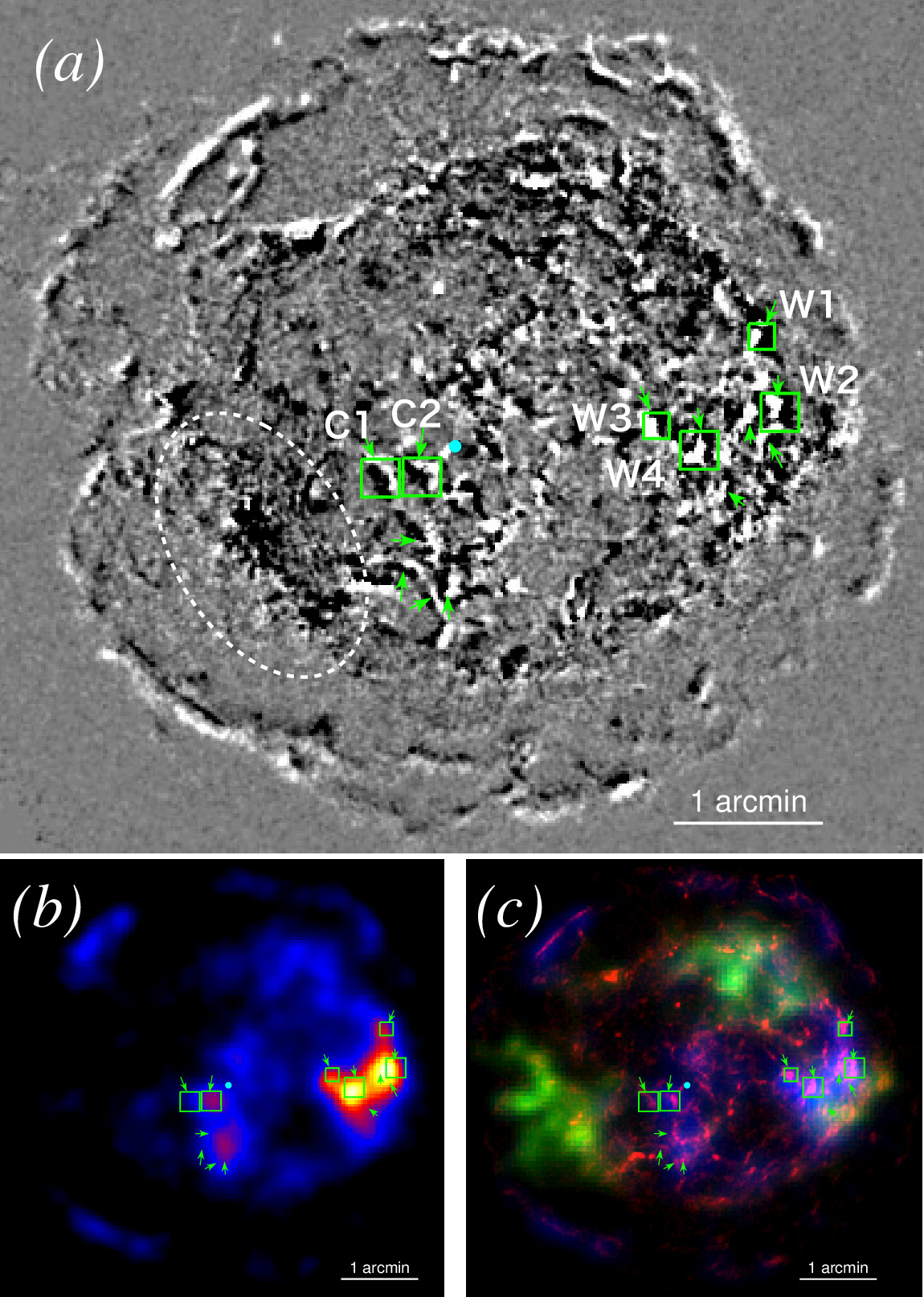
Figure 1: (a) Image difference in the 4.2–6 keV band of Cassiopeia A between 2000 and 2014 with Chandra. Adjacent black and white features show transverse motions of X-ray structures. Green arrows and boxes show the inward-shock positions defined by eye and the regions which were used for the proper-motion measurements. The boxes are identified by name (e.g., C1, W1) The box sizes are 21$\times$21 pixels (1 pixel = 0.492^′′) for W1 and W3, and 31$\times$31 pixels for C1, C2, W2 and W4, respectively. (b) The NuSTAR image in 15–40 keV band. The green arrows and boxes show the same as shown in the figure (a). (c) Three-color image of Cassiopeia A. Red, green and blue color show the 4.2–6 keV image with Chandra, the 6.54–6.92 keV image (around Fe-K emission) with Chandra and the 15–40 keV image with NuSTAR. The binning sizes for the 4.2–6 keV (Chandra), 6.54–6.92 keV (Chandra) and 15–40 keV (NuSTAR) images are 1$\times$1 pixels (0.492^′′$\times$0.492^′′), 8$\times$8 pixels (3.936^′′$\times$3.936^′′) and 1$\times$1 pixels (12.3^′′$\times$12.3^′′), respectively. The images were then smoothed with a Gaussian function with a sigma of 3 bins. The green arrows and boxes show the same as shown in the figure (a). Cyan dot shows the position of the central compact object (CCO).

Figure 2: Left side: X-ray images overlaid with proper-motion vectors obtained by the optical flow method, where the energy ranges are (a) a continuum band of 4.1-6.3 keV and (b) Si-K band of 1.7-2.1 keV. For the optical flow analysis, we used images taken in 2004 (ObsID. 5320) and 2014 (ObsID. 14481). The vector length is proportional to the actual shifting value. Blue and red show outward and inward motions, respectively. In these figures, small vectors whose proper motion is $\lesssim$ 0.05 arcsec yr^-1 are not shown. The field of view is 450$\times$450 pixels (= 3.69^′$\times$3.69^′). The center of the field of view, (x, y) = (225, 225) is the CCO location. The unit of the color bar is 10^-7 counts cm^-2 s^-1. Contours overlaid on the continuum and Si-K band images show 1, 5, 10, 15, 20$\times$10^-7 counts cm^-2 s^-1 and 3, 15, 30, 45, 60$\times$10^-7 counts cm^-2 s^-1, respectively. Right side: length of radial component of proper-motion vectors are shown in color maps in the continuum band (a^′) and the Si-K band (b^′). Positive and negative values correspond to outward and inward motions, respectively. The unit of the color scale is arcsec yr^-1. A proper motion of 0.15 arcsec yr^-1 corresponds to $\sim$2,400 km s^-1 at the distance of 3.4 kpc.

In order to compare the hard X-ray image (15–40 keV) with the Chandra image (4.2–6 keV), we analyzed all of the NuSTAR data. We reduced the data with the NuSTAR Data Analysis Software (NuSTARDAS) version 1.6.0 and NuSTAR calibration database (CALDB) version 20170503 to produce images and exposure maps for each telescope. All of the images were merged by using XIMAGE, taking into account the exposure maps (i.e., the unique time-dependent exposure and the vignetting function of the telescope) for each pointing. After the correction, we deconvoluved the merged image with the on-axis PSF image of the NuSTAR’s telescope. We used arestore script in CIAO for the deconvolution. Following the method in Grefenstette et al. (2015), we chose to halt the deconvolution after 50 iterations with a Richardson-Lucy method, and we obtained almost the same image as the published image (see Figure 1). For the NuSTAR imaging, the default aspect solution was used.

3 Analysis and Results

3.1 Soft and Hard X-ray imaging

In Figure 1(a), we show a difference image between 2000 and 2014 generated from Chandra data. Here we can see moving X-ray structures as previously reported (e.g., DeLaney et al., 2004; Patnaude & Fesen, 2009). All of the forward-shock filaments which are located at the outer rim are moving outward. On the other hand, there are several filaments near the center and toward the west that are moving inward (such filaments are identified with green arrows in the figure). Those filaments are the same inward-moving features (inward shocks) as reported in DeLaney et al. (2004). In particular, almost all the filaments toward the west seem to be inward shocks. By definition, the forward shock must always move to the outside of the remnant. Therefore, these inward shocks cannot be forward shocks seen projected on the interior of the remnant. In addition, part of the eastern region shows a uniform dark color (see a broken ellipse region in Figure 1). The eastern region is known to have a large contribution from thermal X-rays with a flux decline possibly due to adiabatic expansion (Sato et al., 2017). The dark eastern region in this figure is just another view of the prominent flux decay of the thermal emission.

In Figure 1(b), we show the 15–40 keV image with NuSTAR. As reported in previous studies (Willingale et al., 2002; Helder & Vink, 2008; Maeda et al., 2009; Grefenstette et al., 2015; Sato et al., 2017), most of the hard X-rays are located at the west and the center. Thus, we find a strong correlation between the inward-shock positions and the intensity peaks of the NuSTAR image.

In Figure 1(c), we compared the NuSTAR image with the soft X-ray images (4.2–6 keV: continuum emission & 6.54–6.92 keV: Fe-K emission) with Chandra. As reported in Sato et al. (2017), we can see a separation between the thermal X-ray distribution (Fe-K) and the hard X-ray distribution (which is spatially coincident with the inward-shock positions).

To clarify the motions of the shock filaments, we also compared images taken in 2004 (ObsID. 5320) and 2014 (ObsID. 14481) using a computer vision technique (optical flow). The dense optical flow algorithm we use is by Gunnar Farnebäck (Farnebäck, 2003) as implemented in OpenCV 3.2.0. This algorithm estimates displacement fields between two frames using quadratic polynomials to locally approximate the image flux. To reduce the noise, the estimate is made by averaging over local neighborhoods. Also, we here set statistical limits for the surface brightnesses. For the continuum and Si-K images, we ignore pixels whose surface brightness is $<$ 1$\times$10^-7 counts cm^-2 s^-1 and $<$ 3$\times$10^-7 counts cm^-2 s^-1 respectively, which corresponds to $\lesssim$ 1 counts with $\sim$ 50 ksec exposure time. Specifically, we used the calcOpticalFlowFarneback function with the following arguments: pyr_scale = 0.5, which specifies the image scale to build pyramids for each image, levels = 3, number of pyramid layers, winsize = 15, averaging window size, and poly_n = 5, size of the pixel neighborhood used for the polynomial approximation. As shown in Figure 2, we can visualize the motion of filaments (or small knots) as vector maps over the entire extent of the SNR. In the vector maps (Figure 2 (a) & (b)), we plot only large vectors whose proper motion is larger than $\sim$ 0.05 arcsec yr^-1 ($\approx$ 800 km s^-1 at the distance of 3.4 kpc), and we here found the large motions are strongly associated with filamentary (or knotty) structures. Also, we can see clearly that large motions are not identified at low count-rate regions.

In the continuum band (Figure 2 (a) & (a’)), the inward motions are concentrated in the interior. Indeed the positions of inward-moving features (blue spots in 2 (a’)) are very similar to the locations of the hard X-ray spots in Figure 1(b), providing further support for a connection between them. On the other hand, almost all of the small structures in the Si-K band are moving to the outside of the remnant (Figure 2 (b) & (b’)). These indicate a clear difference in the character of motion between the ejecta and the non-thermal emission components.

In this current study, we employ the optical flow method to provide a largely qualitative view of the expansion of the thermal ejecta and non-thermal shock filaments in Cassiopeia A. A detailed quantitative study of the results is beyond the scope of this initial investigation, although in future work, we will determine the accuracy and robustness of optical-flow proper-motion measurements for determining the global kinematics of young SNRs. In particular, combining comprehensive proper-motion and radial velocity measurements will further improve our understanding of the three-dimensional kinetics of young SNRs (e.g., DeLaney et al., 2010; Sato & Hughes, 2017a; Williams et al., 2017; Sato & Hughes, 2017b).

Table 3: Proper Motions and Spectral Parameters of the Inward-Shock Filaments in Cassiopeia A

	Imaging Analysis					Spectral Parameters in 2004
	center of the model frame	mean shift: $\Delta$x, $\Delta$y	proper motion	velocity	angle	Photon Index	flux in 4.2-6 keV
id	R.A., Decl. (epoch 2004)	(arcsec yr-1)	(arcsec yr-1)	(km s-1)	(degree)		(10-13 ergs cm-2 s-1)
west region
W1	23h23m12s.070, $+58^{\circ}$49′23′′.64	$-0.111\pm$0.026, $+0.077\pm$0.027	0.132$\pm$0.027	2130$\pm$440	145$\pm$11	2.11${}^{+0.05}_{-0.08}$	5.70$\pm$0.04
W2	23h23m11s.126, $+58^{\circ}$48′56′′.07	$-0.180\pm$0.026, $-0.089\pm$0.027	0.200$\pm$0.026	3210$\pm$420	206$\pm$8	2.00${}^{+0.03}_{-0.05}$	19.79$\pm$0.07
W3	23h23m17s.525, $+58^{\circ}$48′50′′.73	$-0.190\pm$0.027, $-0.113\pm$0.027	0.219$\pm$0.027	3540$\pm$440	211$\pm$7	2.18${}^{+0.05}_{-0.08}$	6.65${}^{+0.05}_{-0.03}$
W4	23h23m15s.310, $+58^{\circ}$48′40′′.87	$-0.126\pm$0.026, $-0.042\pm$0.027	0.129$\pm$0.026	2090$\pm$420	199$\pm$12	1.94${}^{+0.04}_{-0.07}$	10.04${}^{+0.06}_{-0.08}$
center region
C1	23h23m31s.829, $+58^{\circ}$48′29′′.70	$+0.215\pm$0.026, $-0.013\pm$0.027	0.213$\pm$0.027	3440$\pm$440	356$\pm$7	2.64${}^{+0.06}_{-0.09}$	6.56${}^{+0.08}_{-0.05}$
C2	23h23m29s.676, $+58^{\circ}$48′30′′.20	$+0.214\pm$0.027, $+0.101\pm$0.027	0.235$\pm$0.027	3800$\pm$440	25$\pm$6	2.24${}^{+0.05}_{-0.07}$	8.41${}^{+0.05}_{-0.07}$

3.2 Proper-Motion Measurements of the Inward-Shock Filaments

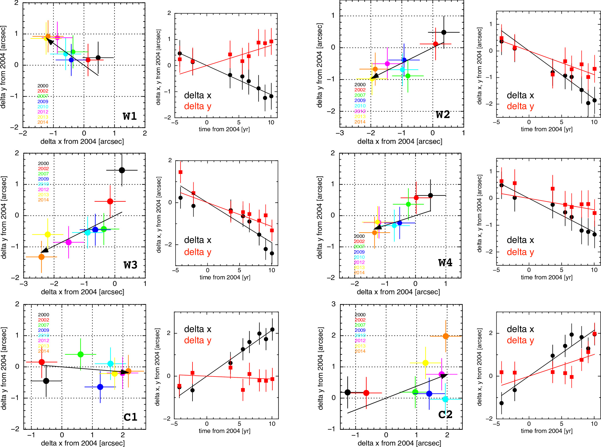
Figure 3: Results of the proper-motion measurements. Large panel shows a scatter plot of the best-fit positions (delta x vs. delta y). Here, each color identifies the best-fit positions from 2004. Black arrows show best-fit directions of the proper motions. Small panel that is placed close to the large one shows a plot of the best-fit positions as a function of time (delta x, y vs. time). Solid lines show the best-fit linear models for the estimations of the mean shift values summarized in Table 3. The error bars show 68 % confidence level, which include the systematic errors of ($\sigma_{\rm x}$, $\sigma_{\rm y}$) $=$ (0.5^′′, 0.5^′′). The fitting (statistical) errors are much smaller than the systematic uncertainties.

To measure proper motions of the inward-shock filaments, we extracted images from the box regions in Figure 1 and fitted with an image model. The fitting code used for this analysis was originally developed for proper-motion measurements for knots in Kepler’s SNR (Sato & Hughes, 2017b). Here, we used the 2004 image normalized by the image in each epoch as the model because the observation in 2004 has the longest exposure time that is about 20 times longer than that of the other observations (see Table 1). For obtaining the best-fit shifts, a maximum likelihood statistic for Poisson distributions was used (C-statistics; Cash, 1979), which minimizes

$$C=-2{\rm ln}~{}P=-2\Sigma_{i,j}(n_{i.j}~{}{\rm ln}~{}m_{i,j}-m_{i,j}-~{}{\rm ln}~{}n_{i.j}!)$$ (1)

where $n_{i,j}$ is the counts in pixel (i,j) of the image in each epoch, and $m_{i,j}$ is the model counts based on the 2004 image. The fitting errors can be estimated in the usual manner since the statistical distribution of $\Delta C=C-C_{\rm min}$ is similar to that of $\chi^{2}$ (Cash, 1979).

The fitting results are summarized in Figure 3 and Table 3. We found that the best-fit positions of those filaments are gradually shifting from the outside to the inside with large proper motion values: 0.129–0.219^′′ yr^-1 for the W filaments and 0.213–0.235^′′ yr^-1 for the C filaments. The best-fit x, y shifts and errors listed in Table 3 were determined by chi-square fitting with a linear function as shown in Figure 3. In the fitting, the slope provides the x, y shift (arcsec per year) with the error coming from $\Delta\chi^{2}$ = 1.0. Using the values, we determined the proper motions and errors (see Appendix for the method). For the assumed distance of 3.4 kpc (Reed et al., 1995) to the remnant, we estimate the filament velocities to be $\sim$2,100–3,800 km s^-1.

In the radio band, the kinematics of 304 knot structures over the entire remnant had been reported previously (Anderson & Rudnick, 1995). This work showed that the motions of many western knots deviated from that of knots in other regions and that some western knots were actually moving inward (see Fig. 5 and Fig. 6 in Anderson & Rudnick, 1995). In the X-ray band, continuum-dominated filaments with an inward motion were also found at azimuths between 170^∘ and 300^∘ (DeLaney et al., 2004). These features correspond to the inward shocks we found.

3.3 Flux Variations

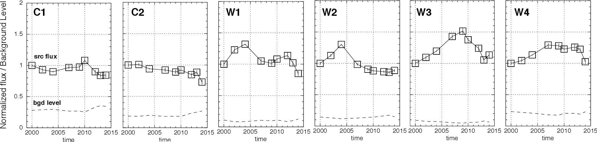
Figure 4: Time variations of the flux (black boxes) for each filament in the 4.2-6 keV band. The fluxes were normalized by the flux in the first epoch (2000). The error bars show 68 % confidence level ($\Delta\chi^{2}$ = 1.0). Broken lines show background levels in each epoch.

Here we investigate the X-ray light curves of the inward moving filaments. First we extracted spectra from each epoch for each inward-shock filament using the CIAO specextract command. For the source regions, we used ellipse regions which included the bright filament structures. These regions were shifted with time for taking the proper-motion effects into account. The background regions were selected from nearby low-brightness regions. The background-subtracted spectra were fitted in the 4.2–6 keV band using a power-law model in Xspec 12.9.0n (Arnaud, 1996).

We summarize the fitting results in Figure 4. For all of the western filaments, over the $\sim$14 yr span of observation X-ray fluxes increased by up to $\sim$40–50 % and afterward decreased to the initial flux level from epoch 2000. Background photons in the extracted spectrum are less than 30 % of the total, and fluctuate by $\lesssim\pm 20$ % (see black-broken lines in Figure 4). The change in the background rate from a uniform level could introduce a fluctuation in the filament’s X-ray flux of at most $\sim$9 %. Even given this effect, significant time variations of the X-ray flux are still present. Time intervals of the monitoring observations would mainly influence on the estimation accuracy of variable timescales. The intervals are $\sim$ 2 yrs from 2000 to 2007 and $\sim$ 1 yr from 2007 to 2014. Therefore, the uncertainty of estimated timescales would be $\pm$ 2 yr for the W1 and W2 filaments and $\pm$ 1 yr for the W3 and W4 filaments. Even taking these errors into consideration, the timescales are very short. For regions W1 and W2, the timescales of the flux increase up to the maximum level ($t_{\rm in}$) and decrease down to the initial level ($t_{\rm dec}$) are $t_{\rm in}\sim t_{\rm dec}=4\pm 2$ yr. For regions W3 and W4, the increase times are longer than those at the W1 and W2 filaments. These filaments have a similar light curve although the W4 filament’s one shows a little complex shape. As a representative of these, the W3 filament shows $t_{\rm in}=9\pm 1$ yr and $t_{\rm dec}=4\pm 1$ yr. On the other hand, regions C1 and C2 show little to no sudden change of flux; rather their fluxes seem to be gradually decreasing by $\sim$20–30 % over $\sim$14 yr time span. The variability of the non-thermal X-ray flux is strongly related to the magnetic field (e.g., Uchiyama et al., 2007). The differences of the variable timescales seem be related to differences in the magnetic field strength at each region (this is discussed in section 4.2).

Patnaude & Fesen (2007) and Uchiyama & Aharonian (2008) have already shown X-ray variations in small structures of the remnant using the first three epochs of Chandra observations. Regions W1 and W2 are nearly the same as regions R4 in Patnaude & Fesen (2007) and H in Uchiyama & Aharonian (2008), respectively. Therefore, these are follow-up results for the past observations, and then the time variations are almost consistent with each other in the same time interval.

Spectral parameters in 2004 are summarized in Table 3. We were not able to detect significant time variation in the photon indices.

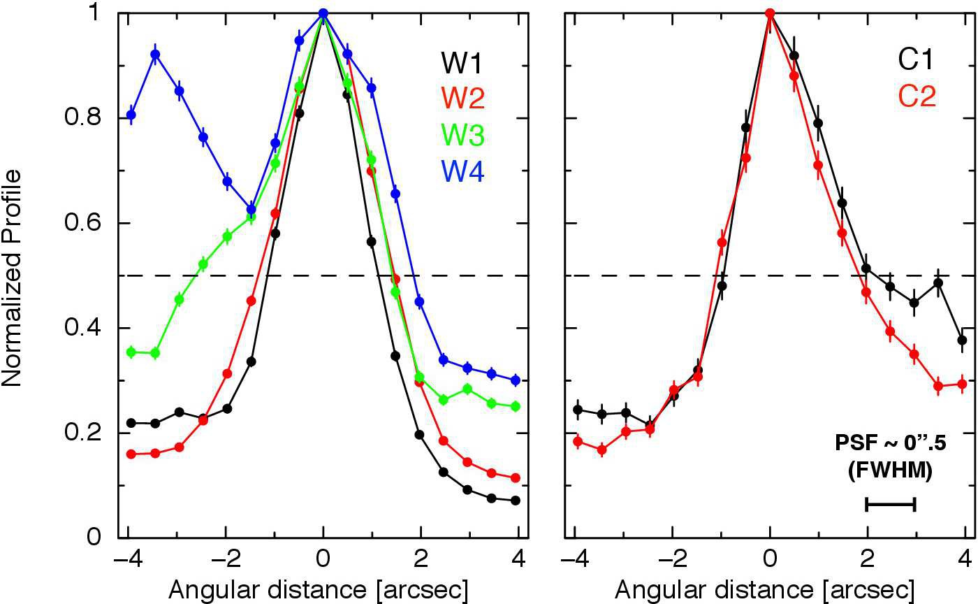
Figure 5: Emission profiles of the inward-shock filaments in the west (left) and center (right). The profiles were extracted from 15 pixels wide using 2004 image in 4.2–6 keV band and were normalized by the peak intensities. The positive direction in the angular distance shows a direction to the outside of the remnant. The scale bar in the right panel shows the Chandra’s angular resolution, $\sim$0^′′.5 (FWHM).

3.4 Thickness of the Inward-shock Filaments

We evaluate the spatial extent of the inward-shock filaments using Chandra’s high angular resolution of $\sim$0^′′.5 (FWHM). We found all filament widths to be in the range 2^′′–4^′′ (Figure 5), which is very similar to the widths of the forward-shock filaments (1^′′.5–4^′′: Vink & Laming, 2003). The angular resolution of the Wolter type-I optics used for the Chandra’s mirrors degrades at off-axis field angles. However, at the off-axis location of the inward-shock filaments (2^′–3^′), the angular resolution is nearly consistent with that at the on-axis position. Therefore, we are justified in ignoring the additional blur introduced by the off-axis effects for the shock thickness evaluation. At the remnant’s distance of 3.4 kpc, the observational thickness is estimated to be $\sim$0.03–0.07 pc. We can estimate a synchrotron loss time from the widths by combining them with the plasma fow speed away from the shock front (see section 4.2 for this discussion).

4 Discussion

We have shown that some bright filaments are moving inward with velocities of $\sim$2,100–3,800 km s^-1 using all the monitoring data taken by Chandra in 2000–2014. These filaments cannot be located at the forward-shock position even when projection is considered because the forward shock must move outward. In addition, we found that those filaments are cospatial with hard X-ray hot spots seen by NuSTAR and additionally that these filaments show flux variations (both increasing and decreasing) on timescales of a few years. These results imply that the hard X-ray emission is related to non-thermal emission from accelerated electrons at the inward-shock regions where the magnetic field is high amplified. These results hold the hope of advancing our understanding of the mysterious non-thermal X-ray emission at the interior of Cassiopeia A and the particle acceleration that is taking place at these shocks. In this section, we discuss the implications of our results on the physical conditions at the inward shocks (section 4.1), the process of particle acceleration there (section 4.2) and the origin of the inward shocks themselves (section 4.3).

4.1 Inward Shock Conditions

Here we make the plausible assumption based on the location of the inward shocks (see Figure 1) that they are propagating through the inner ejecta. Thus their actual shock velocities in the rest frame of the ejecta should be higher than what we measure from the proper motions. Here, we define the shock velocity $v_{s}$ as

$$v_{s}\equiv v_{\rm ej}-v=\frac{R_{\rm ej}}{t}-v,$$ (2)

where $v_{\rm ej}$, $v$, $R_{\rm ej}$ and $t$ are the ejecta velocity, the velocity we measure, the typical ejecta radius and the age of the remnant.

First, we consider the case where the inward shocks are propagating into cool freely-expanding ejecta. We adopt a value of $R_{\rm ej}\sim 5\times 10^{18}$ cm, which was estimated from the typical reverse shock radius at the distance of 3.4 kpc (Gotthelf et al., 2001), and then obtained an ejecta speed of $v_{\rm ej}\sim 4,900$ km s^-1 for $t\sim 320$ yr (the remnant’s age in 2000). The inward shocks have measured proper motion velocities $v$ from $-2,100$ km s^-1 to $-3,800$ km s^-1, leading to shock velocity estimates of $v_{s}\sim 7,000$–$8,700$ km s^-1. Next, we consider a case where the inward shocks are propagating into previously shocked, and therefore hot, ejecta. In this case, $v_{\rm ej}$ corresponds to the bulk expansion velocity of the ejecta. DeLaney et al. (2004) estimated an expansion rate of 0.2 % yr^-1 for the ejecta component. Using this value and the same value of $R_{\rm ej}$ as above, the expansion velocity is estimated to be $\sim$3,000 km s^-1 (see also Holt et al., 1994; Willingale et al., 2002; Morse et al., 2004; DeLaney et al., 2010, for the ejecta velocity). Now the shock velocities we infer is $v_{s}\sim 5,100$–$6,800$ km s^-1. In either case, the intrinsic shock velocity of the inward shocks is some $\sim$1–2 times higher than that of the forward shocks (4,200–5,200 km s^-1: Patnaude & Fesen, 2009).

The temperature of the medium (cool or hot plasma) into which the shock wave is propogating changes the conditions of the shock. Assuming first the cool ejecta as the medium, the sound speed (a few tens km s^-1) is much lower than the shock velocity ($\sim$7,000–8,700 km s^-1) implying a high Mach number $\mathcal{M}\gtrsim 100$. In this case, the shock compression ratio is $r=4$. On the other hand, the Mach number of the shock could be much lower, if the inward shock is propagating into hot plasma with a high sound speed. Using a typical value for the electron temperature for Cassiopeia A (2 keV, e.g., Hwang & Laming, 2012), the sound speed $c_{s}$ and Mach number $\mathcal{M}$ are estimated to be $c_{s}\sim$ 730 km s^-1 and $\mathcal{M}\sim$ 7–8 (for $v_{s}\sim 5,100$–$6,800$ km s^-1), Then the compression ratio $r=\frac{(\gamma+1)\mathcal{M}^{2}}{(\gamma-1)\mathcal{M}^{2}+2}$ is estimated to be $\sim$3.8 for $\gamma=5/3$ and $\mathcal{M}=$ 7–8, which is close to the high Mach number limit of $r=4$. In contrast, the forward shock propagates though the ISM, where both a high Mach number and high compression ratio are generally expected. We here note that effects of particle acceleration can produce a shock with a compression ratio greater $r=4$ (e.g., Berezhko & Ellison, 1999). As relativistic particles are produced and contribute significantly to the total pressure, the shocked plasma becomes more compressible ($\gamma\to$ 4/3, $r\to$ 7). Additionally the escape of the highest energy particles would also further compresses the shock by carrying off energy, analogous to that case of radiative shocks (e.g., Eichler, 1984; Berezhko & Ellison, 1999; Ellison et al., 2005).

A further complication for the shocked plasma in the remnant concerns the possibility that the electron and ion temperatures are not equilibrated. In the extreme case, the ions possess virually all of the thermal energy. Laming (2001) have calculated the time variation of the ion and electron temperatures for reverse shocks into pure oxygen ejecta for Cassiopeia A. Based on his results, we assume a plasma temperature of $\sim$ 46 keV, which is the ion temperature in the shocked plasma 150 yr after explosion. Here the sound speed $c_{s}$ and the Mach number $\mathcal{M}$ are estimated to be $c_{s}\sim$ 3,500 km s^-1 and $\mathcal{M}\sim$ 1.5–1.9. Also, the compression ratio is estimated to be $\sim$2 for $\gamma=5/3$ and $\mathcal{M}=$ 1.7. However, it is possible that particles would not accelerated in this case because the Mach number is below the critical value of $\mathcal{M}<\sqrt{5}$ for particle acceleration (Vink & Yamazaki, 2014). Columns 1 and 2 of Table 4 summarize the compression ratios and the shock velocities for the several cases we study here. Given the current state of knowledge, all of these cases offer plausible scenarios for the forward and inward shocks.

Determining the shock conditions more accurately requires measuring the ion temperatures via, e.g., thermal line broadening in the X-ray spectra. From Chandra grating spectroscopy of some bright knots (e.g., Lazendic et al., 2006), ion temperatures were estimated to be quite low (the observed lines were narrow). Therefore, the high Mach number scenario may be realistic at least for some dense features. On the other hand, for diffuse extended sources like Cassiopeia A, it is difficult to measure the line broadening accurately using grating spectroscopy. In the future, observations with a X-ray calorimeter would be more powerful. For example, the high energy resolution (FWHM $\simeq$ 5 eV) calorimeter on-board the Hitomi satellite measured line broadening of $\sim$200 km s^-1 in the Perseus cluster (Hitomi Collaboration et al., 2016, 2017) and would have revealed much about the thermal broadening in SNRs, too. We await the launch of XARM, the recovery mission for the Hitomi satellite, to reveal the shock condition more accurately in Cassiopeia A.

4.2 The Diffusion Coefficient and Particle Acceleration in Cassiopeia A

Table 4: Summary of diffusion and acceleration parameters estimated for the forward shock and the reverse shock.

	compression ratio	shock velocity	$E_{\gamma,{\rm cut},{\rm keV}}$	$B$	$k_{0}$	$E_{\rm e,max}$	$\tau_{\rm syn}$	$\tau_{\rm acc}$
forward shock
	$r=4$	4,200–5,200 km s${}^{-1~{}(2)}$	2.3 keV(1)	0.1 mG(2),(3)	1.1–1.6	34 TeV	37 yr	63 yr
	$\prime\prime$	$\prime\prime$	$\prime\prime$	0.5 mG(4)	$\prime\prime$	15 TeV	3 yr	6 yr
	$r=7$	$\prime\prime$	$\prime\prime$	0.1 mG(2),(3)	0.7–1.1	34 TeV	37 yr	63 yr
	$\prime\prime$	$\prime\prime$	$\prime\prime$	0.5 mG(4)	$\prime\prime$	15 TeV	3 yr	6 yr
inward shock
	$r=4$ (into cool ejecta)	7,000–8,700 km s${}^{-1~{}{\rm(this~{}work)}}$	1.3 keV(1)	0.5 mG${}^{\rm(5),(this~{}work)}$	5.3–8.2	11 TeV	4 yr	7 yr
	$\prime\prime$	$\prime\prime$	$\prime\prime$	1.0 mG${}^{\rm(5),(this~{}work)}$	$\prime\prime$	8 TeV	2 yr	3 yr
	$r=3.8$ (into 2 keV plasma)	5,100–6,800 km s${}^{-1~{}{\rm(this~{}work)}}$	$\prime\prime$	0.5 mG${}^{\rm(5),(this~{}work)}$	2.9–5.1	11 TeV	4 yr	7 yr
	$\prime\prime$	$\prime\prime$	$\prime\prime$	1.0 mG${}^{\rm(5),(this~{}work)}$	$\prime\prime$	8 TeV	2 yr	3 yr
	$r=2$ (into 46 keV plasma)	$\prime\prime$	$\prime\prime$	0.5 mG${}^{\rm(5),(this~{}work)}$	3.7–6.6	11 TeV	4 yr	7 yr
	$\prime\prime$	$\prime\prime$	$\prime\prime$	1.0 mG${}^{\rm(5),(this~{}work)}$	$\prime\prime$	8 TeV	2 yr	3 yr

In DSA, particles are accelerated by scattering multiple times across the shock front. Particle diffusion is characterized by the level of magnetic field turbulence. If the strength of the turbulent field is close to the unperturbed magnetic field strength (Bohm regime: $\delta B\sim B$), particles can be efficiently scattered and accelerated (see a review: Reynolds, 2008). This situation is often assumed for particle acceleration in SNRs, although it might not be so in some cases (e.g., Parizot et al., 2006; Eriksen et al., 2011). In the following we follow Parizot et al. (2006) who characterize departures from the Bohm limit as $k_{0}=D_{0}/D_{\rm 0,Bohm}$, where $D_{0}$ is the diffusion coefficient at the electron cut-off energy. This parameter can be expressed in terms of the photon cut-off energy ($E_{\gamma,cut}=h\nu_{\rm cut}$), shock velocity ($V_{3}$, in units of 1000 km s^-1) and the compression ratio $r$ as

$$k_{0}=0.14~{}E^{-1}_{\gamma,{\rm cut},{\rm keV}}~{}V^{2}_{3,{\rm shock}}~{}\frac{16(r-1)}{3r^{2}}.$$ (3)

The NuSTAR spectra above 15 keV showed photon cut-off energies for the forward shock and the reverse shock of 2.3 keV and 1.3 keV, respectively (Grefenstette et al., 2015). We here assume the shock velocity and the compression ratio at the forward shock and the inward shock listed in Table 4, which are estimated in the section 4.1. For the forward shock, the diffusion parameter was $k_{0}\lesssim$ 1.6, which is close to the Bohm regime, in both of the compression ratios ($r=4,7$). On the other hand, the inward shock shows departures from Bohm diffusion: $k_{0}\gtrsim$ 3 (Table 4). Stage et al. (2006) have already suggested a similar $k_{0}$ difference between the forward shock and the inward shock in their map of the electron cutoff frequencies in Cassiopeia A. The authors estimated upper limits to the diffusion coefficient and found that the forward-shock in the north, northeast, and southeast was close to the Bohm limit. These results agree with ours.

Using the coefficient $k_{0}$ and other observational values, we can also estimate the electron maximum energy $E_{\rm e,max}$, the synchrotron cooling timescale $\tau_{\rm syn}$ and the acceleration timescale $\tau_{\rm acc}$ as shown below (Parizot et al., 2006);

$$E_{\rm e,max}\simeq(8.3~{}{\rm TeV})\frac{4}{\sqrt{3}}\frac{\sqrt{r-1}}{r}~{}k_{0}^{-1/2}~{}B_{0.1}^{-1/2}~{}V_{\rm sh,3},$$ (4)

$$\tau_{\rm syn}\simeq(1.25\times 10^{3}~{}{\rm yr})~{}E_{\rm TeV}^{-1}~{}B_{0.1}^{-2},$$ (5)

$$\tau_{\rm acc}\simeq(30.6~{}{\rm yr})\frac{3r^{2}}{16(r-1)}~{}k_{0}~{}E_{\rm TeV}~{}B_{0.1}^{-1}~{}V_{\rm sh,3}^{-2},$$ (6)

where $B_{0.1}$ and $E_{\rm TeV}$ are the magnetic field in units of 0.1 mG and the electron energy in units of 10¹² eV, respectively. At the forward shock region, $B=$ 0.08–0.16 or 0.5 mG have been estimated by using the width of the rim of 1${}^{\prime\prime}.$5–4^′′, and also the average magnetic field in the whole SNR was estimated to be $B>$ 0.5 mG (Vink & Laming, 2003; Berezhko & Völk, 2004). For $B\gtrsim$ 0.5 mG, the synchrotron cooling timescale becomes comparable to the variability timescale of $\lesssim$ 4 yr at the reverse shock region (Uchiyama & Aharonian, 2008). Our results show almost the same timescale as that in Uchiyama & Aharonian (2008). From these observational results, we assumed the typical magnetic fields at the forward shock and the reverse shock are 0.1–0.5 mG and 0.5–1 mG, respectively. Using these parameters, we newly estimate the acceleration parameters for both the forward and inward shocks of Cassiopeia A (Table 4).

We find the maximum electron energy for the inward shock, $E_{\rm e,max}=$ 8–11 TeV to be smaller than for the forward shock ($E_{\rm e,max}=$ 15–34 TeV) even though the shock velocity at the inward shock is higher. This is because the inward shock has larger $k_{0}$ and $B$ values. The variability timescales are also estimated to be shorter at the inward shock: $\tau_{\rm syn}\sim$ 2–4 yr, $\tau_{\rm acc}\sim$ 3–7 yr (e-folding time), which is mainly due to the strong magnetic field of 0.5–1 mG. In section 3.3, we found the flux variations with timescales (for changing by $\sim$40–50 %) of $t_{\rm dec}=4\pm 1$ yr and $t_{\rm in}=9\pm 1$ yr for the W3 (and maybe also W4) region. These timescales are very similar to the predicted timescales for $B=0.5$ mG. For regions W1 and W2, the timescales were estimated to be $t_{\rm in}\sim t_{\rm dec}=4\pm 2$ yr, which is also close to the time scale for a strong magnetic field of 0.5–1 mG. For regions C1 and C2, we found gradual flux declines of $\sim$20–40 % over $\sim$14 yr. Here, $B\sim$ 0.2 mG can well explain the flux-decline timescale. From these points, we note that differences of the variability timescales can be explained by difference in the magnetic field strength. In addition, we note that the time variation of spatially adjoining regions are similar to each other (see both Figure 1 and 3). This tendency may also imply something about the difference of the magnetic field from region to region. For example, the radial positions of the inward shocks: $R_{\rm W1,W2}>R_{\rm W3,W4}>R_{\rm C1,C2}$ seems to be inversely related to the variability timescales: $t_{\rm W1,W2}<t_{\rm W3,W4}<t_{\rm C1,C2}$. This tendency might suggest that magnetic field amplification has a dependence on the radial location of the shock within the remnant. In contrast, the variability timescales at the forward shock are much longer than at the inward shock. Sato et al. (2017) have shown the time variation of X-ray flux at the forward shock region is not significant: $0.00\pm 0.07$ % yr^-1. The constant flux can be explained by the balance between acceleration and cooling even for both cases of high and low magnetic fields in Table 4 (see also Katsuda et al., 2010). We leave for future work investigations into specific scenarios to account for the rapid flux changes that we see in some of the inward shocks.

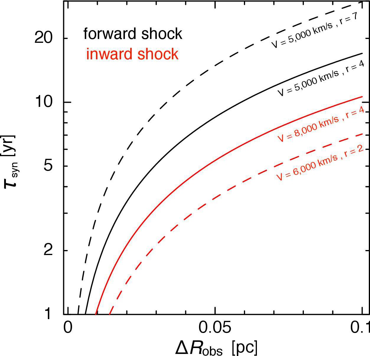
Figure 6: Synchrotron cooling timescale and observational shock width for the forward shock (black) and the inward shock (red) estimated from typical parameters in Table 4.

The synchrotron cooling timescale can be also estimated from the inward-shock width, $\sim$0.03–0.07 pc, presented in section 3.4. The accelerated electrons are advected away from the shock at a downstream velocity $V_{\rm d}=V_{\rm sh}/r$ during the synchrotron timescale, where $r$ is the shock compression ratio. The size of the advection region is thus given by $\Delta R_{\rm adv}=V_{\rm d}\times\tau_{\rm syn}$, where $\Delta R_{\rm adv}$ is the advection width. Although particle diffusion also expands the width, we simply constrain the observational width as $\Delta R_{\rm obs}\geq V_{\rm d}\times\tau_{\rm syn}\times P$, where $P$ is a projection factor. In the ideal case of a spherical shock, the projection factor is $P=4.6$. Parizot et al. (2006) described the relation between the synchrotron cooling timescale and the observational width as

$$\tau_{\rm syn}\leq\frac{\Delta R_{\rm obs}}{V_{\rm d}}\simeq(8.5~{}{\rm yr})\times\frac{r}{4}\times\bar{P}^{-1}\times V_{\rm sh,3}^{-1}\times\Delta R_{\rm obs,-2},$$ (7)

where $\bar{P}$ and $\Delta R_{\rm obs,-2}$ are defined as $\bar{P}=P/4.6$ and $\Delta R_{\rm obs}\equiv\Delta R_{\rm obs,-2}\times 10^{-2}$ pc, respectively. Using equation (7) and the estimated parameters in Table 4, the relation between the cooling time and the shock width was estimated (Figure 6). For a typical inward-shock width of 0.05 pc, the cooling timescale in the inward shock is $\lesssim$ 3–5 yr, which is consistent with the observed decay timescale and the predicted cooling timescale in the case of $B=$ 0.5–1 mG (Table 4). For the forward shock, the timescale is longer ($\sim$10 yr) than that for the inward shock. This tendency is the same as the other observational timescale estimates (Table 4).

Particle acceleration at reverse shocks have been studied in some theoretical work (e.g., Ellison et al., 2005; Telezhinsky et al., 2012, 2013). For all of the models, the maximum energy reached by particles at the reverse shock is always lower than at the forward shock. Also, recent deep $\gamma$-ray observations of Cassiopeia A with MAGIC have showed a clear exponential cut-off at $\sim$ 3.5 TeV (Guberman et al., 2017), which implies only modest cosmic-ray acceleration to very high energy for the hadronic scenario. From the observations, Cassiopeia A is considered not to be a PeVatron (PeV accelerator) at its present age. Both theoretical and observational studies suggest that particle acceleration at the reverse shock (inward shock) in Cassiopeia A could not produce the high energy particles (protons) up to “knee” energy ($\sim 3\times 10^{15}$ eV) even if the shock has as high a shock velocity as shown in section 4.1. On the other hand, the reverse shock region is propogating into a metal-rich environment produced by supernova nucleosynthesis. If such elements were accelerated by the reverse shocks, the cosmic-ray composition would be affected. Therefore, particle acceleration at reverse shocks are important for understanding the cosmic-ray abundances.

4.3 The Origin of the Inward Shocks

For SNR expansion into an ambient medium with a constant or gradually declining density profile (e.g., ISM, CSM), it is not possible to explain an inward moving reverse shock (in the observer frame) for an evolutional phase that describes Cassiopeia A. In such a young evolutionary phase, the reverse shock must expand outward. As an alternative explanation for the inward shocks we consider a “reflection shock” produced by the forward shock interacting with a density jump in the ambient medum.

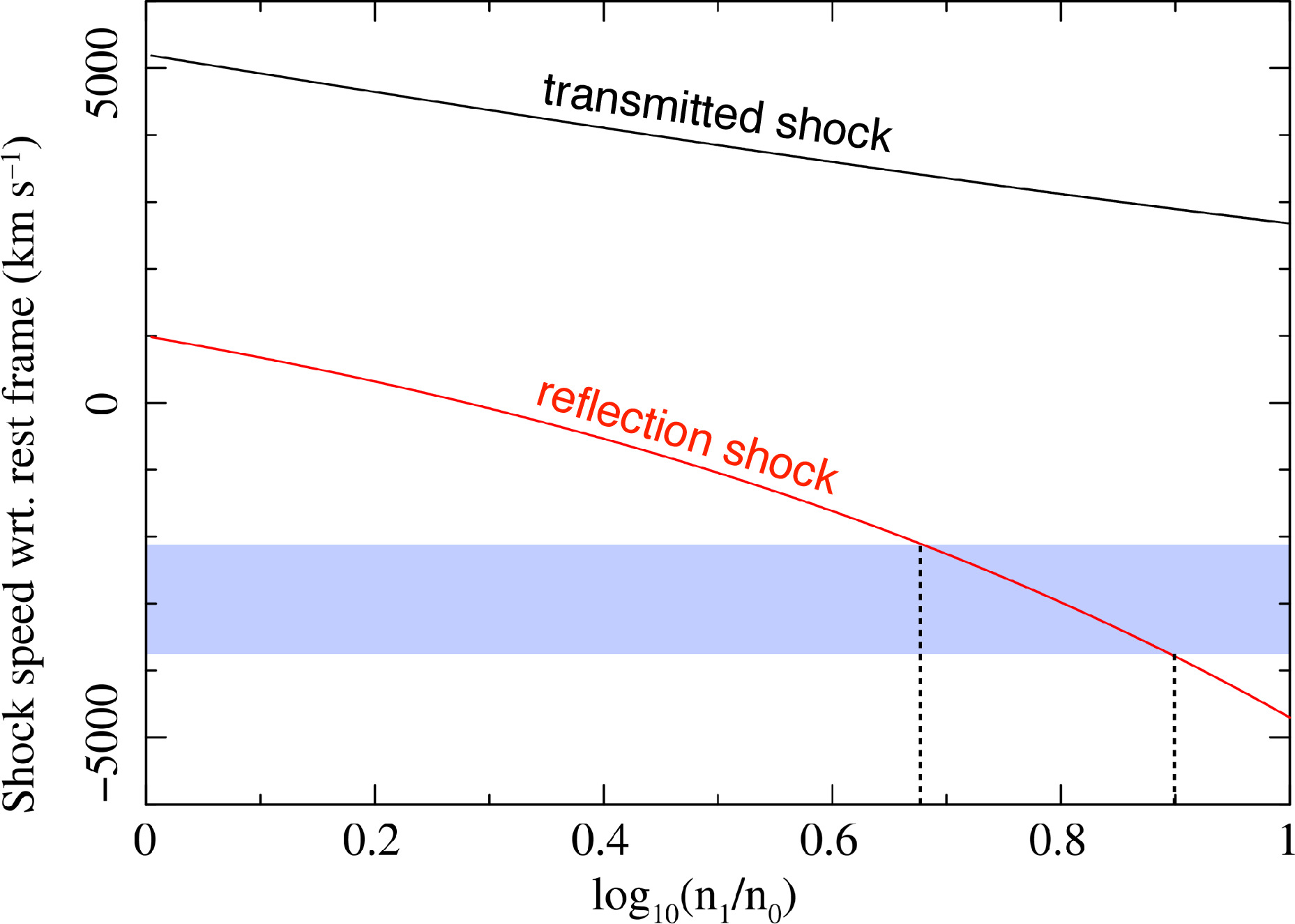
Figure 7: Estimate of the reflection shock velocity and the density of interacting cloud in the case of Cassiopeia A with solving the fluid equation in Hester et al. (1994). The black and red curve show the velocities of the transmitted shock (that is propagating through the cloud) and reflection shock, respectively. Blue area shows the range of the velocities of the western filaments in this work: $\sim$2,100–3,800 km s^-1.

The reflection-shock conditions can be calculated using a simple fluid equation (Hester et al., 1994). We here assume a density of ambient medium before the encounter with the density jump as $\rho_{0}$. The density jump $\rho_{1}$ is defined as $\rho_{1}\equiv\alpha\rho_{0}$. Then, the forward shock density $\rho_{2}$ is described as $\rho_{2}=4\rho_{0}$ from the Rankine–Hugoniot relation. After the encounter, a contact discontinuity is made by the interaction. Upward materials are compressed by $4\rho_{1}$, and then downward materials are pushed back (see also Inoue et al., 2012). Figure 7 shows the estimate of the reflection shock speed using Hester et al. (1994). We assumed the forward shock is interacting with the density jump with the speed of 5,200 km s^-1. In order to explain the inward-shock velocities, we require that the forward shock be interacting with a surrounding material whose density is $\gtrsim$ 5-8 times higher than that of a ambient medium elsewhere.

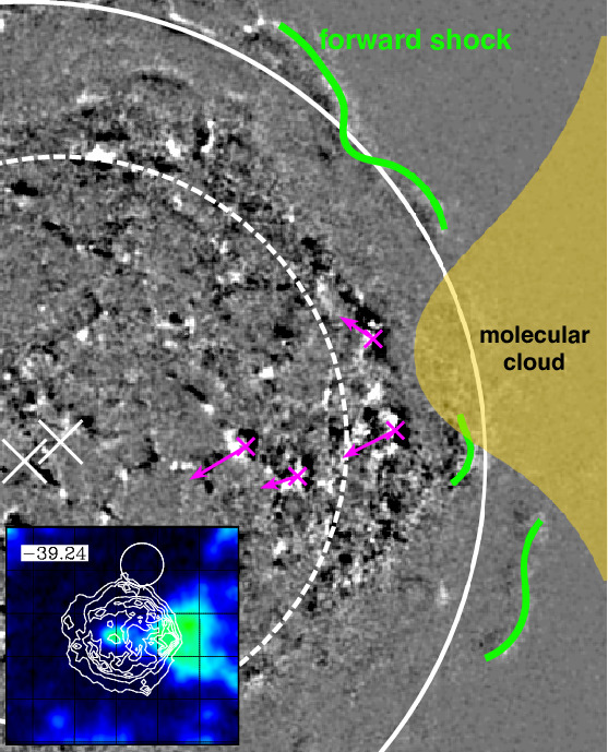
Figure 8: A schematic diagram of the shock-cloud interaction. The image show the same image as in Figure 1(a). Magenta arrows show the proper-motion directions of the inward shocks. The forward shocks are emphasized by thick green lines. Small and large circles indicate the radii of the reverse shock and forward shock (Gotthelf et al., 2001), respectively. Cross marks show the center positions of each circle. The center of the reverse-shock circle offsets to the northeast direction. Small screen set on left bottom show the CO map with the velocity of $-39.24$ km s^-1 in Kilpatrick et al. (2014). A distance between the reverse shock and the forward shock is $\sim$ 0.7 pc at the western region.

A local molecular cloud would be a good candidate for explaining such an enhanced density structure around the remnant. Millimeter observations in ¹²CO and ¹³CO J = 2–1 (230 and 220 GHz) with the Heinrich Hertz Submillimeter Telescope indicated the existence of the molecular cloud around Cassiopeia A (Kilpatrick et al., 2014). In particular, the inward-shock regions seems to overlay with the fastest gas ($-50$ to $-45$ km s^-1) and the slowest gas ($-39$ to $-34$ km s^-1). We show a schematic diagram of the shock-cloud interaction in Figure 8. As shown in this figure, the inward shocks seems to be shifting radially against the distribution of the molecular clouds. Here, we can estimate the time when the forward shock first hits the cloud and pushes the reflection shock into the ejecta. Dividing the distance between the forward shock and the inward shocks ($\sim$ 0.7 pc, see Figure 8) by their velocity difference of $\sim$ 7000 km s^-1, it can be estimated to be $<$ 100 yrs ago. This is much shorter than the age of the remnant ($\sim$ 350 yrs old), providing us with a further support that the inward shocks are reflection shocks by the western cloud. Not only the western filaments but also the filaments at the central position (e.g., C1, C2) might be also related to the shock-cloud interaction. For example, the high-speed CO gas ($-46$ to $-49$ km s^-1) is concentrated in filamentary structure to the south and southeast of the remnant. The locations are very close to the positions of the central inward shocks (see Figure 3 right in Kilpatrick et al., 2014).

However, it is difficult to confirm the shock-cloud interaction. Kilpatrick et al. (2014) have argued for a shock-cloud interaction around the western and southern rim using the broadened CO lines (see Fig. 4 in Kilpatrick et al., 2014). As a matter of fact, their locations are a little different from the inward-shock positions. Future observations with the Nobeyama 45-m Telescope will be helpful in studying the shock interaction with the molecular cloud. ¹²CO observations with the telescope would have good spatial resolution ($\sim 17^{\prime\prime}$) able to reveal more small structures and the relation with the X-ray distributions (Inaba et al., private communication). For example, in the case of RX J1713.7–3946, non-thermal X-rays which are enhanced around CO and H_I clumps have been found (e.g., Sano et al., 2010, 2013, 2015). They suggested that the amplified magnetic field around the CO and H_I clumps enhances the synchrotron X-rays and possibly the acceleration of cosmic-ray electrons. In the theoretical view, the amplified magnetic field could be explained as one of features of the shock-cloud interaction. Inoue et al. (2012) have investigated cosmic-ray acceleration assuming interaction with clumpy interstellar clouds using three-dimensional magnetohydrodynamic simulations. They predicted a highly amplified magnetic field of $\sim$1 mG caused by a turbulent shell due to the shock-cloud interactions. Then, the short-time X-ray variability was predicted at the same time. This supports well our observational results in Cassiopeia A as discussed in the section 4.2.

5 Conclusion

The bright non-thermal X-ray emission in the interior of Cassiopeia A has been one of the most enigmatic features of the remnant since the earliest observations by Chandra. Even as basic a fact as the type of shock (e.g., forward shock, reverse shock or something else) has remained obscure. In this paper, we put forth new evidence that the interior non-thermal emission originates in an “inward shock” through new analyses of archival Chandra and NuSTAR observations. We identified inward moving filaments in the remnant’s interior using monitoring data by Chandra from 2000 to 2014. The inward-shock positions are spatially coincident with the most intense hard (15–40 keV band) X-ray emission seen with NuSTAR.

We measured the proper motions of the inward shocks, which equate to speeds of $\sim$2,100–3,800 km s^-1 for a distance of 3.4 kpc to the remnant. Assuming the shocks are propagating through the expanding ejecta (which is itself moving outward), we determine that the shock velocities in the frame of the ejecta could reach up to $\sim$5,100–8,700 km s^-1, which is $\sim$ 1–2 times higher than that at the forward shock. Additionally some of the inward-shock filaments showed flux variations (both increasing and decreasing) on timescales of just a few years. We find that the high shock velocity combined with a high magnetic field strength ($\sim$ 0.5–1 mG) in the reverse shock region can explain the non-thermal properties well. At the same time we are able to constrain the diffusion coefficient and find that diffusion at the reverse shock is less efficient ($k_{0}\gtrsim$3) than that of the forward shock ($k_{0}\lesssim$ 1.6). Expressed in terms of magnetic field turbulence, we find (as do others) that the turbulence at the forward shock approaches the Bohm limit, while at the inward shocks turbulence is less well developed.

As to the nature of the inward shocks, we propose that they are “reflection shocks” caused by the forward shock’s interaction with a density enhancement in the circumstellar medium. A density jump of a factor of $\gtrsim$5–8 reproduces the observed inward-shock velocities. Previous works have shown evidence for a local molecular cloud on the western side of Cassiopeia A with some indications of an interaction beyween the cloud and the remnant’s shock. Further investigations into the shock-cloud interaction will be useful to deepen our understanding of particle acceleration in Cassiopeia A.

Appendix A Rice Distribution

In our study we determined the magnitude of proper motion $\mu$ and its direction $\theta$ from measurements along the RA and decl. axes. To sufficient accuracy we can approximate our measurements as normally distributed in $X$ and $Y$ with means of $\mu\cos(\theta)$ and $\mu\sin(\theta)$ and variances of $\sigma^{2}$. This formulation assumes that the uncertainties are the same in both directions. Our naive estimate for the proper motion, $p=(X^{2}+Y^{2})^{1/2}$, follows the Rice distribution (see also Appendix I in Serkowski, 1958), which has a probability density function (PDF) given by

$$f(p)={p\over\sigma^{2}}\exp\left(-\frac{p^{2}+\mu^{2}}{2\sigma^{2}}\right)I_{0}\left(\frac{p\mu}{\sigma^{2}}\right)$$ (A1)

where $I_{0}$ is the modified Bessel function of the first kind with order zero. This distribution function is bounded at zero and is asymmetric, especially when $\mu/\sigma^{2}$ is small. Hence the naive estimate for the magnitude of proper motion just introduced is biased high. In order to account for this bias, we use the Rice PDF.

The mean of the Rice PDF is

$$\langle\mu\rangle=\sigma\sqrt{\pi/2}\,\exp(-\mu^{2}/2\sigma^{2})\,_{1}F_{1}(3/2;1;\mu^{2}/2\sigma^{2}),$$ (A2)

where ${}_{1}F_{1}$ is the confluent hypergeometric function. This can be expressed in terms of Bessel functions (e.g., Talukdar & Lawing, 1991) as

$$\langle\mu\rangle=\sigma\sqrt{\pi/2}\,e^{-x/2}\,\left[(1+x)I_{0}(x/2)+xI_{1}(x/2)\right]$$ (A3)

with $x=\mu^{2}/2\sigma^{2}$. The variance of the Rice distribution is given by

$$\sigma^{2}_{\langle\mu\rangle}=2\sigma^{2}+\mu^{2}-\langle\mu\rangle^{2}.$$ (A4)

To obtain an unbiased estimate for the proper notion we solve Eq. (A3) for $\mu$ by setting $p=\langle\mu\rangle$. Eq. (A4) is then used to determine the uncertainty on the proper motion.

References

- Acciari et al. (2010) Acciari, V. A., Aliu, E., Arlen, T., et al. 2010, ApJ, 714, 163
- Ackermann et al. (2013) Ackermann, M., Ajello, M., Allafort, A., et al. 2013, Science, 339, 807
- Aharonian et al. (2001) Aharonian, F., Akhperjanian, A., Barrio, J., et al. 2001, A&A, 370, 112
- Albert et al. (2007) Albert, J., Aliu, E., Anderhub, H., et al. 2007, A&A, 474, 937
- Anderson & Rudnick (1995) Anderson, M. C., & Rudnick, L. 1995, ApJ, 441, 307
- Arnaud (1996) Arnaud, K. A. 1996, Astronomical Data Analysis Software and Systems V, 101, 17
- Bamba et al. (2005) Bamba, A., Yamazaki, R., Yoshida, T., Terasawa, T., & Koyama, K. 2005, ApJ, 621, 793
- Bell (1978) Bell, A. R. 1978, MNRAS, 182, 443
- Berezhko & Ellison (1999) Berezhko, E. G., & Ellison, D. C. 1999, ApJ, 526, 385
- Berezhko & Völk (2004) Berezhko, E. G., & Völk, H. J. 2004, A&A, 419, L27
- Blandford & Eichler (1987) Blandford, R., & Eichler, D. 1987, Phys. Rep., 154, 1
- Cash (1979) Cash, W. 1979, ApJ, 228, 939
- DeLaney et al. (2004) DeLaney, T., Rudnick, L., Fesen, R. A., et al. 2004, ApJ, 613, 343
- DeLaney et al. (2010) DeLaney, T., Rudnick, L., Stage, M. D., et al. 2010, ApJ, 725, 2038
- Eichler (1984) Eichler, D. 1984, ApJ, 277, 429
- Ellison et al. (2005) Ellison, D. C., Decourchelle, A., & Ballet, J. 2005, A&A, 429, 569
- Eriksen et al. (2011) Eriksen, K. A., Hughes, J. P., Badenes, C., et al. 2011, ApJ, 728, L28
- Farnebäck (2003) Farnebäck, G. 2003, Springer, “Two-frame motion estimation based on polynomial expansion”, “Image Analysis”, pages 363-370.
- Fesen et al. (2006) Fesen, R. A., Hammell, M. C., Morse, J., et al. 2006, ApJ, 645, 283
- Fruscione et al. (2006) Fruscione, A., McDowell, J. C., Allen, G. E., et al. 2006, Proc. SPIE, 6270, 62701V
- Gotthelf et al. (2001) Gotthelf, E. V., Koralesky, B., Rudnick, L., et al. 2001, ApJ, 552, L39
- Grefenstette et al. (2014) Grefenstette, B. W., Harrison, F. A., Boggs, S. E., et al. 2014, Nature, 506, 339
- Grefenstette et al. (2015) Grefenstette, B. W., Reynolds, S. P., Harrison, F. A., et al. 2015, ApJ, 802, 15
- Grefenstette et al. (2017) Grefenstette, B. W., Fryer, C. L., Harrison, F. A., et al. 2017, ApJ, 834, 19
- Guberman et al. (2017) Guberman, D., Cortina, J., de Oña Wilhelmi, E., et al. 2017, arXiv:1709.00280
- Harrison et al. (2013) Harrison, F. A., Craig, W. W., Christensen, F. E., et al. 2013, ApJ, 770, 103
- Helder & Vink (2008) Helder, E. A., & Vink, J. 2008, ApJ, 686, 1094
- Hester et al. (1994) Hester, J. J., Raymond, J. C., & Blair, W. P. 1994, ApJ, 420, 721
- Hitomi Collaboration et al. (2016) Hitomi Collaboration, Aharonian, F., Akamatsu, H., et al. 2016, Nature, 535, 117
- Hitomi Collaboration et al. (2017) Hitomi Collaboration, Aharonian, F., Akamatsu, H., et al. 2017, arXiv:1711.00240
- Holt et al. (1994) Holt, S. S., Gotthelf, E. V., Tsunemi, H., & Negoro, H. 1994, PASJ, 46, L151
- Hughes et al. (2000) Hughes, J. P., Rakowski, C. E., Burrows, D. N., & Slane, P. O. 2000, ApJ, 528, L109
- Hwang et al. (2000) Hwang, U., Holt, S. S., & Petre, R. 2000, ApJ, 537, L119
- Hwang et al. (2004) Hwang, U., Laming, J. M., Badenes, C., et al. 2004, ApJ, 615, L117
- Hwang & Laming (2012) Hwang, U., & Laming, J. M. 2012, ApJ, 746, 130
- Inoue et al. (2012) Inoue, T., Yamazaki, R., Inutsuka, S.-i., & Fukui, Y. 2012, ApJ, 744, 71
- Jokipii (1987) Jokipii, J. R. 1987, ApJ, 313, 842
- Katsuda et al. (2010) Katsuda, S., Petre, R., Mori, K., et al. 2010, ApJ, 723, 383
- Keohane et al. (1996) Keohane, J. W., Rudnick, L., & Anderson, M. C. 1996, ApJ, 466, 309
- Kilpatrick et al. (2014) Kilpatrick, C. D., Bieging, J. H., & Rieke, G. H. 2014, ApJ, 796, 144
- Koyama et al. (1995) Koyama, K., Petre, R., Gotthelf, E. V., et al. 1995, Nature, 378, 255
- Laming (2001) Laming, J. M. 2001, ApJ, 563, 828
- Lazendic et al. (2006) Lazendic, J. S., Dewey, D., Schulz, N. S., & Canizares, C. R. 2006, ApJ, 651, 250
- Maeda et al. (2009) Maeda, Y., Uchiyama, Y., Bamba, A., et al. 2009, PASJ, 61, 1217
- Morse et al. (2004) Morse, J. A., Fesen, R. A., Chevalier, R. A., et al. 2004, ApJ, 614, 727
- Patnaude & Fesen (2007) Patnaude, D. J., & Fesen, R. A. 2007, AJ, 133, 147
- Patnaude & Fesen (2009) Patnaude, D. J., & Fesen, R. A. 2009, ApJ, 697, 535
- Patnaude et al. (2011) Patnaude, D. J., Vink, J., Laming, J. M., & Fesen, R. A. 2011, ApJ, 729, L28
- Patnaude & Fesen (2014) Patnaude, D. J., & Fesen, R. A. 2014, ApJ, 789, 138
- Parizot et al. (2006) Parizot, E., Marcowith, A., Ballet, J., & Gallant, Y. A. 2006, A&A, 453, 387
- Reed et al. (1995) Reed, J. E., Hester, J. J., Fabian, A. C., & Winkler, P. F. 1995, ApJ, 440, 706
- Reynolds (2008) Reynolds, S. P. 2008, ARA&A, 46, 89
- Sano et al. (2010) Sano, H., Sato, J., Horachi, H., et al. 2010, ApJ, 724, 59
- Sano et al. (2013) Sano, H., Tanaka, T., Torii, K., et al. 2013, ApJ, 778, 59
- Sano et al. (2015) Sano, H., Fukuda, T., Yoshiike, S., et al. 2015, ApJ, 799, 175
- Sanders (2006) Sanders, J. S. 2006, MNRAS, 371, 829
- Sato et al. (2017) Sato, T., Maeda, Y., Bamba, A., et al. 2017, ApJ, 836, 225
- Sato & Hughes (2017a) Sato, T., & Hughes, J. P. 2017a, ApJ, 840, 112
- Sato & Hughes (2017b) Sato, T., & Hughes, J. P. 2017b, ApJ, 845, 167
- Serkowski (1958) Serkowski, K. 1958, Acta Astron., 8, 135
- Stage et al. (2006) Stage, M. D., Allen, G. E., Houck, J. C., & Davis, J. E. 2006, Nature Physics, 2, 614
- Talukdar & Lawing (1991) Talukdar, K. K., & Lawing, W. D. 1991, Acoustical Society of America Journal, 89, 1193
- Telezhinsky et al. (2012) Telezhinsky, I., Dwarkadas, V. V., & Pohl, M. 2012, A&A, 541, A153
- Telezhinsky et al. (2013) Telezhinsky, I., Dwarkadas, V. V., & Pohl, M. 2013, A&A, 552, A102
- Uchiyama et al. (2007) Uchiyama, Y., Aharonian, F. A., Tanaka, T., Takahashi, T., & Maeda, Y. 2007, Nature, 449, 576
- Uchiyama & Aharonian (2008) Uchiyama, Y., & Aharonian, F. A. 2008, ApJ, 677, L105
- Vink & Laming (2003) Vink, J., & Laming, J. M. 2003, ApJ, 584, 758
- Vink & Yamazaki (2014) Vink, J., & Yamazaki, R. 2014, ApJ, 780, 125
- Williams et al. (2017) Williams, B. J., Coyle, N. M., Yamaguchi, H., et al. 2017, ApJ, 842, 28
- Willingale et al. (2002) Willingale, R., Bleeker, J. A. M., van der Heyden, K. J., Kaastra, J. S., & Vink, J. 2002, A&A, 381, 1039