Themis-ml:

Abstract

As more industries integrate machine learning into socially sensitive decision processes like hiring, loan-approval, and parole-granting, we are at risk of perpetuating historical and contemporary socioeconomic disparities. This is a critical problem because on the one hand, organizations who use but do not understand the discriminatory potential of such systems will facilitate the widening of social disparities under the assumption that algorithms are categorically objective. On the other hand, the responsible use of machine learning can help us measure, understand, and mitigate the implicit historical biases in socially sensitive data by expressing implicit decision-making mental models in terms of explicit statistical models. In this paper we specify, implement, and evaluate a “fairness-aware” machine learning interface called themis-ml, which is intended for use by individual data scientists and engineers, academic research teams, or larger product teams who use machine learning in production systems.

1 Introduction

In recent years, the transformative potential of machine learning (ML) in many industries has propelled ML into the forefront of mainstream media. From improving products and services to optimizing logistics and operations, ML and artificial intelligence more broadly offer a wide range of tools for organizations to enhance their internal and external capabilities.

As with any tool, we can use ML to engender great social benefit, but as [1] emphasizes, we can also misuse it to bring about devastating harm. In this paper, we focus on ML systems in the context of Decision Support Systems (DSS), which are software systems that are intended to assist humans in various decision-making contexts [2, 3, 4, 5]. The misuse of ML in these types of systems could potentially precipitate a widespread adverse impact on society by introducing insidious feedback loops between biased historical data and current decision-making [1].

Researchers have developed many discrimination discovery and fairness-aware ML methods [6, 7, 8, 9, 10, 11, 12, 13], so we build on work done by others and seek to leverage these techniques in the context of research- and product-based machine learning applications.

Our contributions in this paper are three-fold. First, we propose an application programming interface (API) for “Fairness-aware Machine Learning Interfaces” (FMLI) in the context of a simple binary classifier. Second, we introduce themis-ml, an FMLI-compliant library, and apply it to a hypothetical loan-granting DSS using the German Credit Dataset [14]. Finally, we evaluate the efficacy of themis-ml as a tool for measuring potential discrimination (PD) in both training data and ML predictions as well as mitigating PD using fairness-aware methods. Our hope is that themis-ml serves as a reference implementation that others might use and extend for their own purposes.

2 Bias and Discrimination

Colloquially, bias is simply a preference for or against something, e.g. preferring vanilla over chocolate ice cream. While this definition is intuitive, here we explicitly define algorithmic bias as a form of bias that occurs when mathematical rules favor one set of attributes over others in relation to some target variable, like “approving” or “denying” a loan.

Algorithmic bias in machine learning models can occur when a trained model systematically generates predictions that favor one group over another in relation to some set of attributes, e.g. education, and some target variable, e.g. “default on credit”. While the definition above of bias is amoral, discrimination is in essence moral, occurring when an action is based on biases resulting in the unfair treatment of people. We define fairness as the inverse of discrimination, meaning that a “fairness-aware” model is one that produces non-discriminatory predictions.

Bias can lead to either direct (intended/explicit) or indirect (unintended/implicit) discrimination, and the predominant legal concepts used to determine these two types are known as disparate treatment and disparate impact, respectively [15]. As [6, 7] suggest, we can address disparate treatment in ML models by simply removing all variables that are highly correlated to the protected class of interest, in addition to the protected class itself, from the training data. However, as [6] points out, doing so does not necessarily mitigate discriminatory predictions and may actually introduce unfairness into an otherwise fair system. In contrast, addressing disparate impact is more complex because it depends on historical processes that generated the training data, non-linear relationships between the features and protected class, and whether we are interested in measuring individual- or group-level discrimination [12].

3 A Fairness-aware Machine Learning Interface

So how does one measure disparate impact and individual-/group-level discrimination in an ML-driven product? In this section, we describe the main components of a simple classification system, enumerate a few of the use cases that a research or product team might have for using an FMLI, and propose an API that fulfills these use cases.

A simple classification ML pipeline consists of five steps: data ingestion, data preprocessing, model training, model evaluation, and prediction generation on new examples. Data ingestion is outside the scope of this paper because it is a highly variable process that depends on the application, often involves considerable engineering effort, and potentially requires external stakeholder buy-in.

Table 1 outlines a simple classification system in terms of the core interfaces in scikit-learn (sklearn), which is a machine learning library in the Python programming language [16], and table 2 delineates some of the use cases that research or product teams might have to justify the use of an FMLI.

Table 1: A Simple Classification Pipeline

API Interface	Function	Examples
Transformer	Preprocess raw data for model training.	mean-unit variance scaling, min-max scaling
Estimator	Train models to perform a classification task.	logistic regression, random forest
Scorer	Evaluate performance of different models.	accuracy, f1-score, area under the curve
Predictor	Predict outcomes for new data.	single-classifier prediction, ensemble prediction

4 FMLI Specification

Here we propose a high-level specification of themis-ml, an open source FMLI named after the ancient Greek titaness of justice (the library can be found on github.) We adopt sklearn’s principles of consistency, inspection, non- proliferation of classes, composition, and sensible defaults [16], and extend them with the following FMLI-specific principles:

.15in1 Model flexibility. Focus on fairness-aware methods that are applicable to a variety of model types because users might have no control or full control over the specific model training implementation. .15in1 Fairness as performance. Provide estimators and scoring metrics that explicitly encode a notion of both model accuracy and fairness so that models can optimize for both. .15in1 Transparency of fairness-utility tradeoff. Fair models often make less accurate predictions [8, 13], which is an important factor when assessing their business impact.

Table 2: FMLI Use Cases

Use Case	Rationale
Detect and reduce discrimination in a production machine learning pipeline.	Fairness-aware modeling aligns with team/company values, provides protection from legal liability.
Measure individual-/group-level discrimination in data with respect to a protected class and outcome of interest.	Need to assess the potential bias resulting from training models on data.
Preprocess raw data or post-process model predictions in a way that reduces discriminatory predictions generated by models.	Unable to change the underlying implementation of the model training process.
Explicitly learn model parameters that produce fair predictions for a variety of model types.	Need for flexibility when experimenting with or deploying different model types.
Evaluate the degree to which fairness-aware methods reduce discrimination and assess the fairness-utility tradeoff.	Need for assessing the business consequences or other implications of deploying a fairness-aware model.

4.1 Preliminaries

In the following subsections we describe specific methods from the ML fairness literature that map onto each of the sklearn interfaces. Note that we only provide a high level summary of each method, citing the original sources for more implementation details. The following descriptions make two assumptions: (i) the positive target label $y^{+}$ refers to a desirable outcome, e.g. “approve loan”, and vice versa for the negative target label $y^{-}$, and (ii) the protected class is a binary variable defined as $s\in\{d,a\}$, where $X_{d}$ are members of the disadvantaged group and $X_{a}$ are members of the advantaged group.

Following these conventions, we define $X_{d,y^{+}}$ and $X_{d,y^{-}}$ as the set of observations of the disadvantaged group that are positively labelled and negatively labelled, respectively. Similarly, $X_{a,y^{+}}$, and $X_{a,y^{-}}$ are observations of the advantaged group that are positively and negatively labelled, respectively.

4.2 Transformer

The main idea behind fairness-aware preprocessing is to take a dataset $D$ consisting of a feature set $X_{train}$, target labels $y_{train}$, and protected class $s_{train}$ to output a modified dataset.

Relabelling, also called Massaging, modifies $y_{train}$ by relabelling the target variables in such a way that “promotes” members of the disadvantaged protected class (e.g. “immigrant”) and “demotes” members of the advantaged class (e.g. “citizen”) [7]. A ranker $R$ (e.g. logistic regression) is trained on $D$, and ranks are generated for all observations. Some of the top-ranked observations $X_{d,y^{-}}$ are “promoted” to $X_{d,y^{+}}$ and some of the bottom-ranked observations $X_{a,y^{+}}$ are “demoted” to $X_{a,y^{-}}$ such that the proportion of $y^{+}$ are equal in both $X_{d}$ and $X_{a}$. Two caveats of this method are that it is intrusive because it directly manipulates $y$, and that it narrowly defines fairness as the uniform distribution of benefits between $X_{a}$ and $X_{d}$.

⬇ from themis_ml.preprocess import Relabeller from sklearn.linear_model import LogisticRegression \par# use logistic regression as the ranking algorithm massager = Relabeller(ranker=LogisticRegression) \par# obtain a new set of labels new_y = massager.fit_transform(X, y, s) \par# train any model on new y labels lr = LogisticRegression() lr.fit(X, new_y) Reweighting takes a dataset D and assigns a weight to each observation using conditional probabilities based on $y$ and $s$ [7]. In brief, large weights are assigned to $X_{d,y^{+}}$ and $X_{a,y^{-}}$ , while small weights are assigned to $X_{d,y^{-}}$ and $X_{a,y^{+}}$. The weights are then used as input to model types that support weighted sample observations — which actually points to the main limitation of this method, since not all classifiers can incorporate observation weights during the learning process. ⬇ from themis_ml.preprocess import Reweight from sklearn.linear_model import LogisticRegression \parreweigher = Reweight() \par# obtain fairness-aware weights for each observation reweigher.fit(y, s) fair_weights = reweigher.transform(y, s) \par# train a LogisticRegression model with sample weights lr = LogisticRegression() lr.fit(X, y, weights=fair_weights) Sampling is composed of two methods: the first involves uniformly sampling n observations from each group, where n is the expected size of that group assuming a uniform distribution. The second is to preferentially sample observations using a ranker $R$, similar to the Relabelling method. The procedure is to duplicate the top-ranked $X_{d,y^{+}}$ and $X_{a,y^{-}}$ while removing top-ranked $X_{d,y^{-}}$ and $X_{a,y^{+}}$ [7]. ⬇ from themis_ml.preprocess import ( UniformSample, PreferentialSample) from sklearn.linear_model import LogisticRegression \par# use logistic regression as the ranking algorithm uniform_sampler = UniformSample() preferential_sampler = PreferentialSample( ranker=LogisticRegression) \par# obtain a new dataset with uniform sampling uniform_sampler.fit(y_train, s_train) X, y, s = uniform_sampler.transform(X, y, s) \par# obtain a new dataset with preferential sampling preferential_sampler.fit(y_train, s_train) X, y, s = preferential_sampler.transform(X, y, s)

4.3 Estimator

Themis-ml implements two methods for training fairness-aware models: the prejudice remover regularizer (PRR), and the additive counterfactually fair (ACF) model. [8] proposes PRR as an optimization technique that extends the standard L1/L2-norm regularization method [17, 18] by adding a prejudice index term to the objective function. This term is equivalent to normalized mutual information, which measures the degree to which predictions $y$ and $s$ are dependent on each other. With values ranging from 0 to 1, 0 means that $y$ and $s$ are independent, and a value of 1 means that they are dependent. The goal of the objective function is to find model parameters that minimize the difference between the true label $y$ and the predicted label $\hat{y}$ in addition to the degree to which $y$ depends on s. ⬇ from themis_ml.linear_model import LogisticRegressionPRR \par# use L2-norm regularization and prejudice index as # the discrimination penalizer lr_prr = LogisticRegressionPRR( penalty="L2", discrimination_penalty="PI") \par# fit the models lr_prr.fit(X, y, s) ACF is a method described by [6] within the framework of counterfactual fairness. The main idea is to train linear models to predict each feature using the protected class attribute(s) as input. We can then compute the residuals $\epsilon_{ij}$ between the predicted feature values and true feature values for each observation i and each feature j. The final model is then trained on $\epsilon_{ij}$ as features to predict y. ⬇ from themis_ml.linear_model import LinearACFClassifier \par# by default, LinearACFClassifier uses linear # regression as the continuous feature estimator # and logistic regression as the binary feature # estimator and target variable classifier linear_acf = LinearACFClassifier() \par# fit the models linear_acf.fit(X_train, y_train, s_train)

4.4 Predictor

Themis-ml draws on two methods to make model type-agnostic predictions: Reject Option Classification (ROC) and Discrimination Aware Ensemble Classification (DAEC) [9]. Unlike the Transformer and Estimator methods outlined above, ROC and DAEC do not modify the training data or the training process. Rather, they postprocess predictions in a way that reduces potentially discriminatory (PD) predictions. [9] describes two ways of implementing ROC, starting with ROC in a single classifier setting. ROC works by training an initial classifier on $D$, generating predicted probabilities on the test set, and then computing the proximity of each prediction to the decision boundary learned by the classifier. Within this boundary defined by the critical region threshold $\theta$, where 0.5 < $\theta$ < 1, $X_{d}$ are assigned as $y^{+}$ and $X_{a}$ are assigned as $y^{-}$. ROC in the multiple classifier setting is similar to the single classifier setting, except that predicted probabilities are defined as the weighted average of probabilities generated by each classifier. ⬇ from themis_ml.postprocessing import ( SingleROClassifier, MultiROClassifier) from sklearn.linear_model import LogisticRegression from sklearn.tree import DecisionTreeClassifier \par# use logistic regression for single classifier setting single_roc = SingleROClassifier( estimator=LogisticRegression()) \par# use logistic regression and decision trees for # multiple classifier setting multi_roc = MultiROClassifier( estimators=[LogisticRegression(), DecisionTreeClassifier()]) \par# fit the models and generate predictions single_roc.fit(X, y, s) multi_roc.fit(X, y, s) single_roc.predict(X, s) multi_roc.predict(X, s) The main limitation of ROC is that model types must be able to produce predicted probabilities. DAEC gets around this problem by training an ensemble of classifiers and, through a similar relabelling rule as ROC, re-assigns any prediction where classifiers disagree on the predicted label. As [9] notes, in general, the larger the disagreement between classifiers, the larger the reduction in discrimination. ⬇ from themis_ml.postprocessing import DAEnsembleClassifier from sklearn.linear_model import LogisticRegression from sklearn.tree import DecisionTreeClassifier \par# use logistic regression and decision trees dae_clf = DAEnsembleClassifier( estimators=[LogisticRegression(), DecisionTreeClassifier()]) \par# fit the models and generate predictions dae_clf.fit(X, y, s) dae_clf.predict(X, s)

4.5 Scorer

The Scorer interface is concerned with measuring the degree to which data or predictions are PD. Themis-ml implements two methods for measuring group-level discrimination and two methods for measuring individual-level discrimination. In the context of measuring group-level discrimination, [13] describes mean difference and normalized mean difference. Mean difference measures the difference between $p(a\cup y^{+})$ and $p(d\cup y^{+})$. Values range from -1 to 1, where -1 is the reverse-discrimination case (all $X_{a}$ have $y^{-}$ labels and all $X_{d}$ have $y^{+}$ labels) and 1 is the fully discriminatory case (all $X_{a}$ have $y^{+}$ labels and all $X_{d}$ have $y^{-}$ labels). Normalized mean difference, which also takes on values between -1 and 1, scales these values based on the maximum possible discrimination in a dataset given the rate of positive labels [13]. ⬇ from themis_ml.metrics import ( mean_difference, normalized_mean_difference) \par# compare group-level discrimination in true # labels and predicted labels md_y_true = mean_difference(y, s) md_y_pred = mean_difference(pred, s) md_y_pred - md_y_true \parnorm_md_y_true = norm_mean_difference(y, s) norm_md_y_pred = norm_mean_difference(pred, s) norm_md_y_pred - norm_md_y_true [13] also describes consistency and situation test score as individual-level discrimination measures. Consistency measures the difference between the target label of a particular observation and target labels of its neighbors. K-nearest neighbors (knn) measures the pairwise distance between observations X. Then, for each observation $x_{i}$ and each neighbor $(x_{j},y_{j})\in knn(x_{i})$, we compute the differences between $y_{i}$ and target labels of neighbor $y_{j}$. A consistency score of 0 indicates that there is no individual-level discrimination, and a score of 1 indicates that there is maximum discrimination in the dataset. The situation test score metric is similar to consistency, except we consider only $x_{i}\in X_{d}$. This method uses mean difference to compute a discrimination score among neighbors $x_{j}\in knn(x_{i})$, producing a score between 0 and 1, where 0 indicates no discrimination, and 1 indicates maximum discrimination [13]. ⬇ from themis_ml.metrics import ( consistency, situation_test_score) \par# compare individual-level discrimination # in true labels and predicted labels c_true = consistency(y, s) c_pred = consistency(y, s) c_pred - c_true \parsts_true = situation_test_score(y, s) sts_pred = situation_test_score(y, s) sts_pred - sts_true

5 Evaluating Themis-ml

In this section we use the German Credit dataset [14] to evalute themis-ml. We use mean difference as the “fairness” measure and the area under the curve (AUC) as the “utility” measure. The former represents the degree to which PD patterns in $D$ are learned by the ML model, and the latter represents the predictive power of a model given the available dataset $(X,y,s)\in D$. The following analysis is by no means meant to be a comprehensive investigation of all possible workflows that themis- ml enables. However, does demonstrate the potential of themis-ml as a tool that facilites fairness-aware machine learning by enabling the user to: 1. Measure PD target label distributions in the training data. 2. Measure PD predicted labels in a machine learning algorithm’s predictions. 3. Reduce PD predictions using fairness-aware techniques. 4. Diagnose the fairness-utility tradeoff in a particular data context. The German Credit dataset classifies 1000 anonymized individuals as having “good” and “bad” credit risks as part of a bank loan application, which we encode as $1$ and $0$ respectively to define the credit risk target variable. Each individual is associated with twenty attributes such as the purpose of the loan, employment status, and other personal information. We begin the analysis by extracting three protected class attributes — female, foreign worker, and age below 25 — and encode them as binary variables such that the putatively disadvantaged group is encoded as $1$, and the advantaged group is encoded as $0$ (the advantaged group would be male, citizen worker, and age above 25, respectively). Using the Scorer interface, we measure PD patterns with respect to credit risk and each of the protected classes defined above using the mean difference and normalized mean difference metrics. Table 3 reports the PD distribution of “good” and “bad” credit risks with respect to the protected attributes female, foreign worker, and age below 25. The fact that both the mean difference (md) and normalized mean difference (nmd) scores are greater than zero suggests that the probability of being classified as having “good” risk is higher in the advantaged group than that of the disadvantaged group. Table 3: Potentially discriminatory target variable distribution. md = mean difference, nmd = normalized mean difference. protected class md (%) md 95% CI nmd (%) nmd 95% CI female 7.48 (1.35, 13.61) 7.73 (1.39, 14.06) foreign worker 19.93 (4.91, 34.94) 63.96 (15.76, 112.17) age below 25 14.94 (7.76, 22.13) 17.29 (8.97, 25.61)

5.1 Experimental Procedure

To assess the extent to which (i) a model trained on these data mirrors these PD credit risk distributions, and (ii) fairness-aware techniques can reduce these methods, we used mean difference to measure model fairness and AUC to measure model utility. For this experiment we specify five conditions: • Baseline (B): Train a model on all available input variables in the German Credit dataset, including protected attributes. • Remove Protected Attribute (RPA): Train a model on input variables without protected attributes. This is the naive fairness-aware approach. • Relabel Target Variable (RTV): Train a model using the Relabelling fairness-aware method. • Counterfactually Fair Model (CFM): Train a model using the Additive Counterfactually Fair method. • Reject-option Classification (ROC): Train a model using the Reject-option Classification method. For each of these conditions, we train LogisticRegression, DecisionTree, and RandomForest model types using 10-fold cross validation; generate train and test predictions; and compute AUC and mean difference metrics for each train-test pair. We then compute the mean of these metrics for each condition and model type. The code for this analysis is available on github.

5.2 Measuring and Mitigating Potentially Discriminatory Predictions

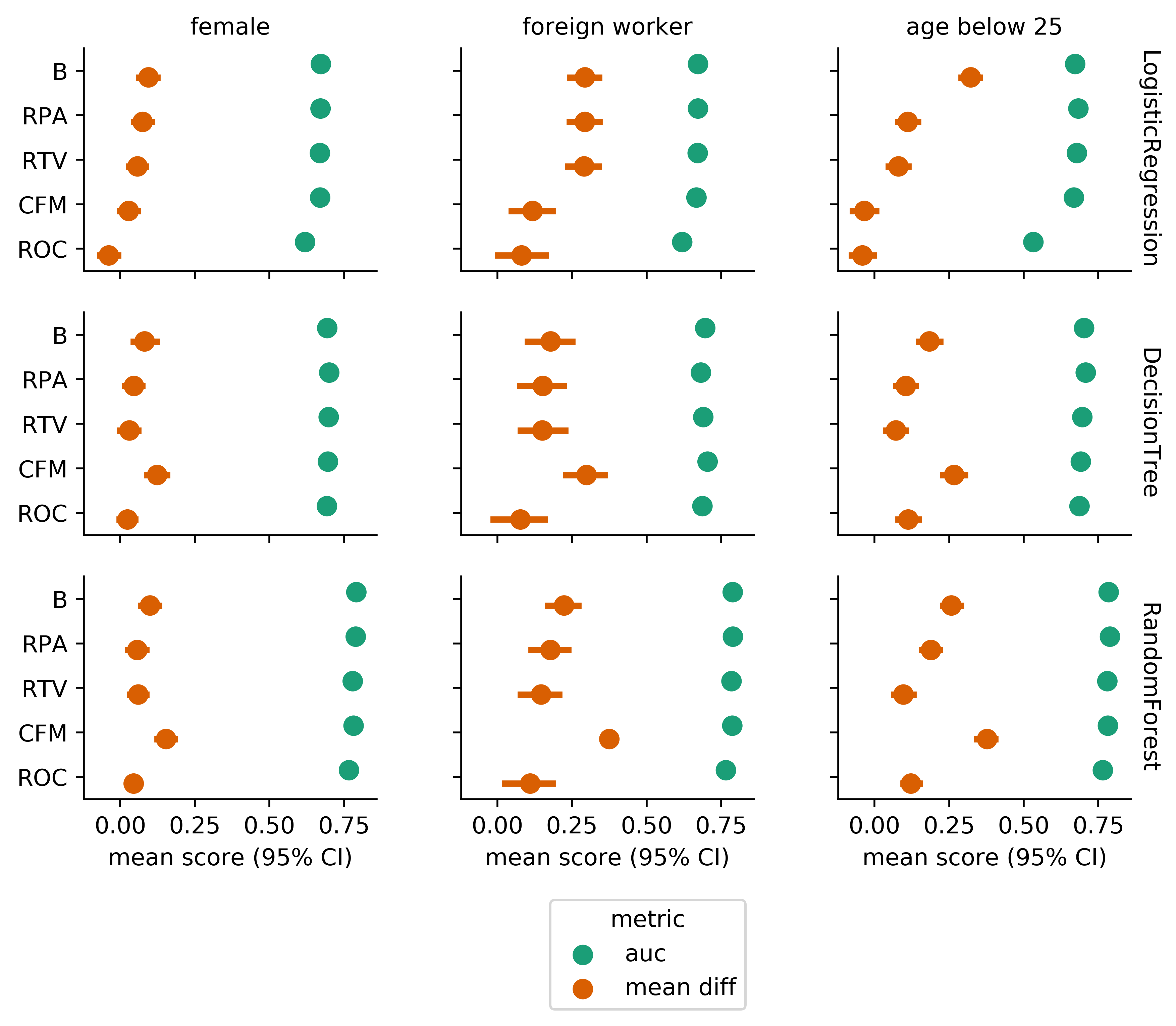
Figure 1: Comparison of Fairness-aware Methods using LogisticRegression, DecisionTree, and RandomForest (rows) as base estimators for each protected attribute context (columns), measured by AUC and mean difference evaluated on test set predictions. Figure 1 suggests that in the case of LogisticRegression, the baseline model B does indeed mirror the PD patterns found in the true target variable. Furthermore, each of the fairness-aware methods appear to have the desired effect of reducing mean difference, but to varying degrees depending on the method and protected attribute. In the female protected attribute context, where there appears to be the least PD (mean difference of $7.48\%$), the reductive effect of the fairness-aware methods do not appear to be as large as in the foreign worker and age below 25 contexts. The lack of reduction in mean difference between B and RPA, with respect to foreign worker and LogisticRegression, illustrates the observation made by [6] that removing protected attributes from the training data does not necessarily prevent the algorithm from mirroring PD patterns in the data. However, the sizeable reduction in mean difference between B and RPA, with respect to age below 25 and LogisticRegression model, shows that removing protected attributes can sometimes make models more fair while also retaining predictive power. An interesting thing to note here is that the Additive Counterfactually Fair method actually increases mean difference for DecisionTrees and RandomForests across all protected attribute contexts. Two possible explanations behind this observation is that certain assumptions made by ACF are not suitable for non-linear learning algorithms, or the meta-estimators that compute the residuals for non-linear estimators should be non-linear as well. This is an open question worth future inquiry.

5.3 The Fairness-utility Tradeoff

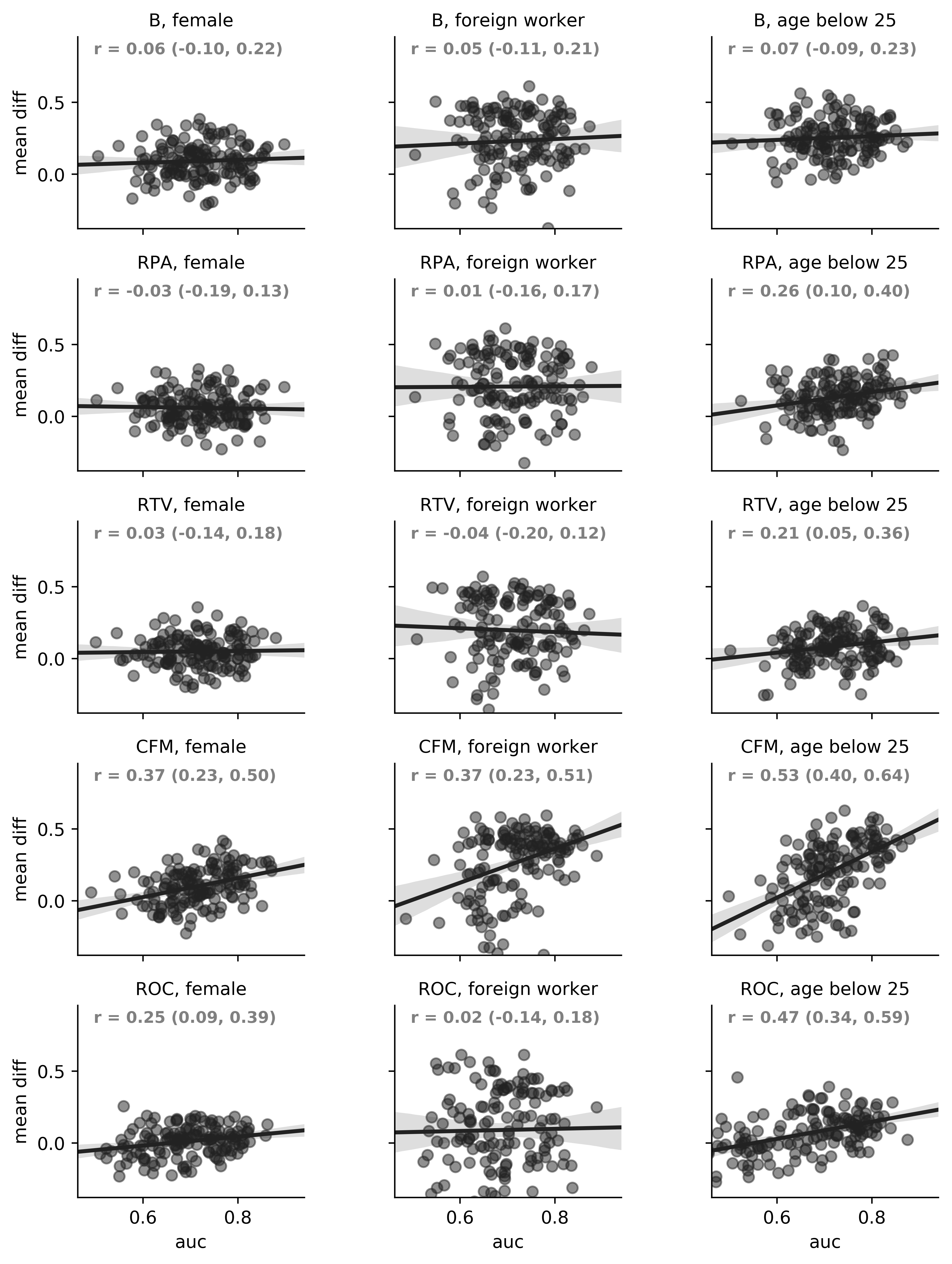
Just as the bias-variance tradeoff has become a useful diagnostic tool to guide ML research and application [19], the fairness- utility tradeoff can help machine learning practitioners and researchers determine which fairness-aware methods are suitable for their particular data context. Figure 2: Correlation between AUC and Mean Difference for each fairness-aware condition (rows) and protected attribute contexts (columns) across all model types (LogisticRegression, DecisionTree, RandomForest). 95% confidence intervals are provided for the pearson $r$ correlation metric. In figure 2, we visualize the fairness-utility tradeoff, in this case as measured by mean difference and AUC, respectively. We report pearson correlation coefficients $r$ for each protected attribute context and fairness-aware condition with their respective 95% confidence intervals. These results suggest that the relationship between fairness and utility is noisy, however there does seem to be a consistent but weak positive correlation between mean difference and AUC (or a negative correlation between fairness and utility, since lower scores are better for mean difference and higher scores are better for AUC). Interestingly, we note the cases in which there are zero or negative $r$ coefficient values. $r=0$ implies that there is no tradeoff between fairness and utility: one can expect to increase the utility of a set of models without adversely affecting the fairness of predictions generated by those models. Although there are no cases where $r_{ci\ upper}<0$, $r<0$ suggests that it might be plausible to find regimes in which one can expect to increase both the utility and fairness of a model. Future work in this area might examine the asymptotic behavior of the relationship between fairness and utility as model complexity increases. Depending on one’s use cases, analyses like this might prove to be a useful guide for figuring out what kinds of methods are robust in the sense that one can reduce PD predictions with little to no adverse impact on predictive performance.

6 Discussion

In this paper, we describe and evaluate an FMLI in the classification context where we consider only a single binary protected class variable and a binary target variable. More work needs to be done to generalize FMLIs to the multi-classification, regression, and multiple protected classes settings. Furthermore, many basic questions about model tuning, evaluation, and selection in the fairness-aware context remain. For instance, what might be some reasonable ways to aggregate utility and fairness metrics in order to find the optimal set of hyperparameters? Additionally, little is understood about the composability of fairness-aware methods, i.e., when different techniques are used together in sequence, are the resulting discrimination reductions additive or otherwise? Future technical work might also extend the FMLI specification to include techniques like Locally Interpretable Model-Agnostic Explanations [18] and develop legal frameworks for thinking about how different stakeholders would interact with FMLIs. For example, companies that choose not to expose the model-training components of their internal ML pipeline could still grant some form of access to the predictions generated by the models if there were to be a set of standards for model transparency and accountability. Finally, many of the fairness-aware methods, such as the Relabeller, implicitly define fairness as the uniform (equal) distribution of benefits among disadvantaged and advantaged groups. Future work would make this definition more flexible, for example, by defining fairness as the proportional distribution of benefits based on need. This would necessitate the mathematical formalization of another set of assumptions about the needs of disadvantaged and advantaged groups. Given the challenges ahead, our ability to measure and mitigate discrimination is limited by our common social, legal, and political understanding of fairness itself. This common understanding is often lacking because marginalized social groups typically do not have a voice at the table when defining what counts as fair. Since FMLIs are simply a tool to measure and mitigate formalized definitions of discrimination, it is important for all stakeholders to engage in an inclusive forum where everyone, especially disadvantaged social groups, can contribute.

- [1] C. O’Neil, Weapons of math destruction: How big data increases inequality and threatens democracy. Broadway Books, 2017.
- [2] M. Yoshimura, Y. Fujimi, K. Izui, and S. Nishiwaki, “Decision-making support system for human resource allocation in product development projects,” International Journal of Production Research, vol. 44, no. 5, pp. 831–848, 2006.
- [3] A. A. Montgomery, T. Fahey, T. J. Peters, C. MacIntosh, and D. J. Sharp, “Evaluation of computer based clinical decision support system and risk chart for management of hypertension in primary care: randomised controlled trial,” Bmj, vol. 320, no. 7236, pp. 686–690, 2000.
- [4] G. O. Barnett, J. J. Cimino, J. A. Hupp, and E. P. Hoffer, “Dxplain: an evolving diagnostic decision-support system,” Jama, vol. 258, no. 1, pp. 67–74, 1987.
- [5] J. Mysiak, C. Giupponi, and P. Rosato, “Towards the development of a decision support system for water resource management,” Environmental Modelling & Software, vol. 20, no. 2, pp. 203–214, 2005.
- [6] M. J. Kusner, J. R. Loftus, C. Russell, and R. Silva, “Counterfactual fairness,” arXiv preprint arXiv:1703.06856, 2017.
- [7] F. Kamiran and T. Calders, “Data preprocessing techniques for classification without discrimination,” Knowledge and Information Systems, vol. 33, no. 1, pp. 1–33, 2012.
- [8] T. Kamishima, S. Akaho, H. Asoh, and J. Sakuma, “Fairness-aware classifier with prejudice remover regularizer,” Machine Learning and Knowledge Discovery in Databases, pp. 35–50, 2012.
- [9] F. Kamiran, A. Karim, and X. Zhang, “Decision theory for discrimination-aware classification,” in Data Mining (ICDM), 2012 IEEE 12th International Conference on, pp. 924–929, IEEE, 2012.
- [10] R. Zemel, Y. Wu, K. Swersky, T. Pitassi, and C. Dwork, “Learning fair representations,” in Proceedings of the 30th International Conference on Machine Learning (ICML-13), pp. 325–333, 2013.
- [11] M. B. Zafar, I. Valera, M. Gomez Rodriguez, and K. P. Gummadi, “Fairness constraints: Mechanisms for fair classification,” arXiv preprint arXiv:1507.05259, 2017.
- [12] C. Dwork, M. Hardt, T. Pitassi, O. Reingold, and R. Zemel, “Fairness through awareness,” in Proceedings of the 3rd Innovations in Theoretical Computer Science Conference, pp. 214–226, ACM, 2012.
- [13] I. Zliobaite, “A survey on measuring indirect discrimination in machine learning,” arXiv preprint arXiv:1511.00148, 2015.
- [14] K. Bache and M. Lichman, “Uci machine learning repository [http://archive.ics.uci.edu/ml]. irvine, ca: University of california, school of information and computer science. begleiter, h. neurodynamics laboratory. state university of new york health center at brooklyn. ingber, l.(1997). statistical mechanics of neocortical interactions: Canonical momenta indicatros of electroencephalography,” Physical Review E, vol. 55, pp. 4578–4593, 2013.
- [15] S. Barocas and A. D. Selbst, “Big data’s disparate impact,” 2016.
- [16] L. Buitinck, G. Louppe, M. Blondel, F. Pedregosa, A. Mueller, O. Grisel, V. Niculae, P. Prettenhofer, A. Gramfort, J. Grobler, et al., “Api design for machine learning software: experiences from the scikit-learn project,” arXiv preprint arXiv:1309.0238, 2013.
- [17] A. Y. Ng, “Feature selection, l 1 vs. l 2 regularization, and rotational invariance,” in Proceedings of the twenty-first international conference on Machine learning, p. 78, ACM, 2004.
- [18] M. T. Ribeiro, S. Singh, and C. Guestrin, “Why should i trust you?: Explaining the predictions of any classifier,” in Proceedings of the 22nd ACM SIGKDD International Conference on Knowledge Discovery and Data Mining, pp. 1135–1144, ACM, 2016.
- [19] S. Fortmann-Roe, “Understanding the bias-variance tradeoff,” 2012.
- [20] B. Bischl, M. Lang, L. Kotthoff, J. Schiffner, J. Richter, E. Studerus, G. Casalicchio, and Z. M. Jones, “mlr: Machine learning in r,” Journal of Machine Learning Research, vol. 17, no. 170, pp. 1–5, 2016.
- [21] M. Y. Park and T. Hastie, “L1-regularization path algorithm for generalized linear models,” Journal of the Royal Statistical Society: Series B (Statistical Methodology), vol. 69, no. 4, pp. 659–677, 2007.