The First APOKASC Catalog of Kepler Dwarf and Subgiant Stars

Abstract

We present the first APOKASC catalog of spectroscopic and asteroseismic data for dwarfs and subgiants. Asteroseismic data for our sample of 415 objects have been obtained by the Kepler mission in short, 58.5 s, cadence and lightcurves span from 30 up to more than 1000 days. The spectroscopic parameters are based on spectra taken as part of the Apache Point Observatory Galactic Evolution Experiment (APOGEE) and correspond to Data Release 13 of the Sloan Digital Sky Survey. We analyze our data using two independent $T_{\rm eff}$ scales, the spectroscopic values from DR13 and those derived from SDSS griz photometry. We use the differences in our results arising from these choices as a test of systematic temperature uncertainties, and find that they can lead to significant differences in the derived stellar properties. Determinations of surface gravity ($\log{g}$), mean density ($\langle\rho\rangle$), radius ($R$), mass ($M$), and age ($\tau$) for the whole sample have been carried out by means of (stellar) grid-based modeling. We have thoroughly assessed random and systematic error sources in the spectroscopic and asteroseismic data, as well as in the grid-based modeling determination of the stellar quantities provided in the catalog. We provide stellar properties determined for each of the two $T_{\rm eff}$ scales. The median combined (random and systematic) uncertainties are 2% (0.01 dex; $\log{g}$), 3.4% ($\langle\rho\rangle$), 2.6% ($R$), 5.1% ($M$), and 19% ($\tau$) for the photometric $T_{\rm eff}$ scale and 2% ($\log{g}$), 3.5% ($\langle\rho\rangle$), 2.7% ($R$), 6.3% ($M$), and 23% ($\tau$) for the spectroscopic scale. We present comparisons with stellar quantities in the asteroseismic catalog by Chaplin et al. (2014) that highlight the importance of having metallicity measurements for determining stellar parameters accurately. Finally, we compare our results with those coming from a variety of sources, including stellar radii determined from TGAS parallaxes and asteroseismic analyses based on individual frequencies. We find a very good agreement for all inferred quantities. The latter comparison, in particular, gives a strong support to the determination of stellar quantities based on global seismology, a relevant result for future missions such as TESS and PLATO.

1 Introduction

The advent of space-borne asteroseismology of stars showing solar-like oscillations has been instrumental in the dawning of the era of precision stellar astrophysics. First CoRoT (Michel et al., 2008; De Ridder et al., 2009) and then Kepler (Gilliland et al., 2010; Bedding et al., 2010; Chaplin et al., 2010) have provided a novel way to determine precise stellar parameters – most importantly mean density ($\langle\rho\rangle$), surface gravity ($\log{g}$), mass ($M$), radius ($R$), and age ($\tau$) – for large numbers of stars.

The capability that asteroseismology offers for the determination of stellar parameters requires knowledge of effective temperature ($T_{\rm eff}$) but stellar ages in particular are sensitive to the metallicity, and to some extent even to the mixture of heavy elements. In turn, composition information is also necessary to enable stellar and galactic studies. Stellar spectroscopy is thus essential for realizing the full potential of asteroseismology. Pinsonneault et al. (2014) produced the first catalog of asteroseismically derived stellar parameters for red giant stars based on asteroseismic data from Kepler and from the high-resolution Apache Point Observatory Galactic Evolution Experiment (APOGEE), part of the Sloan Digital Sky Survey (SDSS). This first APOKASC catalog included more than 1916 stars observed as part of the SDSS-DR10 (Ahn et al., 2014). When completed, the full APOKASC catalog will contain about 15,000 stars.

Other surveys focused on the Kepler or CoRoT fields include the SAGA survey (Casagrande et al., 2014, 2016) that has observed the Kepler field with Strömgren photometry with DR1 containing about 1,000 stars and CoRoGEE, the combination of APOGEE and CoRoT, a combined dataset of 606 red giant stars (Chiappini et al., 2015; Anders et al., 2017). These efforts have now been extended to include the fields of the Kepler extended mission K2 (Howell et al., 2014; Lund et al., 2016; Stello et al., 2017), with large-scale observation campaigns being carried out by APOGEE (Zasowski et al. in prep.), Galah (De Silva et al., 2015, Sharma et al. in prep.), LAMOST (Zhao et al., 2012), and RAVE (Valentini et al., 2017).

Most of the activity related to large scale surveys is focused on red giant stars, as their larger oscillation amplitudes and brightness, and their longer oscillation periods, make them much easier targets for asteroseismology. Joint asteroseismic and spectroscopic analysis of the smaller dwarf and subgiant samples, however, remains important. First, the spatial distribution of the dwarf sample is much more confined to the solar neighborhoold ($\sim$300 pc) than the giant sample ($\sim$2000 pc Huber et al., 2014 or even further than 4000 pc for the faint giants Mathur et al., 2016). Properties, such as the age-metallicity and age-velocity disperson relations, can then be readily compared to such pioneering work as Edvardsson et al. (1993) and Nordström et al. (2004). The sources of systematic error can therefore be investigated; hence bridging results out to the regions sampled by the giants from stars where we have the most accurate independent observations (parallax, interferometry, etc).

Stellar parameters of dwarf and subgiant stars can be determined best from asteroseismic measurements when frequencies of many individual oscillation modes can be measured precisely and matched by stellar models. Lebreton & Goupil (2014) discusses in detail different approaches for using frequency data. Recent examples based on Kepler targets include: 42 main sequence and subgiant stars (Appourchaux et al., 2012; Metcalfe et al., 2014), 33 exoplanet host stars (Davies et al., 2016; Silva Aguirre et al., 2015). More recently, (Lund et al., 2017; Silva Aguirre et al., 2017) have analyzed the LEGACY sample, composed by 66 stars that have Kepler light curves longer than 1 year. These samples overlap. The LEGACY sample includes some of the stars in Metcalfe et al. (2014), while works by Bellinger et al. (2016); Creevey et al. (2017) are based on seismic data from (Davies et al., 2016) and the LEGACY sample. In contrast, global seismic parameters, namely the large frequency separation ($\Delta\nu$) and the frequency of maximum power ($\nu_{\rm max}$) that are closely related to $\langle\rho\rangle$ and $\log{g}$, are available for a much larger number of dwarfs and subgiants. Kepler has provided $\Delta\nu$ and $\nu_{\rm max}$ for more than 500 main sequence and subgiant stars and determinations of stellar properties were initially reported by Chaplin et al. (2011b), based on the Kepler Input Catalog $T_{\rm eff}$ and ${\rm[Fe/H]}$ values. The first catalog for this sample including stellar ages, based on more accurate and precise photometric $T_{\rm eff}$ determinations, but still lacking ${\rm[Fe/H]}$ measurements for the whole sample, was later on presented in Chaplin et al. (2014, hereafter C14).

A subset of our sample allows us to critically compare the results from detailed modeling of individual frequencies with those from scaling relations relative to the Sun. We also, crucially, have detailed abundance data on the stars in our sample, which was not true in C14, and we have $T_{\rm eff}$ estimates from photometry and spectroscopy for the whole sample for the first time. Both of these advantages justify the presentation of a revised catalog including this new APOGEE data.

In this work, we present the extension of the APOKASC catalog (Pinsonneault et al., 2014) to include 415 dwarf and subgiant stars that form a homogeneous sample with the previously released and also future red giants catalog. Spectroscopic parameters are determined from spectra released in SDSS-III DR10 but with data extracted using the methods of SDSS-IV DR13 (Albareti et al. 2016, Holtzmann et al. 2017 in prep.). The catalog includes newly determined global seismic parameters obtained from Kepler short-cadence light curves, improving over those used in C14 both because of longer duration lightcurves and in the analysis techniques (Handberg & Lund, 2014). In Section 2 we describe the sample and the spectroscopic and asteroseismic data and analysis methods. Section 3 presents the grid-based modeling (GBM) approach used to determine stellar parameters for the catalog while Section 4 is devoted to the determination of errors and central values for the catalog. Section 5 presents the information contained in the catalog and comparison with previous work. A summary is presented in Section 6. Finally, two appendices include detailed information about stellar models and extensive comparisons among GBM pipelines used in this work.

2 The Sample

The catalog consists of stars with detected solar-like oscillations in Kepler short-cadence data as reported in Chaplin et al. (2011a) and with spectroscopic observations from the APOGEE-1 survey (Majewski et al., 2015). APOGEE-1 observed 415 out of the $\sim\,600$ stars in Chaplin et al. (2011a). Stars with photometric temperature estimates higher than 6500 K were de-prioritized because the IR spectra from APOGEE were not expected to be informative for such hot targets. There were also other targeting constraints as summarized by Zasowski et al. (2013). For our purposes, the most important were that the APOGEE field of view is slightly smaller than a Kepler CCD module, therefore objects that fell on the corners of a Kepler CCD module were not observed. In addition, targets that fell within $\sim$70 arcseconds of another target could be discarded in favor of the higher priority giant target. Finally, APOGEE-1 had already completed its observations of certain parts of the Kepler field when the dwarf targets were added.

The APOGEE survey is a bright-time component of the Sloan Digital Sky Survey III (Eisenstein et al., 2011). Using the Sloan Foundation Telescope (Gunn et al., 2006) at Apache Point Observatory, APOGEE observed 230 science targets simultaneously across a 7 deg² field of view in the standard observing mode. An additional 35 fibers were devoted to standard stars and 35 fibers to sky. 300 fibers fed the APOGEE spectrograph (Wilson et al., 2012). APOGEE spectra cover the $H$-band, between 1.51 $\mu$m and 1.7 $\mu$m, at a resolution R=22,500.

2.1 Spectroscopic analysis

APOGEE data is reduced in a three-step process. Initially, observations of an individual plate on an individual night are reduced taking into account: the calibration of the detector, detection of bad pixels, wavelength calibration, dither shifts between exposures in a visit, correction of individual exposures and determination of radial velocity of each object by using a best-matching stellar template. The second step combines multiple individual visits to the same objects: it corrects for each visit-specific radial velocity and coadds the spectra. The final spectra are resampled onto a fixed wavelength grid with constant dispersion in $\log{\lambda}$. Details can be found in Nidever et al. (2015).

The final step, extraction of stellar parameters and chemical abundances, is done by the APOGEE Stellar Parameters and Chemical Abundances pipeline (ASPCAP). Here we summarize its main characteristics.

ASPCAP performs $\chi^{2}$ minimization over grids of precomputed synthetic spectra (e.g. Zamora et al. 2015). The basic parameter space search is performed over $T_{\rm eff}$, $\log{g}$, [M/H], ${\rm\alpha/M}$, to which C, N, line broadening and/or microturbulence can be added. The optimization is done with FERRE (Allende Prieto et al., 2006), which performs a $\chi^{2}$ minimization by comparing fluxes as a function of wavelength with weights that come directly from the uncertainties in the fluxes determined during data reduction. Synthetic spectra across the grids are constructed by interpolation of model fluxes for spectra computed at the nodes of the grid. This is more robust than interpolating atmospheric structures and then computing the synthetic spectra from the interpolated structure (Mészáros et al., 2013). A detailed description of how ASPCAP works can be found in García Pérez et al. (2016).

Once ASPCAP has determined the best-fit stellar parameters to the grid of synthetic spectra, these parameters are compared to external values of high accuracy (”ground truth”) and, if necessary, a calibration relation is applied to bring the ASPCAP values into agreement with ground truth. For this work, seismic measurements provide accurate gravities, but the calibration of the ASPCAP temperatures and metallicities are relevant. For $T_{\rm eff}$, the comparision values are based on $J-K$ colors and the color-Teff relation of González Hernández & Bonifacio (2009). For metallicity, the comparison values are the mean metallicities of well-studied clusters. Details about how the calibration samples were constructed are available in Holtzman et al. (2015) for DR12 and Holtzman et al. (2017, in preparation) for DR13.

2.1.1 Preliminary analysis with modified DR12 parameters

The APOGEE stellar parameters and abundances released prior to Data Release 13 (DR13) were derived assuming that stellar rotation was a negligible contribution to line-broadening at the resolution of the APOGEE spectra. Therefore, the synthetic spectra grid used for $\chi^{2}$ minimization was not convolved with stellar rotation broadening profiles. While this assumption is usually appropriate for giants, which are the majority of the stars observed by APOGEE, warmer dwarfs ($T_{\rm eff}\gtrsim$ 6000K) and younger dwarfs of all temperatures can still show noticeable rotation even at APOGEE resolution. This was realized at an early stage of this project, during the preparation of DR12, so a modified pipeline was developed to correct for this effect by adding rotation velocity as another dimension in the grid of atmosphere models. When rotation is included in the optimization procedure, C and N are fixed to solar values, i.e. ${\rm[C/Fe]=0}$ and ${\rm[N/Fe]=0}$, to keep the computational needs constrained.

The DR12-rot spectroscopic parameters were used in combination with asteroseismic data (Sect. 2.2) by all the Grid-Based Modeling pipelines (GBMs; see Sect. 3) to carry out comparisons among the codes. The offsets and different standard deviations found in these comparisons do not depend on whether we adopt the DR12-rot or the DR13 spectroscopic values.

2.1.2 DR13

The final ASPCAP spectroscopic parameters used in the catalog correspond to DR13 (Albareti et al., 2016). DR13 includes by default a grid of models including rotation for dwarfs, an improved relation between microturbulence and gravity, and a relation for macroturbulence. Some of the improvements brought about by DR13 are discussed in (Albareti et al., 2016) and in greater extent by Holtzmann et al. (2017 in prep.). Here we focus on $T_{\rm eff}$ and metallicity [M/H] for the APOKASC sample.

2.1.3 Adopted Effective Temperatures

We present results in the catalog using two different sets of temperatures: photometric temperatures from measurements in the SDSS griz bands (Pinsonneault et al., 2012) and ASPCAP spectroscopic temperatures from DR13. A comparison between photometric and spectroscopic temperature scales in the Kepler field is shown in Figure 1. For Kepler targets, there is a systematic offset (defined as spec-phot) of $-165$ K between 5000-6000 K with a 134 K dispersion. At hotter temperatures the offset is $-220$ K with a 163 K dispersion. The formal $T_{\rm eff}$ uncertainty returned by ASPCAP is 70 K, whereas the median uncertainty for the SDSS $T_{\rm eff}$ scale is 62 K with a dispersion of 27 K. Two concerns with photometric temperatures are: 1) the zero point shifts from using different photometric color-$T_{\rm eff}$ relations and, 2) the uncertainties caused by reddening corrections. The latter are small, with E($B-V$) median and dispersion of 0.023 and 0.015 respectively for the Kepler dwarfs and subgiants (Huber et al., 2017). Concerning the impact of the KIC extinction values used in Pinsonneault et al. (2012), this has been tested by Huber et al. (2017) who found that using improved reddening estimates over the original KIC values and stellar metallicities (Pinsonneault et al. 2012 assumed a constant ${\rm[Fe/H]}=-0.2$ value for the whole sample, as ${\rm[Fe/H]}$ information was not available at the time for the whole Kepler sample) leads to a $\approx-20$ K zero point shift of the SDSS $T_{\rm eff}$ scale.

Figure 1: Differences between the spectroscopic ASPCAP $T_{\rm eff}$ scales and: 1) the SDSS photometric $T_{\rm eff}$ scale for our full sample of stars; 2) median binned differences (100 K bins) between the ASPCAP and two photometric $T_{\rm eff}$ scales of M67 stars (C10: Casagrande et al. 2010, B13: Boyajian et al. 2013). Error bars denote the dispersion of the binned temperatures. Typical uncertainties in the photometric $T_{\rm eff}$ of individual M67 stars are $<80$ K; 3) five Gaia benchmark stars (Heiter et al., 2015) for which error bars are $T_{\rm eff}$ uncertainties for each individual star as given in Heiter et al. (2015).

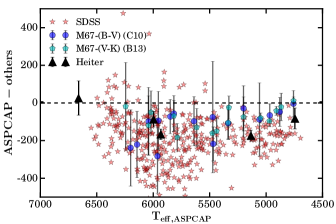
To test the temperature scale further, we calculated photometric temperatures for stars observed by APOGEE in the open cluster M67, which has a well-known solar metallicity, [Fe/H]=$-$0.01 (Jacobson et al., 2011), and reddening, E($B-V$)=0.04 mag (Taylor, 2007), as well as accurate optical $B$ and $V$ band photometry (Sandquist, 2004). To investigate the effect of different color-$T_{\rm eff}$ relations we used Casagrande et al. (2010) to convert $B-V$ colors and Boyajian et al. (2013) to convert $V-K$ colors to temperatures. The uncertainties in the $T_{\rm eff}$ from photometric errors are $<$ 80K. These comparisons are also included in Fig. 1.We also compared the ASPCAP temperatures to the temperatures for five Gaia benchmark stars (Heiter et al., 2015), which are based on interferometric radii and parallax measurements. The random uncertainties in these measurements are $<\,$2%. Figure 1 also shows that the photometric M67 temperatures and Gaia benchmark star temperatures agree well with the SDSS temperature scale, particularly below 6250 K. This agrees with the conclusion of Pinsonneault et al. (2012) that there was good agreement among photometric scales for stars in this temperature range. Therefore, our preferred temperature scale for the Kepler field stars is the SDSS griz temperature scale. For the spectroscopic temperature scale, we include a systematic uncertainty component in the seismically determined stellar parameters to account the systematic offset with respect to the photometric scale. This is done by varying the ASPCAP temperature scales by $\pm 100$ K and quantifying the impact in the final estimated stellar parameters ($g$, $\langle\rho\rangle$, $R$, $M$, and $\tau$). Details are given in Sect. 4.3.3.

At temperatures greater than 6250 K, there are causes for concern for both temperature scales. The near-infrared H-band spectra of hotter stars have fewer absorption features, decreasing their sensitivity to temperature (Holtzman et al 2017 in prep.). Pinsonneault et al. (2012) noted discrepancies among the photometric and spectroscopic measurements when they compared with their SDSS-color based temperatures in this temperature range. Possible reasons include: (1) rapid rotation producing non-isothermal surface temperatures, which violates an assumption of the infrared flux method or, (2) a lack of calibrators for color-$T_{\rm eff}$ relations at these hotter temperatures. Currently ongoing efforts to carefully measure and cross-validate interferometric angular diameters with the CHARA array for a range of spectral types (Karovicova et al., in prep.) as well as planned detailed investigation of individual hot G-stars will contribute to understanding this discrepancy.

2.1.4 Adopted Metallicities

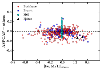
The metallicities ${\rm[M/H]}$ we use throughout this work are the ASPCAP metallicities corresponding to DR13. Formal uncertainties returned by ASPCAP have a median value of 0.025 dex with a very small, 0.004 dex, dispersion. These estimates of uncertainty are based on the small measurement scatter in members of star clusters. Figure 2 shows the comparison of ASPCAP ${\rm[M/H]}$ values with results from optical spectroscopy including ${\rm[Fe/H]}$ measurements for 71 stars in common with the Bruntt et al. (2012) sample and ${\rm[M/H]}$ for 400 stars in common with Buchhave & Latham (2015). The overall agreement is very good in both cases. The median and median absolute deviation of the ${\rm[M/H]}$ difference between ASPCAP and Bruntt et al. (2012) are $-0.019$ dex and 0.052 dex respectively. With respect to Buchhave & Latham (2015) these values are $-0.028$ and 0.046 dex respectively. The figure also shows ASPCAP results for the calibration cluster M67, for which we adopt the mean cluster value ${\rm[Fe/H]}=-0.01\pm 0.05$ dex reported by Jacobson et al. (2011) as our fiducial value. Only stars in the range $\log{g}=3.3$-$4.5$ dex appropriate for our sample are shown. The ASPCAP dispersion for stars in this gravity range is 0.08 dex. Finally, two Gaia benchmark subgiants from Heiter et al. (2015) are also shown.

Based on these comparisons, we do not find significant offsets in the ASPCAP ${\rm[M/H]}$ scale, but typically the dispersion is larger than the formal uncertainties returned by ASPCAP, which highlights the possibility that the true uncertainty is underestimated. In lightof the dispersion that we observe in external measurements of subgiant stars relative to APOGEE, we add a 0.1 dex uncertainty in quadrature to the ASPCAP formal uncertainty, and adopt these as our final ${\rm[M/H]}$ uncertainties for the catalog. Note that in constructing the catalog, we use the same ${\rm[M/H]}$ values in combination with both temperature scales. This is formally inconsistent and might be a systematic source of uncertainty. But, as shown in this section and particularly with the comparison against Buchhave & Latham (2015) results, ASPCAP ${\rm[M/H]}$ determinations are robust so combining them with either temperature scale is a safe procedure.

Figure 2: Differences between ASPCAP metallicities and results from optical spectroscopy Buchhave & Latham (2015) and Bruntt et al. (2012). For M67, our fiducial value is the mean cluster value [Fe/H]=$-$0.01 from (Jacobson et al., 2011).

2.2 Input asteroseismic data

Stars in the APOKASC sample have been observed by Kepler, in cadence of 58.5 s. The sample includes 284 stars observed for up to 40 days, 31 stars between 40 and 100 days, 57 between 100 and 900 days and 55 stars between 900 and 1055 days. Data were downloaded from the KASOC database and corrected using the method presented in Handberg & Lund (2014). This method computes two median-filtered versions of the time series with different filter window widths. A weighted combination is made of the two based on their relative differences to one another — thereby both short and long-term instrumental and transient features are corrected. We refer to Handberg & Lund (2014) for further details on the operations of the filter.

The duration of the timeseries and the brightness of the star are important quantities in determining the quality of the seismic data. The amplitude of solar-like oscillations, however, depends strongly on stellar parameters such as the luminosity $L$, mass $M$, and $T_{\rm eff}$. Huber et al. (2011) has found that oscillation amplitudes in the Kepler photometric band $K_{P}$ behave as $A_{K_{P}}\propto L^{0.838}M^{-1.32}T_{\rm eff}^{-1.8}$ or, using Eq. 1 (Sect. 3, below), as $A_{K_{P}}\propto\nu_{\rm max}^{-1}R^{-0.324}M^{-0.3}T_{\rm eff}^{1.552}$. In the short cadence Kepler sample $\nu_{\rm max}$ varies by more than one order of magnitude while the other quantities in the relation above either vary by much smaller fractions (e.g. $T_{\rm eff}$) or induce milder dependences (e.g. $R$). It is also known that stellar activity may lead to smaller oscillation amplitudes (Chaplin et al., 2011b; García et al., 2010; Kiefer et al., 2017).

A measure of the quality of the seismic detection is given by the height-to-background ratio (HBR), defined as the peak power excess divided by the total power coming from granulation and shot noise at $\nu_{\rm max}$ (see e.g. Mosser et al. 2012). HBR higher than 1 indicates a secure detection. We include HBR as part of the APOKASC catalog presented in this work.

Global seismic parameters $\Delta\nu$ and $\nu_{\rm max}$ were extracted using five independent automated seismic pipelines. This gives us the possibility to of identifying potential issues that might cause systematic offsets in the determination of global seismic parameters or in the determination of uncertainties that could go unnoticed if only one seismic set of results were available. Moreover, this allows have a quantitative estimate of uncertainties linked to the methods used in the seismic pipelines. The procedures employed by each of them are described below.

A2Z: $\Delta\nu$ is obtained by computing the power spectrum of the power spectrum (PS2). The background is fit with a photon noise component and two Harvey-like granulation models (Harvey, 1985) with a slope fixed to 4. A Gaussian function is used to fit the envelope of the p-mode region in a smoothed power spectrum (Mathur et al., 2010). The uncertainties in $\Delta\nu$ and $\nu_{\rm max}$ were computed with the weighted centroids method and are known to be quite conservative. The A2Z pipeline was applied to the KADACS data (García et al., 2011), allowing us to compare the results from different calibrated data.

COR: $\Delta\nu$ is measured with the autocorrelation of the oscillation signal. In practice, this autocorrelation signal is delivered by the power spectrum of the filtered power spectrum of the signal (Mosser & Appourchaux, 2009). The properties of the filter make use of the seismic scaling relations, in order to optimize the seismic signature. A more precise value of the large separation is then obtained using the second-order asymptotic expansion (Mosser et al., 2013). The resulting uncertainty in $\Delta\nu$ is often better than 0.1 %. $\nu_{\rm max}$ and the background parameters are provided by a local analysis of the excess power. The uncertainty in $\nu_{\rm max}$ is a fraction of $\Delta\nu$, typically of about $\Delta\nu/5$.

FITTER: Determination of $\nu_{\rm max}$ is done by performing a Bayesian background fit following Davies & Miglio (2016a). This approach fits a 2 component Harvey model in addition to a Gaussian p-mode hump, all modified by the sinc squared apodization function. A white noise background is added to this. To determine $\Delta\nu$ a squared Gaussian plus a flat background is fitted to a narrow region in the critically sampled power spectrum of the power spectrum (PS2) around half the initial estimate of the large frequency spacing. Estimated values and uncertainties for $\nu_{\rm max}$ and $\Delta\nu$ are determined as the median and the standard deviation of the posterior probability distributions for the central frequencies of the Gaussian components in both methods.

OCT: The background model includes a 2-component Harvey model and a white noise component. After background subtraction, the spectrum is heavily smoothed and a $\nu_{\rm max}$ is obtained from a Gaussian fit to the residual power spectrum. $\Delta\nu$ is determined from a weighted average of the $\Delta\nu/2$ and $\Delta\nu/4$ features extracted from the PS2. The uncertainty is determined as the standard deviation of grouped data following Eq. 6 in Hekker et al. (2010), where more detailes can be found.

SYD: Data are analyzed using the methods described in Huber et al. (2009), using on average a frequency range between 100-7500 $\mu\hbox{Hz}$. The background is modeled using a two component Harvey model with the white noise component fixed to the mean value measured between 7300-7500 $\mu\hbox{Hz}$. Uncertainties on $\Delta\nu$ and $\nu_{\rm max}$ were calculated using Monte-Carlo simulations as described in Huber et al. (2011). The median uncertainties in the sample are  2% in $\Delta\nu$ and  5% in $\nu_{\rm max}$ for stars with less than 100 days of data, and  0.1% and  0.7% for stars observed for the entire mission.

Figure 3: Distribution of errors for global seismic quantities $\nu_{\rm max}$ (left panel) and $\Delta\nu$ (right panel). Vertical dashed, dotted-dashed and solid lines are the median values of the systematic, statistical and total error distributions.

Note that uncertainties returned by each pipeline are formal, in the sense that they do not take into account systematic differences in e.g. the definition of $\Delta\nu$ and $\nu_{\rm max}$. For this reason, results from all pipelines have been used to assess the systematic component contributing to the total uncertainties of the global seismic parameters (for early work on comparisons among seismic pipelines see e.g Verner et al. 2011; Hekker et al. 2011).

For the central values for $\nu_{\rm max}$ and $\Delta\nu$ we adopt results from the SYD pipeline. This choice is made because SYD yields the smallest average deviation from the median values for the sample as a whole and they are available for the complete sample. In addition, it is consistent with that in C14, where the asteroseismic fundamental properties of stars were presented after the initial 10 months of Kepler observations. We define here the formal error given by the SYD pipeline as the statistical uncertainty for each quantity.

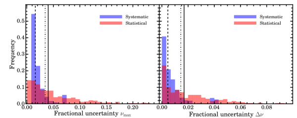
In order to estimate systematic uncertainties we proceed as follows. For $\nu_{\rm max}$ and $\Delta\nu$ separately, we compute $\delta Q_{ij}=(Q_{i,j}-Q_{{\rm SYD},j})/Q_{{\rm SYD},j}$, where $Q$ is either $\nu_{\rm max}$ or $\Delta\nu$, $j$ runs through all stars in the sample and $i$ over all the pipelines other than SYD. We define clear outliers as measurements $Q_{i,j}$ for which $|\delta Q_{ij}|>0.2$. There are 71 individual measurement, i.e. combinations of $(i,j)$ from all non-SYD pipelines that fall in this condition for either $\nu_{\rm max}$ or $\Delta\nu$. This is equivalent to about 4% of the measurements for all non-SYD pipelines. These outliers are removed from the estimate of systematic uncertainties. The resulting distributions of $\{\delta Q_{ij}\}$ are characterized by mean values of 0.1% and 0.02% for $\nu_{\rm max}$ and $\Delta\nu$, respectively, and standard deviations of $\sigma_{\rm sys}(\nu_{\rm max})=3.3\%$ and $\sigma_{\rm sys}(\Delta\nu)=2\%$. The mean values indicate that there are no strong systematic deviations among pipelines. Then, we define thresholds of 7% and 4%, equal to twice the values of $\sigma_{\rm sys}(\nu_{\rm max})$ and $\sigma_{\rm sys}(\Delta\nu)$. For each star, we now compute the median of a given seismic quantity and remove results discrepant from this median by more than the threshold defined above. The process is iterated until no outliers are found or only results from two pipelines remain. The 1 $\sigma$ systematic uncertainty for each seismic quantity and star is then defined as the standard deviation of the remaining values. SYD results are always kept because they constitute the central seismic values used in this work. If only the SYD result is available, then a systematic uncertainty equal to the threshold value is assigned.

The final distributions of statistical (SYD) and systematic uncertainties are shown for $\nu_{\rm max}$ and $\Delta\nu$ in the two panels of Fig. 3. For both quantities statistical uncertainties have much more extended distributions, i.e. they dominate the total error for the majority of the sample. In the case of the systematic distributions, two small bumps are seen at 7% and 4% for $\nu_{\rm max}$ and $\Delta\nu$ respectively that correspond to stars with results just from SYD. For each star, the total error is computed by adding in quadrature the systematic and statistical uncertainties. Vertical lines show the median values of systematic, statistical and total errors in increasing order. The latter are 4% for $\nu_{\rm max}$ and 1.7% for $\Delta\nu$.

sec:systgbm

3 Grid-based modeling

Stellar mass and radius can be estimated from the global seismic parameters $\nu_{\rm max}$ and $\Delta\nu$, and $T_{\rm eff}$. If $g$ is the stellar surface gravity, $\langle\rho\rangle$ the mean density, $M$ the mass, and $R$ the radius, then the scaling relations (Ulrich, 1986; Brown, 1991; Kjeldsen & Bedding, 1995)

$$\frac{\nu_{\rm max}}{\nu_{\rm max,\odot}} \simeq\left(\frac{g}{\rm g_{\odot}}\right)\left(\frac{T_{\rm eff}}{\rm T_{eff,\odot}}\right)^{-1/2}$$ (1)

$$\frac{\Delta\nu}{\Delta\nu_{\odot}} \simeq\left(\frac{\langle\rho\rangle}{\langle\rho_{\odot}\rangle}\right)^{1/2}$$ (2)

can be readily inverted such that stellar mass and radius are approximately given by

$$\frac{M}{{\rm M_{\odot}}} \simeq\left(\frac{\nu_{\rm max}}{\nu_{\rm max,\odot}}\right)^{3}\left(\frac{\Delta\nu}{\Delta\nu_{\odot}}\right)^{-4}\left(\frac{T_{\rm eff}}{\rm T_{eff,\odot}}\right)^{3/2}$$ (3)

$$\frac{R}{{\rm R_{\odot}}} \simeq\left(\frac{\nu_{\rm max}}{\nu_{\rm max,\odot}}\right)\left(\frac{\Delta\nu}{\Delta\nu_{\odot}}\right)^{-2}\left(\frac{T_{\rm eff}}{\rm T_{eff,\odot}}\right)^{1/2}.$$ (4)

Direct determination of $M$ and $R$ from the equations above can be qualitatively improved by constructing grids of stellar evolutionary tracks that include $\nu_{\rm max}$ and $\Delta\nu$. A more refined analysis is possible when information about the composition of the star is also available, e.g. by means of ${\rm[M/H]}$. Then, a given set of observables is compared against a large set of stellar models from which best fitting values and uncertainties or even full statistical distributions for the stellar quantities of interest can be determined. This so-called grid-based modeling (GBM) allows the estimation of other quantities beyond mass and radius, most importantly stellar age $\tau$.

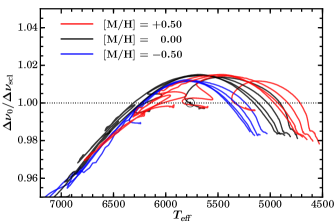
Scaling relations (Eqs. 1-2) applied to dwarfs and subgiants are accurate to within a few percent (Stello et al., 2009a; Huber et al., 2012; Silva Aguirre et al., 2012; White et al., 2013; Coelho et al., 2015; Huber et al., 2017). The first relation is qualitatively understood by theory of stochastically excited oscillations, but its accuracy still defies a definite understanding (Belkacem et al., 2011). On the other hand, the relation for $\Delta\nu$ can be tested by stellar models, at least up to the point allowed by adiabatic oscillation frequencies or the poor modeling of surface effects. In fact, Eq. 2 can be dropped altogether in GBM if, for each stellar model in the grid, $\Delta\nu$ is computed from an appropriate fit to the model frequencies of radial ($\ell=0$) modes. White et al. (2011) found that for main sequence and subgiant stars $\Delta\nu$ derived from model frequencies deviate from Eq. 2 by a few percent, with clear trends depending on the stellar $T_{\rm eff}$. In the remainder of this work we denote by $\Delta\nu_{0}$ the large frequency separation determined in stellar models by using frequencies from $\ell=0$ modes and by $\Delta\nu_{\rm scl}$ the large frequency separation obtained when Eq. 2 is used to compute it in stellar models. Figure 4 shows the relative difference between $\Delta\nu_{0}$ and $\Delta\nu_{\rm scl}$ as a function of $T_{\rm eff}$ for representative evolutionary tracks based on a calibration that reproduces the global seismic solar properties. The mass range of the tracks shown is between 1 and 1.6 M_⊙ and tracks cover all evolutionary phases of interest for our catalog, from ZAMS up to evolved subgiant phase (defined here for illustration purposes as $\log{g}=3.2$). As shown in Fig. 1, $T_{\rm eff}$ in our APOKASC sample range from $\sim 6500$ down to $\sim 4700$ K. Then, from Fig. 4 we see that $\Delta\nu_{0}$ departures from the pure $\Delta\nu_{\rm scl}$ scaling relation can vary between approximately $-3$% and 2% depending on the stellar mass, $T_{\rm eff}$ and ${\rm[M/H]}$. In later sections we discuss in detail the impact of these departures in the determination of fundamental stellar parameters.

Figure 4: Ratio between $\Delta\nu_{0}$ and $\Delta\nu_{\rm scl}$ for stellar models with 1, 1.2, 1.4, and 1.6 M_⊙ (from right to left at the low $T_{\rm eff}$ end) and ${\rm[M/H]}=-0.5,0.0,+0.5$ (blue, black and red respectively). At low $T_{\rm eff}$ tracks are truncated at $\log{g}=3.2$ because all APOKASC sample has higher $\log{g}$.

For this catalog, determination of stellar parameters is based upon GBM. By construction, unlike the plain use of scaling relations, GBM introduces dependencies on stellar models and also on the statistical approach employed to characterize stellar quantities of interest. In a similar manner as done with asteroseismic pipelines, we use a number of GBM pipelines that employ different stellar models and/or statistical methods. In this way, we aim not only at determining stellar parameters but also at obtaining a sensible quantification of the systematic uncertainties involved. In total, we have employed seven different GBM pipelines but some of them have been run in more than one mode, i.e. with different sets of stellar models or assumptions regarding calculation of $\Delta\nu$, leading to a grand total of twelve different sets of GBM results.

Here we include a summary of the characteristics of the different GBM calculations, sorted by pipelines. A list of the combinations of grids of stellar models, GBM pipelines, and choice of $\Delta\nu_{0}$ or $\Delta\nu_{\rm scl}$ used in this work is given for quick reference in Table 1. A description of the physical inputs adopted in each of the grids of stellar models is presented in Appendix A. Additional details about the numerical methods of different pipelines are given in the respective references.

BASTA: For this work, the BAyesian STellar Algorithm (Silva Aguirre et al., 2015) uses stellar models computed with GARSTEC (Weiss & Schlattl, 2008). The mass and ${\rm[Fe/H]}$ ranges covered by the grid are M/${\rm M_{\odot}}=\left\{0.7\,,1.80\right\}$ with $\Delta M=0.01\,{\rm M_{\odot}}$ and ${\rm[Fe/H]}=\left\{-0.65\,,+0.50\right\}$ dex with $\Delta{\rm[Fe/H]}$ = 0.05 dex respectively. Determination of stellar parameters is performed with an adapted version of the Bayesian approach described in Serenelli et al. (2013). BASTA has been run both with $\Delta\nu_{0}$ and $\Delta\nu_{\rm scl}$, that we identify as BAS/G-$\Delta\nu_{0}$ and BAS/G-$\Delta\nu_{\rm scl}$. For each quantity, its central value and $\pm 1\sigma$ limits correspond to the median and the $\pm 34.1\%$ limits around the median respectively.

BeSPP: The Bellaterra Stellar Parameters Pipeline uses stellar models computed with GARSTEC but with some differences with respect to those used in BASTA. The grid covers the range M/${\rm M_{\odot}}$=$\left\{0.6\,,3.0\right\}$ with a step $\Delta{\rm M}/{\rm M_{\odot}}=0.02$ and [Fe/H]=$\left\{-3.0\,,+0.6\right\}$ dex with $\Delta{\rm[Fe/H]}=0.1$ dex for ${\rm[Fe/H]}$ between $-$3.0 and 0.0 dex and $\Delta{\rm[Fe/H]}=0.05$ dex for ${\rm[Fe/H]}>0.0$ dex. The determination of stellar parameters is done by means of a Bayesian approach based on the method described in Serenelli et al. (2013), extended to include asteroseismic inputs. BeSPP has been run both with $\Delta\nu_{0}$ and $\Delta\nu_{\rm scl}$: BeS/G-$\Delta\nu_{0}$ and BeS/G-$\Delta\nu_{\rm scl}$. For each quantity, its central value and $\pm 1\sigma$ limits correspond to the median and the $\pm 34.1\%$ limits around the median respectively.

GOE: Two grids of stellar models have been used, one computed with CESTAM2k (Marques et al., 2013) and the other one with MESA (Paxton et al., 2013). Both grids span the mass range M/${\rm M_{\odot}}$=$\left\{0.6\,,2.0\right\}$ with $\Delta M=0.02\,{\rm M_{\odot}}$. The metallicity range Z$=\left\{0.003\,,0.040\right\}$ with a 0.003 step, which is roughly equivalent to ${\rm[Fe/H]}=\left\{-1.3\,,+0.40\right\}$ dex. The CESTAM2k grid has been run with $\Delta\nu_{0}$ and $\Delta\nu_{\rm scl}$ and the MESA grid just with $\Delta\nu_{\rm scl}$: GOE/C-$\Delta\nu_{0}$, GOE/C-$\Delta\nu_{\rm scl}$, and GOE/M-$\Delta\nu_{\rm scl}$. The determination of stellar parameters is based on an independent implementation of SEEK (Quirion et al., 2010), but adopting Bayesian priors only to account for the inhomogeneity sampling of the grids of stellar models (Hekker & Ball, 2014). For each quantity, its central value and $\pm 1\sigma$ limits correspond to the median and the $\pm 34.1\%$ limits around the median respectively.

MPS: This pipeline is based on an independent implementation of the likelihood method described in Basu et al. (2010). It is based on a Monte Carlo method in which observed parameters are sampled and, for each realization, the likelihood of all models in the grid is computed. All of this likelihood distributions are then combined to obtain the global likelihood distribution from which stellar parameters and uncertainties are determined (Hekker & Ball, 2014). Stellar models are the canonical models (no overshooting) of BaSTI (Pietrinferni et al., 2004), span the mass and metallicity ranges M/${\rm M_{\odot}}$=$\left\{0.5\,,4.5\right\}$ with $\Delta M=0.05\,{\rm M_{\odot}}$ and Z$=\left\{0.0001\,,0.040\right\}$, and use $\Delta\nu_{\rm scl}$. We identify it as MPS/B-$\Delta\nu_{\rm scl}$.

RADIUS: Stellar models are computed with ASTEC (Christensen-Dalsgaard, 2008). The grid covers M/${\rm M_{\odot}}$=$\left\{0.5\,,4.0\right\}$ with a step $\Delta{\rm M}/{\rm M_{\odot}}=0.01$ and [Fe/H]=$\left\{-1.27\,,+0.47\right\}$ dex with $\Delta{\rm[Fe/H]}=0.1$ dex and employs $\Delta\nu_{\rm scl}$. We name it RAD/A-$\Delta\nu_{\rm scl}$. Central values of stellar parameters are determined from the best fitting model and the 1$\sigma$ uncertainties are estimated by considering the full range of values of a given parameter spanned by the models that are within 3 $\sigma$ of all the input parameters, and assuming it represents a $\pm 3\sigma$ range of the output parameters (Stello et al., 2009b).

SFP: Seismic Fundamental Parameters. Stellar models in SFP are the BaSTI canonical models (Pietrinferni et al., 2004). The grid covers the range M/${\rm M_{\odot}}$=$\left\{0.7\,,4.5\right\}$ and Z$=\left\{0.001\,,0.040\right\}$ and it has been interpolated to offer a denser representation of the parameter space so that $\Delta{\rm M}/{\rm M_{\odot}}=0.02$ and $\Delta\rm{Z}=0.001$. In this implementation, SFP/B-$\Delta\nu_{\rm scl}$, $\Delta\nu_{\rm scl}$ is used, and the determination of stellar parameters is done with a Bayesian method, as described in Kallinger et al. (2010) and Kallinger et al. (2012). The central value quoted for a given stellar quantity is the most probable value in the distribution and the $\pm 1\sigma$ values correspond to the limits containing $\pm 34.1\%$ of the probability distribution around the most probable value.

YB: The Yale-Birmingham pipeline (Basu et al., 2010; Gai et al., 2011) has been run with two different grids of stellar models. One grid has been computed with YREC2 and covers M/${\rm M_{\odot}}$=$\left\{0.8\,,3.0\right\}$ with a step $\Delta{\rm M}/{\rm M_{\odot}}=0.02$ and [Fe/H]=$\left\{-0.6\,,+0.6\right\}$ dex with $\Delta{\rm[Fe/H]}=0.05$ dex. The other one is formed by the canonical models from BaSTI (Pietrinferni et al., 2004) (see MPS above). Both grids use $\Delta\nu_{\rm scl}$ and we identify them as YB/YR-$\Delta\nu_{\rm scl}$ and YB/B-$\Delta\nu_{\rm scl}$. Stellar parameters are determined through a Monte Carlo approach, where input data is used to generate large Gaussian samples of input parameters. The stellar parameters of the model with highest likelihood is assigned to each realization of the sample. These models are then used to build the probability distribution. For each quantity, its central value and $\pm 1\sigma$ limits correspond to the median and the $\pm 34.1\%$ limits around the median respectively.

Table 1: Summary of GBM

GBM	Stellar code	Mode	Short name	GBM	Stellar code	Mode	Short name
BASTA	GARSTEC	$\Delta\nu_{\rm scl}$	BAS/G-$\Delta\nu_{\rm scl}$	GOE	MESA	$\Delta\nu_{\rm scl}$	GOE/M-$\Delta\nu_{\rm scl}$
BASTA	GARSTEC	$\Delta\nu_{0}$	BAS/G-$\Delta\nu_{0}$	MPS	BASTI	$\Delta\nu_{\rm scl}$	MPS/B-$\Delta\nu_{\rm scl}$
BeSPP	GARSTEC	$\Delta\nu_{\rm scl}$	BeS/G-$\Delta\nu_{\rm scl}$	RADIUS	ASTEC	$\Delta\nu_{\rm scl}$	RAD/A-$\Delta\nu_{\rm scl}$
BeSPP	GARSTEC	$\Delta\nu_{0}$	BeS/G-$\Delta\nu_{0}$	SFP	BASTI	$\Delta\nu_{\rm scl}$	SFP/B-$\Delta\nu_{\rm scl}$
GOE	CESTAM2k	$\Delta\nu_{\rm scl}$	GOE/C-$\Delta\nu_{\rm scl}$	YB	YREC2	$\Delta\nu_{\rm scl}$	YB/YR-$\Delta\nu_{\rm scl}$
GOE	CESTAM2k	$\Delta\nu_{0}$	GOE/C-$\Delta\nu_{0}$	YB	BASTI	$\Delta\nu_{\rm scl}$	YB/B-$\Delta\nu_{\rm scl}$

Note. — $\Delta\nu_{\rm scl}$ stands for $\Delta\nu$ as obtained directly from Eq. (2) and $\Delta\nu_{0}$ for $\Delta\nu$ obtained from the slope of a linear fit to radial model frequencies (Sect. 3).

4 Determination of stellar parameters and uncertainties

4.1 Choice of central values

The combination of spectroscopic and asteroseismic data is used in this work to produce a catalog that includes determinations of the following quantities: $g$, $\langle\rho\rangle$, $M$, $R$, and $\tau$. The central values in the catalog correspond to the determination of these quantities obtained with the combination BeSPP,GARSTEC,$\Delta\nu_{0}$, or BeS/G-$\Delta\nu_{0}$ for short. This choice is based on the following reasons.

The grid of stellar models used in BeSPP is the only one in this work that includes microscopic diffusion (see Appendix A for details on the implementation). This is a relevant physical process for solar-like stars. In the particular case of the Sun, it is necessary to include it in order to obtain a good agreement with helioseismic measurements (see Bahcall et al. 1995; Christensen-Dalsgaard et al. 1996 among many others). Additional evidence of microscopic diffusion can be found in high precision spectroscopic work on clusters that show depletion of metals of up to 0.2 dex in the very metal poor clusters NGC6397 and M30 (Nordlander et al., 2012; Gruyters et al., 2016) and a more subtle depletion, below a 0.1 dex level, in the higher metallicity clusters NGC 6752 and M67 (Gruyters et al., 2014; Önehag et al., 2014).

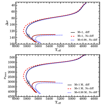
An additional reason is that the solar calibrations performed to fix the mixing length parameter $\alpha_{c}$ are typically done including microscopic diffusion. But then, when the grids are computed neglecting this process, a mismatch is produced between the calibrated $T_{\rm eff}$ scale set by the solar calibrated $\alpha_{c}$ and the actual $T_{\rm eff}$ scale in the grid. In practice, this implies that grids computed in this way do not contain a model that reproduces the basic solar properties, i.e. solar radius and luminosity at the present-day solar age. To illustrate this, Figure 5 shows, in the $T_{\rm eff}-\Delta\nu$ and $T_{\rm eff}-\nu_{\rm max}$ planes, the evolutionary track of a 1 M_⊙ solar calibrated track including diffusion (solid black line) and the corresponding track using the same calibrated mixing length $\alpha_{c}$ but without diffusion (dashed red line). It is apparent from these figures that solar seismic properties cannot be reproduced by the evolutionary model that does not include diffusion. The mismatch corresponds, approximately, to a 0.02 M_⊙ difference, as seen by the overlap between the 0.98 M_⊙ evolutionary track without microscopic diffusion (blue dotted line) and the solar calibrated track. This might not seem as a large effect, but as we discuss in later sections, this is a sizeable number compared to typical mass uncertainties determined from asteroseismic data. The mismatch between tracks with or without diffusion depends on the evolutionary stage; it builds up starting from the ZAMS, it is maximum at the turn off, and it almost completely vanishes as stars evolve off the main sequence and the convective envelope deepens, restoring the initial surface composition.

Figure 5: Comparison of 1 ${\rm M_{\odot}}$ evolutionary tracks using the same solar calibrated mixing length and same initial composition, with and without microscopic diffusion. The top (bottom) panel shows $\Delta\nu$ ($\nu_{\rm max}$) as a function of $T_{\rm eff}$. For given observables around the turn-off, the difference in mass is about 0.02 ${\rm M_{\odot}}$, as shown by the 0.98 ${\rm M_{\odot}}$ track without diffusion. Circle denotes the position of the Sun.

The final reason for using BeS/G-$\Delta\nu_{0}$ results as the reference values in the catalog relates to the calculation of $\Delta\nu_{0}$. There are three sets of results based on GBMs that rely upon $\Delta\nu_{0}$, BAS/G-$\Delta\nu_{0}$, BeS/G-$\Delta\nu_{0}$, and GOE/C-$\Delta\nu_{0}$. The advantage of relying on $\Delta\nu_{0}$ is that it captures deviations from the pure scaling $\Delta\nu_{\rm scl}$ due to detailed structure of stellar models (see e.g. Belkacem et al. 2013). But, its determination from theoretical frequencies is affected by poor modeling of stellar atmospheres and the neglect of non-adiabatic effects in the outermost layers of stars (Rosenthal et al., 1999). In the BeS/G-$\Delta\nu_{0}$ grid for example, the solar model gives $\Delta\nu_{0}=136.3\,\mu$Hz, about 1% larger than the reference $\Delta\nu_{\odot}=135.1\pm 0.1\,\mu$Hz determined from the SYD seismic pipeline. This difference implies that grids relying on $\Delta\nu_{0}$ will not be able to reproduce a solar model unless they are rescaled so that $\Delta\nu_{0}$ for the solar model matched $\Delta\nu_{\odot}$. Such correction is applied in BeS/G-$\Delta\nu_{0}$  by computing a calibration factor $f_{\Delta\nu}=\Delta\nu_{\odot}/\Delta\nu_{0,\rm SM}$ (here SM means solar model) and rescaling $\Delta\nu_{0}$ in the whole grid according to it. Other grids based on $\Delta\nu_{0}$ do not correct for this effect and therefore do not reproduce solar properties when fed with solar seismic quantities. Applying this correction factor to the whole grid of stellar models carries the implicit assumption that the surface effect produces a fractional variation in $\Delta\nu$ that is constant for all stars, analogous to using a fixed $\alpha_{c}$ based on a solar calibration. Work is ongoing in developing surface effect corrections (e.g. Sonoi et al. 2015; Ball & Gizon 2014) and more sophisticated model atmospheres to have more realistic calculations of frequencies and, in the context of the present work, corrections to $\Delta\nu_{0}$ that do not rely on solar scaling (Ball et al., 2016; Trampedach et al., 2017).

Figure 6: Statistical errors for all stars and all pipelines (see Table 1 for a full list of pipelines).

The underlying differences between BeS/G-$\Delta\nu_{0}$ used to provide the central values in the catalog and other GBMs are in fact a positive aspect in our work because they allow a more robust determination of systematic uncertainties, as discussed later in Section 4.3.1.

4.2 Statistical uncertainties

The adopted formal uncertainties from ASPCAP are 69 K for $T_{\rm eff}$ and, typically, 0.10 dex for ${\rm[M/H]}$ (Sect. 2.1). In the SDSS scale, $T_{\rm eff}$ errors are characterized by a mean of 67 K, very similar to the ASPCAP formal error, with a dispersion of 25 K. Metallicities are those from ASPCAP so their uncertainties are treated in the way described above.

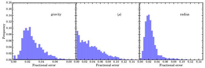
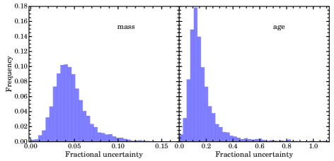
Each GBM pipeline returns central values and uncertainties for each of the stellar parameters included in the catalog, i.e. $M$, $R$, $\langle\rho\rangle$, $g$ and $\tau$. The uncertainty returned by each pipeline is the statistical uncertainty associated with each parameter, a measure of the precision with which stellar parameters can be determined from the available spectroscopic and asteroseismic data. For each stellar parameter, the distribution of statistical uncertainties from all twelve GBM sets is shown in Fig. 6. This figure shows results obtained using the ASPCAP spectroscopic parameters but, due to the similarity in $T_{\rm eff}$ statistical uncertainties between the ASPCAP and the SDSS temperature scales, results and the discussion that follows are very similar for both scales.

Figure 7: Relation between mass and age statistical uncertainties. Color coded is the central hydrogen mass fraction $X_{c}$. Stars with $X_{\rm c}<0.02$ are shown as black symbols. Dashed line represents a 3:1 relation between age and mass uncertainties.

Interpreting the distribution of statistical uncertainties for $g$ and $\langle\rho\rangle$ is straight forward from the scaling relations. For $g$, the dominant error source comes from the linear dependence of $g$ with $\nu_{\rm max}$. The additional dependence on $\sqrt{T_{\rm eff}}$ is small because $\delta T_{\rm eff}/T_{\rm eff}$ ranges between 1 and 1.5% for the whole sample, so this propagates at most as a 0.7% ($<0.01$ dex) uncertainty into $g$. For $\langle\rho\rangle$, the dominant uncertainty source is $\Delta\nu$, augmented by the corresponding factor of 2. To first order, there is no explicit dependence of $\langle\rho\rangle$ on other quantities than $\Delta\nu$, and given that the $\Delta\nu$ uncertainty distributions does not peak, neither does the distribution of $\langle\rho\rangle$ statistical uncertainties.

For radius, this discussion is more interesting and it is a good example of the advantages of using GBM to determine stellar parameters instead of relying simply on the scaling relations. Let us consider the median fractional uncertainties of $\nu_{\rm max}$ and $\Delta\nu$ shown in Fig. 3 as an example. These are 4% and 1.7% respectively, and assume a 1.3% fractional uncertainty for $T_{\rm eff}$ (corresponding to a typical $T_{\rm eff}=5400$ K value). Using Eq. 4 to propagate these errors we obtain an estimate of the median fractional uncertainty of $\delta R/R\approx 5\%$. However, the distribution in Fig. 6 shows a distribution that peaks around 2% and, in fact, 89% of the GBM results have $\delta R/R<4.5\%$. The reason for this apparent discrepancy is that $\nu_{\rm max}$ and $\Delta\nu$ are not independent quantities in stars, as they both depend on the same intrinsic quantities. Stellar evolution models used in GBM incorporate by construction their correlation. Based on stellar models, Stello et al. (2009a) have found the simple relation $\Delta\nu\propto\nu_{\rm max}^{0.77}$ between these quantities. Using this relation, we can go back to Eq. 4 and, because typically $\nu_{\rm max}$ has a larger fractional uncertainty than $\Delta\nu$, replace $\Delta\nu$ by its dependence on $\nu_{\rm max}$ to find an approximate relation $R\propto(T_{\rm eff}/\nu_{\rm max})^{1/2}$. Now, using the median uncertainty for $\nu_{\rm max}$ and 1.3% for $T_{\rm eff}$ as before we obtain $\delta R/R\approx 2.2\%$, well in agreement with the distribution seen in Fig. 6. Linear propagation of errors from Eq. 4 without accounting for physical correlation between $\nu_{\rm max}$ and $\Delta\nu$ leads to an overestimation of uncertainties in the inferred stellar parameters. Gai et al. (2011) already discussed that GBM leads to smaller errors than direct application of Eq. 4, but the simple explanation related to the $\nu_{\rm max}-\Delta\nu$ relation being imprinted in stellar models was not discussed in that work.

There is an analogous discussion for the statistical uncertainty in the determination of stellar masses. Use of scaling relations leads to overestimation of the uncertainty because there is no information on stellar structure and evolution in those relations. Using median uncertainties as above, we derive an expected $\delta M/M\approx 14\%$, more than three times the median value in the distribution of statistical uncertainties shown in Fig. 6. Again, accounting for the correlation between $\nu_{\rm max}$ and $\Delta\nu$ leads to a much smaller value of $\sim 2\%$. Note that in this §estimate the fractional uncertainty of $\Delta\nu$ is assumed to be that of $\nu_{\rm max}$ scaled by the factor 0.77. It is a crude estimate, but good enough to guide interpretation of uncertainties in mass determinations. The uncertainty distribution of masses shown in Fig. 6 shows, however, a maximum around 3.5-4%, larger than the above estimate. This is mostly due to the effect of the metallicity uncertainty, which is not taken into account in scaling relations. In fact, there is a correlation between metallicity and seismic mass determinations such that a 0.1 dex uncertainty in ${\rm[M/H]}$ corresponds to about 2.5-3% uncertainty in mass (Sect. 5.3.1). This uncertainty, combined with the 2% mass uncertainty estimated from seismic quantities and $T_{\rm eff}$ gives a good understanding of the typical statistical mass uncertainty we have found in our GBM results.

The discussion above is simplified, for example in that the role of stellar metallicity is not accounted for, but it shows that using GBM is not only qualitatively better than employing scaling relations because it incorporates knowledge on stellar structure, but in fact leads to more precise estimations of stellar parameters because models naturally incorporate existing correlations between physical quantities. Typically, we can conclude that GBM leads to a precision in mass and radius that is at least a factor of two better than pure scaling relations. Moreover, it is so due to good physical reasons.

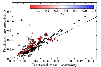
Finally, interpretation of statistical uncertainties of stellar ages depends on the evolutionary state of the star. The total evolutionary lifetime of a star on the main sequence scales approximately with its mass as $\tau_{\rm MS}\propto M^{-\alpha}$, with $\alpha\approx 3-3.5$ for low mass stars (Serenelli & Fukugita, 2007). Therefore, for stars at the end or past the main sequence, it is expected that the age uncertainty is roughly $\alpha$ times the mass uncertainty. Fig. 7 shows the relation between mass and age uncertainties obtained with BeSPP, and color coded according to the central hydrogen abundance, a measure of the evolutionary status of each star. For stars that have depleted hydrogen (black symbols), which in fact comprise most of the sample, the linear relation is clearly visible. For stars that are still on the main sequence, the correlation between mass and age is naturally lost because the stellar mass does not determine its current age. In practice, results shown in Fig. 7 allow to establish, as a rule of thumb, that a lower bound for the fractional age uncertainty is $\delta\tau/\tau\gtrsim 3\cdot\delta M/M$ (see also Davies & Miglio 2016b).

4.3 Systematic uncertainties

4.3.1 GBM peculiarities

The second major source of uncertainties has its origin in the GBM pipelines. Several aspects need to be considered: the stellar evolution tracks, the statistical method to extract stellar parameters, and the calculation of $\Delta\nu$ in evolutionary tracks.

As described in Sect. 3, different pipelines typically employ different grids of stellar models. Stellar evolution theory still has some uncertainty; there is not a unique choice of what different modelers consider is the best physics that should be employed in computation of stellar models. In the realm of low mass stars, different possibilities are available, among others, for nuclear reaction rates, radiative opacities (atomic and molecular), treatment of microscopic diffusion, implementation and amount of overshooting among other physical inputs or processes. Moreover, different numerical implementations of similar physics and numerical aspects of the integration of the equations of stellar structure and evolution can also lead to differences in the computed stellar models. Detailed comparisons of stellar models for dwarf stars using different physics but the same code or different codes but the same underlying physics, have been object of some studies, although of limited scope (Lebreton et al. 2008; Marconi et al. 2008; Stancliffe et al. 2016 among others). Additionally, GBM pipelines can implement differently a given set of stellar tracks (e.g. interpolating stellar tracks to a finer grid) and also employ different statistical approaches to extract stellar parameters and their uncertainties so even using the same underlying grid of stellar models does not imply that different GBM pipelines will lead to the same results.

Figure 8: Fractional differences (except for $\log{g}$, given in dex) in the estimated stellar parameters from different GBM pipelines. Pairs of GBMs used in each column and sense in which differences are computed are listed at the top using the form: Pipeline/Grid-$\Delta\nu$ type (see Sect. 3 and Table 1 for naming convention). The columns are from left to right: (1) Same pipeline but different models, (2) different pipeline but the same models, (3) same pipeline and models but different $\Delta\nu$ type and, (4) same pipeline and model but different $\Delta\nu$ type both scaled to solar. Red solid and blue dashed lines show statistical uncertainties returned by the first and second pipelines respectively, in bins of 60 K.

C14 has considered this problem and performed several comparisons aimed at disentangling the effects of statistical methods and the use of different grids of stellar models. Here, we have also carried out such comparisons based on results from the twelve GBM sets of results available (Table 1). Extensive GBM one-to-one comparisons are presented in Appendix B. In this section, we use a subset of results to illustrate the typical systematic uncertainties arising from four different sources: different evolutionary tracks, different statistical methods to determine stellar parameters, the use of $\Delta\nu_{0}$ or $\Delta\nu_{\rm scl}$, and the solar calibration of $\Delta\nu_{0}$ (Sect. 4.1).

The typical relevance of each uncertainty source is shown, for all stellar parameters, in Figure 8 where each column of plots shows relative differences in the central values of the stellar parameters determined with two different GBM runs that differ from one another in just one aspect. Differences are taken in the sense indicated at the top of each column. In each plot, red solid and blue dashed lines are the statistical uncertainties returned by the first and second pipelines respectively, binned in 60 K intervals. Note that it is not within the scope of this paper to look into detail on the origin of the differences among GBM results, but rather to present typical cases and point out some possible causes for systematic differences.

The first column of plots in Fig. 8 compares results obtained with the YB pipeline but with different evolutionary tracks, YREC2 or BaSTI. For $g$, $\langle\rho\rangle$, $R$, and $M$ a systematic offset is seen between the sets of results. A possible reason for systematic offset could be that $T_{\rm eff}$ scales or even luminosities in the models are somewhat different. A mismatch in the $T_{\rm eff}$ scale is possible even if both sets of tracks are based on a solar calibration of the mixing length parameter, especially if the solar calibration and the evolutionary tracks have been computed with different physical assumptions. This is the case of the BaSTI tracks, that include microscopic diffusion in the solar calibration but do not in the library of stellar models Pietrinferni et al., 2004, which leads to a $T_{\rm eff}$ offset as discussed in Sect. 4.1. Another source of differences might be the choice of the critical ${\rm{}^{14}N(p,\gamma)^{15}O}$ rate, which is about a factor of two smaller in YREC2 than in BaSTI (see Table 7 and 8 in Appendix A for a description of input physics used in the stellar models used in this work). This rate affects the $T_{\rm eff}$ scale of low mass stars (typically $M<1.3{\rm M_{\odot}}$) close to the turn-off, when the CNO-cycle takes over pp-chains as the dominant H-burning process. It also affects the whole main sequence for more massive models and the luminosity of the subgiant branch, where models with a larger rate are less luminous (Magic et al., 2010).

An additional difference is the inclusion (YREC2), or not (BaSTI models used in this work), of overshooting, which will also affect the $T_{\rm eff}$ scale of stellar models that have a convective core during the main sequence. It is also interesting that the systematic offset in stellar mass is not translated into ages, as it would be naively expected. This points towards YREC2 predicting longer main sequence lifetimes than BaSTI, which is consistent (at least for stars with $M\gtrsim 1.2\,{\rm M_{\odot}}$ that have convective cores during the main sequence) with the fact that YREC2 models include convective overshooting whereas the BaSTI models used here do not. It is also possible that, even in the absence of convective cores during the main sequence, BaSTI and YREC2 models do not predict the same evolutionary timescales at equal stellar mass and composition.

Despite all the above differences, it is reassuring that in almost all cases the differences are smaller or comparable to the 1$\sigma$ statistical uncertainties returned by the pipelines. The exception is a small number of stars with $T_{\rm eff}<5400$ K for which $R$ and $M$ have larger fractional differences.

The second column compares results obtained by two sets of GBM results that employ the same underlying set of BaSTI tracks but that are implemented differently. These two GBMs, SFP/B and MPS/B also determine central parameters and uncertainties by different methods as well. Here it is very difficult to single out reasons why results from both GBM pipelines show such dispersions. A clear difference is the mass resolution because SFP/B uses an interpolated grid with a finer mass resolution than the original BaSTI grid. This may play an important role especially when seismic uncertainties are small, which can lead to statistical uncertainties well below the mass resolution of the grid. For all stellar quantities, the dispersion of results seen among pipelines sharing the same evolutionary tracks is comparable to those seen in the first column, showing the same pipeline with different stellar models. Again, we note that systematic differences are almost in all cases not larger than statistical uncertainties returned by the pipelines.

The third column compares results from the BAS/G pipeline where the only difference is the use of $\Delta\nu_{\rm scl}$ or $\Delta\nu_{0}$. This case has also been discussed in the literature, as described in Sect. 3, but with emphasis in the change in $\langle\rho\rangle$, that is most directly affected by the choice of $\Delta\nu$ in the stellar models. Clearly, and as expected, the systematic effects follow the inverted shape of the $\Delta\nu_{0}/\Delta\nu_{\rm scl}$ ratio (Fig. 4) multiplied by 2. This clear trend with $T_{\rm eff}$ is also reflected in $R$ and $M$ estimates, and also in $\log{g}$, which to first order is independent of $\Delta\nu$ according to the scaling relations. Stellar ages are affected as well, but in this case they reflect an almost one-to-one correspondance with the mass variation, so changes are quite small. Note that $\Delta\nu_{\rm scl}$ has been scaled such that the reference solar $\Delta\nu_{\odot}=135.1\mu$Hz is reproduced. On the other hand, the grid using $\Delta\nu_{0}$ has not been calibrated to match $\Delta\nu_{\odot}$.

Column four compares results from BeS/G-$\Delta\nu_{\rm scl}$ and BeS/G-$\Delta\nu_{0}$ and in this case both $\Delta\nu_{\rm scl}$ and $\Delta\nu_{0}$ have been rescaled, as explained in Sect. 4.1, so that a solar model is reproduced properly. The trends seen in the plots of this column are very similar to those in the previous column but with an offset that reflects the rescaling of $\Delta\nu_{0}$ by the factor $f_{\Delta\nu}$ defined in Sect. 4.1. It is important to point out that, despite the $f_{\Delta\nu}$ correction (or calibration) factor, the differences between BeS/G-$\Delta\nu_{\rm scl}$ and BeS/G-$\Delta\nu_{0}$ are not zero at the solar $T_{\rm eff}$ because the majority of stars in the APOKASC sample around this $T_{\rm eff}$ range are past the main sequence or do not have a solar mass and composition so the $\Delta\nu_{0}/\Delta\nu_{\rm scl}$ is different from solar (see Fig. 4).

4.3.2 Global GBM systematic uncertainties

From the discussion of the previous section it becomes clear that a complete determination of systematic uncertainties is not possible. First, it would require surveying all physical inputs in stellar models (some of which are not even properly modeled, such as overshooting or semiconvection) and quantifying the resulting model uncertainties. Secondly, it would be necessary to account for differences in stellar properties due to the statistical methods that can be employed in GBMs. Instead, we follow the pragmatic approach initiated in C14 for defining and computing uncertainties associated to systematic differences arising from the use of various GBMs. The method is based on using all available sets of GBM results described in Sect. 3 and relies on results returned by GBMs being robust and that a good measure of the systematic uncertainty due to stellar models and of the statistical inference is given by the dispersion among all GBM results.

Figure 9: Distribution of normalized residuals for all GBM calculations. For each star and property, each residual is computed as the difference of the GBM central value minus the corresponding value in the reference GBM (BeS/G-$\Delta\nu_{0}$) normalized by the median statistical uncertainty obtained from the statistical uncertainties returned by all pipelines for the given star and property. Color zones indicate the 68.3% and 95.4% confidence levels (computed over smoothed histograms).

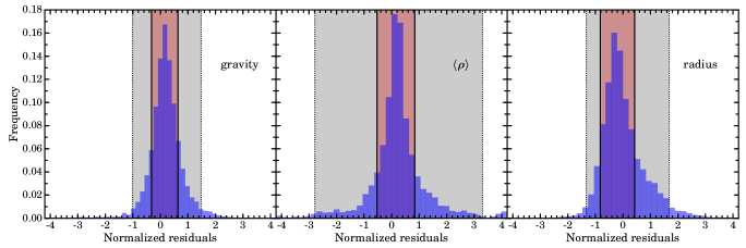
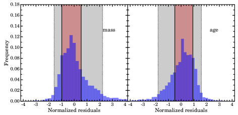
A measure of the robustness of the results returned by the GBM can be obtained by computing the difference of the central values returned by each pipeline with respect to reference values, which we take here as those returned by the combination BeSPP/GARSTEC-$\Delta\nu_{0}$, and then normalizing these differences by the median of the statistical uncertainty across all GBM pipelines. These normalized residuals give an overall picture of the scatter across different sets of GBM results. The resulting distributions for $g$, $\langle\rho\rangle$, $R$, $M$, and $\tau$ are shown in Fig. 9, including the 68.3% and 95.4% confidence levels which, in all cases except for $\langle\rho\rangle$ correspond to narrower than normal distributions of standard deviation equal to 1, i.e. when systematic and statistical uncertainties are equal.

Table 2: Uncertainties

	SDSS			ASPCAP
	Stat.	Syst.	Total	Stat.	Syst.	Total
$g$	0.025	0.009	0.028	0.025	0.016	0.030
$\langle\rho\rangle$	0.032	0.012	0.034	0.032	0.014	0.035
$R$	0.023	0.012	0.026	0.023	0.016	0.027
$M$	0.041	0.030	0.051	0.045	0.044	0.063
$\tau$	0.15	0.12	0.19	0.14	0.18	0.23

Note. — Median values of statistical, systematic and (quadratically) combined fractional uncertainties in the catalog for both $T_{\rm eff}$ scales.

The distribution of $\langle\rho\rangle$ has a slight shift introduced by the choice of reference values. The reason of the shift is related to the fact that the reference values have been computed with a grid of stellar models using $\Delta\nu_{0}$, as opposed to $\Delta\nu_{\rm scl}$ and 9 out of the 12 GBM sets of results employ $\Delta\nu_{\rm scl}$. As discussed by White et al. (2011), in the $T_{\rm eff}$ range between 5000 and 6300 K which comprises most of our sample, $(\Delta\nu_{0}/\Delta\nu_{\odot})>(\langle\rho\rangle/\langle\rho_{\odot}\rangle)^{1/2}$ whereas, by definition, $(\Delta\nu_{\rm scl}/\Delta\nu_{\odot})=(\langle\rho\rangle/\langle\rho_{\odot}\rangle)^{1/2}$. This implies that GBM relying on $\Delta\nu_{\rm scl}$ will introduce a (small) systematic shift towards higher $\langle\rho\rangle$ values than GBMs relying on the more physically correct $\Delta\nu_{0}$, as it is reflected in the distribution shown in Fig. 9. The second feature to notice is the extended tails of the distribution towards both positive and negative values that are formed by results corresponding, in all cases, to stars with very small $\Delta\nu$ uncertainties, below 0.4%. For all cases where the absolute value of the normalized residuals is larger than 2, the statistical uncertainty of $\langle\rho\rangle$ is smaller than 1.5%, a value driven by the high precision of $\Delta\nu$ for most of our sample.

The same arguments that explain the shift of peak of the $\langle\rho\rangle$ distribution are behind the shifts of the central peaks in the $R$ and $M$ distributions. The shifts here take the opposite sign with respect to the change in $\langle\rho\rangle$ because both quantities depend inversely on $\Delta\nu$ (Eqs.3-4). Finally, the age distribution simply mirrors differences in masses, as it is apparent from the lower two panels in Fig. 9. The similarity between these two distributions is, once again, reassuring in that evolutionary timescales obtained from different stellar evolution codes are in reasonably good agreement so that a given fractional difference in mass translates into a very similar fractional difference in age.

Results discussed show that differences among GBM sets of results are typically consistent with each other when measured against the statistical uncertainties, i.e. given the current limitations imposed by uncertainties in the seismic and spectroscopic data.

The systematic GBM uncertainty for each star and quantity is defined as the standard deviation $\sigma$ of the central values returned by all twelve GBM sets after applying outlier rejection. Initially, results lying beyond 3$\sigma$ of the median of the results are removed. Then, the median of the remaining sample is recalculated and the process is iterated until no values beyond the 3$\sigma$ level remain. The standard deviation of the remaining values determine the systematic GBM uncertainty.

4.3.3 ASPCAP $T_{\rm eff}$ scale

We have considered the presence of a systematic effect in the calibration of the $T_{\rm eff}$ ASPCAP scale. This is included in the present catalog as an additional systematic uncertainty in the derived stellar parameters. To obtain this uncertainty, we have performed two additional GBM runs with BeSPP/GARSTEC-$\Delta\nu_{0}$ where the ASPCAP $T_{\rm eff}$ scale has been modified by $\pm 100$ K. Then, for each stellar parameter, the systematic uncertainty has been defined as the absolute value of half the difference between those two sets of GBM results. The median fractional uncertainties for the whole sample are 1.0% ($\log{g}$), 0.3% ($\langle\rho\rangle$), 1% ($R$), 3% ($M$) and 13% ($\tau$). In the case of $M$ and $\tau$ these are smaller, but comparable, with median statistical uncertainties as discussed in Sect.4.2 whereas they are substantially smaller for the other stellar parameters.

This systematic component of the total error budget is not included in the catalog based on the SDSS griz $T_{\rm eff}$ scale. The reason, discussed in Sect. 2.1.3, is that this $T_{\rm eff}$ scale is more accurate than the ASPCAP $T_{\rm eff}$ scale.

4.4 Final uncertainties

Each quantity in the catalog includes both statistical and systematic uncertainties separately. These are assigned as follows:

• Statistical: the formal uncertainty returned by BeSPP/GARSTEC-$\Delta\nu_{0}$, the reference GBM. Positive and negative errors are quoted individually.

• Systematic: for the stellar properties based on the SDSS $T_{\rm eff}$ scale, the systematic uncertainty is equal to the GBM systematic uncertainty (Sect. 4.3.1). For stellar properties determined using the ASPCAP $T_{\rm eff}$ scale both, GBM (Sect. 4.3.1) and $T_{\rm eff}$ scale (Sect. 4.3.3) systematic uncertainties, are added in quadrature to provide the final systematic uncertainty.

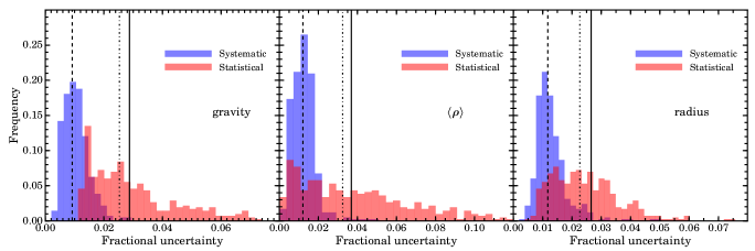
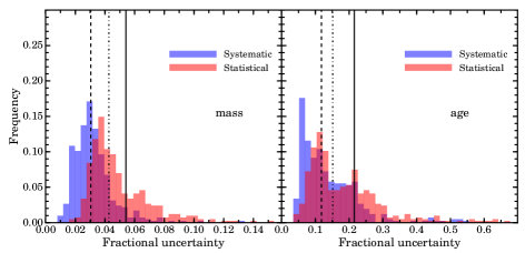
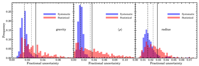
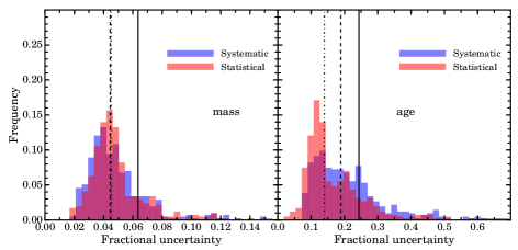
The final distributions of errors in the catalog are shown in Fig. 10 for the SDSS $T_{\rm eff}$ scale and in Fig. 11 for the ASPCAP $T_{\rm eff}$ scale. Vertical lines indicate median values for the different uncertainty components as indicated in the figure. These values are also presented in Table 2.

For the SDSS case, statistical uncertainties dominate over systematic ones for $g$, $\langle\rho\rangle$, and $R$, and $M$, whereas they are comparable for $\tau$. In the case of the ASPCAP $T_{\rm eff}$ scale, statistical uncertainties are very similar to those in the SDSS case, but systematic uncertainties are larger due to the inclusion of the $T_{\rm eff}$ systematic error (Sect. 4.3.3). This is particularly relevant for $M$ and $\tau$, for which systematic uncertainties are comparable to or dominate over the statistical uncertainties.

Figure 10: Distributions of final errors in the catalog based on the SDSS $T_{\rm eff}$ scale. Statistical (average of positive and negative) and systematic components are given separately. Median values are shown in dashed, dotted-dashed and solid lines for the systematic, statistical and quadratically combined (total) uncertainty respectively.

Figure 11: Same as Fig. 10 but for the ASPCAP $T_{\rm eff}$ scale.

5 APOKASC catalog

5.1 Presentation

The final catalog contains 415 dwarfs and subgiant stars. Their asteroseismic properties, reported in Table 3, include the global seismic quantities $\nu_{\rm max}$ and $\Delta\nu$, the length of the Kepler time series used in their determination as well as the height-to-background ratio HBR (Sect. 2.2 and Mosser et al. 2012).

Table 3: APOKASC catalog - Seismic data

KIC ID	$\nu_{\rm max}$ [$\mu$Hz]	$\Delta\nu$ [$\mu$Hz]	Length [d]	1HBR
1435467	$1382.31\pm 19.04$	$70.56\pm 0.09$	938.1	1.66
2010607	$\phantom{1}674.92\pm 146.5$	$42.48\pm 2.18$	28.9	1.55
2309595	$\phantom{1}643.21\pm 11.23$	$39.03\pm 0.72$	28.9	1.77

Note. — See text for details. The full table is available in a machine-readable form in the online journal. A portion is shown here for guidance regarding its form and content.

The seismically determined stellar quantities reported in the catalog are the radius, mass, surface gravity, mean density and age. Properties obtained using either the SDSS or the ASPCAP $T_{\rm eff}$ scales are reported separately in Tables 4 and 5 respectively. For each quantity asymmetric statistical uncertainties and a symmetric systematic uncertainty, determined as described in Sect. 4.4, are given separately.

Table 4: APOKASC dwarfs and subgiants catalog - SDSS $T_{\rm eff}$ scale

KIC ID	$T_{\rm eff}$ [K]	${\rm[M/H]}$ [dex]	Radius [${\rm R_{\odot}}$]	Mass [${\rm M_{\odot}}$]	$\log{g}$ [dex]	$\langle\rho\rangle$ [solar units]	Age [Gyr]
1435467	$6433\pm 86$	$-0.03\pm 0.10$	$1.69^{+0.01+0.01}_{-0.02-0.01}$	$1.34^{+0.04+0.02}_{-0.04-0.02}$	$4.109^{+0.006+0.002}_{-0.006-0.002}$	$0.2777^{+0.0024+0.0015}_{-0.0024-0.0015}$	$2.60^{+0.30+0.21}_{-0.29-0.21}$
2110607	$6361\pm 71$	$-0.07\pm 0.10$	$2.41^{+0.10+0.03}_{-0.09-0.03}$	$1.40^{+0.07+0.05}_{-0.05-0.05}$	$3.819^{+0.027+0.003}_{-0.027-0.003}$	$0.0997^{+0.0099+0.0014}_{-0.0094-0.0014}$	$2.75^{+0.30+0.18}_{-0.30-0.18}$
2309595	$5238\pm 65$	$-0.09\pm 0.10$	$2.42^{+0.08+0.02}_{-0.08-0.02}$	$1.17^{+0.08+0.02}_{-0.08-0.02}$	$3.736^{+0.008+0.002}_{-0.008-0.002}$	$0.0818^{+0.0025+0.0007}_{-0.0025-0.0007}$	$5.46^{+1.35+0.42}_{-1.02-0.44}$

Note. — For seismically determined stellar parameters the first error term is the statistical error (Sect. 4.2) and the second one the total systematic error (Sect. 4.3). The full table is available in a machine-readable form in the online journal. A portion is shown here for guidance regarding its form and content.

Table 5: APOKASC dwarfs and subgiants catalog - ASPCAP $T_{\rm eff}$ scale

KIC ID	$T_{\rm eff}$ [K]	${\rm[M/H]}$ [dex]	Radius [${\rm R_{\odot}}$]	Mass [${\rm M_{\odot}}$]	$\log{g}$ [dex]	$\langle\rho\rangle$ [solar units]	Age [Gyr]
1435467	$6096\pm 69$	$-0.03\pm 0.10$	$1.68^{+0.01+0.01}_{-0.01-0.01}$	$1.28^{+0.03+0.03}_{-0.03-0.03}$	$4.095^{+0.005+0.004}_{-0.005-0.004}$	$0.2711^{+0.0011+0.0015}_{-0.0010-0.0015}$	$3.75^{+0.35+0.50}_{-0.32-0.50}$
2010607	$6013\pm 69$	$-0.07\pm 0.10$	$2.39^{+0.10+0.03}_{-0.09-0.03}$	$1.33^{+0.06+0.04}_{-0.05-0.04}$	$3.802^{+0.026+0.006}_{-0.027-0.006}$	$0.0967^{+0.0097+0.0015}_{-0.0095-0.0015}$	$3.54^{+0.40+0.33}_{-0.39-0.33}$
2309595	$5000\pm 69$	$-0.09\pm 0.10$	$2.30^{+0.08+0.06}_{-0.07-0.06}$	$1.02^{+0.08+0.07}_{-0.07-0.07}$	$3.723^{+0.008+0.007}_{-0.008-0.007}$	$0.0839^{+0.0026+0.0013}_{-0.0026-0.0013}$	$9.54^{+2.67+2.52}_{-2.19-2.52}$

Note. — For seismically determined stellar parameters the first error term is the statistical error (Sect. 4.2) and the second one the total systematic error (Sect. 4.3). The full table is available in a machine-readable form in the online journal. A portion is shown here for guidance regarding its form and content.

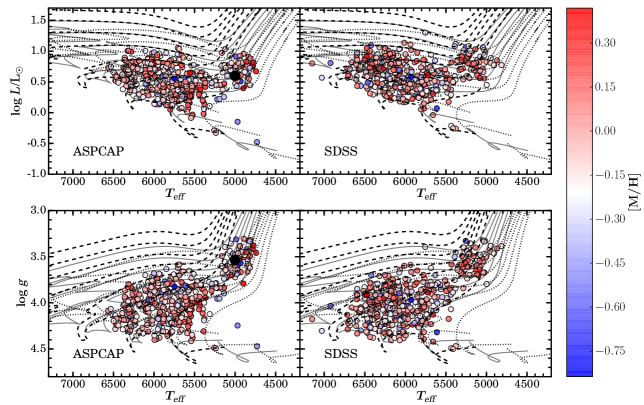
Figure 12 shows in the top panels the Hertzsprung-Russell diagrams and in the bottom panels the Kiel diagrams for the full sample and for both $T_{\rm eff}$ scales. Stars have been color coded according to their ${\rm[M/H]}$ value. GARSTEC evolutionary tracks for masses between 0.8 and 2 ${\rm M_{\odot}}$, and ${\rm[M/H]}=-0.5,0.0,0.5$ are overplotted.

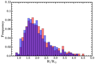
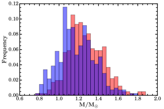
Figure 13 presents the distributions of radii and masses for the whole sample and both ASPCAP and SDSS $T_{\rm eff}$ scales. The effect of the systematic offset between the two scales is visible. This is more noticeable in the mass distribution, for which the lower ASPCAP temperatures lead to smaller stellar masses. This is discussed further in the next section.

Figure 12: Hertzsprung-Russell and Kiel diagrams of the full APOKASC sample (top and bottom panels respectively), for the spectroscopic $T_{\rm eff}$ scale (ASPCAP; left panels) and the $T_{\rm eff}$ scale based on SDSS griz photometry (right panels). The black symbol identifies a star with ${\rm[M/H]}=-1.98$ (out of the color scale for ${\rm[M/H]}$).

Figure 13: Distributions of radii and masses for the catalog for the SDSS (red) and ASPCAP (blue) $T_{\rm eff}$ scales.

5.2 Impact of the $T_{\rm eff}$ scale

The systematic differences between the ASPCAP and the SDSS $T_{\rm eff}$ scales (Sect. 2.1.3) lead to systematic variations in the seismically determined stellar parameters that we discuss here.

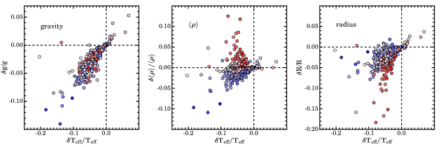
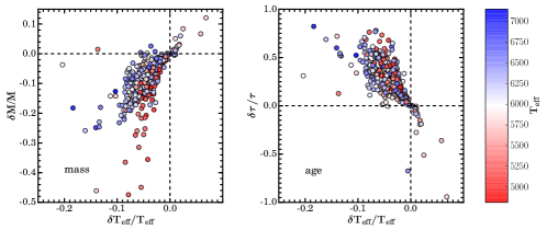
The fractional differences in the stellar parameters are shown in Fig. 14 as a function of the fractional difference $\delta T_{\rm eff}/T_{\rm eff}$. Stars are color coded according to their SDSS $T_{\rm eff}$. For $g$, the variations directly reflect the dependence of the seismic gravity on $\sqrt{T_{\rm eff}}$ (Eq. 1). Differences in $\langle\rho\rangle$ can be both positive and negative for a given $\delta T_{\rm eff}$. To first order, the scaling between $\langle\rho\rangle$ and $\Delta\nu$ does not include $T_{\rm eff}$. However, the central values in the catalog make use of $\Delta\nu_{0}$, not of $\Delta\nu_{\rm scl}$, and the difference between the two does in fact depend on $T_{\rm eff}$ as shown in Fig. 4. Due to the systematic nature of the $T_{\rm eff}$ differences between the ASPCAP and SDSS scales, the sign of $\delta\langle\rho\rangle/\langle\rho\rangle$ therefore depends, for a given star, on whether its $T_{\rm eff}$ is cooler or hotter than the $T_{\rm eff}$ value for which $\Delta\nu_{0}/\Delta\nu_{\rm scl}$ has its maximum (Fig. 4). This sets the general trend, seen in Fig. 14, that $\langle\rho\rangle_{\rm ASP}>\langle\rho\rangle_{\rm SDSS}$ for the cooler stars of the sample and the reverse effect for stars hotter than $\approx 5500$ K. For $\sim 97\%$ of the sample, changes are smaller than 5%. The median difference is $-2.3\%$ in $g$ and $-0.3\%$ in $\langle\rho\rangle$.

Changes in stellar radii have two contributions when the $T_{\rm eff}$ scale changes, one through its dependence on $\sqrt{T_{\rm eff}}$ and the other one, indirect, through the $\Delta\nu_{0}/\Delta\nu_{\rm scl}$ dependence on $T_{\rm eff}$. The two effects partially cancel each other out for stars with $T_{\rm eff}\gtrsim 5500$ K but are added in the case of the cooler stars, for which the change from the SDSS to the ASPCAP scale leads to systematically smaller $\Delta\nu_{0}/\Delta\nu_{\rm scl}$ corrections. This is reflected in Fig. 14 which shows that radii differences for cooler stars are stretched in comparison to hotter stars with similar relative $T_{\rm eff}$ variations. The median difference for stellar radii is $-1.8\%$.

Stellar masses show an analogous response to $T_{\rm eff}$ variations but the magnitude of the changes is augemented with respect to radii due to the steeper dependence of seismic mass determinations on both $\Delta\nu$ and $T_{\rm eff}$. In the case of the mass it becomes even clearer than for radius that there are two separate branches, one for hotter and one for cooler stars. Stellar ages, once again, mostly reflect the changes in the derived stellar masses. The median difference for mass is $-6.2\%$ and for age is $+35\%$.

Figure 14: Fractional variations in the seismically determined stellar parameters as a function of the relative $T_{\rm eff}$ difference between the ASPCAP and SDSS scales. Differences are in the sense ASPCAP $-$ SDSS.

5.3 Comparisons with other works

5.3.1 Chaplin et al. 2014

The vast majority of stars in the catalog presented in this work were also part of the C14 catalog. The most important difference with respect to C14 is that a single value ${\rm[Fe/H]}=-0.2\pm 0.3$, taken as representative of the solar neighborhood (Silva Aguirre et al., 2011), was adopted for the whole sample in that work. The large uncertainty effectively implied that ${\rm[Fe/H]}$ actually had a relatively minor influence on the derived stellar properties. The SDSS $T_{\rm eff}$ scale used in this work is the same used in C14.

Figure 15: Fractional variations in the seismically determined stellar parameters as a function of the ASPCAP metallicity between the SDSS-based results and those in the Chaplin et al. (2014, C14) Kepler catalog. Vertical line at ${\rm[Fe/H]}=-0.2$ denotes the fiducial value adopted for the whole sample in C14. Differences are in the sense ”this work - C14”. Linear fits are shown in blue solid lines and 1$\sigma$ variations in dashed lines. Median uncertainties of each quantity are shown on top left corners.

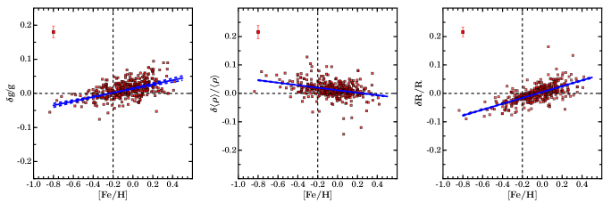
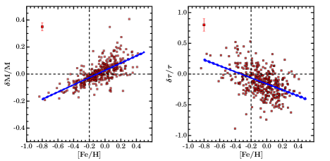
We can highlight the impact of having ${\rm[M/H]}$ measurements by directly comparing the stellar properties derived in this catalog with respect to those in C14 when the SDSS $T_{\rm eff}$ scale is used in both cases. This is shown in Fig. 15, where fractional differences are shown as a function of the ASPCAP ${\rm[M/H]}$ value. For reference, the ${\rm[Fe/H]}$ adopted in C14 is shown as a vertical dashed line. For all seismically determined stellar quantities there are clear correlations in the differences between the present and the C14 catalogs with the actual ${\rm[M/H]}$ of stars. A simple linear fit $\delta=a\cdot({\rm[M/H]}+0.2)+b$, shown in each plot together with the 1$\sigma$ variation in solid and dashed lines respectively, is indicative of the dependence of each stellar parameter on ${\rm[M/H]}$. The fits have slopes equal to $a=0.062\,(g),-0.044\,(\langle\rho\rangle),0.103\,(R),0.267\,(M),-0.493\,(\tau)$. The offsets at ${\rm[M/H]}=-0.2$ for the different quantities are $b=0.004,0.020,-0.016,-0.026,-0.062$ in the same order as above. Stellar parameters in C14 were also determined using BeSPP, models computed with GARSTEC, and $\Delta\nu_{0}$. The reason for the offset in $\langle\rho\rangle$ arises from the fact that contrary to the procedure applied in the present work, in C14 $\Delta\nu_{0}$ in the stellar models were not rescaled according to the factor $f_{\Delta\nu}$ described in Sect. 4.1. This leads to a 1% offset in $\Delta\nu_{0}$ between the two stellar models grid that propagates as about twice that value to the $\langle\rho\rangle$ determination, as expected, with a comparable offset for $R$ and a slightly larger one for $M$ which, in turn, propagates into a $\tau$ offset. The scatter seen in the relations can have at least three sources: the asteroseismic data used here is determined in many cases from longer time series and improved seismic analysis, and the grids of models have not been computed with the exact same assumptions, the current version of BeSPP is an evolution of that used in C14, when it was still based on a frequentist approach akin to that used by the YB pipeline.

As a whole, results in this catalog are consistent with those previously published by C14, but represent a qualitative and quantitative step forward because metallicity information is now included individually for all stars. The C14 catalog, however, includes about 100 more stars that were not observed with APOGEE (see Sect. 2).

5.3.2 The LEGACY Sample

The LEGACY Sample is formed by 66 main sequence stars of highest quality of asteroseismic data from the Kepler mission (Lund et al., 2017). Asteroseismic analysis of these stars is based on stellar model fitting that relies on using specific combinations of individual frequencies that allow a more precise determination of stellar parameters. Detailed results have been presented in Silva Aguirre et al. (2017).

From the total common sample between APOKASC and LEGACY, we have removed two stars because in one case the ASPCAP $T_{\rm eff}$ and in the other the SDSS $T_{\rm eff}$ values differ from the LEGACY $T_{\rm eff}$ value (based on SPC spectroscopic analysis by Buchhave & Latham 2015) by more than 600 K. In total, we are left with a common sample of 45 stars that can be used as a benchmark. Our comparison of stellar parameters makes use of LEGACY results computed with the BASTA pipeline, which are based on GARSTEC. By using LEGACY results based on the same evolutionary code used to determine the central values in the APOKASC catalogs, we minimize the systematic differences arising from stellar models.

Note that, in addition to the different type of input seismic data used in this catalog ($\Delta\nu$ and $\nu_{\rm max}$) and in the LEGACY work (individual frequencies or frequency separation ratios), another source of deviation between the two sets of results is likely due to the fact that all GBM presented in this work are based on libraries of stellar models where the mixing length parameter is fixed, whereas in the LEGACY work this is an additional free parameter in the stellar models. This precludes a detailed discussion of star-by-star comparions. Instead, we focus on a global comparison of mean differences and dispersions.

Figure 16: Comparison of the APOKASC results against the LEGACY sample for all stars common to both samples. Red squares (blue circles) refer to results obtained with the SDSS (ASPCAP) $T_{\rm eff}$ scale. Red and blue horizontal lines show the weighted mean differences (solid) and rms (dashed) with respect to the LEGACY sample for each $T_{\rm eff}$ scale (see Table 6).

Table 6: APOKASC$-$LEGACY

	ASPCAP				SDSS
	Weig. Mean	Weig. rms	Unw. Mean		Weig. Mean	Weig. rms	Unw. Mean
$\delta g/g$	$-0.007$	0.028	$-0.002$		$-$0.014	0.021	$-$0.016
$\delta\langle\rho\rangle/\langle\rho\rangle$	$-0.004$	0.013	$-5\times 10^{-4}$		$-$0.001	0.014	$-$0.007
$\delta R/R$	$-0.004$	0.018	$-0.001$		$-$0.007	0.016	$-$0.009
$\delta M/M$	$-0.015$	0.061	$-$0.003		$-$0.027	0.047	$-$0.036
$\delta\tau/\tau$	$-$0.078	0.300	$-$0.213		$-0.167$	0.183	$-0.116$

Note. — Comparison of APOKASC and LEGACY results shown as APOKASC–LEGACY. Weighted mean and rms fractional differences are shown for both $T_{\rm eff}$ scales used in this work. Additionally, the unweighted fractional mean differences are also given.

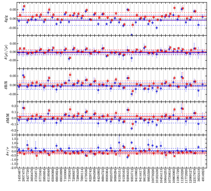
Figure 16 shows the comparison for all stars and both $T_{\rm eff}$ scales, identifying in blue (circles) results for the SDSS $T_{\rm eff}$ scale and in red (squares) those for the ASPCAP $T_{\rm eff}$ scale. Horizontal lines indicate the weighted mean difference with respect to the LEGACY results. For three stars only ASPCAP $T_{\rm eff}$ values are available.

The weighed mean and the dispersion (rms) of the fractional differences of the two APOKASC sets of results with respect to the LEGACY results are summarized in Table 6. For all stellar parameters, ASPCAP results show a smaller mean difference than SDSS. Overall, it is reassuring that the systematic offsets between APOKASC and LEGACY results are in all cases substantially smaller than the median error of each quantity in the APOKASC catalog (Figs. 10 and 11).

In the following we discuss the comparison in more detail, in particular for stellar mass. The mean fractional difference $\delta M/M$ between APOKASC/ASPCAP and LEGACY is $-1.5\%$ and between APOKASC/SDSS and LEGACY is 2.7%. The mean $T_{\rm eff}$ in ASPCAP is 1.4% cooler than in the LEGACY sample, and the SDSS $T_{\rm eff}$ scale is 1.3% hotter. By propagating these differences through the scaling relation Eq. 3, we infer that asteroseismic masses from global seismology show a systematic mean deviation of about 2% with respect to the LEGACY sample. We have confirmed this by performing an additional GBM run with BeS/G-$\Delta\nu_{0}$ using as inputs the combination of our global seismic parameters and the $T_{\rm eff}$ and ${\rm[Fe/H]}$ values used from LEGACY sample (Silva Aguirre et al., 2017). In this case, we find that the mean $\delta M/M=0.6\%$, in agreement with the above estimate, and an rms $\delta M/M=6\%$. In this case, the mean and rms values for $\delta\tau/\tau$ are -4% and 26%, respectively. These numbers can be taken as a first order estimation of the systematic differences in mass and age results between global seismology and more detailed analysis based on modeling many individual mode frequencies. However, a more careful analysis required to be more conclusive is beyond the scope of this paper. For example, global seismic parameters reported for the LEGACY sample (Lund et al., 2017), are not the same as the ones in our work ($\nu_{\rm max}$ in particular is different by up to a few percent for some stars) and we have not tested if this introduces systematic effects. Also, despite that stellar models are computed with GARSTEC in both cases, they are not exactly the same.

From Table 6 we also see that the mass and age rms are larger for the ASPCAP results than for SDSS. For the ASPCAP results, the larger rms is driven by three stars with $T_{\rm eff}$ values different from the LEGACY values by more than 300 K. By removing these stars the rms decreases to 6.3%, around the 6% found between global and detailed seismic analysis. Mass differences (global$-$detailed seismology) do not show clear correlation with the $T_{\rm eff}$ differences in the analysis. However, age differences do correlate with the $T_{\rm eff}$ scale. This explains in part the variation in $\delta\tau/\tau$ from almost 8% (ASPCAP) down to -17% (SDSS), which is larger than expected from the differences found for $\delta M/M$. A detailed comparison between global and detailed seismic analysis is worth further investigation.

Figure 17: Left panel: comparison between seismic and flickering gravities from Bastien et al. (2016). A typical error bar is shown for orientation. The black square is KIC 7341231, with ${\rm[M/H]}=-1.97$. Right panel: residuals as a function of [M/H]  and a linear fit signaling a possible, albeit mild, trend in flickering gravities with [M/H]. Squares indicate stars for which residuals are larger than 0.2 dex and are excluded from the fit.

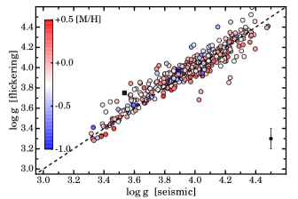
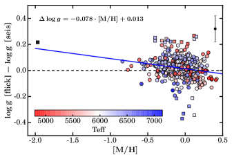
A final and useful comparison between the APOKASC catalog and the LEGACY results is that of the typical errors with which the different stellar quantities can be determined based on global seismic parameters (APOKASC) or on using individual frequencies. The error distributions presented in Silva Aguirre et al. (2017) (see their Figure 2) are the equivalent of the statistical errors in the APOKASC catalog. Following the publication of the original LEGACY work (Lund et al., 2017), an error was identified in the preparation of the frequency ratios (Roxburgh, 2017; Lund et al., submitted), which caused an overestimation of uncertainties in the LEGACY results determined with some of the pipelines used in Silva Aguirre et al. (2017). Taking this factor into account (Silva Aguirre private comm.), typical errors embracing LEGACY results obtained with all pipelines range between 0.5-1% for $\langle\rho\rangle$, 0.8-1.8% for $R$, 2-4% for $M$, and 5-10% for $\tau$. The statistical errors in the catalog presented in this paper (see Tab. 2 and Fig. 6) are about 3% ($\langle\rho\rangle$), 2.3% ($R$), 4% ($M$), and 15% ($\tau$). The better precision of the detailed seismic analysis is most evident for $\langle\rho\rangle$, while for $R$ and $M$ results are closer. For $\tau$, the precision of global seismology is on average a factor of two larger than detailed seismic analysis. We note that the final errors in the present catalog include the systematic component to the total uncertainty, whereas in Silva Aguirre et al. (2017) this has not been included in the error estimate because results for all seismic pipelines were reported.

According to our results, the precision of global seismology is typically larger than that of detailed seismology by factors from about 1.5 to 3, depending on the stellar property considered. Note that in this discussion, the APOKASC results include stars with timeseries of all available lengths. On the other hand, the LEGACY sample is formed by the best available Kepler data.

The overall comparison of the APOKASC catalog, with both $T_{\rm eff}$ scales, against the LEGACY sample shows there are no strong systematic differences present at levels larger than the mean uncertainties in the catalog. Moreover, the typical precision with which GBM pipelines estimate stellar parameters using only $\Delta\nu$ and $\nu_{\rm max}$ is comparable to those obtained using individual oscillation frequencies, at least when stars without mixed-modes are considered. More detailed work is however desirable to understand in full the limitations of global seismology of dwarf and subgiant stars.

5.3.3 Gravities from flickering

Timescales and amplitudes of granulation are tightly related to surface gravities (Kjeldsen & Bedding, 2011), which was first observed for red giants (Mathur et al., 2012) and later applied to measure surface gravities of dwarfs and giants from long-cadence data. The so-called flicker method (Bastien et al., 2013) is based on a correlation between the rms variations of the stellar brightness on timescales shorter than 8 hours, the so-called 8-hr flicker $F_{8}$, and the surface gravitity of stars. The relation between $F_{8}$ and $\log{g}$ was further calibrated and analyzed in Bastien et al. (2016), using in part seismic $\log{g}$ from C14.

As discussed in Sect. 5.3.1, the availability of [M/H] from APOGEE leads to changes in the determined seismic $\log{g}$ values with respect to C14, although these corrections are small in comparison with the typical $0.10$ dex uncertainties in $\log{g}$ obtained from $F_{8}$. Left panel in Figure 17 compares the newly determined seismic $\log{g}$ with the $F_{8}$ $\log{g}$ from Bastien et al. (2016) with symbols coded according to stellar metallicity. The agreement of the flickering gravities with the newly determined seismic gravity is excellent overall, with a mean difference of 0.017 dex (flickering$-$seismic) and a dispersion of 0.068 dex for the whole APOKASC sample. If the C14 $\log{g}$ values are used instead for the same sample, the mean and dispersion of the difference are 0.023 dex and 0.071 dex respectively. Including the [M/H]  information brings both $\log{g}$ scales (slightly) closer.

Figure 18: The left panel shows fractional differences of the catalog radii with respect to TGAS radii (Huber et al., 2017) for ASPCAP (blue) and SDSS (red) $T_{\rm eff}$ scales (in the sense APOKASC$-$TGAS). The right panel shows differences normalized to the combined uncertainties, $\sigma_{\rm tot}=\sqrt{\sigma^{2}_{cat}+\sigma^{2}_{TGAS}}$. Vertical lines show median values for ASPCAP (dashed) and SDSS (solid) samples.

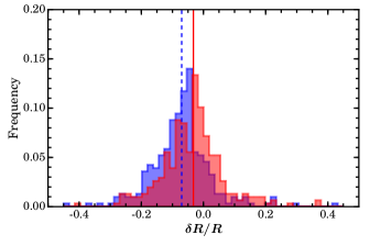
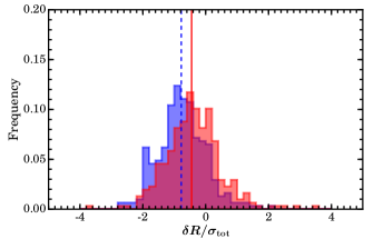
More interesting is perhaps the difference between the flicker and the seismic gravities ($\Delta\log{g}$) as a function of [M/H] that is shown in the right panel in Fig. 17, where colors are the same as in the left panel. Here, stars showing $|\Delta\log{g}|>0.2$ dex ($\sim 2\sigma_{\rm F_{8}}$) are plotted with squares. The larger negative differences are related to some of the hotter stars in the sample, above $\approx 6500$ K; as pointed out in Bastien et al. (2016), the tight relation between $F_{8}$ and $\log{g}$ seems to break down around this or slightly higher $T_{\rm eff}$. We have performed a linear fit to $\Delta\log{g}$ as a function of [M/H], excluding from the fit all cases where $|\Delta\log{g}|>0.2$ dex. The metal-poor star KIC 7341231, shown with a black square, is also excluded from the fit. The result is plotted as a blue solid line. We have also carried out linear fits to binned data. This was done by sorting stars by increasing [M/H]  computing the mean [M/H] and $\Delta\log{g}$ in batches of 10 stars and then performing the linear fit. The result is virtually unchanged compared to the one reported in Fig. 17. We have checked that results are not significantly affected by the bin size. Interestingly, the linear fit reproduces well the result for KIC 7341231, although the typical scatter in flicker gravities prevents us from drawing firm conclusions.

The significance of the correlation between $\Delta\log{g}$ and ${\rm[M/H]}$ has been tested by computing the Kendall’s $\tau_{K}$ non-parametric correlation test. Applying the cut $|\Delta\log{g}|>0.2$ dex we obtain for 381 stars $\tau_{K}=0.177$, leading to $z_{K}=5.16$ and a p-value= $1.2\times 10^{-7}$. If stars are grouped in 12 bins of 30 stars each, then $\tau_{K}=0.522$, i.e. $z_{K}=2.47$ or a p-value= $6.7\times 10^{-3}$). A highly significant correlation between $\Delta\log{g}$ and ${\rm[M/H]}$ exists in both cases.

The result above seems to suggest there is some degree of correlation between the level of flickering activity $F_{8}$ and the metallicity of the star for dwarfs and subgiants. As [M/H] decreases, the tendency is for $F_{8}$ to lead to larger estimates of $\log{g}$ than the seismic values. Based on the $F_{8}-\log{g}$ relation in Bastien et al. (2016), this impies lower levels of activity associated with lower [M/H]. This is in qualitative agreement with theoretical models (Samadi, 2011) linking F8 and mode amplitudeswith ${\rm[M/H]}$ and recent detailed analysis of red giant stars carried out by Corsaro et al. (2017) based on open star clusters. The relation between stellar activity, in particular as measured by $F_{8}$, metallicity, and $\log{g}$ deserves further and detailed study.

5.3.4 Comparison with TGAS radii

Recently, Huber et al. (2017) have used the Gaia DR1 (TGAS) parallaxes in combination with the 2MASS-K band and $T_{\rm eff}$ from Buchhave & Latham (2015) to determine stellar radii. Almost all stars in the catalog in this paper have been analyzed in Huber et al. (2017) and form their dwarf and subgiant sample. Figure 18 shows histograms comparing stellar radii for our two $T_{\rm eff}$ scales with radii determined from TGAS by Huber et al. (2017) using the same $T_{\rm eff}$ scales. The median differences, indicated by vertical lines, are 3.3% and 7.0% for the SDSS and the ASPCAP $T_{\rm eff}$ based results respectively, with a dispersion in both cases of 10%. This offset was already highlighted by Huber et al. (2017), who concluded that TGAS results favor a hotter $T_{\rm eff}$ scale such as the SDSS scale rather than the cooler one provided by ASPCAP. The right panel shows differences normalized with respect to the combined APOKASC + TGAS uncertainty, where the offsets are also visible. The dispersion of uncertainties is 0.9$\sigma$ and 1$\sigma$ for the ASPCAP and SDSS scales respectively, and it is dominated by errors in the TGAS results.

Our results confirm those in Huber et al. (2017), that asteroseismic radii agree with those determined from Gaia parallaxes. However, there is a systematic offset present, and its nature is not fully understood. It might be tempting to present this as a limitation of global seismology (i.e. based on $\Delta\nu$ and $\nu_{\rm max}$), stellar models (i.e. shortcomings in determination of $\Delta\nu_{0}$), or on the scaling relation of $\nu_{\rm max}$. But, our radii compare very well with those from the LEGACY sample (Sect. 5.3.2), determined from a seismic analysis based on oscillation frequencies. In fact, seismic parallaxes of the LEGACY sample computed by Silva Aguirre et al. (2017, see their Figure 13) show a systematic offset of $\sim 0.25$ mas towards larger values than those from TGAS. Analogous results were also found by Davies et al. (2017) using asteroseismic parallaxes of red clump stars and by Stassun & Torres (2016) using binaries. Because seismic parallaxes are based on computing the total stellar flux, results in Silva Aguirre et al. (2017) are equivalent to having seismic radii smaller than TGAS radii, consistent with our findings. About 2% of the offset in radius can be accounted for by a systematic offset in TGAS parallaxes. Still, further study is required to have a better understanding of whether the reasons for the offset lies with asteroseismic analysis, $T_{\rm eff}$ scale, or a systematic underestimation of TGAS parallaxes. Gaia DR2 will certainly help shed light on this.

Figure 19: Left panel: ASPCAP vs Bruntt et al. (2012) $v\sin{i}$. Right panel: $v\sin{i}$ vs $T_{\rm eff}$ for the whole APOKASC sample, M67 stars, and Hyades and Praesepe stars from van Saders & Pinsonneault (2013). Main sequence APOKASC stars are color coded according to their mass.

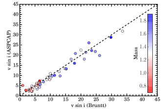
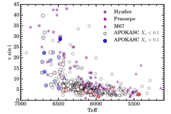
5.3.5 Projected rotational velocities

The synthetic grid of spectra in ASPCAP incorporates rotational broadening as an additional dimension in the analysis since DR13. The possibility of having a large sample of stars with $v\sin{i}$ determinations and seismic parameters, even if the inclination $i$ remains unknown, opens up interesting possibilities for studies of gyrochronology, at least in a statistical sense. In order to assess the quality of ASPCAP $v\sin{i}$ determinations, we use stars in common with Bruntt et al. (2012) for which $v\sin{i}$ has been determined from optical spectroscopy taken at resolution R$\sim 80000$ and S/N $>200$. Results are shown in the left panel of Figure 19, where stars are color coded according to their mass. There is a very good agreement between both datasets, with a dispersion of $1.8\ \hbox{km/s}$ between the two datasets and a mean offset of $-0.5\ \hbox{km/s}$ (in the sense ASPCAP$-$Bruntt).

The comparison above lends strong support to $v\sin{i}$ determinations with ASPCAP. There are 331 stars in the catalog with ASPCAP $v\sin{i}$ determinations and they are shown in the right panel of Figure 19 where $v\sin{i}$ is shown as a function of $T_{\rm eff}$ (SDSS). We have excluded from the plot stars that have been flagged by ASPCAP with problematic $v\sin{i}$. These are mostly stars with low ($\sim 2~{}\hbox{km/s}$) $v\sin{i}$. Main sequence stars are shown as large filled circles, color coded as in the left panel of the figure. Stars that are close to the end of the main sequence or have already evolved off it are shown as small open circles. This is an approximate classification based on whether the central hydrogen mass fraction $X_{c}$, estimated from the BeS/G-$\Delta\nu_{\rm scl}$ GBM results, is larger or smaller than 0.1. The plot includes ASPCAP values of $v\sin{i}$ for M67 stars. Hyades and Praesepe stars from van Saders & Pinsonneault (2013) are also included. For all three clusters, $T_{\rm eff}$ have been determined using $(B-V)$ colors and the Casagrande et al. (2010) transformation. The general trend in the APOKASC sample is similar to that seen in cluster stars. Cool stars ($T_{\rm eff}<6200$ K) show slow rotation in all but a few cases. Above this temperature, as surface convective envelopes thin, magnetic braking becomes less effective and higher rotation rates are present, as in cluster stars (van Saders & Pinsonneault, 2013). At $T_{\rm eff}>6200$ K there seems to be an excess of low $v\sin{i}$ in comparison to cluster stars. This may be indicative that there is a relative lack of fast rotators in seismic samples (Tayar et al., 2015) and the particular exclusion of close binary stars, which, at least for red giant stars, tend to have rapid rotation but suppressed oscillations (Gaulme et al., 2014). Ongoing work includes the comparison of estimated $v\sin{i}$ distributions obtained for stars with known rotational periods to further confirm the reliability of $v\sin{i}$ determinations by ASPCAP (Simonian et al. in prep.).

6 Summary

This work extends the first APOKASC red giants catalog presented in Pinsonneault et al. (2014) to include 415 dwarf and subgiant stars. It is based on global seismic parameters $\Delta\nu$ and $\nu_{\rm max}$ obtained from Kepler short cadence asteroseismic data with length of lightcurves spanning from 30 up to 1055 days. Adopted seismic values are from the SYD pipeline (Huber et al., 2009), and four other pipelines have been used to estimate systematic uncertainties in $\Delta\nu$ and $\nu_{\rm max}$. Two $T_{\rm eff}$ scales have been used throughout this work, a spectroscopic scale based on the $H$-band spectra taken by APOGEE (Majewski et al., 2015) and the other one based on SDSS griz photometry (Pinsonneault et al., 2012). APOGEE data have been reduced using ASPCAP, in the version corresponding to the SDSS-IV DR13 (Albareti et al., 2016), from which we have also taken the metallicity [M/H] used in combination with both $T_{\rm eff}$ scales. Typical $T_{\rm eff}$ uncertainties are about 70 K both for ASPCAP and SDSS scales. The formal [M/H]  uncertainty in ASPCAP is 0.03 dex, but we have expanded it to 0.1 dex to account for possible systematic errors.

The catalog includes the stellar quantities, $g$, $\langle\rho\rangle$, $R$, $M$, and $\tau$ determined with GBM techniques. In total, twelve different combinations of GBM pipelines and sets of stellar evolution tracks have been used. Central values in the catalog are from BeS/G-$\Delta\nu_{0}$ (Table 1). Each quantity is accompanied by assymetric statistical errors (those coming from uncertainties in the input data) and a symmetric systematic uncertainty that captures the dispersion of results across GBM pipelines. In the case of ASPCAP results an additional systematic component, computed by redetermining all stellar quantities using as input $T_{\rm eff}$ the ASPCAP values $\pm 100$ K, has been added in quadrature to the systematic component from the GBM pipelines. The median total uncertainties in the catalog are (SDSS/ASPCAP): 2.3/2.3% ($g$), 2.8/2.7% ($\langle\rho\rangle$), 2.1/2.4% ($R$), 4.4/5.5% ($M$), and 17/21% ($\tau$).

Stellar properties in the catalog compare well with other published data, most notably with the asteroseismic results of the LEGACY sample (Silva Aguirre et al., 2017), that are based on a more detailed asteroseismic analysis which employs individual frequencies rather than just two global quantities. Our results show small systematic offsets for all stellar quantities and the ASPCAP $T_{\rm eff}$ scale and, for the SDSS scale, a 3.6% mean offset for $M$ and a $-15.6$% offset for $\tau$, still smaller than the typical uncertainties in the catalogs. We have checked that about half these offsets are due to the SDSS $T_{\rm eff}$ scale being 1.4% hotter than the LEGACY $T_{\rm eff}$ scale. The overall agreement between our global seismic results and the more detailed LEGACY work is remarkable considering how much less information is contained in global seismology than in individual frequencies. Prospects for accurate determination of stellar properties of dwarfs and subgiants with the TESS mission, that will observe most stars for 27 days and in many cases will allow measuring only $\Delta\nu$ and $\nu_{\rm max}$, are excellent.

We have also compared the statistical uncertainties of our derived stellar parameters with those in the LEGACY sample and find them comparable. In fact, our statistical uncertainties are comparable to the most pesimistic uncertainties in Lund et al. (2017); Silva Aguirre et al. (2017) for $R$ and $M$, and larger by factors between 1.5 and 3 for $\langle\rho\rangle$ and $\tau$. The good performance of global seismology is due to the rather small fractional uncertainties in $\Delta\nu$ and $\nu_{\rm max}$ in comparison to those of the frequency separation ratios used by several pipelines in LEGACY. Error propagation from individual frequencies, even they are measured to levels of 0.1% or better, lead to uncertainties in frequency ratios that range typically between a few up to 20%. It is then apparent that a better understanding of the surface correction term continues to be searched for, because only by being able to perform seismic modeling based on individual frequencies will unleash the full power of detailed seismology.

The importance of ${\rm[M/H]}$ for determination of stellar properties from global seismic measurements is made explicit in the comparison of our results with those in C14. We have derived approximate linear relations between ${\rm[M/H]}$ and fractional variations in stellar properties such that $\delta\log{g}=0.062\,\delta{\rm[M/H]}$, $\delta\langle\rho\rangle/\langle\rho\rangle=-0.044\,\delta{\rm[M/H]}$, $\delta R/R=0.103\,\delta{\rm[M/H]}$, $\delta M/M=0.267\,\delta{\rm[M/H]}$, and $\delta\tau/\tau=-0.493\,\delta{\rm[M/H]}$.

Finally, our stellar radii have been compared with those inferred from the TGAS parallaxes (Huber et al., 2017). We confirm previous results and find an overall good agreement between asteroseismic and TGAS radii but with a systematic shift of TGAS radii being $\sim 3\%$ larger than seismic radii for the SDSS $T_{\rm eff}$ scale. This is in agreement with the analysis by Silva Aguirre et al. (2017) using different seismic information. Assuming no systematic errors in asteroseismic radii and $T_{\rm eff}$ scales, this would indicate that TGAS parallaxes are systematically underestimated by $\sim 3\%$.

We have presented the first large-scale catalog of dwarf and subgiants with seismically inferred stellar parameters and individual metallicity measurements. The detailed information on the composition of these stars obtained and released as part of DR13 makes this APOKASC catalog a unique data source for stellar studies.

Appendix A Description of stellar models

This appendix gives details of the physical inputs in the grids of stellar models that have been used in the GBM pipelines used in this work. Overall, 7 different grids of models have been used based on 6 stellar evolution codes. Two grids have been computed with GARSTEC but with different physical inputs and assumptions regarding chemical composition of the grid. The implementation of a grid of stellar models might be different for each GBM pipeline, e.g. some pipelines interpolate the original grid to have a denser coverage of the parameter space; these details have been discussed in the main body of the paper (Sect. 3). The basic references for each stellar code are: GARSTEC - Weiss & Schlattl (2008), CESTAM2k - Morel & Lebreton (2008), MESA - Paxton et al. (2013), BASTI - Pietrinferni et al. (2004), ASTEC - Christensen-Dalsgaard (2008), YREC2 - Demarque et al. (2008).

The most important information has been summarized in Tables 7 and 8. The first table lists quantities related to calibrations. All grids use variants of the Mixing Length Theory (MLT; Böhm-Vitense, 1958; Kippenhahn & Weigert, 1990) except CESTAM2k that employs the Full Spectrum Theory (FST; Canuto et al., 1996). In both cases there is a free parameter that relates the mixing length to the pressure scale height, $\Lambda=\alpha_{c}H_{P}$, with $c$ denoting either MLT or FST. This parameter is determined in all grids from a solar calibration. The MLT is not a uniquely defined theory because, in addition to the mixing length parameter ($\alpha_{\rm MLT}$) other free parameters are present (see e.g. Salaris & Cassisi 2008). Moreover, a solar calibration of $\alpha_{\rm MLT}$ depends on other physical inputs of the models such as the inclusion and efficiency of microscopic diffusion, low-temperature opacities, model atmosphere and the reference solar composition. Therefore, the $\alpha_{c}$ values are given mostly for reference but not for direct comparison among each other.

Each set of models also use a different relation to determine the initial composition of models, although they all assume a linear relation between the initial metal and helium mass fractions, i.e. $Y_{\rm ini}=(\Delta Y/\Delta Z)\cdot Z_{\rm ini}+Y_{\rm R}$. For each grid, $Y_{\rm R}$ and $\Delta Y/\Delta Z$ are included in the table. With the exception of ASTEC, these choices lead to a small range of $Y_{\rm ini}$ values for any given $Z_{\rm ini}$. The distribution of metals is determined by the adopted solar mixture, and all grids are based either on GN93 or GS98, two solar mixtures with more similarities than differences. Finally, the definition of [Fe/H]=0 associated with each grid is also listed. This is necessary because stellar models depend on the absolute $Z$ and a zero point relating $Z$ (or $Z/X$) with ${\rm[Fe/H]}$ is needed to place stellar models onto the observational plane.

Table 7: Reference quantities

Grid	Reference values
	Conv. Theory	$\alpha_{c}$	YR	$\Delta Y/\Delta Z$	Mixture	[Fe/H]=0
GARSTEC/BASTA	MLT	1.791	0.248	1.4	GS98	$Z/X=0.0230$
GARSTEC/BeSPP	MLT	1.798	0.2485	1.17	GN93	$Z/X=0.02439$
CESTAM2k	FST	0.707	0.245	1.45	GS98	$Z/X=0.02293$
MESA	MLT	1.908	0.245	1.45	GS98	$Z/X=0.02293$
BASTI	MLT	1.913	0.245	1.4	GN93	$Z/X=0.0245$
ASTEC	MLT	1.800	0.300	$-$1	GN93	$Z=0.0188$
YREC2	MLT	1.826	0.245	1.54	GS98	$Z/X=0.0230$

Note. — See text for detailed meaning of each column.

Table 8 lists inputs to stellar models describing physical inputs. Microscopic diffusion is included only in the GARSTEC models used in combination with BeSPP. The basic prescription is that from Thoul et al. (1994), but these models also include extra mixing (generically linked to turbulent mixing) below the convective envelope that moderate the efficiency of gravitational settling of helium and metals as suggested by solar models (Delahaye & Pinsonneault, 2006; Villante et al., 2014) and required for low metallicty stars (Richard et al., 2002). This is modeled according to the parametrization of VandenBerg et al. (2012), that links the macroscopic diffusion coefficient to the density at the base of the convective envelope and the mass thickness of the convective envelope.

Table 8: Physical inputs

Grid	Diffusion	Core OV	Nucl. rates	High/low-$T$ opac.	EoS
GARSTEC/BASTA	No	$f=0.016$+geom.cut	NACRE+LUNA	OPAL/F05	OPAL05
GARSTEC/BeSPP	Yes+extra mixing	$f=0.016$+geom.cut	A11	OPAL/F05	FreeEOS
CESTAM2k	No	No	NACRE	OPAL/F05	OPAL05
MESA	No	No	NACRE	OPAL/F05	OPAL05
BASTI	No	No	NACRE	OPAL/AF94	FreeEOS
ASTEC	No	No	BP95	OPAL/K91	E73
YREC2	No	0.2 $H_{P}$	A98+LUNA	OPAL/F05	OPAL05

.

Note. — See text for detailed meaning of each column. NACRE: Angulo et al. (1999), LUNA: Formicola et al. (2004); Marta et al. (2008), A11: Adelberger et al. (2011), BP95: Bahcall et al. (1995), A98: Adelberger et al. (1998), OPAL: Iglesias & Rogers (1996), F05: Ferguson et al. (2005), AF94: Alexander & Ferguson (1994), K91: Kurucz (1991), OPAL05: Rogers & Nayfonov (2002), FreeEOS: Cassisi et al. (2003), E73: Eggleton et al. (1973). Note that A11 recommended value for ${\rm{}^{14}N(p,\gamma)^{15}O}$ is that from LUNA Marta et al.,2008

Convective core overshooting (core OV) is included in some sets of models. In YREC2 models, this is done as an extension of the convective core by a fixed fraction of the pressure scale height. In GARSTEC, chemical mixing is treated as a diffusive process and overshooting at all boundaries of convective regions is applied by means of an exponentially decaying diffusive coefficient (Freytag et al., 1996). The free parameter $f$ is adjusted such that it is roughly equivalent to 0.2-0.25 $H_{\rm P}$ for convective cores of main sequence stars. Note that $H_{\rm P}$ tends to infinity for convective cores approaching zero extension. In order to avoid such unphysical situation, i.e. a tiny small convective core with an infinite overshooting region, a geometric suppression is added in the calculation of the diffusion coefficient (see Magic et al. 2010 for details).

Nuclear reaction rates come from a variety of sources. But, in this work we are only concerned about hydrogen burning processes and among all rates involved in the pp-chains and CNO-bicycle the only relevant difference between the stellar codes is the adoption, or not, of the LUNA results (Formicola et al., 2004; Marta et al., 2008) for the ${\rm{}^{14}N(p,\gamma)^{15}O}$ rate. This is done in both sets of models computed with GARSTEC (Adelberger et al. 2011 rate for this reaction is taken from the LUNA value available at that time, Marta et al. 2008) and also with YREC2. The LUNA rate for this reaction is roughly a factor of a half compared to the NACRE (Angulo et al., 1999) or the BP95 (Bahcall et al., 1995) values and the most relevant impact on stellar models used in this work is that the transition from pp-chain dominated evolution to CNO-bicycle dominated evolution is shifted towards slightly larger masses. As a result, the stellar mass at which convective cores start to develope is also slightly larger, by 0.07 ${\rm M_{\odot}}$ approximately (e.g. Magic et al., 2010).

Radiative opacities in stellar interiors are from OPAL (Iglesias & Rogers, 1996) in all cases. Low-temperature opacities are in most cases from Ferguson et al. (2005), but those from Alexander & Ferguson (1994) and Kurucz (1991) are also used. It must be noted, however, that most of the differences that might arise from using different low-temperature opacities are absorbed by using an $\alpha_{c}$ value that is solar calibrated. This is true because we are concerned with the modeling of main sequence and subgiant stars, i.e. with stars that are not very cool and far from solar conditions such that different combinations of low-temperature opacities and calibration of convection start to produce strongly deviant stellar models.

Finally, the equation of state (EoS) is also different. Some codes use the OPAL EoS (Rogers & Nayfonov, 2002) in its 2005 release, some an updated version of the FreeEOS (Cassisi et al., 2003) and ASTEC employs the simpler EoS developed by Eggleton et al. (1973).

It is not our goal here to delve into the detailed changes in the estimated stellar properties that occur due to variations in the physical inputs of models. Instead, we just present the results obtained for all stellar quantities from all GBM pipelines and assume the scatter as a measure of systematic uncertainties associated, at least partially, to uncertainties in the physical inputs of stellar models as it is discussed in Sect. 4.3.1.

Appendix B GBM Comparisons

This appendix shows detailed comparisons of results for different pairs of GBM calculations for the five stellar quantities seismically determined: $g$, $\langle\rho\rangle$, $R$, $M$, and $\tau$. There are twelve different sets of GBM results that, as described in Sect. 4.3, are used to derive systematics uncertainties. Results shown here are based on the SDSS $T_{\rm eff}$ scale but those based on the ASPCAP $T_{\rm eff}$ scale portrait the same picture.

Figures 20-24 compare one-to-one GBM results where fractional differences (in dex for $\log{g}$) are plotted as a function of $T_{\rm eff}$. In each subplot, differences are computed in the sense $(q_{r}-q_{c})/q_{c}$, where $q$ is any seismic quantity (except $\log{g}$, for which the denominator is obviously omitted) and the subindices $r$ and $c$ represent the GBM identifying the row or column respectively, e.g. the top leftmost panel shows differences in the sense YB/B$-$SPB/B. The list of all sets of GBM results is given in Table 1 in the main body of the article.

Figure 20: One-to-one comparisons of different GBM sets of results. Differences are computed in the sense ($\delta\log{g}=\log{g}_{r}-\log{g}_{c}$), where $c$ and $r$ denote, respectively, the GBM identifying the column and the row of each subplot. Red lines show the median formal error of the pipeline $r$ in 60 K $T_{\rm eff}$ bins. Results shown here are based on the SDSS $T_{\rm eff}$ scale. GBM labels are given in Table 1.

GBM comparisons are shown in three groups separated by diagonal lines. The first and largest group compares results of the nine GBMs that use $\Delta\nu_{\rm scl}$. In the second group, the middle diagonal band, each subplot compares results of a given GBM against itself, in one case with $\Delta\nu_{\rm scl}$ and with $\Delta\nu_{0}$ in the other. Finally, the third group in the right upper corner compares results from GBMs using $\Delta\nu_{0}$ against each other. In all cases, red lines are the median formal uncertainty returned by the pipeline identifying the row, taken over 60 K temperature bins. Below, we discuss general characteristics of the comparisons. Some relevant aspects have been commented upon in the main body of this work (Sect. 4.3.1).

Figure 21: Same as Fig. 20 but for mean density $\langle\rho\rangle$. Fractional differences are computed as $\delta\langle\rho\rangle=(\langle\rho\rangle_{r}-\langle\rho\rangle_{c})/\langle\rho\rangle_{c}$. GBM labels are given in Table 1.

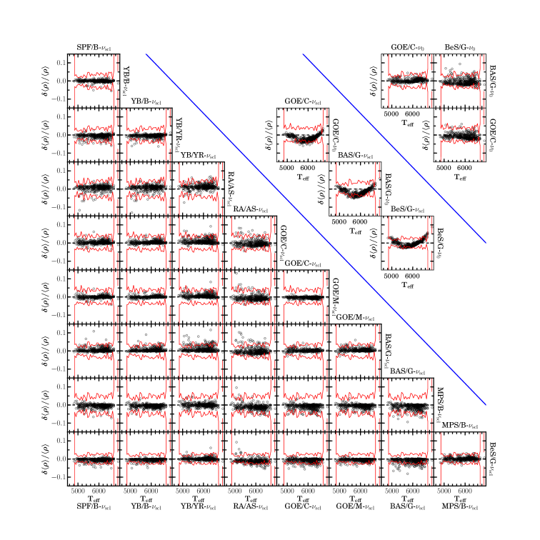
The general and most important lesson from these comparisons is that in the majority of cases the differences in the central values returned by the different GBMs are in agreement within the formal uncertainties returned by the pipelines, even for the modest 67 K $T_{\rm eff}$ uncertainty characteristic of the SDSS $T_{\rm eff}$ scale. This justifies the choice made in the determination of systematic uncertainties, in particular that central values returned by GBMs that are away by more than 3 times the standard deviations from the median value are considered outliers and removed from the sample used to determine the final systematic uncertainty (Sect. 4.4). The most clear examples of these outliers can be seen, for example, in comparisons involving RA/AS or MPS/B. But plots also show that out of the total number of stars and stellar parameters, the fractional number of results that are rejected is small.

Figure 22: Same as Fig. 21 but for stellar radius $R$. GBM labels are given in Table 1.

Focusing on the first group of comparisons, there are specific sets of GBM results that help to understand the impact of using different sets of evolutionary tracks/isochrones with the same statistical inference tool or vice versa. Our discussion here extends the one presented by C14. SFP/B, YB/B, and MPS/B rely on the same set of isochrones, so the differences among them should be related (mostly) to differences in the statistical methodology. In fact, the SFP/B vs YB/B typically shows very good agreement for all seismic quantities, with some of the smallest dispersions. On the other hand, when MPS/B is compared against them, the dispersion is somewhat larger, particularly for $M$ and $\tau$. Similarly, BAS/G and BeS/G results agree well. It has to be noticed in this case that, although the same evolutionary code has been used, the sets of models have been computed independently with somewhat different assumptions (see Table 8). Results for $\langle\rho\rangle$ in particular show that the presence of systematic differences between GBM results is not uncommon, because in many cases differences between pipelines show a preferential sign difference with most results for a given comparison been either positive or negative. The effect is typically small compared to statistical uncertainties, and it is beyond our scope here to go into the reasons why it occurs. We remark, however, that our procedure to estimate systematic uncertainties accounts for it. For other quantities this systematic difference between GBMs is smeared out because $T_{\rm eff}$ uncertainties play a more dominant role and scatter around the results.

Figure 23: Same as Fig. 21 but for stellar mass $M$. GBM labels are given in Table 1.

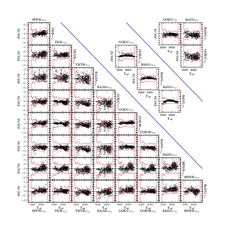
The comparison of GOE/C vs GOE/M and YB/B vs YB/YR are a measure of the impact of using different sets of stellar models with the same statistical inference. In fact, GOE/C and GOE/M compare very well with each other for all quantities, with typically the smallest dispersion even for stellar ages. For YB/B and YB/YR the comparison does not yield any remarkable results, with dispersions that are comparable to most other GBM comparisons. The latter case has been discussed more in extent in Sect. 4.3.1.

Overall, it does seem that using different sets of evolutionary tracks or different statistical inference tools yields similar dispersions on the results. In both cases, as stated above, differences are typically within the median formal uncertainties, which is a good sanity check of systematic uncertainties.

Figure 24: Same as Fig. 21 but for stellar age $\tau$. GBM labels are given in Table 1.

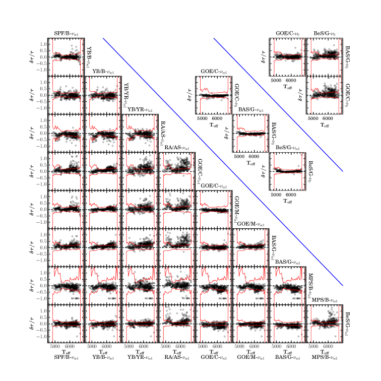
Results in the second group directly reflect differences induced by using the more physically accurate $\Delta\nu_{0}$ instead of $\Delta\nu_{\rm scl}$, as this is the only difference in the results within each subplot. Differences are shown here in the sense $G(\Delta\nu_{0})-G(\Delta\nu_{\rm scl})$, where G denotes any of the three GBMs included here. The effect of using $\Delta\nu_{0}$ is more clearly seen in $\langle\rho\rangle$, where as expected the trend reflects that shown in Fig. 4 but with the opposite sign and about twice as large in amplitude. There is a systematic offset between results based on BeS/G and those based on GOE/C and BAS/G. The reason is that in BeSPP, the grids of models are always rescaled such that a solar model in the grid reproduces $\Delta\nu_{\odot}$ and $\nu_{\rm max,\odot}$, even when $\Delta\nu_{0}$ is used. GOE/C-$\Delta\nu_{0}$ and BAS/G-$\Delta\nu_{0}$, on the other hand, do not include this additional scaling, leading to the larger systematic offset seen at the solar $T_{\rm eff}$. Aside from this scaling, the overall changes are the same for the three GBMs, which is reassuring that differences between $\Delta\nu_{0}$ and $\Delta\nu_{\rm scl}$ in stellar models are quite independent of the stellar models. The impact of using $\Delta\nu_{0}$ or $\Delta\nu_{\rm scl}$ also affects all other quantities, but in comparison to the formal uncertainties, it has a decreasing impact from $R$ to $\log{g}$, $M$ and $\tau$.

The final set of comparisons includes the combinations of GOE/C-$\Delta\nu_{0}$, BAS/G-$\Delta\nu_{0}$, and BeS/G-$\Delta\nu_{0}$. The dispersion between the first two is very similar to that between GOE/C and BASTA/G in the first group (based on $\Delta\nu_{\rm scl}$). Comparisons with BeS/G-$\Delta\nu_{0}$ show however larger dispersions. This is due to the additional scaling performed in BeS/G-$\Delta\nu_{0}$ and discussed in the previous paragraph, that puts results from this GBM aside. Recommended values in the catalog, however, are nevertheless based on BeS/G-$\Delta\nu_{0}$ for reasons explained in Sect. 4.1.

References

- Adelberger et al. (1998) Adelberger, E. G., Austin, S. M., Bahcall, J. N., et al. 1998, Reviews of Modern Physics, 70, 1265
- Adelberger et al. (2011) Adelberger, E. G., García, A., Robertson, R. G. H., et al. 2011, Reviews of Modern Physics, 83, 195
- Ahn et al. (2014) Ahn, C. P., Alexandroff, R., Allende Prieto, C., et al. 2014, ApJS, 211, 17
- Albareti et al. (2016) Albareti, F. D., Allende Prieto, C., et al. 2016, ArXiv e-prints, arXiv:1608.02013
- Alexander & Ferguson (1994) Alexander, D. R., & Ferguson, J. W. 1994, ApJ, 437, 879
- Allende Prieto et al. (2006) Allende Prieto, C., Beers, T. C., Wilhelm, R., et al. 2006, ApJ, 636, 804
- Anders et al. (2017) Anders, F., Chiappini, C., Rodrigues, T. S., et al. 2017, A&A, 597, A30
- Angulo et al. (1999) Angulo, C., Arnould, M., Rayet, M., et al. 1999, Nuclear Physics A, 656, 3
- Appourchaux et al. (2012) Appourchaux, T., Chaplin, W. J., García, R. A., et al. 2012, A&A, 543, A54
- Bahcall et al. (1995) Bahcall, J. N., Pinsonneault, M. H., & Wasserburg, G. J. 1995, Reviews of Modern Physics, 67, 781
- Ball et al. (2016) Ball, W. H., Beeck, B., Cameron, R. H., & Gizon, L. 2016, A&A, 592, A159
- Ball & Gizon (2014) Ball, W. H., & Gizon, L. 2014, A&A, 568, A123
- Bastien et al. (2013) Bastien, F. A., Stassun, K. G., Basri, G., & Pepper, J. 2013, Nature, 500, 427
- Bastien et al. (2016) —. 2016, ApJ, 818, 43
- Basu et al. (2010) Basu, S., Chaplin, W. J., & Elsworth, Y. 2010, ApJ, 710, 1596
- Bedding et al. (2010) Bedding, T. R., Huber, D., Stello, D., et al. 2010, ApJ, 713, L176
- Belkacem et al. (2011) Belkacem, K., Goupil, M. J., Dupret, M. A., et al. 2011, A&A, 530, A142
- Belkacem et al. (2013) Belkacem, K., Samadi, R., Mosser, B., Goupil, M.-J., & Ludwig, H.-G. 2013, in Astronomical Society of the Pacific Conference Series, Vol. 479, Progress in Physics of the Sun and Stars: A New Era in Helio- and Asteroseismology, ed. H. Shibahashi & A. E. Lynas-Gray, 61
- Bellinger et al. (2016) Bellinger, E. P., Angelou, G. C., Hekker, S., et al. 2016, ApJ, 830, 31
- Böhm-Vitense (1958) Böhm-Vitense, E. 1958, ZAp, 46, 108
- Boyajian et al. (2013) Boyajian, T. S., von Braun, K., van Belle, G., et al. 2013, ApJ, 771, 40
- Brown (1991) Brown, T. M. 1991, ApJ, 371, 396
- Bruntt et al. (2012) Bruntt, H., Basu, S., Smalley, B., et al. 2012, MNRAS, 423, 122
- Buchhave & Latham (2015) Buchhave, L. A., & Latham, D. W. 2015, ApJ, 808, 187
- Canuto et al. (1996) Canuto, V. M., Goldman, I., & Mazzitelli, I. 1996, ApJ, 473, 550
- Casagrande et al. (2010) Casagrande, L., Ramírez, I., Meléndez, J., Bessell, M., & Asplund, M. 2010, A&A, 512, A54
- Casagrande et al. (2014) Casagrande, L., Silva Aguirre, V., Stello, D., et al. 2014, ApJ, 787, 110
- Casagrande et al. (2016) Casagrande, L., Silva Aguirre, V., Schlesinger, K. J., et al. 2016, MNRAS, 455, 987
- Cassisi et al. (2003) Cassisi, S., Salaris, M., & Irwin, A. W. 2003, ApJ, 588, 862
- Chaplin et al. (2010) Chaplin, W. J., Appourchaux, T., Elsworth, Y., et al. 2010, ApJ, 713, L169
- Chaplin et al. (2011a) Chaplin, W. J., Kjeldsen, H., Christensen-Dalsgaard, J., et al. 2011a, Science, 332, 213
- Chaplin et al. (2011b) Chaplin, W. J., Bedding, T. R., Bonanno, A., et al. 2011b, ApJ, 732, L5
- Chaplin et al. (2014) Chaplin, W. J., Basu, S., Huber, D., et al. 2014, ApJS, 210, 1
- Chiappini et al. (2015) Chiappini, C., Anders, F., Rodrigues, T. S., et al. 2015, A&A, 576, L12
- Christensen-Dalsgaard (2008) Christensen-Dalsgaard, J. 2008, Ap&SS, 316, 13
- Christensen-Dalsgaard et al. (1996) Christensen-Dalsgaard, J., Dappen, W., Ajukov, S. V., et al. 1996, Science, 272, 1286
- Coelho et al. (2015) Coelho, H. R., Chaplin, W. J., Basu, S., et al. 2015, MNRAS, 451, 3011
- Corsaro et al. (2017) Corsaro, E., Mathur, S., García, R. A., et al. 2017, ArXiv e-prints, arXiv:1707.07474
- Creevey et al. (2017) Creevey, O. L., Metcalfe, T. S., Schultheis, M., et al. 2017, A&A, 601, A67
- Davies & Miglio (2016a) Davies, G. R., & Miglio, A. 2016a, ArXiv e-prints, arXiv:1601.02802
- Davies & Miglio (2016b) —. 2016b, Astronomische Nachrichten, 337, 774
- Davies et al. (2016) Davies, G. R., Silva Aguirre, V., Bedding, T. R., et al. 2016, MNRAS, 456, 2183
- Davies et al. (2017) Davies, G. R., Lund, M. N., Miglio, A., et al. 2017, A&A, 598, L4
- De Ridder et al. (2009) De Ridder, J., Barban, C., Baudin, F., et al. 2009, Nature, 459, 398
- De Silva et al. (2015) De Silva, G. M., Freeman, K. C., Bland-Hawthorn, J., et al. 2015, MNRAS, 449, 2604
- Delahaye & Pinsonneault (2006) Delahaye, F., & Pinsonneault, M. H. 2006, ApJ, 649, 529
- Demarque et al. (2008) Demarque, P., Guenther, D. B., Li, L. H., Mazumdar, A., & Straka, C. W. 2008, Ap&SS, 316, 31
- Edvardsson et al. (1993) Edvardsson, B., Andersen, J., Gustafsson, B., et al. 1993, A&A, 275, 101
- Eggleton et al. (1973) Eggleton, P. P., Faulkner, J., & Flannery, B. P. 1973, A&A, 23, 325
- Eisenstein et al. (2011) Eisenstein, D. J., Weinberg, D. H., Agol, E., et al. 2011, AJ, 142, 72
- Ferguson et al. (2005) Ferguson, J. W., Alexander, D. R., Allard, F., et al. 2005, ApJ, 623, 585
- Formicola et al. (2004) Formicola, A., Imbriani, G., Costantini, H., et al. 2004, Physics Letters B, 591, 61
- Freytag et al. (1996) Freytag, B., Ludwig, H.-G., & Steffen, M. 1996, A&A, 313, 497
- Gai et al. (2011) Gai, N., Basu, S., Chaplin, W. J., & Elsworth, Y. 2011, ApJ, 730, 63
- García et al. (2010) García, R. A., Mathur, S., Salabert, D., et al. 2010, Science, 329, 1032
- García et al. (2011) García, R. A., Hekker, S., Stello, D., et al. 2011, MNRAS, 414, L6
- García Pérez et al. (2016) García Pérez, A. E., Allende Prieto, C., Holtzman, J. A., et al. 2016, AJ, 151, 144
- Gaulme et al. (2014) Gaulme, P., Jackiewicz, J., Appourchaux, T., & Mosser, B. 2014, ApJ, 785, 5
- Gilliland et al. (2010) Gilliland, R. L., Brown, T. M., Christensen-Dalsgaard, J., et al. 2010, PASP, 122, 131
- González Hernández & Bonifacio (2009) González Hernández, J. I., & Bonifacio, P. 2009, A&A, 497, 497
- Gruyters et al. (2014) Gruyters, P., Nordlander, T., & Korn, A. J. 2014, A&A, 567, A72
- Gruyters et al. (2016) Gruyters, P., Lind, K., Richard, O., et al. 2016, A&A, 589, A61
- Gunn et al. (2006) Gunn, J. E., Siegmund, W. A., Mannery, E. J., et al. 2006, AJ, 131, 2332
- Handberg & Lund (2014) Handberg, R., & Lund, M. N. 2014, MNRAS, 445, 2698
- Harvey (1985) Harvey, J. 1985, in ESA Special Publication, Vol. 235, Future Missions in Solar, Heliospheric & Space Plasma Physics, ed. E. Rolfe & B. Battrick
- Heiter et al. (2015) Heiter, U., Jofré, P., Gustafsson, B., et al. 2015, A&A, 582, A49
- Hekker & Ball (2014) Hekker, S., & Ball, W. H. 2014, A&A, 564, A105
- Hekker et al. (2010) Hekker, S., Broomhall, A.-M., Chaplin, W. J., et al. 2010, MNRAS, 402, 2049
- Hekker et al. (2011) Hekker, S., Elsworth, Y., De Ridder, J., et al. 2011, A&A, 525, A131
- Holtzman et al. (2015) Holtzman, J. A., Shetrone, M., Johnson, J. A., et al. 2015, AJ, 150, 148
- Howell et al. (2014) Howell, S. B., Sobeck, C., Haas, M., et al. 2014, PASP, 126, 398
- Huber et al. (2009) Huber, D., Stello, D., Bedding, T. R., et al. 2009, Communications in Asteroseismology, 160, 74
- Huber et al. (2017) Huber, D., Zinn, J., Pinsonneault, M., Stello, D., & et al. 2017, in prep.
- Huber et al. (2011) Huber, D., Bedding, T. R., Stello, D., et al. 2011, ApJ, 743, 143
- Huber et al. (2012) Huber, D., Ireland, M. J., Bedding, T. R., et al. 2012, ApJ, 760, 32
- Huber et al. (2014) Huber, D., Silva Aguirre, V., Matthews, J. M., et al. 2014, ApJS, 211, 2
- Iglesias & Rogers (1996) Iglesias, C. A., & Rogers, F. J. 1996, ApJ, 464, 943
- Jacobson et al. (2011) Jacobson, H. R., Pilachowski, C. A., & Friel, E. D. 2011, AJ, 142, 59
- Kallinger et al. (2010) Kallinger, T., Mosser, B., Hekker, S., et al. 2010, A&A, 522, A1
- Kallinger et al. (2012) Kallinger, T., Hekker, S., Mosser, B., et al. 2012, A&A, 541, A51
- Kiefer et al. (2017) Kiefer, R., Schad, A., Davies, G., & Roth, M. 2017, A&A, 598, A77
- Kippenhahn & Weigert (1990) Kippenhahn, R., & Weigert, A. 1990, Stellar Structure and Evolution, 192
- Kjeldsen & Bedding (1995) Kjeldsen, H., & Bedding, T. R. 1995, A&A, 293, 87
- Kjeldsen & Bedding (2011) —. 2011, A&A, 529, L8
- Kurucz (1991) Kurucz, R. L. 1991, in NATO Advanced Science Institutes (ASI) Series C, Vol. 341, NATO Advanced Science Institutes (ASI) Series C, ed. L. Crivellari, I. Hubeny, & D. G. Hummer, 441
- Lebreton & Goupil (2014) Lebreton, Y., & Goupil, M. J. 2014, A&A, 569, A21
- Lebreton et al. (2008) Lebreton, Y., Montalbán, J., Christensen-Dalsgaard, J., Roxburgh, I. W., & Weiss, A. 2008, Ap&SS, 316, 187
- Lund et al. (2016) Lund, M. N., Chaplin, W. J., Casagrande, L., et al. 2016, PASP, 128, 124204
- Lund et al. (2017) Lund, M. N., Silva Aguirre, V., Davies, G. R., et al. 2017, ApJ, 835, 172
- Magic et al. (2010) Magic, Z., Serenelli, A., Weiss, A., & Chaboyer, B. 2010, ApJ, 718, 1378
- Majewski et al. (2015) Majewski, S. R., Schiavon, R. P., Frinchaboy, P. M., et al. 2015, ArXiv e-prints, arXiv:1509.05420
- Marconi et al. (2008) Marconi, M., Degl’Innocenti, S., Prada Moroni, P. G., & Ruoppo, A. 2008, Ap&SS, 316, 215
- Marques et al. (2013) Marques, J. P., Goupil, M. J., Lebreton, Y., et al. 2013, A&A, 549, A74
- Marta et al. (2008) Marta, M., Formicola, A., Gyürky, G., et al. 2008, Phys. Rev. C, 78, 022802
- Mathur et al. (2016) Mathur, S., García, R. A., Huber, D., et al. 2016, ApJ, 827, 50
- Mathur et al. (2010) Mathur, S., García, R. A., Régulo, C., et al. 2010, A&A, 511, A46
- Mathur et al. (2012) Mathur, S., Hekker, S., Trampedach, R., et al. 2012, in Astronomical Society of the Pacific Conference Series, Vol. 462, Progress in Solar/Stellar Physics with Helio- and Asteroseismology, ed. H. Shibahashi, M. Takata, & A. E. Lynas-Gray, 375
- Mészáros et al. (2013) Mészáros, S., Holtzman, J., García Pérez, A. E., et al. 2013, AJ, 146, 133
- Metcalfe et al. (2014) Metcalfe, T. S., Creevey, O. L., Doğan, G., et al. 2014, ApJS, 214, 27
- Michel et al. (2008) Michel, E., Baglin, A., Auvergne, M., et al. 2008, Science, 322, 558
- Morel & Lebreton (2008) Morel, P., & Lebreton, Y. 2008, Ap&SS, 316, 61
- Mosser & Appourchaux (2009) Mosser, B., & Appourchaux, T. 2009, A&A, 508, 877
- Mosser et al. (2012) Mosser, B., Elsworth, Y., Hekker, S., et al. 2012, A&A, 537, A30
- Mosser et al. (2013) Mosser, B., Michel, E., Belkacem, K., et al. 2013, A&A, 550, A126
- Nidever et al. (2015) Nidever, D. L., Holtzman, J. A., Allende Prieto, C., et al. 2015, AJ, 150, 173
- Nordlander et al. (2012) Nordlander, T., Korn, A. J., Richard, O., & Lind, K. 2012, ApJ, 753, 48
- Nordström et al. (2004) Nordström, B., Mayor, M., Andersen, J., et al. 2004, A&A, 418, 989
- Önehag et al. (2014) Önehag, A., Gustafsson, B., & Korn, A. 2014, A&A, 562, A102
- Paxton et al. (2013) Paxton, B., Cantiello, M., Arras, P., et al. 2013, ApJS, 208, 4
- Pietrinferni et al. (2004) Pietrinferni, A., Cassisi, S., Salaris, M., & Castelli, F. 2004, ApJ, 612, 168
- Pinsonneault et al. (2012) Pinsonneault, M. H., An, D., Molenda-Żakowicz, J., et al. 2012, ApJS, 199, 30
- Pinsonneault et al. (2014) Pinsonneault, M. H., Elsworth, Y., Epstein, C., et al. 2014, ApJS, 215, 19
- Quirion et al. (2010) Quirion, P.-O., Christensen-Dalsgaard, J., & Arentoft, T. 2010, ApJ, 725, 2176
- Richard et al. (2002) Richard, O., Michaud, G., Richer, J., et al. 2002, ApJ, 568, 979
- Rogers & Nayfonov (2002) Rogers, F. J., & Nayfonov, A. 2002, ApJ, 576, 1064
- Rosenthal et al. (1999) Rosenthal, C. S., Christensen-Dalsgaard, J., Nordlund, Å., Stein, R. F., & Trampedach, R. 1999, A&A, 351, 689
- Roxburgh (2017) Roxburgh, I. W. 2017, A&A, 604, A42
- Salaris & Cassisi (2008) Salaris, M., & Cassisi, S. 2008, A&A, 487, 1075
- Samadi (2011) Samadi, R. 2011, in Lecture Notes in Physics, Berlin Springer Verlag, Vol. 832, Lecture Notes in Physics, Berlin Springer Verlag, ed. J.-P. Rozelot & C. Neiner, 305
- Sandquist (2004) Sandquist, E. L. 2004, MNRAS, 347, 101
- Serenelli et al. (2013) Serenelli, A. M., Bergemann, M., Ruchti, G., & Casagrande, L. 2013, MNRAS, 429, 3645
- Serenelli & Fukugita (2007) Serenelli, A. M., & Fukugita, M. 2007, ApJS, 172, 649
- Silva Aguirre et al. (2011) Silva Aguirre, V., Chaplin, W. J., Ballot, J., et al. 2011, ApJ, 740, L2
- Silva Aguirre et al. (2012) Silva Aguirre, V., Casagrande, L., Basu, S., et al. 2012, ApJ, 757, 99
- Silva Aguirre et al. (2015) Silva Aguirre, V., Davies, G. R., Basu, S., et al. 2015, MNRAS, 452, 2127
- Silva Aguirre et al. (2017) Silva Aguirre, V., Lund, M. N., Antia, H. M., et al. 2017, ApJ, 835, 173
- Sonoi et al. (2015) Sonoi, T., Samadi, R., Belkacem, K., et al. 2015, A&A, 583, A112
- Stancliffe et al. (2016) Stancliffe, R. J., Fossati, L., Passy, J.-C., & Schneider, F. R. N. 2016, A&A, 586, A119
- Stassun & Torres (2016) Stassun, K. G., & Torres, G. 2016, ApJ, 831, L6
- Stello et al. (2009a) Stello, D., Chaplin, W. J., Basu, S., Elsworth, Y., & Bedding, T. R. 2009a, MNRAS, 400, L80
- Stello et al. (2009b) Stello, D., Chaplin, W. J., Bruntt, H., et al. 2009b, ApJ, 700, 1589
- Stello et al. (2017) Stello, D., Zinn, J., Elsworth, Y., et al. 2017, ApJ, 835, 83
- Tayar et al. (2015) Tayar, J., Ceillier, T., García-Hernández, D. A., et al. 2015, ApJ, 807, 82
- Taylor (2007) Taylor, B. J. 2007, AJ, 133, 370
- Thoul et al. (1994) Thoul, A. A., Bahcall, J. N., & Loeb, A. 1994, ApJ, 421, 828
- Trampedach et al. (2017) Trampedach, R., Aarslev, M. J., Houdek, G., et al. 2017, MNRAS, 466, L43
- Ulrich (1986) Ulrich, R. K. 1986, ApJ, 306, L37
- Valentini et al. (2017) Valentini, M., Chiappini, C., Davies, G. R., et al. 2017, A&A, 600, A66
- van Saders & Pinsonneault (2013) van Saders, J. L., & Pinsonneault, M. H. 2013, ApJ, 776, 67
- VandenBerg et al. (2012) VandenBerg, D. A., Bergbusch, P. A., Dotter, A., et al. 2012, ApJ, 755, 15
- Verner et al. (2011) Verner, G. A., Elsworth, Y., Chaplin, W. J., et al. 2011, MNRAS, 415, 3539
- Villante et al. (2014) Villante, F. L., Serenelli, A. M., Delahaye, F., & Pinsonneault, M. H. 2014, ApJ, 787, 13
- Weiss & Schlattl (2008) Weiss, A., & Schlattl, H. 2008, Ap&SS, 316, 99
- White et al. (2011) White, T. R., Bedding, T. R., Stello, D., et al. 2011, ApJ, 743, 161
- White et al. (2013) White, T. R., Huber, D., Maestro, V., et al. 2013, MNRAS, 433, 1262
- Wilson et al. (2012) Wilson, J. C., Hearty, F., Skrutskie, M. F., et al. 2012, in Proc. SPIE, Vol. 8446, Ground-based and Airborne Instrumentation for Astronomy IV, 84460H
- Zamora et al. (2015) Zamora, O., García-Hernández, D. A., Allende Prieto, C., et al. 2015, AJ, 149, 181
- Zasowski et al. (2013) Zasowski, G., Johnson, J. A., Frinchaboy, P. M., et al. 2013, AJ, 146, 81
- Zhao et al. (2012) Zhao, G., Zhao, Y.-H., Chu, Y.-Q., Jing, Y.-P., & Deng, L.-C. 2012, Research in Astronomy and Astrophysics, 12, 723