$\eta$ and $\eta^{\prime}$ masses and decay constants

Abstract

We present preliminary results for the masses and decay constants of the $\eta$ and $\eta^{\prime}$ mesons using CLS $N_{f}=2+1$ ensembles.

One of the major challenges in these calculations are the large statistical fluctuations due to disconnected quark loops. We tackle these by employing a combination of noise reduction techniques which are tuned to minimize the statistical error at a fixed cost.

On the analysis side we carefully assess excited states contributions by using a direct fit approach.

1 Introduction

The $\eta$ and $\eta^{\prime}$ play an important role in many QCD processes and are directly connected to the chiral anomaly of QCD. Their electromagnetic transition form factors are of great phenomenological interest and have been studied theoretically, e.g., using light cone sum rules Agaev:2014wna . However, little is known about their wavefunctions and the quark mass dependence of singlet-octet mixing and first-principles determinations are needed. On the lattice, the $\eta$ and $\eta^{\prime}$ mesons are difficult to study. Nonetheless, quite some progress has been made, e.g., in Kuramashi:1994aj ; Struckmann:2000bt ; McNeile:2000hf ; Lesk:2002gd ; Christ:2010dd ; Dudek:2011tt ; Gregory:2011sg ; Michael:2013vba ; Bali:2014pva .

The fact that the $\eta$ and $\eta^{\prime}$ states are not flavour eigenstates presents a challenge. The mass eigenstates are mixtures of flavour singlet and octet states, i.e.,

$$\mid\eta\rangle=\cos\theta\mid\eta_{8}\rangle-\sin\theta\mid\eta_{1}\rangle\text{,}\qquad\mid\eta^{\prime}\rangle=\sin\theta^{\prime}\mid\eta_{8}\rangle+\cos\theta^{\prime}\mid\eta_{1}\rangle\text{,}$$ (1)

where the angles $\theta$ and $\theta^{\prime}$ will in general depend on the choice of $\mid\eta_{1}\rangle$ and $\mid\eta_{8}\rangle$, e.g., on the scale and the smearing applied.

This can also be expressed in matrix form,

$$\begin{pmatrix}\mathcal{C}_{\eta}&0\\ 0&\mathcal{C}_{\eta^{\prime}}\end{pmatrix}=U\begin{pmatrix}\mathcal{C}_{88}&\mathcal{C}_{81}\\ \mathcal{C}_{18}&\mathcal{C}_{11}\end{pmatrix}U^{T}\text{, where}\quad\mathcal{C}_{ij}=\langle P_{i}(x)\mid P_{j}(y)\rangle\text{,}\quad\text{and}\quad U(\theta,\theta^{\prime})=\begin{pmatrix}\cos\theta&-\sin\theta\\ \sin\theta^{\prime}&\phantom{-}\cos\theta^{\prime}\end{pmatrix}$$ (2)

is a non-unitary rotation matrix to allow for possible gluonic and other excited states contributions. $\mathcal{C}_{ij}$ with $i,j\in\{8,1\}$ are correlators connecting pseudoscalar octet and singlet operators, respectively:

$$P_{8}=\frac{1}{\sqrt{6}}\left(\bar{u}\gamma_{5}u+\bar{d}\gamma_{5}d-2\bar{s}\gamma_{5}s\right)\quad\text{and}\quad P_{1}=\frac{1}{\sqrt{3}}\left(\bar{u}\gamma_{5}u+\bar{d}\gamma_{5}d+\bar{s}\gamma_{5}s\right)\text{.}$$ (3)

When performing the Wick contractions for the matrix elements $\mathcal{C}_{ij}$, another difficulty emerges: disconnected loops appear which are inherently noisy and expensive to compute on the lattice. Efficient solvers for the Dirac equation and noise reduction techniques are mandatory to obtain decent signals.

In these proceedings we attempt a determination of the masses and leading distribution amplitudes of the $\eta$ and $\eta^{\prime}$ mesons, refining our techniques on two of the many existing $N_{f}=2+1$ CLS ensembles Bruno:2014jqa with non-perturbatively improved Wilson fermions at $\beta=3.4$, corresponding to a lattice spacing $a\approx 0.0864\,\mathrm{fm}$ (determined using $\sqrt{8\,t_{0}}=0.415\,\mathrm{fm}$ Bruno:2016plf ). The first of the two, ensemble U103, is at the $N_{f}=3$ symmetric point with $m_{\pi}=m_{K}\approx 415\,\textrm{MeV}$. The other, H105, is along the same line of constant average quark mass, with $m_{\pi}\approx 287\,\textrm{MeV}$ and $m_{K}\approx 487\,\textrm{MeV}$.

2 Computation of disconnected loops

The entries $\mathcal{C}_{ij}$ of the matrix in Eq. (2) are given by

$$\mathcal{C}_{88}= \frac{1}{3}\left(C_{\ell\bar{\ell}}+2C_{s\bar{s}}-2D_{\ell\bar{\ell}}+2D_{\ell\bar{s}}+2D_{s\bar{\ell}}-2D_{s\bar{s}}\right)$$ (4)

$$\mathcal{C}_{18}=\mathcal{C}_{81}= \frac{\sqrt{2}}{3}\left(C_{\ell\bar{\ell}}-C_{s\bar{s}}-2D_{\ell\bar{\ell}}+2D_{\ell\bar{s}}-D_{s\bar{\ell}}+D_{s\bar{s}}\right)$$ (5)

$$\mathcal{C}_{11}= \frac{1}{3}\left(2C_{\ell\bar{\ell}}+C_{s\bar{s}}-4D_{\ell\bar{\ell}}-2D_{\ell\bar{s}}-2D_{s\bar{\ell}}-D_{s\bar{s}}\right)\text{,}$$ (6)

and are linear combinations of connected and disconnected pseudoscalar correlators,

$$C^{P}_{f\bar{f}}(\delta t)=\operatorname{tr}\left(\gamma_{5}S^{-1}_{f}(\delta t)\gamma_{5}S^{-1}_{f}(0)\right)\text{,}$$ (7)

$$D^{P}_{f\bar{g}}(\delta t)=\operatorname{tr}\left(\gamma_{5}S^{-1}_{f}(\delta t)\right)\operatorname{tr}\left(\gamma_{5}S^{-1}_{g}(0)\right)\text{,}$$ (8)

with light and strange quark flavours $f,g\in\{\ell,s\}$ and $S^{-1}_{f}$ being the quark propagator of flavour $f$. While the connected correlators can be cheaply computed by exploiting the $\gamma_{5}\text{-hermiticity}$ of the Dirac operator (we use one point source per configuration), the disconnected loops $L_{f}(t)=\operatorname{tr}\gamma_{5}S^{-1}_{f}(t)$ must be estimated stochastically. We do so by inverting the Dirac equation on time-diluted $\mathbb{Z}_{2}\otimes i\mathbb{Z}_{2}$ sources, where a distance of $4a$ between non-zero time slices was found to be optimal. Additionally, we employ the hopping parameter expansion to improve the signal-to-noise ratio of the loops by exploiting $L_{f}(t)=\operatorname{tr}\Gamma S^{-1}_{f}(t)=\kappa_{f}^{k}\operatorname{tr}\Gamma D^{k}S^{-1}_{f}(t)$, where $D$ here is the hopping part in the Dirac operator $S_{f}=\mathds{1}+\kappa_{f}D$ and $k=2$ for $\Gamma=\gamma_{5}$ and $k=4$ for $\Gamma=\gamma_{\mu}\gamma_{5}$ are the maximum number of applications that can be used for our action. See Bali:2009hu and references therein for more details on these noise reduction techniques.

It turned out that 96 stochastic estimates for each quark flavour and time dilution are also sufficient to obtain reasonable signals for the axialvector loop, that is needed for the extraction of the decay constants. When performing this many solves per configuration, it is crucial to employ a modern solver. We use a multigrid solver that has been optimized specifically for the KNL architecture qp3 .

3 Extraction of physical states

At the $N_{f}=3$ flavour symmetric point where $S^{-1}_{\ell}=S^{-1}_{s}$ the elements of the correlator matrix, Eqs. (4) to (6), simplify leading to a diagonal matrix: In this limit, the $\eta$ is a pure octet state and equal in mass to the pion, whereas the $\eta^{\prime}$ is entirely a singlet:

$$\mathcal{C}_{88}(\delta t)= \mathcal{C}_{\eta}(\delta t)=\mathcal{C}_{\pi}(\delta t),$$ (9)

$$\mathcal{C}_{11}(\delta t)= \mathcal{C}_{\eta^{\prime}}(\delta t)=\mathcal{C}_{\pi}(\delta t)-3D(\delta t)\text{.}$$ (10)

For sufficiently large times, where excited states can be neglected, both the pion and the $\eta^{\prime}$ correlators are single-exponentials. Consequently, the disconnected correlator is a double-exponential

$$D(\delta t)=\frac{1}{3}\left(\mathcal{C}_{\pi}(\delta t)-\mathcal{C}_{\eta^{\prime}}(\delta t)\right)\to\frac{1}{3}\left(A_{\pi}\exp(-m_{\pi}\delta t)-A_{\eta^{\prime}}\exp(-m_{\eta^{\prime}}\delta t)\right)\text{,}$$ (11)

where $A_{\pi},A_{\eta^{\prime}}>0$. The (lighter) pion mass dominates at large times over the heavy $\eta^{\prime}$, which leaves only a small window for the extraction of the $\eta^{\prime}$ state: at very small times excited states impede the extraction of the ground state while at large time separations the relative error arising from the disconnected diagrams grows rapidly and makes resolving the small difference to the pion correlator impossible.

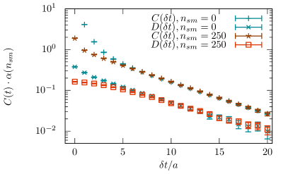
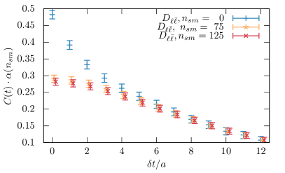
Figure 1: left: Pseudoscalar connected and disconnected correlators are shown, both for local sources and sinks ($n_{sm}=0$) and after $n_{sm}=125$ smearing iterations for U103. The correlators are scaled to match such that they agree at large times. With no smearing excited states are clearly visible both in the connected and the disconnected correlators. right: The same for the light-light disconnected correlator of H105. The smeared correlators do not exhibit significant excited states after $n_{sm}=75$ iterations.

We employ Wuppertal quark smearing Gusken:1989ad both to the source and the sink loops to enhance the ground over excited states. A small number of smearing iterations turned out to be sufficient to suppress excited states and achieve moderate errors in the final results. In particular for the disconnected correlators comparably few iterations seem to be sufficient, see Fig. 1.

The observations above are also valid away from the symmetric point. There, the correlator matrix, Eq. (2), must first be diagonalized to extract the physical states. This is usually done by solving the generalized eigenvalue problem, yielding the physical correlators as eigenvalues. However, we observed comparably large errors and unstable results when changing the parameters of the method. Instead, we insert Eqs. (4) – (6) into Eq. (2) and obtain a system of three linear equations that we solve for the three independent disconnected correlators, $D_{\ell\bar{\ell}},D_{\ell\bar{s}},\text{and}D_{s\bar{s}}$, yielding similar expressions as at the symmetric point, Eq. (11). In the $N_{f}=2+1$ case, the resulting formulae are more complex and depend on two angles $\theta$ and $\theta^{\prime}$, two connected correlators for the pion and the $s\bar{s}$, and the wanted $\eta$ and $\eta^{\prime}$ correlators. Plugging single-exponentials into the correlators, we end up with a total of ten independent parameters.

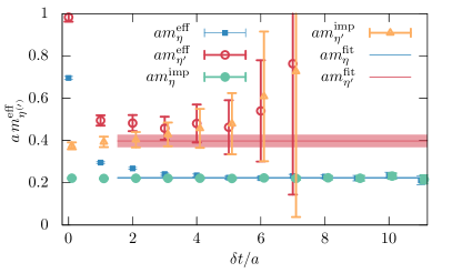
Figure 2: left: Combined fit to the disconnected correlators of H105, using information from a previous fit to the connected correlators. We obtain typical values of $\chi^{2}/\mathrm{d.o.f.}\approx 1$ in correlated fits. right: Effective masses for the $\eta$ and $\eta^{\prime}$, computed from their reconstructed correlators, denoted $a\,m^{\mathrm{eff}}_{\eta^{(\prime)}}$, and with the connected correlators replaced by their fitted curves ($a\,m^{\mathrm{imp}}_{\eta^{(\prime)}}$), along with the fitted mass values from the combined fit. Shaded regions represent the errors of the fitted masses and the fit range of the disconnected correlators. Connected correlators are fitted in the range $\delta t/a\in[15,40]$. Excited states arising from the connected correlators at earlier times are clearly visible.

We perform a combined fit to determine these parameters. The connected correlators naturally do not depend on the disconnected ones and can be fitted first, reducing the number of parameters to six. Being able to tune the fit ranges independently we can fit the connected correlators in a region where we are sure to be free of excited states contaminations whereas the disconnected fits can start at smaller times to capture the heavy $\eta^{\prime}$ state sufficiently well. At later times, the well determined connected correlators constrain the fit. This approach is similar in spirit to the subtraction method of Neff:2001zr ; Jansen:2008wv ; Michael:2013vba . Fig. 2 demonstrates that the fit describes the data points and the fit errors actually decrease at large times, confirming our expectations.

Note that in Eq. (2) we chose the octet-singlet basis, which is just one particular choice and we can as well work in any other basis, e.g., in the flavour basis, where

$$\mid\eta\rangle=\frac{1}{\sqrt{2}}\cos\vartheta\mid\bar{u}\gamma_{5}u+\bar{d}\gamma_{5}d\rangle-\sin\vartheta\mid\bar{s}\gamma_{5}s\rangle$$ (12)

$$\mid\eta^{\prime}\rangle=\frac{1}{\sqrt{2}}\sin\vartheta^{\prime}\mid\bar{u}\gamma_{5}u+\bar{d}\gamma_{5}d\rangle+\cos\vartheta^{\prime}\mid\bar{s}\gamma_{5}s\rangle\text{,}$$ (13)

with different angles $\vartheta^{(\prime)}$. In this case, the fit forms look a bit simpler but the resulting correlators and masses are (numerically) equal.

To remove any potential constant shifts from our (disconnected) correlators stemming from an incomplete sampling of the topological sectors, we also fit to

$$-\hat{\partial}_{4}\mathcal{C}(\delta t)\approx\frac{\mathcal{C}(\delta t-a)-\mathcal{C}(\delta t+a)}{2a}$$ (14)

as suggested in Feng:2009ij ; Umeda:2007hy . We found that this reduces the error and also stabilizes the result with respect to different fit ranges.

In order to further improve statistics in the mass estimates, and as a cross check on systematic errors we also combine data at finite momentum and fit to the dispersion relation

$$aE(m,p)=\sqrt{a^{2}m^{2}+a^{2}p^{2}}\text{,}$$ (15)

where $a^{2}p^{2}=\sum_{\mu}k^{2}_{\mu}\frac{4\pi^{2}}{L_{\mu}^{2}}$ is the square of the lattice momentum, $L_{\mu}$ is the number of lattice points in direction $\hat{\mu}$ and $-L_{\mu}/2\leq k_{\mu}<L_{\mu}/2$ are the integer momentum components.

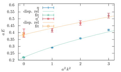
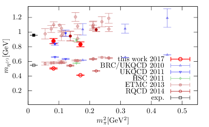
Figure 3: left: Fits to the dispersion relation, Eq. (15), combining data at several momenta. right: Summary plot of recent lattice determinations of the $\eta$ and $\eta^{\prime}$ masses, cf. Christ:2010dd ; Gregory:2011sg ; Dudek:2011tt ; Michael:2013vba .

From this fitting approach, we obtain for the U103 ensemble at the flavour symmetric point,

$$m_{\eta}=m_{\pi}=412(2)\,\mathrm{MeV},\quad m_{\eta^{\prime}}=833(33)\,\mathrm{MeV}\text{,}$$ (16)

and away from that point, for H105, at a pion mass of $282\,\mathrm{MeV}$,

$$m_{\eta}=504(7)\,\mathrm{MeV},\quad m_{\eta^{\prime}}=878(35)\,\mathrm{MeV}\text{.}$$ (17)

Fig. 3 compares these results with other lattice determinations and the physical point. It should be stressed that, like in the RQCD 2014 study Bali:2014pva , the two considered ensembles are on a line of constant average quark mass and approach the physical point on a different trajectory than other ($m_{s}\approx\mathrm{const.}$) studies.

4 Decay constants

Having extracted masses and the angles, we can construct the correlators

$$\mathcal{C}_{A^{i}\eta^{(\prime)}}(\delta t)=\langle 0\mid A^{i}_{\mu}(\delta t)\mid\eta^{(\prime)}\rangle\text{,}\quad\mathcal{C}_{P^{i}\eta^{(\prime)}}(\delta t)=\langle 0\mid P^{i}(\delta t)\mid\eta^{(\prime)}\rangle\rangle\text{,}\quad\mathcal{C}_{\eta^{(\prime)}\eta^{(\prime)}}(\delta t)=\langle\eta^{(\prime)}(\delta t)\mid\eta^{(\prime)}\rangle$$ (18)

where $P^{i}$ labels the octet ($i=8$) and singlet ($i=1$) pseudoscalar local currents, defined in Eq. (3) and $A^{i}_{\mu}$ similarly defines the axialvector currents. Using these correlators, one can compute decay constants which read

$$\langle 0\mid A_{\mu}^{i}\mid\eta^{(\prime)}(p)\rangle=if_{N}^{i}p_{\mu}\text{.}$$ (19)

This results in four different effective decay constants at momentum $p=0$,

$$f^{i,\mathrm{eff}}_{\eta^{(\prime)}}(\delta t)=Z_{A}^{i}\frac{\sqrt{2}\mathcal{C}_{A^{i}\eta^{(\prime)}}(\delta t)}{\sqrt{\mathcal{C}_{\eta^{(\prime)}\eta^{(\prime)}}(\delta t)m_{\eta^{(\prime)}}}}\exp(m_{\eta^{(\prime)}}\delta t/2)\text{,}$$ (20)

which are constant over some range in $\delta t$ where excited states can be neglected and the correlators have not yet vanished in the noise.

For (partial) $\mathcal{O}(a)$ improvement, we replace

$$\mathcal{C}_{A^{i}\eta^{(\prime)}}\to\tilde{\mathcal{C}}_{A^{i}\eta^{(\prime)}}=(1+b_{A}a\,m_{i})(\mathcal{C}_{A^{i}\eta^{(\prime)}}+ac_{A}\partial_{4}\mathcal{C}_{P^{i}\eta^{(\prime)}})\text{,}$$ (21)

where $a\,m_{8}=\frac{a}{3}(m_{l}+2\,m_{s})$ and $a\,m_{1}=\frac{a}{3}(2\,m_{l}+m_{s})$. We take the non-perturbatively determined improvement coefficients $b_{A}$ from Korcyl:2016ugy , $c_{A}$ from Bulava:2015bxa and $Z_{A}^{8}$ from Bulava:2016ktf . For the axial renormalization factor, the difference between $Z_{A}^{8}$ and $Z_{A}^{1}$ is of $\mathcal{O}(\alpha_{s}^{2})$ and known perturbatively Constantinou:2016ieh . For this lattice spacing and action it is at the level of 2 %, which is in line with preliminary recent non-perturbative estimates Bali:2017jyw . From these numbers, we estimate the systematic uncertainty from renormalization to be around 5 %. In this work, we take the non-perturbative octet renormalization factor together with the perturbative difference at a scale of $2\,\mathrm{GeV}$.

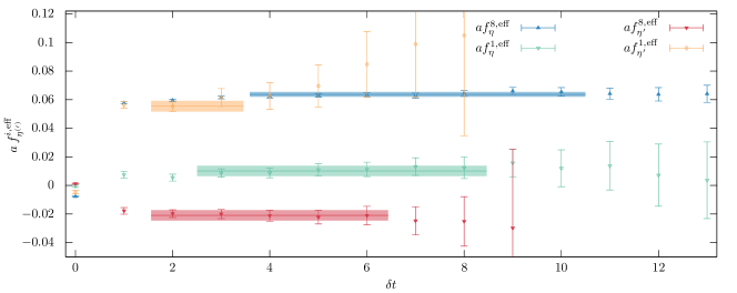
Figure 4: Effective decay constants as defined in Eq. (20) for H105. Shaded regions indicate fit ranges and errors.

As can be seen in Fig. 4, we face the "window problem" again: The axialvector loops are even noisier than the pseudoscalar ones so that the signal is lost very early in Euclidean time. Also, being local at the sink, we need to take special care of excited states. By fixing the masses to their previously determined values we can take weighted averages ("one-parameter fits") to each of the effective decay constants, tuning the ranges individually. The results are compatible with Bali:2014pva , however, $f_{\eta^{\prime}}^{1}$ is quite a bit larger, which might be due to insufficient treatment of excited states in that channel.

It is common to give the decay constants in the flavour basis, which we recover from the fitted values by taking the linear combinations at the scale of interest, $\mu=2\,\mathrm{GeV}$,

$$f_{\eta^{(\prime)}}^{l}=\sqrt{\frac{1}{3}}f_{\eta^{(\prime)}}^{8}+\sqrt{\frac{2}{3}}f_{\eta^{(\prime)}}^{1},\quad f_{\eta^{(\prime)}}^{s}=-\sqrt{\frac{2}{3}}f_{\eta^{(\prime)}}^{8}+\sqrt{\frac{1}{3}}f_{\eta^{(\prime)}}^{1}\text{.}$$ (22)

Usually, these are parameterized in terms of two constants and two angles,

$$\begin{pmatrix}f_{\eta}^{l}&f_{\eta}^{s}\\ f_{\eta^{\prime}}^{l}&f_{\eta^{\prime}}^{s}\end{pmatrix}=\begin{pmatrix}f_{l}\,\cos\theta_{l}&-f_{s}\,\sin\theta_{s}\\ f_{l}\,\sin\theta_{l}&f_{s}\,\cos\theta_{s}\end{pmatrix}=U^{T}(-\theta_{l},-\theta_{s})\begin{pmatrix}f^{l}&0\\ 0&f^{s}\end{pmatrix}\text{,}$$ (23)

which we extract simply via

$$\theta_{l}= \arctan\frac{f_{\eta^{\prime}}^{l}}{f_{\eta}^{l}}\text{,} \quad\theta_{s}= -\arctan\frac{f_{\eta}^{s}}{f_{\eta^{\prime}}^{s}}\text{,} f_{l}= \frac{f_{\eta}^{l}}{2\cos\theta_{l}}+\frac{f_{\eta^{\prime}}^{l}}{2\sin\theta_{l}}\text{,} \quad f_{s}= \frac{f_{\eta^{\prime}}^{s}}{2\cos\theta_{s}}-\frac{f_{\eta}^{s}}{2\sin\theta_{s}}\text{.}$$ (24)

Additionally, we monitor unitarity violations by considering the difference of the angles $\delta\theta=\theta_{l}-\theta_{s}$, which has a non-vanishing value if there is a gluonic contribution to $f_{\eta^{(\prime)}}^{i}$ and is related to the low-energy constant $\Lambda_{1}$ Feldmann:1999uf ,

$$f_{l}f_{s}\sin(\theta_{l}-\theta_{s})=\frac{\sqrt{2}}{3}f_{\pi}^{2}\Lambda_{1}\text{.}$$ (25)

For the two ensembles, we obtain for the decay constants

$$\text{U103:}\quad f_{l}/f_{\pi}= 1.20(7), \quad f_{s}/f_{\pi}= 1.27(2)\text{,}\qquad\text{H105:}\quad f_{l}/f_{\pi}= 1.27(7), \quad f_{s}/f_{\pi}= 1.39(5)\text{,}$$ (26)

and for the two angles and $\Lambda_{1}$

$$\text{U103:}\quad\theta_{l}= 61.3(1.8)\degree, \quad\theta_{s}= 65.4(1.6)\degree, \quad\delta\theta= -4.1(3.4)\degree, \quad\Lambda_{1}=-0.23(17)\text{,}$$ (27)

$$\text{H105:}\quad\theta_{l}= 59.7(1.6)\degree, \quad\theta_{s}= 66.9(1.3)\degree, \quad\delta\theta= -7.2(2.9)\degree, \quad\Lambda_{1}=-0.47(17)\text{,}$$ (28)

Within present statistics, we find $\theta_{l}\approx\theta_{s}$, i.e., we do not see any strong OZI violation, however, the difference increases at the H105 ensemble compared to the symmetric point. It will be interesting to see if this becomes stronger at smaller quark masses.

Compared to phenomenology, the light decay constants have rather large values:

$$\text{\cite[cite]{\@@bibref{Authors Phrase1YearPhrase2}{Feldmann:1998vh,Feldmann:1998sh}{\@@citephrase{(}}{\@@citephrase{)}}}}\quad f_{l}/f_{\pi}= 1.07(2), \quad f_{s}/f_{\pi}= 1.34(6)\text{,} \quad\theta_{l}=\theta_{s}=39.3(1.0)\text{,}$$ (29)

$$\text{\cite[cite]{\@@bibref{Authors Phrase1YearPhrase2}{Escribano:2005qq}{\@@citephrase{(}}{\@@citephrase{)}}}}\quad f_{l}/f_{\pi}= 1.09(3), \quad f_{s}/f_{\pi}= 1.66(6)\text{,} \quad\theta_{l}=\theta_{s}=40.7(1.4)\text{.}$$ (30)

As already mentioned, this might be due to underestimated excited states, in particular in the correlator $\mathcal{C}_{A^{i}\eta^{\prime}}^{1}$. Being local at the sink, the chosen smearing might be insufficient to completely remove them. It has also been shown Bruno:2016plf that cutoff effects are large, e.g., for the combination $\sqrt{8\,t_{0}}f_{\pi K}$ in particular at this lattice spacing. It remains to be seen how the values change when approaching the physical point, i.e., at finer lattices and smaller quark masses.

5 Summary

In these proceedings, we employed several noise reduction techniques to obtain disconnected loops at a precision that allows us to study the $\eta/\eta^{\prime}$ system on two CLS ensembles.

To extract the physical states, we directly fit to the correlators. This, in combination with quark smearing enables us to capture the small-t behaviour, encoding the $\eta^{\prime}$ physics and still have excited states under control. In a second fit we incorporate even noisier data from the axialvector channel to determine decay constants directly. The results are encouraging, however, a detailed analysis of systematic errors still remains to be done.

We plan to do so by analysing more CLS ensembles, following two distinct quark mass trajectories. The combination of ensembles along the line of constant average quark mass with ensembles where the strange quark mass is kept fixed, as well as going towards lighter masses will allow for a controlled chiral extrapolation. Also finite lattice spacing and volume effects will be investigated.

6 Acknowledgments

This work was supported by the DFG SFB/TRR 55. We thank our colleagues in CLS [http://wiki-zeuthen.desy.de/CLS/CLS] for the joint effort in the generation of the gauge field ensembles which form a basis for the here described computation. The authors gratefully acknowledge the Gauss Centre for Supercomputing (GCS) for providing computing time through the John von Neumann Institute for Computing (NIC) on the GCS share of the super-computer JUQUEEN at JÃlich Supercomputing Centre (JSC). GCS is the alliance of the three national supercomputing centers HLRS (UniversitÃt Stuttgart), JSC (Forschungszentrum JÃlich), and LRZ (Bayerische Akademie der Wissenschaften), funded by the German Federal Ministry of Education and Research (BMBF) and the German State Ministries for Research of Baden-WÃrttemberg (MWK), Bayern (StMWFK) and Nordrhein-Westfalen (MIWF).

References

• (1) S.S. Agaev, V.M. Braun, N. Offen, F.A. Porkert, A. SchÃfer, Phys. Rev. D90, 074019 (2014), 1409.4311
• (2) Y. Kuramashi, M. Fukugita, H. Mino, M. Okawa, A. Ukawa, Phys. Rev. Lett. 72, 3448 (1994)
• (3) T. Struckmann et al. (TXL, T(X)L), Phys. Rev. D63, 074503 (2001), hep-lat/0010005
• (4) C. McNeile, C. Michael (UKQCD), Phys. Lett. B491, 123 (2000), [Erratum: Phys. Lett.B551,391(2003)], hep-lat/0006020
• (5) V.I. Lesk et al. (CP-PACS), Phys. Rev. D67, 074503 (2003), hep-lat/0211040
• (6) N.H. Christ, C. Dawson, T. Izubuchi, C. Jung, Q. Liu, R.D. Mawhinney, C.T. Sachrajda, A. Soni, R. Zhou, Phys. Rev. Lett. 105, 241601 (2010), 1002.2999
• (7) J.J. Dudek, R.G. Edwards, B. Joo, M.J. Peardon, D.G. Richards, C.E. Thomas, Phys. Rev. D83, 111502 (2011), 1102.4299
• (8) E.B. Gregory, A.C. Irving, C.M. Richards, C. McNeile (UKQCD), Phys. Rev. D86, 014504 (2012), 1112.4384
• (9) C. Michael, K. Ottnad, C. Urbach (European Twisted Mass), PoS LATTICE2013, 253 (2014), 1311.5490
• (10) G.S. Bali, S. Collins, S. DÃrr, I. Kanamori, Phys. Rev. D91, 014503 (2015), 1406.5449
• (11) M. Bruno et al., JHEP 02, 043 (2015), 1411.3982
• (12) M. Bruno, T. Korzec, S. Schaefer, Phys. Rev. D95, 074504 (2017), 1608.08900
• (13) G.S. Bali, S. Collins, A. SchÃfer, Comput. Phys. Commun. 181, 1570 (2010), 0910.3970
• (14) P. Georg, D. Richtmann, T. Wettig (2017), in Proceedings, 35th International Symposium on Lattice Field Theory (Lattice2017): Granada, Spain, to appear in EPJ Web Conf.
• (15) S. Gusken, U. Low, K.H. Mutter, R. Sommer, A. Patel, K. Schilling, Phys. Lett. B227, 266 (1989)
• (16) H. Neff, N. Eicker, T. Lippert, J.W. Negele, K. Schilling, Phys. Rev. D64, 114509 (2001), hep-lat/0106016
• (17) K. Jansen, C. Michael, C. Urbach (ETM), Eur. Phys. J. C58, 261 (2008), 0804.3871
• (18) X. Feng, K. Jansen, D.B. Renner, Phys. Lett. B684, 268 (2010), 0909.3255
• (19) T. Umeda, Phys. Rev. D75, 094502 (2007), hep-lat/0701005
• (20) P. Korcyl, G.S. Bali, Phys. Rev. D95, 014505 (2017), 1607.07090
• (21) J. Bulava, M. Della Morte, J. Heitger, C. Wittemeier (ALPHA), Nucl. Phys. B896, 555 (2015), 1502.04999
• (22) J. Bulava, M. Della Morte, J. Heitger, C. Wittemeier, Phys. Rev. D93, 114513 (2016), 1604.05827
• (23) M. Constantinou, M. Hadjiantonis, H. Panagopoulos, G. Spanoudes, Phys. Rev. D94, 114513 (2016), 1610.06744
• (24) G.S. Bali, S. Collins, M. GÃckeler, S. Piemonte, A. Sternbeck, PoS LATTICE2016, 187 (2016), 1703.03745
• (25) T. Feldmann, Int. J. Mod. Phys. A15, 159 (2000), hep-ph/9907491
• (26) T. Feldmann, P. Kroll, B. Stech, Phys. Rev. D58, 114006 (1998), hep-ph/9802409
• (27) T. Feldmann, P. Kroll, B. Stech, Phys. Lett. B449, 339 (1999), hep-ph/9812269
• (28) R. Escribano, J.M. Frere, JHEP 06, 029 (2005), hep-ph/0501072