A possible formation scenario for dwarf spheroidal galaxies - III. Adding star formation histories to the fiducial model

Abstract

Dwarf spheroidal galaxies are regarded as the basic building blocks in the formation of larger galaxies and are believed to be the most dark matter dominated systems known in the Universe. There are several models that attempt to explain their formation and evolution, but they have problems to model the formation of isolated dwarf spheroidal galaxies. Here, we will explain a possible formation scenario in which star clusters form inside the dark matter halo of a dwarf spheroidal galaxy. Those star clusters suffer from low star formation efficiency and dissolve while orbiting inside the dark matter halo. Thereby, they build the faint luminous components that we observe in dwarf spheroidal galaxies. In this paper we study this model by adding different star formation histories to the simulations to compare the results with our previous work and observational data to show that we can explain the formation of dwarf spheroidal galaxies.

1 Introduction

The Local Group consists of about 80 galaxies, discovered so far (e.g. McConnachie, 2012). Most of them are dwarf galaxies, orbiting the two large galaxies (Milky Way (MW) and Andromeda (M31)). Their classifications range from dwarf disc galaxies via dwarf irregulars, dwarf ellipticals and compact ellipticals to dwarf spheroidal (dSph) galaxies, which are the majority of the known dwarfs.

Dwarf spheroidal galaxies exhibit high mass-to-light (M/L) ratios and are believed to be the most dark matter (DM) dominated stellar systems known (e.g. Mateo M., 1998; Belokurov et al., 2007; Walker et al., 2009). They are among the oldest structures and are by far the most numerous galaxies in the Universe, however, due to their intrinsic faintness the study of dSph galaxies has been very difficult. In the standard hierarchical galaxy formation models, dwarf galaxies are the elemental systems in the Universe; larger galaxies are formed from smaller objects like dwarf galaxies through major and/or minor mergers (, Kauffmann et al.1993; Cole et al., 1994). Thus, it is important to study these galaxies to understand the formation and evolution of normal sized galaxies.

DSph have a low stellar content and are poor in, or entirely devoid of gas. They are widely thought as the smallest cosmological structures containing DM in the Universe (Mateo M., 1998; Lokas, 2009; Walker et al., 2009). The classical dSph galaxies of the MW are characterized by absolute magnitudes in the range $-13\leq M_{\rm V}\leq-9$ (Mateo M., 1998). With the discovery of the faint and ultra-faint dSph galaxies the range of luminosities is extended to objects with only a few hundred solar luminosities (e.g. Segue 1, Belokurov et al., 2007). We expect them to form in a similar way than the classical dSph, but we exclude them in this study. The total estimated masses of the classical dSphs, considering the stars and the DM halo is of the order of $10^{7}-10^{8}$ M_⊙. They exhibit high velocity dispersions (e.g. Simon & Geha, 2007; Koch et al., 2009); in the range of $5$-$12$ km s^-1 and the velocity dispersion remains approximately constant with distance from the center of the galaxy (Kleyna et al., 2002, 2003, 2004; Munoz et al., 2005, 2006; Simon & Geha, 2007; Walker et al., 2007).

There are several models that attempt to explain the origin of dSph galaxies by considering different mechanisms. Some of them are based on tidal and ram-pressure stripping (Gnedin et al., 1999; Mayer et al., 2007). In these models, the dSph galaxies are formed due to the interaction between a rotationally supported dwarf irregular galaxy and a MW-sized host galaxy. These models show that dSph galaxies tend to appear near massive galaxies, but they do not explain the presence of distant isolated dSph galaxies, such as Tucana and Cetus.

The model proposed by D’Onghia et al. (2009) considers a mechanism known as resonant stripping and can be used to explain the formation of isolated dSph galaxies. Basically, these objects are formed after encounters between dwarf disc galaxies, in a process driven by gravitational resonances.

Here, we study the dissolving star cluster scenario proposed by Assmann et al. (2013a, b). According to this model a dSph galaxy is formed by the fusion and dissolution of several star clusters (SCs) with low star formation efficiency (SFE), formed within a small DM halo, which later hosts the dSph galaxy. This model does not need the gravitational interaction with other galaxies to explain the formation of dSphs, therefore, we can use it to explain the formation of isolated dSph galaxies.

This model is based on the assumption that stars never form in isolation but in hierarchical structures (i.e. SCs, e.g. Lada & Lada, 2003; Lada et al., 2010). Star formation events range from slowly forming stars in small clusters and associations to intense starbursts, in gas-rich environments, typically producing a few to few hundred young SCs, within a region of just a few hundred pc (e.g. Withmore et al., 1999).

The SCs form embedded inside a molecular gas cloud and eventually expel their remaining gas via various feedback processes such as stellar winds, ultraviolet (UV) radiation and finally the onset of supernovae (e.g. Goodwin, 1997a, b; Boily & Kroupa, 2003a, b; Parmentier et al., 2008; Bonnell et al., 2011; Smith et al., 2011a, b). If the star formation efficiency (SFE) is low then the SCs are not able to form bound entities and instead will disperse their stars and dissolve.

The dynamical evolution of these SCs, i.e. their dissolution due to gas expulsion, thereby spreading their stars in the central area of the host DM halo, explains the formation of classical dSph galaxies. As an extension of the work of Assmann et al. (2013a, b), in which all SCs were formed at the beginning of the simulations, in our scenario we add star formation histories (SFH) to the models placing SCs into the simulation at different moments in time. The SCs form with low SFE and thus, are designed to dissolve inside the DM halo to form the luminous component of the dSph galaxy. We follow the evolution of the SCs within the DM halo for $10$ Gyr, and then we measure the properties of the final object.

To mimic the SFHs of dSph galaxies we follow the observational data of Weisz et al. (2014, see their figure 12). They show that the SFH of classical dSphs range from intense star bursts, where almost all stars of the galaxies were formed at the same time, as Sculptor for example, until galaxies with a constant star formation rate like Fornax or Leo I.

In our previous studies all the SCs were formed at beginning of the simulation, this mimics a dSph with a SFH with a strong starburst. In this project we will show that we can explain the properties of classical dSph galaxies even using different SFHs.

In the next Section we describe the setup of our simulations. We present the results of our models in Section 3, we discuss them in Section 4 and in the final Section we give our conclusions.

2 Setup

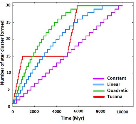
Figure 1: Star formation histories used in this project, based on the star formation histories of classical dSph galaxies, taken from the analysis of the stars in the main sequence described in Weisz et al. (2014)

.

Table 1: Initial conditions and results of our simulations with a cusped DM profile: The first column is the number assigned to the simulation, second column is the dark matter profile, third column is the SFH, fourth column is the star formation efficiency, fifth, sixth and seventh column are the fitted parameters of the Sersic profile, eighth column is the clumpiness value and the last column is the number of surviving star clusters.

Nr.	N/P	SFH	SFE	$\Sigma_{\rm eff}$	$R_{\rm eff}$	n	C	Surv.
				$\left[\frac{{\rm M}_{\odot}}{{\rm pc}^{2}}\right]$	[pc]			SC(s)
1	N	cte	0.2	0.808 $\pm$ 0.033	234 $\pm$ 7	0.696 $\pm$ 0.026	0.046	0
2	N	cte	0.2	0.767 $\pm$ 0.036	234 $\pm$ 8	0.784 $\pm$ 0.030	0.046	0
3	N	cte	0.2	0.574 $\pm$ 0.033	292 $\pm$ 12	0.660 $\pm$ 0.034	0.048	0
4	N	cte	0.2	0.699 $\pm$ 0.039	249 $\pm$ 11	1.020 $\pm$ 0.039	0.035	0
	N	ALL	0.2	0.712 $\pm$ 0.102	252 $\pm$ 27.42	790 $\pm$ 0.161	0.043 $\pm$ 0.005	0
5	N	lin	0.2	0.891 $\pm$ 0.032	227 $\pm$ 6	0.548 $\pm$ 0.022	0.028	0
6	N	lin	0.2	0.796 $\pm$ 0.034	229 $\pm$ 7	0.748 $\pm$ 0.028	0.019	0
7	N	lin	0.2	0.615 $\pm$ 0.017	288 $\pm$ 6	0.554 $\pm$ 0.016	0.036	0
8	N	lin	0.2	0.848 $\pm$ 0.042	226 $\pm$ 8	0.850 $\pm$ 0.033	0.020	0
	N	ALL	0.2	0.787 $\pm$ 0.121	242.5 $\pm$ 30.35	0.675 $\pm$ 0.149	0.025 $\pm$ 0.007	0
9	N	quad	0.2	0.765 $\pm$ 0.027	246 $\pm$ 6	0.645 $\pm$ 0.022	0.019	0
10	N	quad	0.2	0.829 $\pm$ 0.032	226 $\pm$ 6	0.703 $\pm$ 0.025	0.014	0
11	N	quad	0.2	0.640 $\pm$ 0.022	280 $\pm$ 7	0.553 $\pm$ 0.020	0.025	0
12	N	quad	0.2	0.842 $\pm$ 0.041	229 $\pm$ 8	0.790 $\pm$ 0.032	0.016	0
	N	ALL	0.2	0.769 $\pm$ 0.092	245.25 $\pm$ 24.78	0.672 $\pm$ 0.099	0.018 $\pm$ 0.004	0
13	N	tuc	0.2	0.778 $\pm$ 0.029	242 $\pm$ 6	0.646 $\pm$ 0.023	0.019	0
14	N	tuc	0.2	0.869 $\pm$ 0.035	219 $\pm$ 6	0.690 $\pm$ 0.025	0.018	0
15	N	tuc	0.2	0.650 $\pm$ 0.022	275 $\pm$ 7	0.559 $\pm$ 0.020	0.037	0
16	N	tuc	0.2	0.921 $\pm$ 0.038	218 $\pm$ 6	0.725 $\pm$ 0.026	0.015	0
	N	ALL	0.2	0.804 $\pm$ 0.118	238.5 $\pm$ 26.73	0.655 $\pm$ 0.071	0.022 $\pm$ 0.009	0
17	N	cte	0.3	0.904 $\pm$ 0.039	220 $\pm$ 7	0.670 $\pm$ 0.027	0.071	2
18	N	cte	0.3	0.723 $\pm$ 0.056	238 $\pm$ 14	0.93 $\pm$ 0.052	0.055	1
19	N	cte	0.3	0.716 $\pm$ 0.070	257 $\pm$ 18	0.543 $\pm$ 0.058	0.061	1
20	N	cte	0.3	0.845 $\pm$ 0.053	222 $\pm$ 10	0.95 $\pm$ 0.043	0.053	3
	N	ALL	0.3	0.797 $\pm$ 0.092	234.25 $\pm$ 17.17	0.773 $\pm$ 0.199	0.060 $\pm$ 0.008	1.75 $\pm$ 0.957
21	N	lin	0.3	0.828 $\pm$ 0.034	233 $\pm$ 7	0.672 $\pm$ 0.026	0.038	0
22	N	lin	0.3	0.746 $\pm$ 0.007	238 $\pm$ 1	0.83 $\pm$ 0.011	0.019	0
23	N	lin	0.3	0.678 $\pm$ 0.025	269 $\pm$ 7	0.569 $\pm$ 0.022	0.045	0
24	N	lin	0.3	0.512 $\pm$ 0.130	306 $\pm$ 60	1.30 $\pm$ 0.183	0.021	1
	N	ALL	0.3	0.691 $\pm$ 0.134	261.5 $\pm$ 33.66	0.842 $\pm$ 0.323	0.030 $\pm$ 0.012	0.25 $\pm$ 0.5
25	N	quad	0.3	0.712 $\pm$ 0.012	254 $\pm$ 2	0.748 $\pm$ 0.017	0.039	0
26	N	quad	0.3	0.878 $\pm$ 0.039	217 $\pm$ 7	0.729 $\pm$ 0.028	0.016	0
27	N	quad	0.3	0.630 $\pm$ 0.021	279 $\pm$ 7	0.623 $\pm$ 0.020	0.031	0
28	N	quad	0.3	0.898 $\pm$ 0.043	219 $\pm$ 8	0.830 $\pm$ 0.032	0.018	0
	N	ALL	0.3	0.779 $\pm$ 0.129	242.25 $\pm$ 29.81	0.732 $\pm$ 0.085	0.026 $\pm$ 0.010	0
29	N	tuc	0.3	0.730 $\pm$ 0.030	250 $\pm$ 8	0.749 $\pm$ 0.026	0.029	0
30	N	tuc	0.3	0.773 $\pm$ 0.008	235 $\pm$ 1	0.786 $\pm$ 0.012	0.022	0
31	N	tuc	0.3	0.605 $\pm$ 0.022	285 $\pm$ 8	0.678 $\pm$ 0.022	0.032	0
32	N	tuc	0.3	0.932 $\pm$ 0.046	215 $\pm$ 8	0.791 $\pm$ 0.033	0.017	0
	N	ALL	0.3	0.760 $\pm$ 0.135	246.25 $\pm$ 29.54	0.751 $\pm$ 0.052	0.025 $\pm$ 0.006	0

Table 2: Initial conditions and results of our simulations with a cored DM profile: The first column is the number assigned to the simulation, second column is the dark matter profile, third column is the SFH, fourth column is the star formation efficiency, fifth, sixth and seventh column are the fitted parameters of the Sersic profile, eighth column is the clumpiness value and the last column is the number of surviving star clusters.

Nr.	N/P	SFH	SFE	$\Sigma_{\rm eff}$	$R_{\rm eff}$	n	C	Surv.
				$\left[\frac{{\rm M}_{\odot}}{{\rm pc}^{2}}\right]$	[pc]			SC(s)
33	P	cte	0.2	0.205 $\pm$ 0.013	469 $\pm$ 22	0.825 $\pm$ 0.050	0.107	2
34	P	cte	0.2	0.189 $\pm$ 0.011	493 $\pm$ 21	0.933 $\pm$ 0.048	0.126	2
35	P	cte	0.2	0.130 $\pm$ 0.007	593 $\pm$ 26	0.870 $\pm$ 0.044	0.112	0
36	P	cte	0.2	0.159 $\pm$ 0.005	533 $\pm$ 13	0.929 $\pm$ 0.027	0.082	1
	P	ALL	0.2	0.170 $\pm$ 0.033	522 $\pm$ 54.19	0.889 $\pm$ 0.051	0.106 $\pm$ 0.018	1.25 $\pm$ 0.957
37	P	lin	0.2	0.202 $\pm$ 0.005	462 $\pm$ 8	0.903 $\pm$ 0.021	0.058	0
38	P	lin	0.2	0.200 $\pm$ 0.016	471 $\pm$ 27	0.939 $\pm$ 0.065	0.059	1
39	P	lin	0.2	0.127 $\pm$ 0.003	609 $\pm$ 10	0.855 $\pm$ 0.017	0.069	0
40	P	lin	0.2	0.159 $\pm$ 0.003	547 $\pm$ 9	0.824 $\pm$ 0.017	0.078	0
	P	ALL	0.2	0.172 $\pm$ 0.035	522.25 $\pm$ 69.26	0.880 $\pm$ 0.050	0.066 $\pm$ 0.009	0.25 $\pm$ 0.5
41	P	quad	0.2	0.212 $\pm$ 0.005	451 $\pm$ 8	0.883 $\pm$ 0.020	0.038	0
42	P	quad	0.2	0.206 $\pm$ 0.003	468 $\pm$ 5	0.818 $\pm$ 0.012	0.057	1
43	P	quad	0.2	0.130 $\pm$ 0.002	596 $\pm$ 9	0.869 $\pm$ 0.015	0.065	0
44	P	quad	0.2	0.172 $\pm$ 0.003	520 $\pm$ 8	0.786 $\pm$ 0.016	0.054	0
	P	ALL	0.2	0.180 $\pm$ 0.037	508.75 $\pm$ 65.15	0.839 $\pm$ 0.045	0.053 $\pm$ 0.011	0.25 $\pm$ 0.5
45	P	tuc	0.2	0.257 $\pm$ 0.010	408 $\pm$ 11	0.734 $\pm$ 0.030	0.060	1
46	P	tuc	0.2	0.234 $\pm$ 0.014	440 $\pm$ 18	0.736 $\pm$ 0.045	0.071	1
47	P	tuc	0.2	0.149 $\pm$ 0.006	546 $\pm$ 16	0.789 $\pm$ 0.029	0.096	0
48	P	tuc	0.2	0.151 $\pm$ 0.004	552 $\pm$ 10	0.924 $\pm$ 0.019	0.052	0
	P	ALL	0.2	0.197 $\pm$ 0.055	486.5 $\pm$ 73.38	0.795 $\pm$ 0.089	0.069 $\pm$ 0.019	0.5 $\pm$ 0.577
49	P	cte	0.3	0.336 $\pm$ 0.033	350 $\pm$ 26	0.504 $\pm$ 0.057	0.183	12
50	P	cte	0.3	0.241 $\pm$ 0.022	446 $\pm$ 33	0.657 $\pm$ 0.054	0.186	13
51	P	cte	0.3	0.206 $\pm$ 0.029	456 $\pm$ 50	0.562 $\pm$ 0.081	0.330	9
52	P	cte	0.3	0.309 $\pm$ 0.029	359 $\pm$ 25	0.494 $\pm$ 0.053	0.154	6
	P	ALL	0.3	0.273 $\pm$ 0.059	402.75 $\pm$ 55.98	0.554 $\pm$ 0.074	0.213 $\pm$ 0.079	10 $\pm$ 3.162
53	P	lin	0.3	0.299 $\pm$ 0.040	374 $\pm$ 39	0.600 $\pm$ 0.079	0.128	9
54	P	lin	0.3	0.046 $\pm$ 0.026	1427 $\pm$ 72	1.894 $\pm$ 0.378	0.171	11
55	P	lin	0.3	0.149 $\pm$ 0.014	538 $\pm$ 42	0.874 $\pm$ 0.056	0.128	6
56	P	lin	0.3	0.193 $\pm$ 0.021	483 $\pm$ 43	0.807 $\pm$ 0.064	0.120	5
	P	ALL	0.3	0.171 $\pm$ 0.104	705.5 $\pm$ 485.804	1.043 $\pm$ 0.578	0.136 $\pm$ 0.023	7.75 $\pm$ 2.753
57	P	quad	0.3	0.288 $\pm$ 0.017	387 $\pm$ 18	0.641 $\pm$ 0.035	0.132	9
58	P	quad	0.3	0.166 $\pm$ 0.026	539 $\pm$ 73	1.045 $\pm$ 0.099	0.119	10
59	P	quad	0.3	0.160 $\pm$ 0.013	534 $\pm$ 37	0.720 $\pm$ 0.050	0.102	5
60	P	quad	0.3	0.185 $\pm$ 0.016	501 $\pm$ 36	0.780 $\pm$ 0.051	0.089	5
	P	ALL	0.3	0.199 $\pm$ 0.059	490.25 $\pm$ 70.86	0.796 $\pm$ 0.175	0.110 $\pm$ 0.018	7.25 $\pm$ 2.629
61	P	tuc	0.3	0.341 $\pm$ 0.026	346 $\pm$ 19	0.526 $\pm$ 0.043	0.122	9
62	P	tuc	0.3	0.221 $\pm$ 0.039	440 $\pm$ 64	0.847 $\pm$ 0.108	0.136	9
63	P	tuc	0.3	0.183 $\pm$ 0.029	483 $\pm$ 61	0.677 $\pm$ 0.092	0.293	7
64	P	tuc	0.3	0.064 $\pm$ 0.009	927 $\pm$ 114	1.728 $\pm$ 0.096	0.179	5
	P	ALL	0.3	0.202 $\pm$ 0.114	549 $\pm$ 258.41	0.944 $\pm$ 0.538	0.182 $\pm$ 0.077	7.5 $\pm$ 1.914

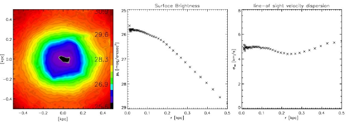
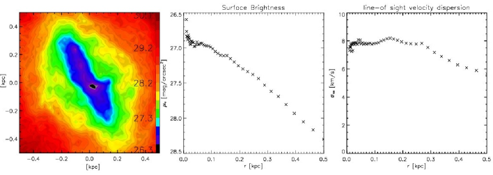
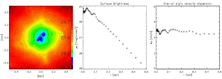
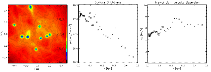
Figure 2: Characteristics of the final object inside a radius of 500 pc, the left panel is the shape of the final object with color bars for the magnitudes of surface brightness, the centre panel shows the radial surface brightness profile and the right panel is the radial velocity dispersion profile, both measured in concentric rings. First row shows a simulation with a a linear SFH, SFE=20% and NFW halo (simulation 5), second row: quadratic SFH, SFE=20% and cored DM halo (simulation 41), third row: constant SFH, SFE=30% and NFW halo (simulation 20), last row: constant SFH, SFE=30% and cored DM halo (simulation 50). The simulation numbers are according to the list in Tab. 1 & 2.

We consider the following setup for our simulations:

1. [i]

2. Simulations with a cusped dark matter halo, as cosmological simulations predict, use a Navarro, Frenk & White (NFW; Navarro et al., 1997) profile, using 1,000,000 particles according to the recipe described in Dehnen & McLaughlin (2005). We use a scalelenght for the halo of $R_{\rm s,h}=1$ kpc and define an enclosed halo mass within 500 pc of $M_{500}=10^{7}$ M_⊙, following the fiducial model described in Assmann et al. (2013a). Using a standard value for $H_{0}=70$km s^-1Mpc^-1 and $r_{\rm vir}=r_{200}$, we obtain a virial radius of $r_{\rm vir}=12.7$ kpc, i.e. the concentration of the halo is $c=12.7$, which agrees with the range of values found with dSph galaxies of 5-20. The total mass of the halo out to the virial radius amounts to $2.3\times 10^{8}$ M_⊙.

3. Simulations with a cored dark matter halo use a Plummer sphere profile (Plummer, 1911), using 1,000,000 particles, with a scale-length (Plummer radius) of $R_{\rm s,h}=1$ kpc, and an enclosed mass within 500 pc of $M_{500}=10^{7}$ M_⊙. For the Plummer profile we use a cut-off radius of $R_{\rm cut}=5$ kpc, which contains more than 94% of the total mass of a Plummer sphere, accounting in our case to a total mass of the halo of $1.1\times 10^{8}$ M_⊙.

4. For the luminous component, the star clusters, we use $N=30$ star clusters. This number is chosen arbitrarily, because the previous results of Assmann et al. (2013a, b), show no significant differences using different numbers of SCs. As it is claimed that dSph galaxies had low star formation rates and therefore also a low SFE (Bressert et al., 2010), we form rather low mass open clusters and associations than massive SCs. Each SC is modelled as a Plummer sphere (Plummer, 1911), with 100,000 particles using the recipe of Aarseth et al. (1974). The SCs have a Plummer radius (half light radius) of $R_{\rm pl}=4$pc and a cut-off radius of 25pc. This is similar to the radii found for young SCs in the Antennae (Withmore et al., 1999).

5. We mimic the gas-expulsion of the SCs by artificially reducing the mass of each particle until the final mass is reached after one crossing time, i.e. 4 Myr. As the mass in lost gas is negligible compared to the DM mass we do not take this mass further into account. The final mass in stars (of all SCs) after this mass loss amounts to $4.5\times 10^{5}$M_⊙, which is a typical stellar mass of one of the classical dSph (e.g. Mateo M. (1998)). We perform simulations with SFEs of 20% and 30%. Therefore, the initial mass of each SC in its embedded phase is $5\times 10^{4}$ M_⊙ for SFE = 30% and $7.5\times 10^{4}$M_⊙ for SFE = 20%. Note, that this results in a particle resolution in our simulation which is slightly better than reality, i.e. more star particles than actual stars (see explanation below).

6. The star clusters themselves are distributed in virial equilibrium inside the halo according to a Plummer distribution. This is made for simplicity, because we do not know exactly in which virial state the SCs form with respect to the halo and we expect more star clusters to form in the centre than in the outer parts. The distribution has a scale-length of $R_{\rm pl,sc}=0.25$ kpc and a cut-off radius of $R_{\rm cut-off}=1.125$ kpc. The initial orbital velocities are obtained from the Jeans equation:

   $$\sigma_{r,i}^{2}(r) = \frac{1}{\rho_{i}(r)}\int_{r}^{rc}\frac{GM_{tot}(r^{\prime})}{r^{2}}\rho_{i}(r^{\prime})dr^{\prime},$$ (1)

   where $M_{\rm tot}$ correspond to the total mass given by the sum of the mass of all SCs and the mass of the DM halo. We do not assume any anisotropy in spatial nor in the velocity distribution. Also we do not take into account that the SCs might form in a disc-like structure showing angular momentum in their distribution, as we assume that the gas distribution on the small scales of a dSph is rather supported by pressure than rotation. With this assumption we differ from most of the previous models in which dSph galaxies are simply the evolutionary outcome of harassed dwarf disc galaxies, which lost their angular momentum because of gravitational forces.

7. To mimic the star formation histories we insert the star clusters at different times into the simulations. We probe four different star formation histories. Fig. 1 shows the SFHs used in this project. The first is a constant SFH in which we insert the star clusters one by one over the whole 10 Gyr of evolution in equally spaced time intervalls. The second SFH mimics a linearly declining SFR and the third a quadratic decline in SFR. I.e. in both cases the majority of SCs are inserted at early times of the simulation and only a few get inserted at late times. The last SFH mimics a double burst as implied for Tucana. Half of the SCs get inserted at the beginning of the simulation and the second half after 5 Gyr, i.e. half of the simulation time. For the common SFH of dSph galaxies, the single burst at very early times, we refer to the models of Assmann et al. (2013a, b) in which the simulations start with all SCs from the beginning.

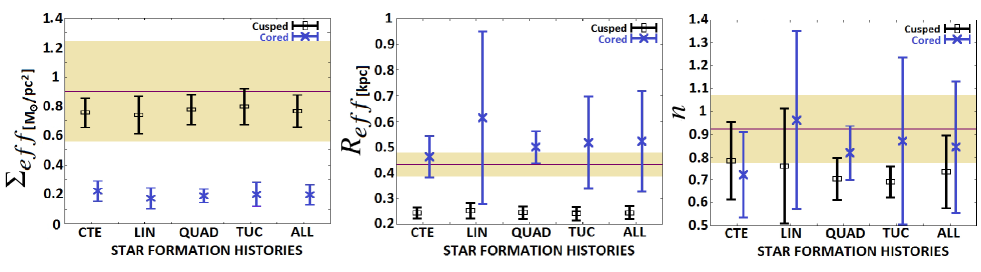
Figure 3: Mean values of the Sersic profile fits for different DM halos and SFHs. The data points are mean values from all simulations using the same DM halo and both values of SFE (0.2 and 0.3). Previous and our results have shown that the profile parameters do not depend on the SFE used. As can be seen in the panels, it also does not depend on the SFH used. Therefore, we plot as the last point the mean value for all simulations with the same DM halo, independent of SFE and SFH. Black bars are for cusped DM halos and blue crosses are for cored DM halos, the purple line shows the results of the previous work (Assmann et al., 2013b). The left panel shows the effective surface brightness, the middle panel the effective radius and the right panel the Sersic index $n$.

We simulate the cluster complex within the DM halo using the particle mesh code Superbox (Fellhauer et al., 2000). Superbox has two levels of high resolution sub-grids. The highest resolution grid has a chosen resolution (i.e. cell-length) of 8.3 pc for the dark matter halo and 0.41 pc for the star clusters and covers the central area of the halo or the SCs completely, respectively. The medium resolution grid has a cell-length of 41 pc for the DM halo and 4.1 pc for the SCs. Finally, the outermost grid covers the complete area beyond the virial radius of the dark matter halo with a resolution of 830 pc. The time-step is fixed at 0.25 Myr to resolve the internal dynamics of the SCs and we simulate for 10 Gyr.

As the SCs dissolve immediately, two-body relaxation effects are not important, i.e. we are able to use a fast particle-mesh code. A particle mesh-code naturally neglects close encounters between particles (which here are rather representations of the phase space than actual single stars) and is therefore called collision-less. That the particles are phase-space representations makes it (in our case) possible to actually use more particles than actual stars. With the same reasoning we can model the DM halo without using an actual number of DM particles.

We run 64 simulations for 10 Gyr. For the setup of the simulations we refer to the first columns in Tabs. 1 & 2.

3 Results

In Fig. 2, we show a set of four different simulations as examples. The examples show a wide range of different outcomes from our simulations, but all except the last one show properties similar to the classical dSph galaxies of the MW.

Our models predict objects with different shapes and in Fig. 2 we show: a) a final object nearly spherical in which all the SCs have dissolved (simulation number 5), b) a very elongated final object in which all SCs have dissolved, but some of them had similar orbital planes causing a flattened profile (number 41), c) a double cored final object with two high density peaks in the centre (number 20) and finally d) a final object which can not resemble the properties of classical dSph because the SCs did not dissolve completely (number 50). The number point to the respective simulations in Tabs. 1 & 2.

In the next subsections we will focus on the analysis of the surface brightness profile, the velocity dispersion, the shape of the final object and the surviving SCs. A summary of important results can be found in Tabs. 1 & 2.

3.1 Surface brightness profile

We fit the surface brightness profile of our simulations using a Sersic profile:

$$\Sigma(R) = \Sigma_{\rm eff}\exp\left(-b_{\rm n}\left[\left(\frac{R}{R_{\rm eff}}\right)^{\frac{1}{n}}-1\right]\right)$$ (2)

$$b_{\rm n} = 1.9992n-0.3271$$

with $R_{\rm eff}$ the effective radius and $\Sigma_{\rm eff}$ the surface density at the effective radius. This profile has the advantage of having three free parameters, so our simulations can be fitted easily. The index $n$ gives us information about the shape of the dSph galaxy. In the case $n\approx 1$, we will have an exponential profile for the surface density distribution, as it is observed in classical dSph galaxies (Caon et al., 1993; Jerjen et al., 2000; Walcher et al., 2003).

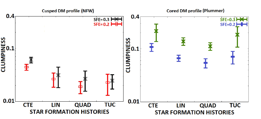
Figure 4: Mean clumpiness values for different SFHs and SFEs in a cusped DM halo (left panel) and a cored DM halo (right panel). Simulations with SFE=30% are shown in black and green crosses and SFE=20% are denoted by red and blue bars. Note, that the $y$-axis has a logarithmic scale. Cored DM halo models have higher clumpiness values than cusped models, furthermore recent star formation and higher SFE give us more inhomogeneous final objects.

Surface brightness profiles show integrated light along a line-of-sight. As we do not know the actual line of sight, towards our theoretical objects, we project our objects along the three different Cartesian coordinates. Then we bin the data in 50 concentric rings with logarithmically equally spaced widths from the centre out to $0.5$ kpc. We calculate a mean value profile with one sigma deviations from the three projections. That way we avoid to take the elliptic shape of the contours into account and we do not need to project along the major axes of the object. This is the same procedure to produce the data as described in Assmann et al. (2013a, b), i.e. it is possible to compare our data directly with the previous results. Furthermore, as stated above, we do not know the exact orientations the classical MW dSph are presenting towards us. As long as those orientations are unclear, it makes more sense to compare our mean model profiles to the randomly oriented real dSph galaxies, than to compute values along the main axes of our objects.

In Fig. 3, we show the correlation between the three parameters of the Sersic profile ($\Sigma_{\rm eff}$, $n$ and $R_{\rm eff}$), fitted to our models, versus their SFH for the different DM halos. Our results do not show any dependence of the SFE used, thereby confirming the results of Assmann et al. (2013a, b), and the mean values shown are already averages over the different SFEs used. We also see that there is no dependency on the SFH in our data. Therefore, the final data point in each panel shows a mean value of all simulations using the same DM halo. The purple lines are the mean values of the previous study by Assmann et al. (2013a, b). The one sigma deviations are shown as shaded areas around the mean. There is indeed one word of caution left. In the presentation of their fiducial model in Assmann et al. (2013a), the mean values quoted there are similar to the cored profile results in our study. Only if we use all simulations with the same parameters ($M_{500}$, $R_{\rm h}$ and $R_{\rm sc}$) from Assmann et al. (2013b) we obtain similar results as in our study. This shows that the random placement of a small $N$ number of SCs can lead to a huge variation in the final results, even when using the same over-all parameters. As an example we quote the minimum and maximum values for this parameter set from Assmann et al. (2013b, see results given in the tables): for $\Sigma_{\rm eff}$ we obtain values from $0.1$ to $3$ M_⊙ pc^-2, for $n$ from $0.4$ to $2.1$ and for $R_{\rm eff}$ from $140$ to $740$ pc.

Taking this words of caution into account, we still see that the mean effective surface brightness is higher for NFW halos than for the cored Plummer halos. The opposite is true for the effective radius; cored profiles show about twice the effective radius than cusped profiles. Here we are in disagreement with Assmann et al. (2013b), which see no significant differences between the two types of profiles. The answer to this riddle is that for our study we have more simulations per parameter set (but a smaller range of parameters) than used in Assmann et al. (2013b).

Fig. 3 shows clearly that cusped DM halos give us higher values for $\Sigma_{\rm eff}$, and lower for $R_{\rm eff}$ than cored DM models. This is because a cusped profile has a high density in the centre and the stars are more likely to get stripped in the central part of the DM halo than in a cored DM profile.

We see that the Sersic index $n$ has no dependency on any initial parameter. It shows always mean values around 1, independently of the SFH or DM halo. This means that our resulting objects have approximately an exponential surface brightness distribution, like the dSph galaxies of the Local Group (Walcher et al., 2003; Jerjen et al., 2000; Caon et al., 1993).

Taking all simulations into account we obtain the following mean values: For our NFW halo models a Sersic index of $n=0.74\pm 0.16$, an effective radius of $R_{\rm eff}=0.245\pm 0.026$ kpc and a surface density at this radius of $\Sigma_{\rm eff}=0.77\pm 0.11$ M_⊙ pc^-2. For the cored Plummer profiles as DM halo we measure $n=0.84\pm 0.29$, $R_{\rm eff}=0.52\pm 0.20$ kpc and $\Sigma_{\rm eff}=0.196\pm 0.068$ M_⊙ pc^-2.

Photometrical observations of the dSph galaxies in the Local Group show that we can find different sizes of these galaxies. For example, the effective radii of Draco, UMi, Sculptor and Fornax are 180, 200, 110 and 460 pc, respectively (Mateo M., 1998; Irwin & Hatzidimitriou, 1995), i.e. span the complete range between our cusped and cored models.

Furthermore, in this study we kept the radius of the SC distribution constant in all simulations. As stated in Assmann et al. (2013b) our models predict an effective radius of the luminous component of about/up to twice the size of the star cluster distribution. Our new results show that this is still true for cored DM halo profiles but are closer to equal in size in the case of NFW halos.

3.2 Clumpiness

We now consider the clumpiness parameter to characterise the shape of our resulting object. The clumpiness is a way to measure the inhomogeneity in the distribution of stars. We use the method explained in Conselice (2003) and construct a smooth elliptic model which fits our simulation result, using the IRAF routine ELLIPSE. Then, we subtract this smooth model from our data and sum the positive residuals. The ratio between these residuals and the original data is the clumpiness C:

$$C = \frac{\Sigma_{\rm allpix}m_{\rm residual,pixel}}{\Sigma_{\rm allpix}m_{\rm original,pixel}}.$$ (3)

In Fig. 4, we show the relationship between the clumpiness of our models the SFH, SFE and DM distribution. The left panel is for cusped DM halo models and the right panel is for cored DM haloes. Crosses are for SFE=30% and bars for SFE=20% and in the x-axis we plot the SFH.

First, we observe that all our simulations lead to low values of the clumpiness parameter. This is a hint that the substructure we see in the brightness maps of our model might be only visible due to our larger than reality particle resolution. But those faint structures in our simulations are definitely real and not due to noise and the brighter ones should be observable.

These plots show that models with recent star formations have higher values of clumpiness than models without. The later the star clusters form the less time they have to dissolve and form a homogeneous final object. Furthermore, the value of clumpiness depends on the SFE: If the SFE is higher (30%) the star clusters will need more time to dissolve after gas-expulsion leading to higher values of clumpiness than models with low SFE (20%).

We observe that in a cored DM profile we measure higher clumpiness parameters than in cusped models. This is a consequence that Plummer models have central crossing times larger than models with NFW profile and less interaction time to erase substructure. Also a cusp is more efficient in dispersing stars from their original orbits, leading to a more homogeneous distribution with time.

The large error bars in the clumpiness value for cored DM halos and SFE=30% are due to the high number of surviving SCs, so our final object is not easy to fit.

It is hard to compare our results with the classical dSph of the MW as there is no determination of their clumpiness published, but we observe in classical dSph the same elongations, twists, deviations from ellipses and/or double cores (see e.g. Irwin & Hatzidimitriou, 1995) that elevate the clumpiness values in our models.

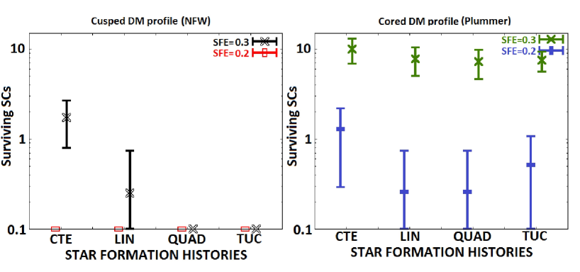
Figure 5: Number of surviving SCs vs. SFH; the left panel shows simulations with a cusped DM halo profile and in the right panel are the simulations with a cored DM profile. Red and blue bars denote SFE=20% and black and green crosses SFE=30%. The $y$-axis has a logarithmic scale and therefore 0 surviving SCs are marked as 0.1 in the plots. In cusped DM halos the SCs dissolve easily and we do not see any survivors in simulations with no recent star formation. In cored DM halos we have several surviving star clusters even with a SFE=20% and no recent star formation.

3.3 SC dissolution

Some of our final objects have several surviving SCs which are orbiting the centre of the DM halo. Those SCs can survive either because they need more time to get dissolved or because their orbit is very close to the centre of the DM halo where the stars struggle to escape the deep potential well of the halo. Also cored DM halos need more time to dissolve SCs than cusped DM halos as shown also in e.g. (Peñarrubia et al.2009) and Amorisco (2017). We consider a SC to be dissolved if it has less than 10% of particles bound. In Fig. 5 we show the correlation between the number of surviving SCs, the SFH, SFE and the DM profile.

In simulations with low SFE (20%) we see no surviving SCs in cusped DM halos, because it only takes them a few hundred Myr to dissolve. In simulations with cored DM haloes, the dissolution time of SCs is significantly longer. Therefore, especially in simulations with late star formation (constant SFH) most of the SCs, inserted last, have no time to dissolve.

In simulations with high SFE (30%), the number of surviving SCs is higher. For cusped DM profiles we need approximately $1$ Gyr to dissolve the SCs. For cored DM profiles the number of surviving SCs is much higher, and there are some star clusters which cannot be dissolved even after $10$ Gyr if the apocentric distance is small ($<300$ pc). In Fig. 6 we show the process of dissolution of a SC orbiting the centre of a DM halo. We see that the SC is expanding while it is orbiting the centre of the DM halo. It expands when near the centre and contracts again while far from the centre. In that sense we do see sometimes fluffy density enhancements, which could be mistaken for an extended cluster. In reality we see a dissolved SC close to its apocentre, where the original stars of the SC are in compressed tidal tails, mimicking a density enhancement at its current position. This effect is more pronounced, if clusters are orbiting closer to the centre of the DM halo.

Intuitively, we have more surviving SC in simulations with recent star formation because the last SCs which are placed within the DM halo have less time to get dissolved completely in comparison to the older SCs.

The time to erase a SC will vary depending on its orbit, SFE and the DM profile, in Fig. 7 we plot the correlation between the dissolving time and the apocentric distance for both DM halos and SFEs. Filled bars and crosses are for the cored DM haloes (SFE=20% and 30% respectively), while open bars and crosses denote cusped haloes. In order to say that a SC is dissolved we measure the time when less than 10% of the particles are bound.

Fig. 7 shows that for a cusped DM profile the dissolving time is always lower than in the corresponding cored simulations and will not take more than 1 Gyr, even if the SFE is high (30%). Furthermore, we see that in cusped simulations the dissolution time is almost independent from the apo-centric distance of the SCs. On the other hand for cored DM profiles the dissolution time is higher if the apo-centric distance of the orbit is small ($<300$ pc), this is because the stars of the SC can not escape easily from the potential well of the core, while at the same time there is no steep potential difference within the core. So the stars get less dispersed and get compressed along the orbit and re-captured close to the apo-centre. SCs with large apo-centric distances (outside the central area) in cored simulations will indeed suffer from strong potential gradients along their orbit and therefore are dissolving faster. If we increase the SFE to 30%, the SCs with the smallest orbits will need more than 10 Gyr to get dissolved.

The presence of surviving SCs in our simulations, could give us predictions for future observations to corroborate our formation scenario, for example in Fornax there are five old SCs discovered orbiting this galaxy and in several dwarf galaxies we see young star clusters (e.g. Grasha et al., 2017).

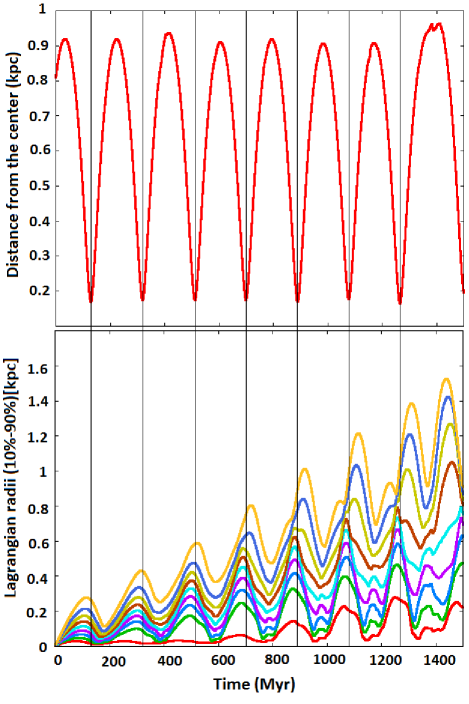
Figure 6: This plots are taken from a SC in a cored DM halo and a SFE=30%. The top panel shows orbit of the SC, i.e. the distance to the centre of the DM halo, and the bottom panel the Lagrangian radii (10%-90%), measured for the original SC particles with respect to the present SC location. We see that the SC is expanding and contracting while it is orbiting the DM halo. The SC expands while it is passing through peri-centre and contracts at its apo-centre.

3.4 Velocity space

The dSph satellite galaxies of the MW are close enough to obtain high resolution measurements of their line-of-sight velocity dispersions, which are in the order of 5 to 10 km s^-1 (Walker et al., 2007). We compare the line of sight velocity dispersion profile of the final objects with the typical velocity dispersion observed in classical dSph galaxies.

To measure the line-of-sight velocity dispersion of our models we consider the mean values of the velocity dispersion of all pixels within a radius of 10 pc and 500 pc from the centre of the object. This mean value is calculated by considering the mean velocity dispersion along all three coordinate axis because the orientation of our objects is unknown. With this method we also keep the same analysis of the data as in our previous studies to be able to compare our results.

In the right panels of Fig. 2, we show the line-of-sight velocity dispersion profiles for some of our simulations. These profiles have been obtained considering the mean value of the line of sight velocity dispersion of pixels within concentric rings with varying radius. In all simulations the velocity dispersion profiles are always more or less flat, except in models with a high quantity of surviving SCs like Fig. 2 (lowest panels), all of our models show velocity dispersion in the range of 5 to 12 km s^-1, which is in agreement with observations.

Looking at the outer part of the profiles we observe different types of behaviour in the velocity dispersion. We get outer profiles (beyond 1 kpc) where the velocity dispersion falls slowly in some cases, while in others the dispersion stays flat. We see a similar behaviour in the MW’s dwarf galaxies. In Sextans we see a slight drop in velocity dispersion around 1 kpc, while Sculptor, Draco and Fornax show flat profiles (Walker et al., 2007, their figure 2).

In the inner part, some of our simulations show wiggles and bumps in the dispersion profile. While the observers always try to fit smooth curves, thus implicitly assuming that any bumps seen in the profiles are merely due to statistical noise (e.g. Sculptor, Draco or Carina), in our models, the strange bumps in the observed profiles are not due to noise in the observed data sets. According to our formation theory they are a natural product of the formation scenario proposed. For a detailed investigation of this phenomena we refer to our previous publications (Assmann et al., 2013a, b).

Finally, in the central part we see the same behaviour as shown in the multitude of MW’s dwarf galaxies. Some of our models have a central dip in the velocity dispersion profile like in Sextans or Draco. Others show a rising central velocity dispersion. We do not see a similar behaviour with the classical dwarf spheroidal of the MW but there are hints that some of the faint dwarfs galaxies have an elevated central velocity dispersion.

These results show clearly that our models are well suited to reproduce the formation of dSph galaxies. We can show that we can reproduce the dynamics of the different dwarf galaxies with our models.

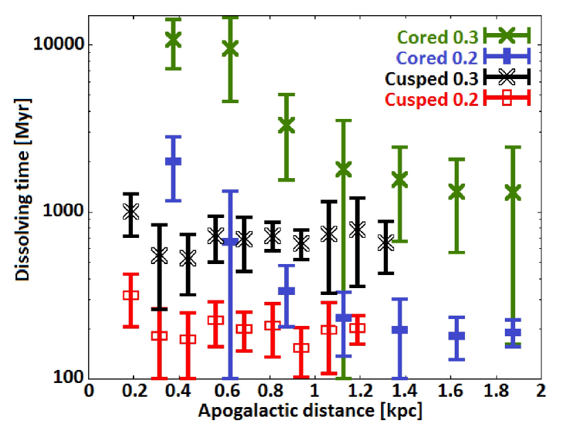
Figure 7: Dissolution time vs. apo-centric distance: This plot shows the dissolution time of the star clusters according to their orbit, dark matter profile of the halo and SFE. Filled bars and crosses are for cored DM halos and a SFE of 0.2 or 0.3 respectively, open bars and crosses are for cusped DM halos with a SFE of 0.2 and 0.3 respectively. We see that the dissolution time is always longer for cored than for cusped halos and longer for higher SFEs. Furthermore, we see a clear trend in the cored simulations that SCs orbiting closer to the centre (small apo-centres) have significantly larger dissolution times.

4 Discussion

Our simulations can resemble the observed properties of classical dSph, as for example an exponential surface brightness profile and a flat velocity dispersion in the range of 5 to 12 km s^-1. Furthermore, we can resemble specific properties seen in some dSph, as for example off-centre nuclei (Sextans), secondary density peaks (Ursa Minor) or dents in the contours (Draco).

An important feature of our simulations is the presence or absence of surviving SCs. We identify three parameters which can be responsible for the survival of a star cluster. The most obvious one is a high SFE, which automatically leads to survival of the gas-expulsion phase. In our simulations, the SFEs used are below the threshold, which is usually believed to produce a surviving star cluster, even though 30% is close to the theoretical limit. Our simulations definitely show that lower SFEs lead to less or none surviving SCs. The next best reason should be that in the case of more recent SFH some SCs have not enough time to get completely dissolved. Again, we see this trend in our simulations. But, we identify a third possibility for SCs to survive and that is in the very centre of a cored DM halo. A central core does not disperse the stars of the SC from their original orbit and so we see SC remnants, especially if the SC is close to its apo-centric distance. This might be a hint how to support the formation of nuclei in dwarf galaxies.

Our simulations provide a possible solution to why some dSph galaxies have orbiting star clusters and why some of them do not, and this could be a hint to looking for faint surviving SCs in other dSph with future telescopes. As the majority of dSph galaxies do not show associated SC, with the exception of Fornax and Sagittarius, we can deduce, that the SCs inside the DM halos have formed with low SFEs ($<30$%) and most likely in a cusped DM profile as predicted by $\Lambda$-CDM.

The absence of surviving SCs in the observed dSph and the high presence of them in our cored simulations could be a hint for the solution of the cusp-core problem, which is a mismatch in the DM halo profiles between the prediction of cosmological $\Lambda$-CDM simulations, which say that the DM halos have to follow a cusped profile, and the observed kinematic data in dSphs which hints to the notion that the DM profile is possibly cored. In our models the SCs were dissolved more quickly in a cusped profile than in a cored DM halo, this could be a hint of the existence of a mechanism (e.g. feedback, modifications of the nature of dark matter) that eliminates the cusp in DM halos, as some authors claim (e.g. Governato et al., 2010). As we are not performing any sophisticated combined DM and hydrodynamical simulations such transformations from cusped to cored halos and why they are happening are beyond the scope of this study.

Finally, we have to keep in mind that our models make a lot of simplifications, for example, we put the distribution of SCs into virial equilibrium within the DM halo for simplicity, because we do not know in which virial state the SCs are formed and also they follow a Plummer distribution because we expect to form more SCs in the centre of the DM halo than further out. Also we assume that all SCs have a Plummer sphere distribution, which is a good approximation to model a SC. Also all SCs have the same mass. In reality, we would expect that in dSphs with low a star formation rate (SFR) we produce more and smaller SCs and with high SFR we would produce less and more massive SCs. Furthermore, objects with recent star formation are also the ones showing low SFRs and therefore the SCs would be easier to destroy. So we overestimate the number of surviving SCs in these simulations.

We assume the same SFE for each SC, and after the gas-expulsion the gas is lost to nowhere. This is justified because the mass of the gas is negligible with respect to the mass of the DM halo.

Another simplification of our models is that we use SUPERBOX, a particle mesh code which do not take in account two body interactions. It is useful in our case because a dSph galaxy is a collision-less system and the SCs are a collisional system only in their first 4 Myr before gas-expulsion, so we can neglect these interactions.

Our previous models (Assmann et al., 2013a, b) were subject to questions, as we do not include any mass-metallicity relation found in the dwarf galaxy population. Metallicity information is virtually impossible to include in a pure stellar dynamical simulation, but with our new models we show that our previous results are not altered by including different observed SFHs. Still our models are purely stellar dynamical, but now one could include analytically ones favourite astro-chemical model to derive the yields for the later generations of SCs and paint the phase-space elements of our simulations according to their metal content.

In this paper we do not discuss the ellipticities, asymmetries, A4 parameters or what we have dubbed fossil remnants in the velocity space of our models. These parameters were discussed in detail in Assmann et al. (2013b) and the simple addition of a SFH to our models does not change the findings of our previous manuscript.

5 Conclusions

In this paper we test the possible scenario for the formation of dSph galaxies proposed by Assmann et al. (2013a, b) by adding different SFHs to the numerical simulations. In our simulations we consider the evolution of 30 star clusters placed at different moments in time into our simulations to mimic the SFHs. The SCs are dissolving within a cored or a cusped dark matter halo. Also we study the effect of different SFEs (20% and 30%) for those SCs.

We observe that after 10 Gyr of evolution we get an object that resembles the properties of a classical dSph galaxy if we have enough time to dissolve the SCs.

In our models with a low SFE=20% and a DM halo with a NFW profile, the SCs are dissolved in less than 300 Myr, so we can resemble the properties of a classical dSph even if we have recent star formation histories. Models with a cored DM halo following a Plummer sphere profile, need more time to dissolve the SCs ($\approx 500$ Myr), and if the apo-centric distance of these SCs is near to the centre of the DM halo ($<300$ pc), they will need approximately 2 Gyr to get dissolved. So we can resemble the properties of a classical dSph only if we have no recent star formation.

In our models using SCs with a high SFE=30% and a DM halo following a NFW profile, the SCs need approximately between 300 Myr to 1 Gyr to dissolve, and again as we do not see surviving SCs in classical dSph. On the other hand, models with a cored DM profile and SCs with a SFE=30%, can not resemble the properties of classical dSph, because some of the SCs cannot dissolve if their apo-centric distance is close to the centre of the DM halo, they need more than 10 Gyr to dissolve completely, but this could be a hint to explain the formation of massive dSph galaxies like Fornax, with 5 orbiting SCs, or Sagittarius.

In all our models even if we have surviving SCs, we obtain surface brightness profiles as observed in classical dSph. We use a Sersic profile to fit the surface brightness profile of our final objects and get effective radii similar to the observed ones in dSph with a mean value of $245\pm 26$ pc for cusped and $523\pm 195$ pc for cored profiles, also we get values of the $n$ index close to unity ($n=0.74\pm 0.16$ for cusped and $n=0.84\pm 0.29$ for cored), this means that our final objects have exponential surface brightness profiles, as observed in dSphs.

Furthermore, all our simulations show a velocity dispersion in the observed range of classical dSph, between 5-12 km s^-1, and dispersion profiles which remain flat independent of the radius. Another important feature is that we see wiggles and bumps in the data. In observational papers these wiggles and bumps are smoothed over but according to our scenario some of them could be real. In reality we see similar bumps in Carina, Leo I and Sculptor (Walker et al., 2009).

Our models give a hint to the cusp-core problem, as the SCs are more likely to get dissolved in a cusped DM halo, and observations hint that DM halos of dSph could follow a cored profile. We suspect that there could be a mechanism that eliminates the cusp after dissolving all the SCs and form a cored DM profile.

Our simulations show that our formation scenario works even if using different SFHs, DM halo profiles and different SFE to dissolve the SCs and we are not only able to reproduce the observational data that we have today, but provide observers with predictions for future observations.

Acknowledgements: AA thanks R. Dominguez, B. Reinoso and N. Araneda for their help with SUPERBOX. AA thanks his friend N.P. Less for the interesting discussion during the realisation of this work. AA and FU acknowledge financial support from Conicyt through the project PII20150171. MF acknowledges financial support through Fondecyt grant No. 1130521, Conicyt PII20150171 and BASAL PFB-06/2007.

References

- Aarseth et al. ( 1974) Aarseth S.J., Henon M., Wielen R., 1974, A&A, 37, 183
- Amorisco (2017) Amorisco N.C., 2017, ApJ, 844, 64
- Assmann et al. (2013a) Assmann P., Fellhauer M., Wilkinson M.I., Smith R., 2013a, MNRAS, 435.2391
- Assmann et al. (2013b) Assmann P., Fellhauer M., Wilkinson M.I., Smith R., 2013b, MNRAS, 432,274
- Belokurov et al. (2007) Belokurov V. et al., 2007, ApJ, 654, 897
- Boily & Kroupa (2003a) Boily C.M., Kroupa P., 2003a, MNRAS, 338, 665
- Boily & Kroupa (2003b) Boily C.M., Kroupa P., 2003b, MNRAS, 338, 673
- Bonnell et al. (2011) Bonnell I.A., Smith R.J., Clark P.C., Bate M.R., 2011, MNRAS, 410, 2339
- Bressert et al. (2010) Bressert E. et al., 2010, MNRAS, 409, L54
- Caon et al. ( 1993) Caon N., Capaccioli M., D’Onofrio M., 1993, MNRAS, 265, 10132
- Cole et al. (1994) Cole S., Aragon-Salamanca A., Frenk C.S., Navarro J.F., Zepf S.E., 1994, MNRAS, 271, 781
- Conselice (2003) Conselice C. J., 2003, ApJS, 147, 1
- Dehnen & McLaughlin (2005) Dehnen W., McLaughlin D.E., 2005, MNRAS, 363, 1057
- D’Onghia et al. (2009) D Onghia E., Besla G., Cox T., Hernquist L., 2009, Nature, 460, 605
- Fellhauer et al. (2000) Fellhauer M., Kroupa P., Baumgardt H., Bien R., Boily C.M., Spurzem R., Wassmer N., 2000, New Astron., 5, 305
- Gnedin et al. (1999) Gnedin O.Y., Hernquist L., Ostriker J. P., 1999, ApJ, 514, 109
- Goodwin (1997a) Goodwin S.P., 1997a, MNRAS, 284, 785
- Goodwin (1997b) Goodwin S.P., 1997b, MNRAS, 286, 669
- Governato et al. (2010) Governato F., Brook C., Mayer L., Brooks A., Rhee G., Jonsson P., Willman B., Stinson G., Quinn T., Madau P., 2010, Nature, 463, 203
- Irwin & Hatzidimitriou (1995) Irwin M., Hatzidimitriou D., 1995, MNRAS, 277, 1354
- Jerjen et al. ( 2000) Jerjen H., Binggeli B., Freeman K.C., 2000, AJ, 119, 593
- (22) Kauffmann G., White S., Guiderdoni B., 1993, MNRAS, 264,201
- Kleyna et al. (2002) Kleyna J.T., Wilkinson M.I., Evans N.W., Gilmore G., Frayn C., 2002, MNRAS, 330, 792
- Kleyna et al. (2003) Kleyna J.T., Wilkinson M.I., Gilmore G., Evans N. W., 2003, ApJ, 588, L21
- Kleyna et al. (2004) Kleyna J.T., Wilkinson M.I., Evans N.W., Gilmore G., 2004, MNRAS, 354, L66
- Koch et al. (2009) Koch A. et al., 2009, ApJ, 690, 453
- Lada & Lada (2003) Lada C.J., Lada E.A., 2003, ARA&A, 41, 57
- Lada et al. ( 2010) Lada C.J., Lombardi M., Alves J.F., 2010, ApJ, 724, 687
- Lokas (2009) Lokas E.L., 2009, MNRAS, 394, L102
- Mayer et al. (2007) Mayer L., Kazantzidis S., Mastropiero C., Wadsley J., 2007, Nat, 445, 738
- Mateo M. (1998) Mateo M.L., 1998, ARA&A, 36, 435
- McConnachie (2012) McConnachie, A.W., 2012, AJ, 1444
- Munoz et al. (2005) Munoz R.R. et al., 2005, ApJ, 631, L137
- Munoz et al. (2006) Munoz R.R. et al., 2006, ApJ, 649, 201
- Navarro et al. ( 1997) Navarro J.F., Frank C.S., White S.D.M., 1997, ApJ, 490, 493
- Parmentier et al. (2008) Parmentier G., Goodwin S.P., Kroupa P., Baumgardt H., 2008, ApJ, 678, 347
- (37) Peñarrubia J., Walker M.G., Gilmore G., 2009, MNRAS, 399, 1275
- Plummer (1911) Plummer H.C., 1911, MNRAS, 71, 460
- Simon & Geha (2007) Simon J.D., Geha M., 2007, ApJ, 670, 313
- Grasha et al. (2017) Grasha K. et al., 2017, ApJ, 840, 113
- Smith et al. (2011a) Smith R., Slater R., Fellhauer M., Goodwin S.P., Assmann P., 2011a, MNRAS, 416, 383
- Smith et al. (2011b) Smith R., Fellhauer M., Goodwin S.P., Assmann P., 2011b, MNRAS, 414, 3036
- Walcher et al. (2003) Walcher C.J., Fried J.W., Burkert A., Klessen R.S., 2003, A&A, 406, 847
- Walker et al. (2007) Walker M.G., Mateo M., Olszewski E.W., Gnedin O.Y., Wang X., Bodhisattva S., Woodroofe M., 2007, ApJ, 667, L53
- Walker et al. (2009) Walker M.G., Mateo M., Olszewski E.W., Penarrubia J., Evans N.W., Gilmore G., 2009, ApJ, 704, 1274
- Weisz et al. (2014) Weisz D.R., Dolphin A.E., Skillman E.D., Holtzman J., Gilbert K.M., Dalcanton J.J., Williams B.F., 2014, ApJ, 789, 147
- Withmore et al. (1999) Whitmore B.C., Zhang Q., Leitherer C., Fall S.M., Schweizer F., Miller B.W., 1999, AJ, 118, 1551