Two low-order nonconforming finite element methods for the Stokes flow in 3D

Abstract.

In this paper, we propose two low order nonconforming finite element methods (FEMs) for the three-dimensional Stokes flow that generalize the non-conforming FEM of Kouhia and Stenberg (1995, Comput. Methods Appl. Mech. Engrg.). The finite element spaces proposed in this paper consist of two globally continuous components (one piecewise affine and one enriched component) and one component that is continuous at the midpoints of interior faces. We prove that the discrete Korn inequality and a discrete inf-sup condition hold uniformly in the meshsize and also for a non-empty Neumann boundary. Based on these two results, we show the well-posedness of the discrete problem. Two counterexamples prove that there is no direct generalization of the Kouhia-Stenberg FEM to three space dimensions: The finite element space with one non-conforming and two conforming piecewise affine components does not satisfy a discrete inf-sup condition with piecewise constant pressure approximations, while finite element functions with two non-conforming and one conforming component do not satisfy a discrete Korn inequality.

1. Introduction

Given a polygonal, bounded Lipschitz domain $\Omega\subseteq\mathbb{R}^{3}$ with closed Dirichlet boundary $\Gamma_{D}$ and Neumann boundary $\Gamma_{N}=\partial\Omega\setminus\Gamma_{D}$ both with positive two-dimensional measure and some right-hand side $g\in[L^{2}(\Omega)]^{3}$, the three dimensional Stokes problem seeks the velocity $u\in[H^{1}(\Omega)]^{3}$ and the pressure $p\in L^{2}(\Omega)$ with

(1.1) $$\left.\begin{aligned} -2\mu\operatorname{div}\varepsilon(u)+\nabla p&=g\\ \operatorname{div}u&=0\end{aligned}\right\}\;\text{in }\Omega,\quad u|_{\Gamma_{D}}=0,\quad(2\mu\varepsilon(u)-pI_{3\times 3})|_{\Gamma_{N}}\nu=0.$$

Here and throughout this paper, $\mu$ is the viscosity. The symmetric gradient of a vector field reads $\varepsilon(v):=1/2(\nabla v+\nabla v^{T})$ for any $v\in[H^{1}(\Omega)]^{3}$, while $\nu$ denotes the outer unit normal.

Finite element methods (FEMs) for the two dimensional Stokes problem have been extensively studied in the literature, most of stable schemes are summarised in the book [BBF13]. However only little attention has been paid to the three dimensional problem. Here, we only mention the works [Ste87, Bof97, Zha05, GN14, NS16] for the three dimensional Taylor-Hood elements. FEMs with discontinuous ansatz functions for the pressure, and therefore, an improved mass-conservation are introduced in [BR85, BCGG12a, BCGG12b]. If $\Gamma_{N}=\emptyset$, the Stokes equations can be reformulated in terms of the full gradient of $u$. In this case, the non-conforming FEM of Crouzeix and Raviart [CR73] yields a stable approximation. Otherwise, it is not stable due to a missing Korn inequality in two as well as in three dimensions. In 2D, the non-conforming FEM of Kouhia and Stenberg [KS95] circumvents this by choosing only one component non-conforming and the other one conforming. This non-conforming FEM is the lowest-order FEM for the Stokes problem with piecewise constant pressure approximation in 2D. A generalization to higher polynomial degrees of that FEM can be found in [Sch17].

Figure 1. Degrees of freedom of the velocity approximation for the two new stable finite elements. The pressure is approximated with piecewise constants.

Figure 2. Degrees of freedom of the velocity for the direct generalization of the 2D FEM of Kouhia and Stenberg [KS95]. Those two FEMs are not stable, as shown in Section 4.

One key result of this paper consists in two counterexamples in Section 4 below which imply that a generalization to three dimensions with two conforming and one non-conforming component is not inf-sup stable, while a generalization with one conforming and two non-conforming components does not satisfy a discrete Korn inequality, see Figure 2 for a visualization of the degrees of freedom for those two FEMs. To ensure both a discrete inf-sup stability and a discrete Korn inequality, we employ a discrete space consisting of one piecewise affine and globally continuous and one non-conforming piecewise affine component. The third component can be approximated in the space of piecewise quadratic and globally continuous functions as well as in the space of piecewise affine and globally continuous functions enriched with face bubble functions, see Figure 1 for an illustration of the degrees of freedom. The discrete inf-sup condition and the discrete Korn inequality imply the well posedness of the method. Furthermore, the recently established medius analysis technique [Gud10, BCGG14, HMS14, CKPS15, CS15] together with the a posteriori techniques of [Car05, CH07] proves a best-approximation result for the non-conforming FEM; see Theorem 3.11 below.

The rest of the paper is organised as follows. In Section 2, we present the finite element method for (1.1). The well-posedness of the discrete problem will be proved in Section 3. Two counterexamples are given in Section 4 that prove that discretizations with piecewise affine approximations for the velocity and piecewise constant approximations for the pressure are not stable. Section 5 concludes the paper with numerical experiments.

Throughout this paper, standard notation on Lebesgue and Sobolev spaces is employed and $(\bullet,\bullet)_{L^{2}(\Omega)}$ denotes the $L^{2}$ scalar product over $\Omega$. Let $\|\bullet\|_{0,\omega}$ denote the $L^{2}$ norm over a set $\omega\subseteq\Omega$ (possibly two-dimensional) and $\|\bullet\|_{0}$ abbreviates $\|\bullet\|_{0,\Omega}$. The space $H_{D}^{1}(\Omega)$ consists of all $H^{1}$ functions that vanish on $\Gamma_{D}$ in the sense of traces. Let $A\lesssim B$ abbreviate that there exists some mesh-size independent generic constant $0\leq C<\infty$ such that $A\leq CB$ and let $A\approx B$ abbreviate $A\lesssim B\lesssim A$.

2. Finite element method

Suppose that the closure $\overline{\Omega}$ is covered exactly by a regular and shape-regular triangulation $\mathcal{T}$ of $\overline{\Omega}$ into closed tetrahedra in $3D$ in the sense of Ciarlet [BS08], that is two distinct tetrahedra are either disjoint or share exactly one vertex, edge or face. Let $\mathcal{F}$ denote the set of all faces in $\mathcal{T}$ with $\mathcal{F}(\Omega)$ the set of interior faces, $\mathcal{F}(\Gamma_{D})$ the set of faces on $\Gamma_{D}$, and $\mathcal{F}(\Gamma_{N})$ the set of faces on $\Gamma_{N}$. Let $\mathcal{N}$ be the set of all vertices with $\mathcal{N}(\Omega)$ the set of interior vertices, $\mathcal{N}(\Gamma_{D})$ the set of vertices on $\Gamma_{D}$, and $\mathcal{N}(\Gamma_{N})$ the set of vertices on $\Gamma_{N}$. The set of faces of the element $T$ is denoted by $\mathcal{F}(T)$. By $h_{T}$ we denote the diameter of the element $T\in\mathcal{T}$ and by $h_{\mathcal{T}}$ the piecewise constant mesh-size function with $h_{\mathcal{T}}|_{T}=h_{T}$ for all $T\in\mathcal{T}$. We denote by $\omega_{T}$ the union of (at most five) tetrahedra $T^{\prime}\in\mathcal{T}$ that share a face with $T$, and by $\omega_{F}$ the union of (at most two) tetrahedra having in common the face $F$. Given any face $F\in\mathcal{F}(\Omega)$ with diameter $h_{F}$ we assign one fixed unit normal $\nu_{F}:=(\nu_{1},\,\nu_{2},\nu_{3})$. For $F$ on the boundary we choose $\nu_{F}=\nu$ the unit outward normal to $\Omega$. Once $\nu_{F}$ has been fixed on $F$, in relation to $\nu_{F}$ one defines the elements $T_{-}\in\mathcal{T}$ and $T_{+}\in\mathcal{T}$, with $F=T_{+}\cap T_{-}$ and $\omega_{F}=T_{+}\cup T_{-}$, such that $\nu_{F}$ is the outward normal of $T_{+}$. Given $F\in\mathcal{F}(\Omega)$ and some $\mathbb{R}^{d}$-valued function $v$ defined in $\Omega$, with $d=1\,,2\,,3$, we denote by $[v]:=(v|_{T_{+}})|_{F}-(v|_{T_{-}})|_{F}$ the jump of $v$ across $F$ which will become the trace on boundary faces.

Let $P_{0}(T)$ denote the space of constant functions on $T$, $P_{1}(T)$ the space of affine functions and $P_{2}(T)$ the space of quadratic functions and let $S^{\mathrm{C},1}_{D}$ and $S^{\mathrm{C},2}_{D}$ denote the piecewise affine and piecewise quadratic conforming finite element spaces over $\mathcal{T}$ which read

$$S^{\mathrm{C},1}_{D} :=\left\{v\in H^{1}_{D}(\Omega)\left|\;\forall T\in\mathcal{T},\;v|_{T}\in P_{1}(T)\right\}\right.\,,$$

$$S^{\mathrm{C},2}_{D} :=\left\{v\in H^{1}_{D}(\Omega)\left|\;\forall T\in\mathcal{T},\;v|_{T}\in P_{2}(T)\right\}\right.\,.$$

The nonconforming linear finite element space $S^{\mathrm{NC},1}_{D}$ is defined as

$$S^{\mathrm{NC},1}_{D}:=\left\{v\in L^{2}(\Omega)\left|\begin{array}[]{l}\forall T\in\mathcal{T},\;v|_{T}\in P_{1}(T),\;\forall F\in\mathcal{F}(\Omega),\;\int_{F}[v]_{F}\,ds=0,\\ \text{and }\forall F\in\mathcal{F}\text{ with }F\subseteq\Gamma_{D},\;\int_{F}v\,ds=0\end{array}\right\}\right.\,.$$

Define also the space of face bubbles by

$$\mathcal{B}_{\mathcal{F}}:=\operatorname{span}\{\varphi_{F}|F\in\mathcal{F}(\Omega)\text{ or }F\in\mathcal{F}\text{ with }F\subseteq\Gamma_{N}\}$$

with the face bubbles $\varphi_{F}\in H^{1}_{D}(\Omega)$ defined by

$$\varphi_{F}:=60\lambda_{a}\lambda_{b}\lambda_{c}\quad\text{ for }\quad F=\operatorname{conv}\{a,b,c\}$$

and with barycentric coordinates $\lambda_{a},\lambda_{b},\lambda_{c}$. We consider two finite element spaces for the velocity. The first one is the space which contains second order polynomials in the second component and it is defined by

$$V_{2,D}:=S^{\mathrm{C},1}_{D}\times S^{\mathrm{C},2}_{D}\times S^{\mathrm{NC},1}_{D}\,.$$

As a second finite element space for the velocity we consider the enrichment of the second component by face bubbles, i.e.,

$$V_{\mathcal{F},D}:=S^{\mathrm{C},1}_{D}\times(S^{\mathrm{C},1}_{D}+\mathcal{B}_{\mathcal{F}})\times S^{\mathrm{NC},1}_{D}\,.$$

Since $V_{2,D}$ and $V_{\mathcal{F},D}$ are nonconforming spaces, the differential operators $\nabla$, $\varepsilon$ and $\operatorname{div}$ are defined elementwise, written as, $\nabla_{h}$, $\varepsilon_{h}$ and $\operatorname{div}_{h}$, respectively. We equip the space $V_{2,D}$ and $V_{\mathcal{F},D}$ with the broken norm

$$\|v\|_{1,h}^{2}:=\|v\|_{0}^{2}+\|\nabla_{h}v\|_{0}^{2}\quad\text{ for all }v\in V_{2,D}\oplus V_{\mathcal{F},D}\,.$$

For both choices of finite element spaces for the velocity, the pressure will be sought in the space

$$Q_{h}:=\{q\in L^{2}(\Omega)|\forall T\in\mathcal{T},\;q|_{T}\in P_{0}(T)\}$$

consisting of piecewise constant functions. Let $V_{h,D}$ be $V_{2,D}$ or $V_{\mathcal{F},D}$. The finite element method then reads: Find $u_{h}\in V_{h,D}$ and $p_{h}\in Q_{h}$ with

(2.1) $$a_{h}(u_{h},v_{h})+b_{h}(v_{h},p_{h}) =(g,v_{h})_{L^{2}(\Omega)} \quad\text{ for all }v_{h}\in V_{h,D}\,,$$

$$b_{h}(u_{h},q_{h}) =0 \quad\text{ for all }q_{h}\in Q_{h}\,,$$

where the two discrete bilinear forms read

$$a_{h}(u_{h},v_{h}) :=2\mu\int_{\Omega}\varepsilon_{h}(u_{h}):\varepsilon_{h}(v_{h})\,dx,$$

$$b_{h}(v_{h},p_{h}) :=-\int_{\Omega}\ p_{h}\operatorname{div}_{h}v_{h}\,dx.$$

The next section proves a discrete inf-sup condition and a discrete Korn inequality. Those two ingredients then imply the existence of a unique solution from Corollary 3.10 and the best-approximation error estimate of Theorem 3.11 below. This leads to the convergence against the solution of the (weak form of) (1.1), namely the solution $(u,p)\in[H^{1}_{D}(\Omega)]^{3}\times L^{2}(\Omega)$ with

(2.2) $$2\mu(\varepsilon(u),\varepsilon(v))_{L^{2}(\Omega)}-(p,\operatorname{div}v)_{L^{2}(\Omega)} =(g,v)_{L^{2}(\Omega)} \quad\text{ for all }v\in[H^{1}_{D}(\Omega)]^{3},$$

$$(q,\operatorname{div}u)_{L^{2}(\Omega)} =0 \quad\text{ for all }q\in L^{2}(\Omega)\,.$$

3. The stability analysis

In this section, we prove the well-posedness of the discrete problem and a best-approximation result, which follow from the discrete Korn inequality and the inf-sup condition from Theorems 3.7 and 3.8 below.

The discrete Korn inequality relies on the following assumption.

Assumption ((H1)).

Any face $F\in\mathcal{F}$ that lies on the Dirichlet boundary, $F\subseteq\Gamma_{D}$, and that is horizontal in the sense that $\lvert\nu_{F}(3)\rvert=1$, satisfies one of the following conditions:

1. There exists a vertex $z\in\mathcal{N}$ and a face $F^{\prime}\in\mathcal{F}\setminus\{F\}$ such that $z\in F\cap F^{\prime}$, $F^{\prime}\subseteq\Gamma_{D}$ and $F^{\prime}$ is not horizontal in the sense that $\lvert\nu_{F^{\prime}}(3)\rvert<1$.

2. There exist a vertex $z\in\mathcal{N}$ and two faces $F^{\prime},F^{\prime\prime}\in\mathcal{F}$, $F^{\prime}\neq F^{\prime\prime}$, such that $F^{\prime}\subseteq\Gamma_{D}$, $F^{\prime\prime}\subseteq\Gamma_{D}$ and $\{z\}=F\cap F^{\prime}\cap F^{\prime\prime}$.

Note that in condition (b) all of the faces $F$, $F^{\prime}$ and $F^{\prime\prime}$ might be horizontal.

Remark 3.1.

The Assumption (H1) basically excludes that there are horizontal faces on the Dirichlet boundary which are surrounded by the Neumann boundary. If Assumption (H1) is not satisfied, the triangulation can be refined with, e.g., a bisection algorithm such that vertices that satisfy condition (b) are created. Note that assumption (H1) is conserved by a red, green or bisection refinement.

The assumption (H1) excludes the situation depicted in Figure 3, where an infinitesimal rigid body motion is not excluded by the Dirichlet boundary condition, due to the non-conformity in the ansatz space.

Remark 3.2.

A permutation of the conforming, non-conforming, and enriched finite element space in the definition of $V_{2,D}$ and $V_{\mathcal{F},D}$ is possible as well. The condition on horizontal faces in assumption (H1) has then be replaced by the corresponding condition on vertical faces with $\lvert\nu_{F}(1)\rvert=1$ or $\lvert\nu_{F}(2)\rvert=1$, corresponding to the chosen non-conforming component. This might be beneficial in some situations.

Figure 3. Two infinitesimal rigid body motions that satisfy the Dirichlet boundary conditions at the gray face in the non-conforming sense.

We furthermore assume the following assumption (H2).

Assumption ((H2)).

There exists no interior face $F\in\mathcal{F}(\Omega)$, whose three vertices lie on the boundary $\partial\Omega$. Furthermore, the triangulation $\mathcal{T}$ consists of more than one simplex.

Remark 3.3.

Similar assumptions as (H1) and (H2) are necessary for the two dimensional situation. The assumption (H1) is hidden in [KS95] in the assumption that the mesh-size has to be small enough. See also [CS15] for a discussion about necessary conditions on the triangulation.

We define the set

$$\mathcal{N}(H1):=\left\{z\in\mathcal{N}(\Gamma_{D})\left|\begin{array}[]{l}\exists F\in\mathcal{F}\text{ such that }F\subseteq\Gamma_{D},\lvert\nu_{F}(3)\rvert=1\\ \text{and }z\text{ satisfies condition (a) or (b) for that }F\end{array}\right\}\right..$$

Furthermore, given any vertex $z\in\mathcal{N}(\Omega)$, we define

$$\mathcal{F}_{z}:=\left\{F\in\mathcal{F}\left|\begin{array}[]{l}z\in F\text{ or }F\subseteq\Gamma_{D}\text{ with }\lvert\nu_{F}(3)\rvert<1\\ \text{and }\exists T\in\mathcal{T}\text{ with }z\in T\text{ and }F\subseteq T\end{array}\right\}\right.$$

and for $z\in\mathcal{N}(H1)$ we let

$$\mathcal{F}_{z}:=\{F\in\mathcal{F}\mid z\in F\}.$$

denote the set of faces that share $z$.

Remark 3.4.

The assumptions (H1) and (H2) guarantee that any face $F\in\mathcal{F}(\Omega)\cup\mathcal{F}(\Gamma_{D})$ is contained in a set $\mathcal{F}_{z}$ for some node $z\in\mathcal{N}(\Omega)\cup\mathcal{N}(H1)$.

To establish the discrete Korn inequality, we need the following key result. Let $\omega_{z}$ denote the patch of $z$, i.e.,

$$\omega_{z}:=\operatorname{int}\big{(}\bigcup\{T\in\mathcal{T}|z\in T\}\big{)}.$$

Lemma 3.5.

Let (H1) and (H2) be satisfied. Let $V_{h,D}$ be the finite element space $V_{2,D}$ or $V_{\mathcal{F},D}$ and let $v_{h}\in V_{h,D}$. For any vertex $z\in\mathcal{N}(\Omega)\cup\mathcal{N}(H1)$, it holds that

(3.1) $$\sum\limits_{F\in\mathcal{F}_{z}}h_{F}^{-1}\|[v_{h}]_{F}\|_{0,F}^{2}\leq C\inf\limits_{v\in[H^{1}_{D}(\omega_{z})]^{3}}\|\varepsilon_{h}(v-v_{h})\|_{0,\omega_{z}}^{2}\,,$$

where

$$H^{1}_{D}(\omega_{z}):=\{v\in H^{1}(\omega_{z})\mid v=0\text{ on }\partial\omega_{z}\cap\Gamma_{D}\}\,.$$

The constant $C$ may depend on the angles of the simplices and on the configuration of the simplices in $\omega_{z}$, but it is independent of the mesh-size.

Proof.

In fact, both sides of (3.1) define seminorms for the restriction of $v_{h}$ to $\omega_{z}$. Suppose

$$\inf\limits_{v\in[H^{1}_{D}(\omega_{z})]^{3}}\|\varepsilon_{h}(v-v_{h})\|_{0,\omega_{z}}=0\,.$$

This implies

$$v_{h}=v+\operatorname{RM}_{z}\,$$

for some $v\in[H^{1}_{D}(\omega_{z})]^{3}$ and some piecewise rigid body motion $\operatorname{RM}_{z}$ which is of the form

$$\operatorname{RM}_{z}|_{T}(x):=\begin{pmatrix}a_{T}-e_{T}x_{2}-d_{T}x_{3}\\ b_{T}+e_{T}x_{1}-f_{T}x_{3}\\ c_{T}+d_{T}x_{1}+f_{T}x_{2}\\ \end{pmatrix}\quad\text{ for any }T\in\mathcal{T}\text{ with }z\in T$$

for parameters $a_{T}\,,b_{T}\,,c_{T}\,,d_{T}\,,e_{T}\,,f_{T}$. Assumption (H2) guarantees that $\omega_{z}$ consists of more than one simplex. Therefore, consider a face $F\in\mathcal{F}$ such that $F=T_{1}\cap T_{2}$ for some $T_{k}\in\mathcal{T}$, $T_{k}\subseteq\omega_{z}$ for $k=1,2$ and $F$ is not horizontal, i.e., $\lvert\nu_{F}(3)\rvert<1$. Then there exist parameters $\alpha,\beta,\gamma\in\mathbb{R}$ such that w.l.o.g.

$$F\subseteq\{x\in\mathbb{R}^{3}\mid x_{1}+\alpha x_{2}+\beta x_{3}=\gamma\}.$$

Since the first two components of $v_{h}$ are continuous across internal faces, it follows

$$(a_{T_{1}}-a_{T_{2}})-(e_{T_{1}}-e_{T_{2}})x_{2}-(d_{T_{1}}-d_{T_{2}})x_{3} =0,$$

$$(b_{T_{1}}-b_{T_{2}})+\gamma(e_{T_{1}}-e_{T_{2}})-\alpha(e_{T_{1}}-e_{T_{2}})x_{2}-(f_{T_{1}}-f_{T_{2}}+\beta(e_{T_{1}}-e_{T_{2}}))x_{3} =0.$$

Since this holds for all $x_{2},x_{3}\in\mathbb{R}$, this leads to

$$a_{T_{1}}=a_{T_{2}},\;\;b_{T_{1}}=b_{T_{2}},\;\;d_{T_{1}}=d_{T_{2}},\;\;e_{T_{1}}=e_{T_{2}},\;\;f_{T_{1}}=f_{T_{2}}.$$

Note that the integral mean of the last component of $v_{h}$ is continuous across $F$. This leads to

$$c_{T_{1}}=c_{T_{2}}.$$

We conclude that $\operatorname{RM}_{z}$ is continuous across any face $F$ that is not horizontal. The same arguments prove that $\operatorname{RM}_{z}|_{T}$ vanishes, if $T$ contains a face $F\subseteq\Gamma_{D}$ that is not horizontal.

To conclude that $\operatorname{RM}_{z}$ is continuous on the whole patch $\omega_{z}$, we let $\mathcal{F}_{z,H}$ denote the set of faces in $\mathcal{F}_{z}$ that are horizontal and consider the following cases.

Case 1: $\mathcal{F}_{z,H}=\emptyset$. In this case, $\operatorname{RM}_{z}$ is clearly continuous on $\omega_{z}$.

Case 2: $z\in\mathcal{N}(\Omega)$ and $\mathcal{F}_{z,H}\neq\emptyset$. Let $D_{\delta}(z)$ denote the disc with radius $\delta$ and center $z$, i.e.,

$$D_{\delta}(z):=\{x\in\omega_{z}\mid(x-z)\cdot(0,0,1)=0\text{ and }\lvert x-z\rvert<\delta\}.$$

We first consider the case that the faces in $\mathcal{F}_{z,H}$ do not cover a whole disc, i.e., $D_{\delta}(z)\not\subseteq\bigcup\mathcal{F}_{z,H}$ for all $\delta>0$. Then $\omega_{z}\setminus\bigcup\mathcal{F}_{z,H}$ is still connected and it follows that $\operatorname{RM}_{z}$ is continuous.

If the faces in $\mathcal{F}_{z,H}$ contain a whole disc centred at $z$, i.e., there exists some $\delta>0$ such that $D_{\delta}(z)\subseteq\bigcup\mathcal{F}_{z,H}$, then the set $\omega_{z}$ is divided into two parts by the faces of $\mathcal{F}_{z,H}$. Let $\mathcal{F}_{z,H}^{i}\subseteq\mathcal{F}_{z,H}$ denote the set of those separating faces in $\mathcal{F}_{z,H}$ that are all faces that are not on $\Gamma_{D}$. In each part, $\operatorname{RM}_{z}$ restricted to one of these parts is a global rigid body motion. The set $\mathcal{F}_{z,H}^{i}$ contains at least three faces, because $z$ is an interior vertex. Since the jump across $\bigcup\mathcal{F}_{z,H}^{i}$ of the third component of $\operatorname{RM}_{z}$ is an affine function and vanishes at least at three different points that are not collinear, we have that $\operatorname{RM}_{z}$ is continuous.

If there exists some face $F\in\mathcal{F}_{z}$ with $F\subseteq\Gamma_{D}$, then this face is not horizontal by the definition of $\mathcal{F}_{z}$ for interior nodes. Therefore, $\operatorname{RM}_{z}$ vanishes.

Case 3: $z\in\mathcal{N}(H1)$ with $z$ from (a) from Assumption (H1). In this case, $\mathcal{F}_{z}$ contains a face $F^{\prime}\in\mathcal{F}_{z}$ with $F^{\prime}\subseteq\Gamma_{D}$ that is not horizontal. Therefore, $\operatorname{RM}_{z}$ vanishes.

Case 4: $z\in\mathcal{N}(H1)$ with $z$ from (b) from Assumption (H1). In this case, there exist at least three faces $F,F^{\prime},F^{\prime\prime}\in\mathcal{F}_{z}$, which lie on the Dirichlet boundary and are horizontal. Since the jump across $\bigcup\mathcal{F}_{z,H}$ of the third component of $\operatorname{RM}_{z}$ is an affine function and vanishes at least at the midpoints of these faces, we have that $\operatorname{RM}_{z}$ vanishes.

In all of the above cases, $\operatorname{RM}_{z}$ is continuous on $\omega_{z}$ and vanishes if $\mathcal{F}_{z}$ contains Dirichlet boundary faces. If $F\in\mathcal{F}_{z}$ and $F\not\subseteq\Gamma_{D}$, then $\operatorname{int}(F)\subseteq\omega_{z}$ for the relative interior $\operatorname{int}(F)$ of $F$. Therefore,

$$\sum\limits_{F\in\mathcal{F}_{z}}h_{F}^{-1}\|[v_{h}]_{F}\|_{0,F}^{2}=0\,.$$

In other words, the left-hand side of (3.1) vanishes. Hence, the two seminorms of the left and right side of (3.1) satisfy

$$\sum\limits_{F\in\mathcal{F}_{z}}h_{F}^{-1}\|[v_{h}]_{F}\|_{0,F}^{2}\leq C\inf\limits_{v\in[H^{1}_{D}(\omega_{z})]^{3}}\|\varepsilon_{h}(v-v_{h})\|_{0,\omega_{z}}^{2}.$$

A scaling argument shows that $C$ is independent of the mesh-size. ∎

Remark 3.6.

Note that the proof of Lemma 3.5 does only have to control piecewise rigid body motions and, therefore, the proof (and, hence, also Theorem 3.7 below) holds true for any choice of finite element space for the first and second component as long as they are conforming.

With this lemma, we are in the position to prove the discrete Korn inequality.

Theorem 3.7.

Assume that Assumptions (H1) and (H2) hold and that $h_{F}\lesssim 1$ for all $F\in\mathcal{F}(\Gamma_{D})$. Let $V_{h,D}$ be $V_{2,D}$ or $V_{\mathcal{F},D}$. There exists a positive constant $\beta$ independent of the meshsize such that

$$\beta\|v_{h}\|_{1,h}\leq\|\varepsilon_{h}(v_{h})\|_{0}\qquad\text{ for all }v_{h}\in V_{h,D}\,.$$

Proof.

The discrete Poincare inequality from [Bre03, (1.5)] implies

$$\|v_{h}\|_{0}^{2}\lesssim\|\nabla_{h}v_{h}\|_{0}^{2}+\left\lvert\int_{\Gamma_{D}}v_{h}\,ds\right\rvert^{2}\lesssim\|\nabla_{h}v_{h}\|_{0}^{2}+\sum_{F\in\mathcal{F}(\Gamma_{D})}h_{F}^{-1}\|[v_{h}]_{F}\|_{0,F}^{2}$$

provided $h_{F}\lesssim 1$ for all $F\in\mathcal{F}(\Gamma_{D})$. The discrete Korn inequality from [Bre04, (1.19)] then leads to

$$\|v_{h}\|_{0}^{2}+\|\nabla_{h}v_{h}\|_{0}^{2} \leq C\left(\|\varepsilon_{h}(v_{h})\|_{0}^{2}+\|v_{h}\|_{L^{2}(\Gamma_{D})}^{2}+\sum_{F\in\mathcal{F}(\Omega)\cup\mathcal{F}(\Gamma_{D})}h_{F}^{-1}\|[v_{h}]_{F}\|_{L^{2}(F)}^{2}\right)$$

$$\lesssim C\left(\|\varepsilon_{h}(v_{h})\|_{0}^{2}+\sum_{F\in\mathcal{F}(\Omega)\cup\mathcal{F}(\Gamma_{D})}h_{F}^{-1}\|[v_{h}]_{F}\|_{L^{2}(F)}^{2}\right).$$

Lemma 3.5 and Remark 3.4 then yield the assertion. ∎

For the proof of the inf-sup condition, define for any interior vertex $z$ the associated macroelement by

$$\mathcal{M}=\mathcal{M}(z)=\{T\in\mathcal{T}\mid z\in T\}$$

and let

$$\Omega_{\mathcal{M}}=\operatorname{int}\big{(}\bigcup\mathcal{M}\big{)}.$$

Furthermore define the bilinear form $\mathcal{B}$ for all $v_{h}\in V_{2,D}\cup V_{\mathcal{F},D}$ and $q_{h}\in Q_{h}$ by

$$\mathcal{B}(u_{h},p_{h};v_{h},q_{h}):=a_{h}(u_{h},v_{h})+b_{h}(v_{h},p_{h})-b_{h}(u_{h},q_{h})$$

and the norm

$$\lvert\!\lvert\!\lvert(v_{h},q_{h})\rvert\!\rvert\!\rvert_{h}^{2}:=\|\nabla_{h}v_{h}\|_{L^{2}(\Omega)}^{2}+\|q_{h}\|_{L^{2}(\Omega)}^{2}.$$

Theorem 3.8.

Let $V_{h,D}$ be $V_{2,D}$ or $V_{\mathcal{F},D}$. If Assumptions (H1) and (H2) are satisfied, then there exists a positive constant $\alpha$ independent of the mesh-size, such that

$$\sup_{(v_{h},q_{h})\in(V_{h,D}\times Q_{h})\setminus\{0\}}\frac{\mathcal{B}(u_{h},p_{h};v_{h},q_{h})}{\lvert\!\lvert\!\lvert(v_{h},q_{h})\rvert\!\rvert\!\rvert_{h}}\geq\alpha\lvert\!\lvert\!\lvert(u_{h},p_{h})\rvert\!\rvert\!\rvert_{h}\qquad\text{for all }(u_{h},p_{h})\in V_{h,D}\times Q_{h}.$$

Proof.

The proof is divided into two steps.

Step 1. We use the macroelement trick from [KS95]. To this end, let $z\in\mathcal{N}(\Omega)$ be an interior node with macroelement $\mathcal{M}$. Define

$$\widetilde{V}_{0,\mathcal{M}} :=\left\{v\in[L^{2}(\Omega_{\mathcal{M}})]^{3}\left|\begin{array}[]{l}v=(v_{1},v_{2},v_{3})\text{ with }v_{1}\in H^{1}_{0}(\Omega_{\mathcal{M}}),\ v_{2}\in H^{1}_{0}(\Omega_{\mathcal{M}}),\\ \forall T\in\mathcal{M}\ \forall i=1,3:\;v_{i}|_{T}\in P_{1}(T),\\ \int_{F}[v_{3}]\,ds=0\text{ for any interior face $F$ of }\mathcal{M},\\ \int_{F}v_{3}\,ds=0\text{ for any face }F\subseteq\partial\Omega_{\mathcal{M}}\end{array}\right\}\right.\,,$$

$$Q_{\mathcal{M}} :=\{q\in L^{2}(\Omega_{\mathcal{M}})\mid\forall T\in\mathcal{M},\;q|_{T}\text{ is constant}\}\,,$$

$$N_{\mathcal{M}} :=\left\{q\in Q_{\mathcal{M}}\mid\forall v\in V_{0,\mathcal{M}}:\;\int_{\Omega}q\operatorname{div}_{h}v\,dx=0\right\}\,.$$

In the case that $V_{h,D}$ equals $V_{2,D}$, let

$$V_{0,\mathcal{M}} :=\left\{v\in\widetilde{V}_{0,\mathcal{M}}\mid\forall T\in\mathcal{M}\;v_{2}|_{T}\in P_{2}(T)\right\}\,,$$

while in the case that $V_{h,D}$ equals $V_{\mathcal{F},D}$, we set

$$V_{0,\mathcal{M}} :=\left\{v\in\widetilde{V}_{0,\mathcal{M}}\mid\forall T\in\mathcal{M}\;v_{2}|_{T}\in P_{1}(T)+\operatorname{span}\{\varphi_{F}\mid F\in\mathcal{F}(\Omega_{\mathcal{M}})\}\right\}\,.$$

Let $q\in N_{\mathcal{M}}$. Define for any $F$ with $\nu_{F}(3)\not=0$ a function $v\in V_{0,\mathcal{M}}$ by $v_{1}=0\,,v_{2}=0$, $\int_{F}v_{3}\,ds=1$, and $\int_{F^{\prime}}v_{3}\,ds=0$ for any face $F^{\prime}\neq F$. Then an integration by parts implies

$$0 =\int_{\omega_{z}}q\operatorname{div}_{h}v\,dx=\int_{T_{+}}\frac{\partial v_{3}}{\partial x_{3}}q|_{T_{+}}\,dx+\int_{T_{-}}\frac{\partial v_{3}}{\partial x_{3}}q|_{T_{-}}\,dx=\nu_{3}(q|_{T_{+}}-q|_{T_{-}})\,.$$

Since $\nu_{F}(3)\neq 0$, this implies

$$q|_{T_{+}}=q|_{T_{-}}\,.$$

It follows that $q$ can only jump across vertical faces, i.e., if $\nu_{F}(3)=0$; see Figure 4a for a possible configuration of vertical hyperplanes where $q$ can jump.

(a)

(b)

(c)

Figure 4. Illustration of vertical hyperplanes in the proof of the inf-sup condition.

Let now $F$ be a vertical face. We now have to treat the two different possible choices of ansatz spaces separately.

Case 1: $V_{h,D}=V_{2,D}$. Let $E\subseteq F$ be an edge of $\mathcal{M}$ that satisfies the following conditions.

• $\nu_{F}|_{E}(2)\neq 0$,

• $E$ is an interior edge of $\Omega_{\mathcal{M}}$ in the sense that $\mathrm{int}(E)\subseteq\Omega_{\mathcal{M}}$ for the relative interior $\mathrm{int}(E)$ of $E$ (i.e., $E$ without its endpoints),

• $E$ is not vertical, i.e., $\lvert x-z\rvert\neq\lvert(x-z)(3)\rvert$ for all $x\in E\setminus\{z\}$.

See Figure 4b for an illustration of a possible configuration. Define a function $v\in V_{0,\mathcal{M}}$ by $v=(0,v_{2},0)$ with

(3.2) $$v_{2}(\mathrm{mid}(E)) =1,$$

$$v_{2}(\mathrm{mid}(E^{\prime})) =0\text{ for all edges }E^{\prime}\text{ of }\mathcal{M}\text{ with }E\neq E^{\prime}$$

$$\text{ and }v_{2}(\tilde{z}) =0\text{ for all nodes }\tilde{z}\text{ of }\mathcal{M}.$$

Define

$$S:=\bigcup\{F^{\prime}\mid E\subseteq F^{\prime}\text{ and }F^{\prime}\text{ is an interior face of }\mathcal{M}\text{ and }\nu_{F^{\prime}}(3)=0\}.$$

Since $q\in N_{\mathcal{M}}$ can only jump across vertical faces, an integration by parts proves

$$0=\int_{\Omega_{\mathcal{M}}}q\operatorname{div}_{h}v\,dx=\int_{\Omega_{\mathcal{M}}}q\frac{\partial v_{2}}{\partial x_{2}}\,dx=\int_{S}[q]_{S}v_{2}\nu_{S}(2)\,ds=\nu_{S}(2)\,[q]_{S}\,\int_{S}v_{2}\,ds\,.$$

Since $\int_{S}v_{2}\,ds=\mathrm{area}(S)/12\neq 0$, this implies that $q$ is continuous at $F$. Therefore, it can only jump at vertical faces with $\lvert\nu_{F}(1)\rvert=1$ (otherwise there exists an edge $E$ that satisfies the above conditions). Figure 4c illustrates a vertical hyperplane with $\lvert\nu_{F}(1)\rvert=1$.

Case 2: $V_{h,D}=V_{\mathcal{F},D}$. In this case, define a function $v\in V_{0,\mathcal{M}}$ by $v=(0,v_{2},0)$ with

(3.3) $$v_{2}=\varphi_{F}.$$

Then $v_{2}|_{F^{\prime}}=0$ for all faces $F^{\prime}\in\mathcal{F}$ with $F^{\prime}\neq F$. Since $q\in N_{\mathcal{M}}$ can only jump across vertical faces, an integration by parts proves

$$0=\int_{\Omega_{\mathcal{M}}}q\operatorname{div}_{h}v\,dx=\int_{\Omega_{\mathcal{M}}}q\frac{\partial v_{2}}{\partial x_{2}}\,dx=\int_{F}[q]_{F}v_{2}\nu_{F}(2)\,ds=\nu_{F}(2)[q]_{F}\int_{F}v_{2}\,ds.$$

Since $\int_{F}v_{2}\,ds=\operatorname{area}(F)\neq 0$, this implies that $q$ is continuous at $F$ whenever $\nu_{F}(2)\neq 0$.

In both cases, the only situation where $q$ can jump is at vertical faces with $\lvert\nu_{F}(1)\rvert=1$, see Figure 4c for an illustration. Define $v=(v_{1},0,0)\in V_{0,\mathcal{M}}$ by $v_{1}(z)=1$ and let

$$S:=\bigcup\{F^{\prime}\mid F^{\prime}\text{ is an interior face of }\mathcal{M}\text{ and }\nu_{F}(1)=1\}.$$

Since $q$ can only jump across $S$, an integration by parts then proves

$$0=\int_{\Omega_{\mathcal{M}}}q\operatorname{div}_{h}v\,dx=\int_{\Omega_{\mathcal{M}}}q\frac{\partial v_{1}}{\partial x_{1}}\,dx=\int_{S}[q]_{S}v_{1}\nu_{S}(1)\,ds=[q]_{S}\,\int_{S}v_{1}\,ds\,.$$

Since $\int_{S}v_{1}\,ds=\mathrm{area}(S)/3\neq 0$, this implies that $q$ is continuous on $\Omega_{\mathcal{M}}$.

Let $\mathcal{F}(z):=\{F\in\mathcal{F}\mid z\in F\}$ denote the set of faces that share the vertex $z$. The above argument proves that the two seminorms

$$\rho_{1}(p_{h}) :=\sqrt{\sum_{F\in\mathcal{F}(z)}h_{F}\|[p_{h}]_{F}\|_{0,F}^{2}},$$

$$\rho_{2}(p_{h}) :=\sup_{v_{h}\in V_{0,\mathcal{M}}\setminus\{0\}}\frac{\int_{\omega_{z}}p_{h}\operatorname{div}_{h}v_{h}\,dx}{\|\nabla_{h}v\|_{0}}$$

are equivalent on $Q_{\mathcal{M}}$. A scaling argument proves that the constant is independent of the mesh-size. This proves a local inf-sup condition with respect to the (semi)-norm $\rho_{1}$. Assumption (H2) guarantees that the domain can be covered by the macroelements $\mathcal{M}$. Then, [Ste90, Lemmas 1–4] proves the global inf-sup condition

$$\|p_{h}\|_{0}\lesssim\sup_{v\in V_{h,D}\setminus\{0\}}\frac{b_{h}(v_{h},p_{h})}{\|\nabla_{h}v_{h}\|_{0}}$$

with $p_{h}$ measured in the $L^{2}$ norm.

Step 2. Let $(u_{h},p_{h})\in V_{h,D}\times Q_{h}$ be given and define for abbreviation

$$B:=\sup_{(v_{h},q_{h})\in(V_{h,D}\times Q_{h})\setminus\{0\}}\frac{\mathcal{B}(u_{h},p_{h};v_{h},q_{h})}{\lvert\!\lvert\!\lvert(v_{h},q_{h})\rvert\!\rvert\!\rvert_{h}}.$$

Step 1 guarantees the existence of $v_{h}\in V_{h,D}$ with $\|\nabla_{h}v_{h}\|_{L^{2}(\Omega)}=1$ and

$$\|p_{h}\|_{0}\lesssim b_{h}(v_{h},p_{h})=\mathcal{B}(u_{h},p_{h};v_{h},0)-a_{h}(u_{h},v_{h})\leq B+\|\nabla_{h}u_{h}\|_{0},$$

which implies

$$\lvert\!\lvert\!\lvert(u_{h},p_{h})\rvert\!\rvert\!\rvert_{h}^{2}\lesssim B^{2}+\|\nabla_{h}u_{h}\|_{0}^{2}.$$

The discrete Korn inequality from Theorem 3.7 implies

$$\|\nabla_{h}u_{h}\|_{0}\lesssim\|\varepsilon_{h}(u_{h})\|_{0}.$$

This implies,

$$\|\nabla_{h}u_{h}\|_{0}^{2} \lesssim\|\varepsilon_{h}(u_{h})\|_{0}^{2}=\mathcal{B}(u_{h},0;u_{h},0)\leq B\;\lvert\!\lvert\!\lvert(u_{h},p_{h})\rvert\!\rvert\!\rvert_{h},$$

and, therefore,

$$\lvert\!\lvert\!\lvert(u_{h},p_{h})\rvert\!\rvert\!\rvert_{h}\lesssim B.$$

This concludes the proof. ∎

Remark 3.9.

The proof of Theorem 3.8 does not work in the case $V_{h,D}=S^{\mathrm{C},1}_{D}\times S^{\mathrm{C},1}_{D}\times S^{\mathrm{NC},1}_{D}$: In this situation, the test functions $v_{2}$ that were defined in (3.2) and in (3.3) have only one degree of freedom and, therefore, only the linear combination

$$\sum_{F\in\mathcal{F}(\Omega_{\mathcal{M}}),F\text{ is vertical }}[q]_{F}\nu_{F}(2)\operatorname{area}(F)=0$$

has to vanish, but the continuity on all $F$ with $\lvert\nu_{F}(2)\rvert<1$ cannot be concluded.

From the discrete inf-sup condition from Theorem 3.8, the discrete Korn inequality from Theorem 3.7, and the standard theory in mixed FEMs [BBF13], we can immediately show the well-posedness of the problem which is stated in the following corollary.

Corollary 3.10.

Let $V_{h,D}=V_{2,D}$ or $V_{h,D}=V_{\mathcal{F},D}$. There exists a unique solution $(u_{h},p_{h})\in V_{h,D}\times Q_{h}$ to (2.1) and it satisfies

$$\|u_{h}\|_{1,h}+\|p_{h}\|_{L^{2}(\Omega)}\lesssim\|g\|_{L^{2}(\Omega)}.$$

Recently, a new approach in the error analysis of non-conforming FEMs was introduced [Gud10]. This approach employs techniques from the a posteriori analysis to conclude a priori results. This leads to a priori error estimates that are independent of the regularity of the exact solution and that hold on arbitrary coarse meshes. This approach was generalized by [HMS14] to the case of non-constant stresses. The stability results of Theorem 3.7 and 3.8 and the abstract a posteriori framework of [Car05, CH07] are the key ingredients in the following error estimate. The right-hand side of this error estimate includes oscillations of the right-hand side $g$, which are defined by

$$\operatorname{osc}(g,\mathcal{T}):=\|g-\Pi_{0}g\|_{L^{2}(\Omega)},$$

where $\Pi_{0}$ denotes the $L^{2}$ projection to piecewise constant functions. If $g$ is (piecewise) smooth, this term is of higher-order.

Theorem 3.11 (best-approximation error estimate).

Assume that Hypotheses (H1) and (H2) hold. Let $(u,p)\in[H^{1}_{D}(\Omega)]^{3}\times L^{2}(\Omega)$ be the exact solution to problem (2.2) and $(u_{h},p_{h})\in V_{h,D}\times Q_{h}$ be the discrete solution of (2.1) for $V_{h,D}=V_{2,D}$ or $V_{h,D}=V_{\mathcal{F},D}$. Then it holds

$$\|u-u_{h}\|_{1,h}+\|p-p_{h}\|_{L^{2}(\Omega)}$$

$$\qquad\lesssim\inf_{v_{h}\in V_{h,D}}\|u-v_{h}\|_{1,h}+\inf_{q_{h}\in Q_{h}}\|p-q_{h}\|_{L^{2}(\Omega)}+\|\varepsilon(u)-\Pi_{0}\varepsilon(u)\|_{L^{2}(\Omega)}+\operatorname{osc}(g,\mathcal{T}).$$

Proof.

The proof is in the spirit of [Gud10, BCGG14] and the generalization of [HMS14]. The outline of the proof is included for completeness.

Let $(w_{h},r_{h})\in V_{h,D}\times Q_{h}$ be arbitrary. The inf-sup condition of Theorem 3.8 guarantees the existence of $(v_{h},q_{h})\in V_{h,D}\times Q_{h}$ with $\lvert\!\lvert\!\lvert(v_{h},q_{h})\rvert\!\rvert\!\rvert=1$ and

$$\|u_{h}-w_{h}\|_{1,h}+\|p_{h}-r_{h}\|_{L^{2}(\Omega)}\lesssim\mathcal{B}(u_{h}-w_{h},p_{h}-r_{h};v_{h},q_{h}).$$

Let $E_{h}:V_{h,D}\to[H^{1}_{D}(\Omega)]^{3}$ be the operator that is the identity in the first two components and an averaging (enriching) operator that maps $S^{\mathrm{NC},1}_{D}$ to $S^{\mathrm{C},1}_{D}$ in the third component, see [Gud10] for details. As $(u,p)$ is the exact solution and $(u_{h},p_{h})$ is the discrete solution, this implies

$$\mathcal{B}(u_{h}-w_{h},p_{h}-r_{h};v_{h},q_{h})$$

$$\qquad=(g,v_{h}-E_{h}v_{h})_{L^{2}(\Omega)}+\mathcal{B}(u-w_{h},p-r_{h};E_{h}v_{h},q_{h})-\mathcal{B}(w_{h},r_{h};v_{h}-E_{h}v_{h},0).$$

A Cauchy inequality and the stability of the enriching operator $E_{h}$ prove

$$\lvert\mathcal{B}(u-w_{h},p-r_{h};E_{h}v_{h},q_{h})\rvert\leq\|u-w_{h}\|_{1,h}+\|p-r_{h}\|_{L^{2}(\Omega)}.$$

Let $\tau_{h}:=2\mu\varepsilon_{h}(w_{h})-r_{h}I_{3\times 3}$ denote the stress-like variable for $w_{h}$ and $r_{h}$. A piecewise integration by parts proves for the remaining terms

(3.4) $$\lvert(g,v_{h}-E_{h}v_{h})_{L^{2}(\Omega)}+\mathcal{B}(w_{h},r_{h};v_{h}-E_{h}v_{h},0)\rvert$$

$$\qquad\qquad=(g-\operatorname{div}_{h}\tau_{h},v_{h}-E_{h}v_{h})_{L^{2}(\Omega)}+\sum_{F\in\mathcal{F}}\int_{F}[(v_{h}-E_{h}v_{h})\cdot\tau_{h}\nu_{F}]_{F}\,ds.$$

The first term on the right-hand side is estimated with the help of a Cauchy inequality and the approximation properties of $E_{h}$ [Gud10]

$$(g-\operatorname{div}_{h}\tau_{h},v_{h}-E_{h}v_{h})_{L^{2}(\Omega)}\lesssim\|h_{\mathcal{T}}(g-\operatorname{div}_{h}\tau_{h})\|_{L^{2}(\Omega)}.$$

This is a standard a posteriori error estimator term [Car05, CH07] and the bubble function technique [Ver13] proves the efficiency

$$\|h_{\mathcal{T}}(g-\operatorname{div}_{h}\tau_{h})\|_{L^{2}(\Omega)}\lesssim\|u-w_{h}\|_{1,h}+\|p-r_{h}\|_{L^{2}(\Omega)}+\operatorname{osc}(g,\mathcal{T}).$$

Let $\langle\bullet\rangle_{F}:=(\bullet|_{T_{+}}+\bullet|_{T_{-}})/2$ denote the average along $F=T_{+}\cap T_{-}$. An elementary calculation proves for any $\alpha$ and $\beta$ that $[\alpha\beta_{F}]=\langle\alpha\rangle_{F}[\beta]_{F}+[\alpha]_{F}\langle\beta\rangle_{F}$. We employ this identity for the second term of the right-hand side of (3.4) and conclude

$$\int_{F}[(v_{h}-E_{h}v_{h})\cdot\tau_{h}\nu_{F}]_{F}\,ds$$

$$\qquad\qquad=\int_{F}[v_{h}-E_{h}v_{h}]_{F}\cdot\langle\tau_{h}\nu_{F}\rangle_{F}\,ds+\int_{F}\langle v_{h}-E_{h}v_{h}\rangle_{F}\cdot[\tau_{h}\nu_{F}]_{F}\,ds.$$

The second term on the right-hand side is again estimated with a posteriori techniques [Car05, CH07, Ver13] which results in

$$\sum_{F\in\mathcal{F}}\int_{F}\langle v_{h}-E_{h}v_{h}\rangle_{F}\cdot[\tau_{h}\nu_{F}]_{F}\,ds \lesssim\bigg{(}\sum_{F\in\mathcal{F}}h_{F}\|[\tau_{h}]_{F}\nu_{F}\|_{L^{2}(F)}^{2}\bigg{)}^{1/2}$$

$$\lesssim\|u-w_{h}\|_{1,h}+\|p-r_{h}\|_{L^{2}(\Omega)}+\operatorname{osc}(g,\mathcal{T}).$$

Since $[v_{h}-E_{h}v_{h}]_{F}$ is affine on $F=T_{+}\cap T_{-}$ and vanishes at the midpoint of $F$, we conclude for the first term as in [HMS14] that

$$\int_{F}[v_{h}-E_{h}v_{h}]_{F}\cdot\langle\tau_{h}\nu_{F}\rangle_{F}\,ds=\int_{F}[v_{h}-E_{h}v_{h}]_{F}\cdot\langle(1-\Pi_{0})\tau_{h}\nu_{F}\rangle_{F}\,ds$$

$$\qquad\qquad\qquad\qquad=\frac{1}{2}\int_{F}[v_{h}-E_{h}v_{h}]_{F}\cdot((1-\Pi_{0})\tau_{h}|_{T_{+}}+(1-\Pi_{0})\tau_{h}|_{T_{-}})\nu_{F}\,ds.$$

Note that $\tau_{h}=2\mu\varepsilon_{h}(w_{h})-r_{h}I_{3\times 3}$ and $r_{h}$ is piecewise constant. Therefore, trace inequalities [BS08] and an inverse inequality imply that this is bounded by

$$\frac{1}{2}\int_{F}[v_{h}-E_{h}v_{h}]_{F}\cdot((1-\Pi_{0})\tau_{h}|_{T_{+}}+(1-\Pi_{0})\tau_{h}|_{T_{-}})\nu_{F}\,ds$$

$$\qquad\qquad\lesssim\|(1-\Pi_{0})\tau_{h}\|_{L^{2}(T_{+}\cup T_{-})}$$

$$\qquad\qquad\leq\|(1-\Pi_{0})\varepsilon_{h}(u-w_{h})\|_{L^{2}(T_{+}\cup T_{-})}+\|(1-\Pi_{0})\varepsilon(u)\|_{L^{2}(T_{+}\cup T_{-})}.$$

Since $\|(1-\Pi_{0})\varepsilon_{h}(u-w_{h})\|_{L^{2}(T_{+}\cup T_{-})}\leq\|\varepsilon_{h}(u-w_{h})\|_{L^{2}(T_{+}\cup T_{-})}$, the combination of the foregoing inequalities and the finite overlap of the patches conclude the proof. ∎

4. Counterexamples for $P_{1}$-$P_{0}$ discretization

The following two counterexamples prove that the inf-sup condition for the ansatz space $S^{\mathrm{C},1}_{D}\times S^{\mathrm{C},1}_{D}\times S^{\mathrm{NC},1}_{D}$ cannot hold in general, as well as that a discrete Korn inequality for the ansatz space $S^{\mathrm{C},1}_{D}\times S^{\mathrm{NC},1}_{D}\times S^{\mathrm{NC},1}_{D}$ is not satisfied in general.

4.1. Instability of $S^{\mathrm{C},1}_{D}\times S^{\mathrm{C},1}_{D}\times S^{\mathrm{NC},1}_{D}$

The following counterexample proves that the inf-sup condition

(4.1) $$\|p_{h}\|_{0}\lesssim\sup_{v_{h}\in V_{h,D}\setminus\{0\}}\frac{b_{h}(v_{h},p_{h})}{\|\nabla_{h}v_{h}\|_{0}}\qquad\text{for all }p_{h}\in Q_{h}$$

is not fulfilled for functions in $S^{\mathrm{C},1}_{D}\times S^{\mathrm{C},1}_{D}\times S^{\mathrm{NC},1}_{D}$.

Figure 5. Triangulation of Subsections 4.1 and 4.2.

Consider the node $z:=(0,0,0)$ with nodal patch

(4.2) $$\mathcal{T} :=\{T_{jk\ell}\mid(j,k,\ell)\in\{1,2\}^{3}\}$$

$$\text{with}\quad T_{jk\ell} :=\mathrm{conv}\{z,(-1)^{j}e_{1},(-1)^{k}e_{2},(-1)^{\ell}e_{3}\}$$

with the unit vectors $e_{1}$, $e_{2}$ and $e_{3}$; see Figure 5 for an illustration. Let $\Omega:=\bigcup\mathcal{T}$ be the corresponding domain with pure Dirichlet boundary $\Gamma_{D}=\partial\Omega$. Define the function $q\in P_{0}(\mathcal{T})$ by

$$\tilde{q}|_{T_{111}}:=\tilde{q}|_{T_{112}}:=1,\qquad\tilde{q}|_{T_{121}}:=\tilde{q}|_{T_{122}}:=0,$$

$$\tilde{q}|_{T_{211}}:=\tilde{q}|_{T_{212}}:=0,\qquad\tilde{q}|_{T_{221}}:=\tilde{q}|_{T_{222}}:=1$$

and $q=\tilde{q}-\int_{\Omega}\tilde{q}\,dx$. The normal vectors to the following intersections read:

$$\text{for }E_{1}:=(T_{111}\cup T_{112})\cap(T_{121}\cup T_{122})\text{ define }\nu_{1}=(0,1,0),$$

$$\text{for }E_{2}:=(T_{111}\cup T_{112})\cap(T_{211}\cup T_{212})\text{ define }\nu_{2}=(1,0,0),$$

$$\text{for }E_{3}:=(T_{221}\cup T_{222})\cap(T_{121}\cup T_{122})\text{ define }\nu_{2}=(1,0,0),$$

$$\text{for }E_{4}:=(T_{221}\cup T_{222})\cap(T_{211}\cup T_{212})\text{ define }\nu_{2}=(0,1,0).$$

Let $v_{h}=(v_{1},v_{2},v_{3})\in S^{\mathrm{C},1}_{D}\times S^{\mathrm{C},1}_{D}\times S^{\mathrm{NC},1}_{D}$. Since $v_{1}$ and $v_{2}$ have only one degree of freedom, it follows $v_{1}(\mathrm{mid}(F))=v_{1}(\mathrm{mid}(F^{\prime}))$ for all faces $F,F^{\prime}$. An integration by parts then proves

$$\int_{\Omega_{z}}q\frac{\partial v_{1}}{\partial x_{1}}\,dx=\int_{E_{2}}[q]_{E_{2}}v_{1}\,ds+\int_{E_{3}}[q]_{E_{3}}v_{1}\,ds=2v_{1}(\mathrm{mid}(F))([q]_{E_{2}}+[q]_{E_{3}})=0$$

and similarly

$$\int_{\Omega_{z}}q\frac{\partial v_{2}}{\partial x_{2}}\,dx=0.$$

Since the third components of all of the normal vectors for faces, where $q$ jumps, vanish, a further integration by parts leads to

$$\int_{\Omega_{z}}q\frac{\partial v_{3}}{\partial x_{3}}\,dx=0.$$

The sum of the last three equalities yields

$$\int_{\Omega_{z}}q\operatorname{div}v_{h}\,dx=0.$$

Since $v_{h}\in V_{h,D}$ is arbitrary, this proves that the inf-sup condition (4.1) cannot hold, and, hence, a discretisation with the space $S^{\mathrm{C},1}_{D}\times S^{\mathrm{C},1}_{D}\times S^{\mathrm{NC},1}_{D}$ is not stable.

4.2. Instability of $S^{\mathrm{C},1}_{D}\times S^{\mathrm{NC},1}_{D}\times S^{\mathrm{NC},1}_{D}$

The following counterexamples prove that there are functions in $S^{\mathrm{C},1}_{D}\times S^{\mathrm{NC},1}_{D}\times S^{\mathrm{NC},1}_{D}$ such that $\varepsilon_{h}(\bullet)$ vanishes, but which are not global rigid body motions. This proves that a Korn inequality cannot hold on $S^{\mathrm{C},1}_{D}\times S^{\mathrm{NC},1}_{D}\times S^{\mathrm{NC},1}_{D}$. The first part illustrates, how a missing Korn inequality for the discretisation $S^{\mathrm{NC},1}_{D}\times S^{\mathrm{NC},1}_{D}$ in the two dimensional situation generalizes to the three dimensional case, while the second part proves that there exists arbitrary fine meshes, such that a counterexample can be constructed.

For the first counterexample, consider first the two dimensional square $\widetilde{\Omega}=(-1,1)^{2}$ with the two dimensional triangulation $\mathcal{T}_{2D}=\{\widetilde{T}_{1},\widetilde{T}_{2},\widetilde{T}_{3},\widetilde{T}_{4}\}$ with triangles $\widetilde{T}_{j}$ as in Figure 6a.

(a) 2D triangulation

(b) 2D counterexample

(c) Generalization to 3D

Figure 6. Generalization of 2D counterexample for the instability of $S^{\mathrm{C},1}_{D}\times S^{\mathrm{NC},1}_{D}\times S^{\mathrm{NC},1}_{D}$.

Then a piecewise rigid body motion $\mathrm{RM}_{\mathrm{2D}}$ that is continuous at the midpoints of the (2D) edges of the triangulation is depicted in Figure 6b. This counterexample is also given in [FM90, Sect. 5] and [Arn93] to prove that there are 2D triangulations where Korn’s inequality does not hold, even if boundary conditions are imposed. Consider now the triangulation $\mathcal{T}:=\{T_{1},T_{2},T_{3},T_{4}\}$ in 3D with $T_{j}:=\operatorname{conv}\{(1,0,0),\widetilde{T}_{j}\}$, where $\widetilde{T}_{j}$ from above is considered as a set in the plain $\{0\}\times\mathbb{R}^{2}$. Shifting the continuity points of $\mathrm{RM}_{\mathrm{2D}}$, such that the function is continuous at $(-1/3,-1/3),(-1/3,1/3),(1/3,-1/3),(1/3,1/3)$, a piecewise rigid body motion with respect to $\mathcal{T}$ is given by $\mathrm{RM}_{\mathrm{3D}}(x):=(0,\mathrm{RM}_{\mathrm{2D}}(x_{2},x_{3}))$. Since it is continuous at the points $(0,-1/3,-1/3),(0,-1/3,1/3),(0,1/3,-1/3),(0,1/3,1/3)$ and constant in $x$-direction, it is also continuous at the midpoints of the interior faces. This proves that a Korn inequality cannot hold for the space $S^{\mathrm{C},1}_{D}\times S^{\mathrm{NC},1}_{D}\times S^{\mathrm{NC},1}_{D}$.

For the second part, let the triangulation $\widehat{\mathcal{T}}$ be given by $\widehat{\mathcal{T}}:=\{\widehat{T}_{1},\widehat{T}_{2},\widehat{T}_{3},\widehat{T}_{4}\}$ with the tetrahedra

$$\widehat{T}_{1} :=\operatorname{conv}\{(0,0,0),(1,0,0),(0,1,0),(0,0,1)\},$$

$$\widehat{T}_{2} :=\operatorname{conv}\{(0,0,0),(1,0,0),(0,-1,0),(0,0,1)\},$$

$$\widehat{T}_{3} :=\operatorname{conv}\{(0,0,0),(1,0,0),(0,-1,0),(0,0,-1)\},$$

$$\widehat{T}_{4} :=\operatorname{conv}\{(0,0,0),(1,0,0),(0,1,0),(0,0,-1)\};$$

see Figure 7 for an illustration. Let $a\in\mathbb{R}$ be arbitrary. Define a piecewise rigid body motion $\varphi$ by

$$\varphi_{\widehat{T}_{1}}(x) :=(0,a-3ax_{3},-a+3ax_{2}),$$

$$\varphi_{\widehat{T}_{4}}(x) :=(0,-a+3ax_{3},-a-3ax_{2}),$$

$$\varphi_{\widehat{T}_{4}}(x) :=(0,-a-3ax_{3},a+3ax_{2}),$$

$$\varphi_{\widehat{T}_{4}}(x) :=(0,a+3ax_{3},a-3ax_{2}),$$

This function is continuous at the interior face’s midpoints and vanishes at the midpoints of the boundary faces. Therefore it can be extended by zero to the rectangle $(0,1)\times(-1,1)\times(-1,1)$. As those functions can be easily glued together, this proves that even for arbitrary fine mesh-sizes, there exists piecewise rigid body motions in $S^{\mathrm{C},1}_{D}\times S^{\mathrm{NC},1}_{D}\times S^{\mathrm{NC},1}_{D}$.

Figure 7. Triangulation $\widehat{\mathcal{T}}$ from the second counterexample in Section 4.2. The dotted lines indicate a possible extension to the extension of this triangulation to the rectangle $(0,1)\times(-1,1)\times(-1,1)$.

5. Numerical experiments

This section compares the performance of the two suggested discretisations from Section 2 and the conforming Bernardi-Raugel FEM in numerical experiments. The Bernardi-Raugel FEM [BR85] is a conforming FEM that approximates the velocity in the space

$$V_{\mathrm{BR}}:=\left\{v_{h}\in(H^{1}_{D}(\Omega))^{3}\left|\begin{array}[]{l}\exists v_{\mathrm{C}}\in(S^{\mathrm{C},1})^{3}\text{ and }\forall F\in\mathcal{F}\,\exists\alpha_{F}\in\mathbb{R}\text{ such that }\\ v_{h}=v_{\mathrm{C}}+\sum_{F\in\mathcal{F}\setminus\mathcal{F}(\Gamma_{D})}\alpha_{F}\varphi_{F}\nu_{F}\end{array}\right\}\right.,$$

where $\nu_{F}$ denotes the normal for a face $F$ and $\varphi_{F}$ denotes the face bubble defined in Section 2. The pressure is approximated in $Q_{h}$. The errors of the different methods are compared in the following subsections, while the computational effort of the three different methods is illustrated in Tables 1–2 in terms of the number of non-zero entries of the system matrices and the number of degrees of freedom. The number of degrees of freedom are lower for the Bernardi-Raugel method compared to the two proposed methods. However, since the support of the face bubble functions in $V_{\mathcal{F},D}$ consists of only two tetrahedra, the number of non-zero entries of the system matrices of the Bernardi-Raugel FEM and the proposed FEM with $V_{h,D}=V_{\mathcal{F},D}$ shows only slight differences.

level of	cube			L-shaped domain
refinement	KS bubbles	KS $P_{2}$	BR	KS bubbles	KS $P_{2}$	BR
1	1.7e+02	1.3e+02	1.0e+02	5.1e+02	3.9e+02	3.2e+02
2	1.5e+03	1.2e+03	9.7e+02	4.5e+03	3.6e+03	2.9e+03
3	1.2e+04	1.0e+04	8.3e+03	3.8e+04	3.1e+04	2.5e+04
4	1.0e+05	8.8e+04	6.9e+04	3.1e+05	2.6e+05	2.0e+05
5	8.6e+05	7.2e+05	5.6e+05

Table 1. Number of degrees of freedom in the numerical experiments in Sections 5.1–5.4.

level of	cube			L-shaped domain
refinement	KS bubbles	KS $P_{2}$	BR	KS bubbles	KS $P_{2}$	BR
1	5.4e+03	6.2e+03	5.3e+03	1.5e+04	1.7e+04	1.5e+04
2	4.0e+04	4.4e+04	3.9e+04	1.1e+05	1.3e+05	1.1e+05
3	3.1e+05	3.4e+05	3.0e+05	9.3e+05	1.0e+06	8.9e+05
4	2.4e+06	2.7e+06	2.3e+06	7.4e+06	8.0e+06	7.0e+06
5	1.9e+07	2.1e+07	1.8e+07

Table 2. Number of non-zero entries in the system matrix in the numerical experiments in Sections 5.1–5.4.

5.1. Smooth solution on the cube, I

This subsection considers the smooth solution

$$u(x) =\begin{pmatrix}\pi\cos(\pi x_{2})\sin(\pi x_{1})^{2}\sin(\pi x_{2})\sin(\pi x_{3})\\ -\pi\cos(\pi x_{1})\sin(\pi x_{2})^{2}\sin(\pi x_{1})\sin(\pi x_{3})\\ 0\end{pmatrix},$$

$$p(x) =0$$

on the Cube $\Omega=(0,1)^{3}$ with Neumann boundary $\Gamma_{N}=(0,1)^{2}\times\{0\}$ and Dirichlet boundary $\Gamma_{D}=\partial\Omega\setminus\Gamma_{N}$. The solutions to (2.1) with $V_{h,D}=V_{2,D}$ and $V_{h,D}=V_{\mathcal{F},D}$ and the solution for the Bernardi-Raugel FEM for the right-hand side $f$ and $g$ given by the exact solution are computed on a sequence of red-refined triangulations. The initial triangulation is depicted in Figure 8.

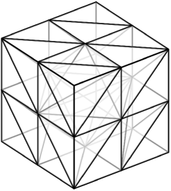
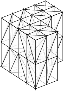
Figure 8. Initial triangulations of the cube and the tensor product L-shaped domain.

The $H^{1}$ errors and the $L^{2}$ errors of the velocity $u$ are depicted in the convergence history plot in Figure 9. The $H^{1}$ errors show convergence rates of $\mathcal{O}(h)$ for all methods, while the convergence rates of the $L^{2}$ errors of all methods are near $\mathcal{O}(h^{2})$ with a slightly larger convergence rate for $V_{2,D}$.

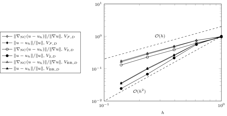
Figure 9. Convergence history plot for the example from Subsection 5.1

5.2. Smooth solution on the cube, II

This subsection considers the smooth exact solution

$$u (x)=\begin{pmatrix}10x_{1}x_{2}^{4}+10x_{1}x_{3}^{4}-4x_{1}^{5}\\ 10x_{2}x_{1}^{4}+10x_{2}x_{3}^{4}-4x_{2}^{5}\\ 10x_{3}x_{1}^{4}+10x_{3}x_{2}^{4}-4x_{3}^{5}\end{pmatrix},$$

$$p (x)=-60x_{1}^{2}x_{2}^{2}-60x_{1}^{2}x_{3}^{2}-60x_{2}^{2}x_{3}^{2}+20x_{1}^{4}+20x_{2}^{4}+20x_{3}^{4}$$

on the cube $\Omega=(-1,1)^{3}$ with Neumann boundary $\Gamma_{N}=(0,1)^{2}\times\{-1\}$ and Dirichlet boundary $\Gamma_{D}=\partial\Omega\setminus\Gamma_{N}$. As in subsection 5.1, the solutions to (2.1) with $V_{h,D}=V_{2,D}$ and $V_{h,D}=V_{\mathcal{F},D}$ and the solution of the Bernardi-Raugel FEM for the right-hand side $f$ and $g$ given by the exact solution are computed on a sequence of red-refined triangulations. The initial triangulation is depicted in Figure 8. The $H^{1}$ errors and the $L^{2}$ errors of the velocity $u$ are depicted in the convergence history plot in Figure 10. The $H^{1}$ errors show convergence rates of $\mathcal{O}(h)$ for all methods, while the convergence rates of the $L^{2}$ errors of both nonconforming methods are slightly worse than $\mathcal{O}(h^{2})$. The convergence rate of the $L^{2}$ error for the Bernardi-Raugel FEM seems to be larger than that of the two nonconforming FEMs.

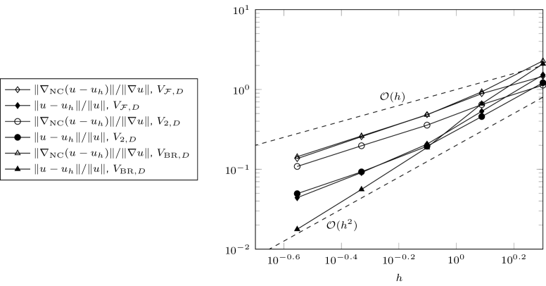
Figure 10. Convergence history plot for the example from Subsection 5.2

5.3. Smooth solution on the cube, III

This subsection considers the smooth exact solution

$$u(x) =\begin{pmatrix}2x_{2}x_{3}(x_{1}^{2}-1)^{2}(x_{2}^{2}-1)(x_{3}^{2}-1)\\ -x_{1}x_{3}(x_{1}^{2}-1)(x_{2}^{2}-1)^{2}(x_{3}^{2}-1)\\ -x_{1}x_{2}(x_{1}^{2}-1)(x_{2}^{2}-1)(x_{3}^{2}-1)^{2}\end{pmatrix},$$

$$p(x) =x_{1}x_{2}x_{3}$$

on the cube $\Omega=(-1,1)^{3}$ with Neumann boundary $\Gamma_{N}=(0,1)^{2}\times\{-1\}$ and Dirichlet boundary $\Gamma_{D}=\partial\Omega\setminus\Gamma_{N}$. As in subsections 5.1–5.2, the solutions to (2.1) with $V_{h,D}=V_{2,D}$ and $V_{h,D}=V_{\mathcal{F},D}$ and the solution of the Bernardi-Raugel FEM for the right-hand side $f$ and $g$ given by the exact solution are computed on a sequence of red-refined triangulations. The initial triangulation is depicted in Figure 8. The $H^{1}$ errors and the $L^{2}$ errors of the velocity $u$ are depicted in the convergence history plot in Figure 11. The $H^{1}$ errors show convergence rates slightly worse than $\mathcal{O}(h)$ for all three methods. As the convergence rate still increases under the considered refinements, it is suggested that the asymptotic regime is not reached at this point. The convergence rates of the $L^{2}$ errors of all three methods are $\mathcal{O}(h^{2})$ for all methods.

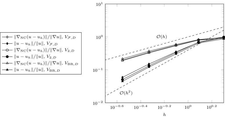
Figure 11. Convergence history plot for the example from Subsection 5.3

5.4. Singular solution on the 3D tensor product L-shaped domain

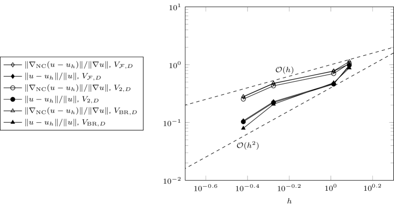
Figure 12. Convergence history plot for the example from Subsection 5.4

This subsection considers the tensor product L-shaped domain

$$\Omega=\left((-1,1)^{2}\setminus([0,1]\times[-1,0])\right)\times(-1,1)$$

with $\Gamma_{N}:=\{1\}\times(0,1)\times(-1,1)$ and exact solution

$$u(x_{1},x_{2},x_{3})=\operatorname{curl}\begin{pmatrix}(1-x_{3}^{2})^{2}u_{\mathrm{Gr}}(x_{1},x_{2})\\ \cos(\pi x_{3})u_{\mathrm{Gr}}(x_{1},x_{2})\\ x_{3}u_{\mathrm{Gr}}(x_{1},x_{2}),\end{pmatrix}\qquad\text{and}\qquad p=0,$$

where $u_{\mathrm{Gr}}$ is the singular solution for the 2d plate problem on the L-shaped domain from [Gri92, p. 107] and reads in polar coordinates

$$u(r,\theta)=(r^{2}\cos^{2}\theta-1)^{2}(r^{2}\sin^{2}\theta-1)^{2}\,r^{1+\alpha}\,g(\theta).$$

Here, $\alpha:=0.544483736782464$ is a noncharacteristic root of $\sin^{2}(\alpha\omega)=\alpha^{2}\sin^{2}(\omega)$ for $\omega:=3\pi/2$ and

$$g(\theta) =\left[\frac{\sin((\alpha-1)\omega)}{\alpha-1}-\frac{\sin((\alpha+1)\omega)}{\alpha+1}\right](\cos((\alpha-1)\theta)-\cos((\alpha+1)\theta)$$

$$\qquad-\left[\frac{\sin((\alpha-1)\theta)}{\alpha-1}-\frac{\sin((\alpha+1)\theta)}{\alpha+1}\right](\cos((\alpha-1)\omega)-\cos((\alpha+1)\omega).$$

The right-hand side data $f$ and $g$ are chosen according to the exact solution. The initial triangulation is depicted in Figure 8. The $H^{1}$ and $L^{2}$ errors are plotted in Figure 12 against the mesh-size. Although the exact solution is not in $H^{2}(\Omega)$, the convergence rate of the $H^{1}$ errors for all three methods seems to be $\mathcal{O}(h)$, at least in a pre-asymptotic regime. This is in agreement with numerical experiments in 2d and 3d for the plate problem, where the reduced convergence rate can only be seen in the regime of very fine meshes. The $L^{2}$ errors show convergence rates slightly smaller than $\mathcal{O}(h^{2})$ for the three considered methods, but the Bernardi-Raugel FEM seems to have a slightly better convergence rate than the two nonconforming FEMs.

References

- [Arn93] Douglas N. Arnold. On nonconforming linear-constant elements for some variants of the Stokes equations. Istit. Lombardo Accad. Sci. Lett. Rend. A, 127(1):83–93 (1994), 1993.
- [BBF13] D. Boffi, F. Brezzi, and M. Fortin. Mixed Finite Element Methods and Applications, volume 44 of Springer Series in Computational Mathematics. Springer, Heidelberg, 2013.
- [BCGG12a] D. Boffi, N. Cavallini, F. Gardini, and L. Gastaldi. Local mass conservation of Stokes finite elements. J. Sci. Comput., 52(2):383–400, 2012.
- [BCGG12b] D. Boffi, N. Cavallini, F. Gardini, and L. Gastaldi. Stabilized Stokes elements and local mass conservation. Boll. Unione Mat. Ital. (9), 5(3):543–573, 2012.
- [BCGG14] S. Badia, R. Codina, T. Gudi, and J. Guzmán. Error analysis of discontinuous Galerkin methods for the Stokes problem under minimal regularity. IMA J. Numer. Anal., 34(2):800–819, 2014.
- [Bof97] D. Boffi. Three-dimensional finite element methods for the Stokes problem. SIAM J. Numer. Anal., 34(2):664–670, 1997.
- [BR85] C. Bernardi and G. Raugel. Analysis of some finite elements for the Stokes problem. Math. Comp., 44(169):71–79, 1985.
- [Bre03] S.C. Brenner. Poincaré-Friedrichs inequalities for piecewise functions. SIAM J. Numer. Anal., 41(1):306–324, 2003.
- [Bre04] S.C. Brenner. Korn’s inequalities for piecewise vector fields. Math. Comp., 73(247):1067–1087, 2004.
- [BS08] Susanne C. Brenner and L. Ridgway Scott. The Mathematical Theory of Finite Element Methods, volume 15 of Texts in Applied Mathematics. Springer Verlag, New York, Berlin, Heidelberg, 3 edition, 2008.
- [Car05] C. Carstensen. A unifying theory of a posteriori finite element error control. Numer. Math., 100(4):617–637, 2005.
- [CH07] C. Carstensen and J. Hu. A unifying theory of a posteriori error control for nonconforming finite element methods. Numer. Math., 107(3):473–502, 2007.
- [CKPS15] C. Carstensen, K. Köhler, D. Peterseim, and M. Schedensack. Comparison results for the Stokes equations. Appl. Numer. Math., 95:118–129, 2015. Published online.
- [CR73] M. Crouzeix and P.-A. Raviart. Conforming and nonconforming finite element methods for solving the stationary Stokes equations. I. Rev. Française Automat. Informat. Recherche Opérationnelle Sér. Rouge, 7(R-3):33–75, 1973.
- [CS15] C. Carstensen and M. Schedensack. Medius analysis and comparison results for first-order finite element methods in linear elasticity. IMA J. Numer. Anal., 35(4):1591–1621, 2015.
- [FM90] Richard S. Falk and Mary E. Morley. Equivalence of finite element methods for problems in elasticity. SIAM J. Numer. Anal., 27(6):1486–1505, 1990.
- [GN14] Johnny Guzmán and Michael Neilan. Conforming and divergence-free Stokes elements on general triangular meshes. Math. Comp., 83(285):15–36, 2014.
- [Gri92] P. Grisvard. Singularities in boundary value problems, volume 22 of Recherches en Mathématiques Appliquées [Research in Applied Mathematics]. Masson, Paris; Springer-Verlag, Berlin, 1992.
- [Gud10] T. Gudi. A new error analysis for discontinuous finite element methods for linear elliptic problems. Math. Comp., 79(272):2169–2189, 2010.
- [HMS14] Jun Hu, Rui Ma, and ZhongCi Shi. A new a priori error estimate of nonconforming finite element methods. Sci. China Math., 57(5):887–902, 2014.
- [KS95] R. Kouhia and R. Stenberg. A linear nonconforming finite element method for nearly incompressible elasticity and Stokes flow. Comput. Methods Appl. Mech. Engrg., 124(3):195–212, 1995.
- [NS16] M. Neilan and D. Sap. Stokes elements on cubic meshes yielding divergence-free approximations. Calcolo, 53(3):263–283, 2016.
- [Sch17] M. Schedensack. Mixed finite element methods for linear elasticity and the Stokes equations based on the Helmholtz decomposition. ESAIM Math. Model. Numer. Anal., 51(2):399–425, 2017.
- [Ste87] R. Stenberg. On some three-dimensional finite elements for incompressible media. Comput. Methods Appl. Mech. Engrg., 63(3):261–269, 1987.
- [Ste90] Rolf Stenberg. A technique for analysing finite element methods for viscous incompressible flow. Internat. J. Numer. Methods Fluids, 11(6):935–948, 1990. The Seventh International Conference on Finite Elements in Flow Problems (Huntsville, AL, 1989).
- [Ver13] Rüdiger Verfürth. A posteriori error estimation techniques for finite element methods. Numerical Mathematics and Scientific Computation. Oxford University Press, Oxford, 2013.
- [Zha05] S. Zhang. A new family of stable mixed finite elements for the 3D Stokes equations. Math. Comp., 74(250):543–554, 2005.