Adiabatic elimination of inertia of the stochastic microswimmer driven by $\alpha-$stable noise

Abstract

We consider a microswimmer that moves in two dimensions at a constant speed and changes the direction of its motion due to a torque consisting of a constant and a fluctuating component. The latter will be modeled by a symmetric Lévy-stable ($\alpha$-stable) noise. The purpose is to develop a kinetic approach to eliminate the angular component of the dynamics in order to find a coarse grained description in the coordinate space. By defining the joint probability density function of the position and of the orientation of the particle through the Fokker-Planck equation, we derive transport equations for the position-dependent marginal density, the particle’s mean velocity and the velocity’s variance. At time scales larger than the relaxation time of the torque $\tau_{\phi}$ the two higher moments follow the marginal density, and can be adiabatically eliminated. As a result, a closed equation for the marginal density follows. This equation which gives a coarse-grained description of the microswimmer’s positions at time scales $t\gg\tau_{\phi}$, is a diffusion equation with a constant diffusion coefficient depending on the properties of the noise. Hence, the long time dynamics of a microswimmer can be described as a normal, diffusive, Brownian motion with Gaussian increments.

I Introduction

A popular class of models used to describe active particles assumes that the particles’ motion remains at a constant speed. In these models the Newtonian equations of motion for an active particle reduce to the consideration of its orientational dynamics.

The direction of motion changes due to a torque,which has a constant as well as fluctuating contributions, modeled as noise. The noise may appear due to external forces acting on the particle, due to interaction with other particles, or by consequences of the nature of the particle’s internal propulsive mechanism romanczuk2011 ; gromann2016 ; mijalkov2013 ; volpe2014 ; geiseler2016 ; geiseler2016kramers ; patch2017 ; debnath ; btenhagen ; babel . The introduction of the constant torque is necessary to be able to describe situation like the ones found in some bacteria as Escherichia coli DiLuzio ; Hill , and in spermatozoaWolley ; Riedel ; teeffelen ; friedrich which are known to swim in circles. Artificial Janus particles Dhar ; Kudrolli ; kummel and particles in drift chambers astro can also move in circles when the symmetry is broken.

Active particles without noise are sometimes called microswimmers. If random torques are present, as in our considered cased, we call them stochastic microswimmers. Previous works on stochastic microswimmers have investigated the effect of random torques modeled by a Gaussian noise weber_sokolov_lsg , by a dichotomous Markov process Weber , and also by $\alpha$-stable noetl_sokolov_lsg:2017 noise. These investigations have focused on calculating the mean squared displacements (MSD) in dependence on the parameters characterizing the noise. As a result it was shown that for all these different kinds of angular noise the particles exhibit ballistic motion at short time scales and diffusive motion at longer times. The ballistic motion is caused by the inertia of the swimmer, i.e. due to the fact that the particle remembers for a certain time interval the direction it has currently moved in. However, for longer times, i.e. at time scales larger than the relaxation time of the orientation, this orientational memory fades out, and the normal diffusive behavior sets on.

Such a crossover between ballistic and diffusive motion is best known for normal (i.e. non-active) Brownian motion langevin ; Becker52 ; Hwalisz ; Milster . The particle’s motion is described by the joint probability density in the phase space, i.e. for the particle’s velocity and position. The coarse-grained description for the position variables only leads to a diffusion equation. Therein, the velocity of the particle as a dynamical variable has been eliminated. This coarse-grained description is valid at time scales $\Delta t\gg\tau_{v}$ and at length scales $|\Delta\vec{r}|\gg l_{v}=\tau_{v}\sqrt{k_{\rm B}T/m}$. Therein $\tau_{v}=m/\gamma$ is the velocity relaxation time and $l_{v}$ is the brake path, or persistence length of Brownian motion, with $m$ being the mass of the particle and $\gamma$ the particle’s friction coefficient. In situations where $\tau_{v}$ is small the dynamics is often referred to as an overdamped dynamics.

For Brownian motion, there exists a vast literature which considers the elimination of inertia at larger time and length scales. Already Kramers in his seminal work Kramers found an elegant way to eliminate the velocity. Using the factorizing properties of the Fokker-Planck operator, he was able to derive the diffusion equation for the marginal probability density $\rho(\mathbf{r},t)$ (see also Becker52 ). Later on, many other approaches have been formulated, including the projection operator formalism and approaches which adiabatically eliminate variables haken ; gardiner ; gardiner:82 ; ucna ; lsg_talkner ; sancho .

Here, we seek for the foundation of the diffusive motion of the microswimmer by adiabatic elimination of the angular inertia. We will derive a coarse-grained description of the particle’s motion at time and length scales where the angular memory fades out, and calculate the distribution of its displacements. To the best of our knowledge, such an elimination procedure for a stochastic microswimmer has not been previously considered in detail. The case in which Gaussian white noise models the torque was elaborated only recently. Therein, the angular inertia was eliminated in the corresponding Langevin equation, and the coarse grained Langevin equations of the diffusing microswimmer were derived and discussed Milster . For sake of completeness, we show in Appendix A the elimination with torque and Gaussian white noise, from the Langevin equations.

In the present work we will study the broader situation, and consider a model for a stochastic microswimmer in which orientational changes are due to a combination of a constant torque and of random fluctuations described by an $\alpha$-stable noise. We are interested in obtaining the coarse grained dynamical description in the coordinate space. Surprisingly, despite the Lévy nature of the noise in the angular variable, the coarse grained dynamics is found to be modeled through Gaussian white noise acting in the coordinate space. Thus, the long time behavior can be universally described as Brownian motion.

We have been unable to perform this elimination on the level of the Langevin equation. Due to the heavy-tailed nature of the increments of the $\alpha$-stable noise, the moments needed in the corresponding derivation do not exist. Here we will use a kinetic approach which, for the case of Gaussian white noise, has been developed in Milster . This approach uses the transport equations for the first three moments of the velocity components. These velocity components are expressed by the cosine and sine of the orientation. Since these are bounded functions, their mean values exist even for the case that the angular dynamics is due to Lévy noise.

In section II we introduce the model and present the results of simulations of the stochastic microswimmer. In section III we formulate the Fokker-Planck equation for the joint probability density function (pdf) of the orientation and the position of the microswimmer in two dimensional coordinate space. We then derive equations for the reduced moments of this pdf, which are the marginal pdf of the position of the particle, the average velocity components, and their variances. By expressing higher moments through the first three, these equations represent an approximation of the dynamics in the position space. In section IV we discuss the procedure of the adiabatic elimination of the velocity variables. At time scales larger than the crossover time $\tau_{\phi}$, we assume that the variance of the velocity follows the marginal density and the velocities squared. Further on, we assume that the mean velocities follow the marginal density, and eliminate both the velocity’s first and second moment. As a result we obtain a closed equation for the marginal position-dependent density. This is a diffusion equation having as solution the Gaussian distributions of independent spatial displacements. The diffusion coefficient characterizing the linear growth of the variance of these displacements is a constant that depends on the parameters characterizing the $\alpha$-stable noise.

II The Model

We consider a microswimmer in two dimensions whose position is given by a vector $\vec{r}=\left(x(t),y(t)\right)$. The position space is unbounded. The swimmer starts at time $t_{0}=0$ at position $\vec{r}_{0}=(x_{0}=0,y_{0}=0)$ and has a constant speed $v_{0}>0$ but the actual heading is given by the angle $\phi(t)\in[0,2\pi)$, so that the dynamics is described by a set of equations

$$\frac{\text{d}\vec{r}}{\text{d}t}=\vec{v}=v_{0}\begin{pmatrix}\cos\phi(t)\\ \sin\phi(t)\end{pmatrix}\,,$$ (1)

$$\frac{\text{d}\phi}{\text{d}t}=\Omega+\frac{\sigma}{v_{0}}\xi(t)\,.$$ (2)

Here $\Omega$ is a time-independent torque, and the noise $\xi(t)$ is assumed to be white, $\alpha$-stable and symmetric feller , with noise strength $\sigma$.

The term $\alpha-$stable (Lévy stable) refers to the fact that the sum of random variables following a stable distribution follows the same probability distribution up to a rescaling and a re-centering. The increments of the noise are independent. The commonly used Gaussian noise (corresponding to $\alpha=2$) is one example of such stable white noises. The parameter $\alpha$ is the Lévy stability index, and characterizes the tails of the probability distribution. Decreasing $\alpha$ leads to larger sudden changes in the direction of motion. For values of $\alpha<2$ the tails of the corresponding probability distributions become heavier, and the corresponding random variables show more outliers. Distributions with $\alpha<2$ have infinite variance and for $\alpha\leq 1$ even the first moment no longer exist.

Such non-Gaussian noise distributions are quite useful to describe the motion of entities which behave like hunted rabbits or antelopes. Typical trajectories of such a running animal with rapid turning behavior are not best described by Gaussian increments. The motion of a particle under such conditions is better characterized by a run and tumble behavior runandtumble1 ; runandtumble2 with fast periods of tumbling. Recent experiments on motions of fruit flies Kim2017 ; Jundi2017 have reported similar trajectories with rapid changes.

The active particles described by the set of equations (1), (2) perform a ballistic motion on a short time-scale $t\ll\tau_{\phi}$ noetl_sokolov_lsg:2017 with

$$\tau_{\phi}=\left(\frac{v_{0}}{\sigma}\right)^{\alpha},$$ (3)

being the relaxation time and with the persistence length $l_{p}=v_{0}\tau_{\phi}$. At longer times $t\gg\tau_{\phi}$ and at distances $|vec{r}|\gg l_{p}$ the motion becomes diffusive with the effective diffusion coefficient

$$D_{\text{eff}}=\frac{v_{0}^{2}}{2}\frac{\tau_{\phi}}{1+\left(\Omega\tau_{\phi}\right)^{2}}.$$ (4)

The diffusion coefficient and the relaxation time were calculated in noetl_sokolov_lsg:2017 using the Green-Kubo relation.

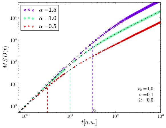
Figure 1: Mean squared displacement of the stochastic microswimmer for various values of $\alpha$. The crossover between ballistic and diffusive behavior takes places at indicated transition times. The transition times equal the relaxation times of the angular dynamics $\tau_{\phi}$ and depend on the choice of $\alpha$. The broken line corresponds to the MSD calculated using the Green-Kubo relation in noetl_sokolov_lsg:2017 .

The mean squared displacement as a function of time is shown in Figure 1 for various values of $\alpha$. Due to the angular inertia, or memory, the motion is ballistic for times smaller $t\ll\tau_{\phi}$ and at times $t\gg\tau_{\phi}$ becomes diffusive with the diffusion coefficient $D_{\text{eff}}$ given by eq.(4). In the figures the crossover time, being the relaxation time of the angular dynamics, increases with $\alpha$ when other parameters are kept fixed.

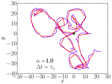
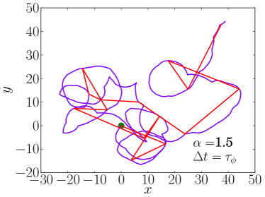
Figure 2: Sample trajectories of the stochastic microswimmer with constant speed for $\alpha=1$ (left) and $\alpha=1.5$ (right). Trajectories start at $(0,0)$, marked as green dot. The blue trajectories are the persistent paths. Their coarse grained dynamics are shown in red and taken in sampling intervals of $\Delta t=\tau_{\phi}$. Other parameters $v_{0}=1.0$, $\sigma=0.1$ and $\Omega=0.1$. The trajectories contain a total simulation time of t=500.

Figure 2 shows sample trajectories of stochastic microswimmers for $\alpha=1$ (left panel) and for $\alpha=1.5$ (right panel). The blue lines show simulated paths plotted with a time increment $\Delta t=0.1$ much smaller than the relaxation time. One can see motion over almost straight lines interrupted by sharp turns. For lower values of $\alpha$, here $\alpha=1$, trajectories become rather smooth occasionally interrupted by sharp turns. In contrast, the red paths represent the coarse grained dynamics of the blue trajectories sampled with $\Delta t=\tau_{\phi}$ (compare Eq.(3)). At this large time scale the motion is just at the crossover time, beyond which the motion starts to be diffusive with independent increments and statistically indistinguishable from Brownian motion.

For all values of $\alpha$, an initial angle $\phi(t_{0}=0)=\phi_{0}$ is forgotten after the relaxation time $\tau_{\phi}$ has elapsed. Moreover, for long enough times $t\gg\tau_{\phi}$ the angular transition probability density $Q=Q(\phi,t|\phi_{0},t_{0})$ becomes uniform. This follows from the corresponding Fokker-Planck-Equation (FPE) for $Q$ which decouples from the coordinate dynamics since Eq.(2) is autonomous. This FPE reads Ditlevsen ; Schertzer

$$\frac{\partial}{\partial t}\,Q(\phi,t|\phi_{0},t_{0})\,=\,-\,\frac{\partial}{\partial\phi}\,\Omega Q\,+\,\frac{1}{\tau_{\phi}}\frac{\partial^{\alpha}}{\partial|\phi|^{\alpha}}\,Q\,,$$ (5)

with the $\alpha$-th symmetric Riesz-Weyl fractional derivative

$$\frac{\partial^{\alpha}}{\partial|\phi|^{\alpha}}\,Q(\phi,t|\phi_{0},t_{0})\,=\,-\,\frac{1}{2\pi}\,\int_{-\infty}^{\infty}\,{\rm d}k\,e^{-ik\phi}\,|k|^{\alpha}\,Q(k,t|\phi_{0},t_{0})\,,$$ (6)

where

$$Q(k,t|\phi_{0},t_{0})\,=\,\int_{-\infty}^{\infty}\,{\rm d}\phi e^{ik\phi}\,Q(\phi,t|\phi_{0},t_{0})\,,$$ (7)

is the Fourier transform of the transition probability density with respect to the angular variable $\phi$. The solution to eq. (5) is

$$Q(\phi,t|\phi_{0},t_{0}=0)=\frac{1}{\pi}\left(\frac{1}{2}+\sum_{n=1}^{\infty}\cos\left(n(\phi-\phi_{0}-\Omega t)\right)e^{-\frac{n^{\alpha}t}{\tau_{\phi}}}\right),$$ (8)

which takes into account the $2\pi$-periodicity of the angular variable and the initial condition $\phi(t=0)=\phi_{0}$, i.e. $Q(\phi,t=0|\phi_{0},0)=\delta(\phi-\phi_{0})$. The case $\alpha=2$ corresponds to a Gaussian white noise. For times $t\gg\tau_{\phi}$ the probability density to find a specific angle becomes constant $1/(2\pi)$ for all symmetric $\alpha-$stable noise types. Note that for the slowest mode the only parameter which depends on the noise type is the relaxation time $\tau_{\phi}$. The flattening of the angular distribution is the key feature that allows the description of our active particles as Brownian particles in the long-time limit.

As already reported in noetl_sokolov_lsg:2017 , numerical simulations show a Gaussian distribution of displacements at times larger the relaxation time $t\gg\tau_{\phi}$ for all considered noise types. In polar coordinates $(r,\varphi)$ the displacement’s distribution is independent from the spatial angle $\varphi$ at this time scale. For simplicity, we take the origin as the initial position, i.e. $x_{0}=0,y_{0}=0$. The distribution of the distance to the origin $r(t)=\sqrt{x^{2}(t)+y^{2}(t)}$ is given by the Rayleigh distribution. This is to be expected since for longer time increments of the heading become uncorrelated, and the step length is finite.

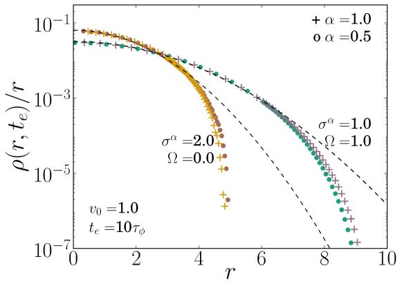
Figure 3: Simulation results for the radial displacement distribution divided by $r$, i.e. $\rho(r,t_{e}|0,0)/r$ taken at time $t_{e}=10\tau_{\phi}$. Results are shown for two different values of $\alpha$ indicated by circles ($\alpha=0.5$) and crosses ($\alpha=1.0$). Results are for two different noise intensities with indicated values. Note, due to the dependence of $\tau_{\phi}$ on $\alpha$ the brown and green results have been taken at different end time $t_{e}$. Black dashed line corresponds to a Rayleigh distribution with mean squared displacement $\langle r^{2}\rangle=4D_{\text{eff}}t$ and $D_{\text{eff}}$ from (4). Other parameters are given in the figure.

Figure 3 shows simulation results for the radial displacement distribution divided by $r$, i.e. for $\rho(r,t_{e}|0,0)/r$, after time $t_{e}=10\tau_{\phi}$. Black dashed line corresponds to a Rayleigh distribution with mean squared displacement $\langle\,r^{2}\,\rangle=4D_{\text{eff}}t$ where $D_{\text{eff}}$ is Eq. (4). The Rayleigh distribution coincides well with the simulations up to $r\approx 0.7v_{0}t_{e}$. When $r>>0.7v_{0}t_{e}$ the inertia and the constant kinetic energy of the microswimmer cause deviations.

III Kinetic approach of eliminating the angular memory

In this section we will follow a kinetic approach based on the Fokker-Planck equation, similar to the approach used in Milster for active particles with Gaussian white noise. Here we consider the broader class of symmetric $\alpha-$stable noises. In addition, we consider the effects of the constant torque, a physical situation often met for motile particles.

The kinetic approach is based on the first three reduced coordinate-dependent moments of the velocity, which we will soon define. In our two dimensional situation with constant speed the reduced moments are obtained by averaging over the heading $\phi$. Afterwards as in kinetic theory, the spatio-temporal evolution is determined by the transport equations for the marginal probability density, components of the the average velocities and the variances of the velocity. In these equations, we will adiabatically eliminate higher moments. This enables us to approximate the variances and mean velocity in order to find a closed description for the dynamics of active particle considered.

Associated with the given Langevin equations (1),(2) is the following FPE Ditlevsen ; Schertzer :

$$\frac{\partial}{\partial t}P(x,y,\phi,t|x_{0},y_{0},\phi_{0},t_{0})=-\vec{v}\cdot\nabla P-\frac{\partial}{\partial\phi}\Omega P+\frac{1}{\tau_{\phi}}\frac{\partial^{\alpha}}{\partial|\phi|^{\alpha}}P,$$ (9)

$\vec{v}=(v_{x},v_{y})^{T}$ for the transition pdf $P=P(x,y,\phi,t|x_{0},y_{0},\phi_{0},t_{0})$. The aforementioned reduced moments are the marginal probability density $\rho(x,y,t)$, the mean velocity components $u_{i}(x,y,t)$ and the variances $\sigma_{ij}(x,y,t)$

$$\rho(x,y,t)=\int_{0}^{2\pi}P(x,y,\phi,t)d\phi$$ (10)

$$\rho(x,y,t)u_{i}(x,y,t)=\int_{0}^{2\pi}v_{i}P(x,y,\phi,t)d\phi$$ (11)

$$\rho(x,y,t)\sigma_{ij}^{2}(x,y,t)=\int_{0}^{2\pi}(v_{i}-u_{i}(x,y,t))(v_{j}-u_{j}(x,y,t))P(x,y,\phi,t)d\phi$$ (12)

with $i,j\in[x,y]$. We omitted for readability the conditions of $P$ in the equations .

The application of this kinetic approach to our model is straightforward since such properties as the non-existence of higher moments $\langle\phi^{n}\rangle$ (for $n\geq 2$ with $\alpha<2$ and for $n\geq 1$ in case of $\alpha\leq 1$) do not matter. While these moments might not exist, the mathematical expectations of the periodic functions $\langle\cos(\phi)\rangle$,$\langle\sin(\phi)\rangle$ and their powers stay finite, see Appendix B for details.

The transport equations for the corresponding moments are derived by differentiating equations (10),(11),(12) with respect to time and using the Fokker-Planck equation (9) which has to be integrated over the angle $\phi$. As a result, we obtain the continuity equation

$$\frac{\partial}{\partial t}\rho\,=\,-\frac{\partial}{\partial x}\rho u_{x}\,-\,\frac{\partial}{\partial y}\rho u_{y}\,,$$ (13)

and the transport equation for the momentum

$$\frac{\partial}{\partial t}\rho u_{i}=-\left(\frac{\partial}{\partial x_{i}}\rho(u_{i}^{2}+\sigma_{ii}^{2})+\frac{\partial}{\partial x_{j}}\rho(u_{i}u_{j}+\sigma_{ij}^{2})\right)-a_{i}\Omega\rho u_{j}-\frac{1}{\tau_{\phi}}\rho u_{i}\,.$$ (14)

Differentiating (12) with respect to time, we obtain the balance equations for the variances

$$\frac{\partial}{\partial t}\rho\left(u_{i}^{2}+\sigma_{ii}^{2}\right)=A_{ii}-\frac{2^{\alpha}}{\tau_{\phi}}\rho\left(u_{i}^{2}+\sigma_{ii}^{2}-\frac{v_{0}^{2}}{2}\right)-a_{i}2\Omega\rho\left(u_{i}u_{j}+\sigma_{ij}^{2}\right)\,,$$ (15)

and, respectively, for the covariance;

$$\frac{\partial}{\partial t}\rho\left(u_{i}u_{j}+\sigma_{ij}^{2}\right)=A_{ij}-\frac{2^{\alpha}}{\tau_{\phi}}\rho\left(u_{i}u_{j}+\sigma_{ij}^{2}\right)+\Omega\rho\left(a_{i}\left(u_{i}^{2}+\sigma_{ii}^{2}\right)+a_{j}\left(u_{j}^{2}+\sigma_{jj}^{2}\right)\right)\,.$$ (16)

Notably, the specific noise distributions of the $\alpha$-stable noise sources enter all transport equations only through constant parameters, i.e. through the value of $2^{\alpha}$ and through $\tau_{\phi}$. In the equations above (14),(15) and (16) the indices run over $i,j=x,y$ and $i\neq j$. Also, we do not sum over a repeated indices. Further on, $a_{x}=1$, $a_{y}=-1$ and the appearing higher moments $A_{ij}$ take the following form:

$$\begin{split}A_{xx}=-\frac{\partial}{\partial x}\int_{0}^{2\pi}v_{0}^{3}\cos^{3}(\phi)P(x,y,\phi,t)d\phi-\frac{\partial}{\partial y}\int_{0}^{2\pi}v_{0}^{3}\cos^{2}(\phi)\sin(\phi)P(x,y,\phi,t)d\phi\end{split}$$ (17)

$$\begin{split}A_{yy}=-\frac{\partial}{\partial x}\int_{0}^{2\pi}v_{0}^{3}\cos(\phi)\sin^{2}(\phi)P(x,y,\phi,t)d\phi-\frac{\partial}{\partial y}\int_{0}^{2\pi}v_{0}^{3}\sin^{3}(\phi)P(x,y,\phi,t)d\phi\end{split}$$ (18)

$$\begin{split}A_{xy}=-\frac{\partial}{\partial x}\int_{0}^{2\pi}v_{0}^{3}\cos^{2}(\phi)\sin(\phi)P(x,y,\phi,t)d\phi-\frac{\partial}{\partial y}\int_{0}^{2\pi}v_{0}^{3}\cos(\phi)\sin^{2}(\phi)P(x,y,\phi,t)d\phi\end{split}$$ (19)

IV Adiabatic elimination

We will now adiabatically eliminate the angular inertia, or angular memory from the transport equations (15). In contrast to the case of Brownian particles, the relaxation time does depend on the noise intensity, $\tau_{\phi}\propto 1/\sigma^{\alpha}$ . Hence, large noise intensity $\sigma$ corresponds to larger angular variability, and therefore to faster relaxation. We will consider the limit of large noise meaning that the relaxation time $\tau_{\phi}$ can be considered as small compared to the time scale of observation. Multiplication of (15) and (16) by $\tau_{\phi}/2^{\alpha}$ yields an expression that allows us to neglect the time derivatives and the higher moments in $A_{ii}$ and $A_{ij}$ in these equations.

We retain terms with $\Omega\tau_{\phi}$ since $\Omega$ could be large in contrast to the derivatives of higher moments which are considered small.

Therefore, we neglect the temporal derivatives in the equations for variances and covariances. Also the influence of the higher moments disappears in the limit of small $\tau_{\phi}$. The variances as well as the covariances then follow the other time dependent moments. Starting from Eq.(15) we derive the following two equations:

$$\rho\left(u_{x}^{2}+\sigma_{xx}^{2}\right)\,+\,2\Omega\frac{\tau_{\phi}}{2^{\alpha}}\,\rho\left(u_{x}u_{y}+\sigma_{xy}^{2}\right)\,=\,\rho\frac{v_{0}^{2}}{2}\,+\,\mathcal{O}(\tau_{\phi})$$ (20)

$$\rho\left(u_{y}^{2}+\sigma_{yy}^{2}\right)\,-\,2\Omega\frac{\tau_{\phi}}{2^{\alpha}}\,\rho\left(u_{x}u_{y}+\sigma_{xy}^{2}\right)\,=\,\rho\frac{v_{0}^{2}}{2}\,+\,\mathcal{O}(\tau_{\phi}).$$ (21)

Respectively, using Eq. (16) we obtain

$$\Omega\frac{\tau_{\phi}}{2^{\alpha}}\rho\,\left(u_{y}^{2}+\sigma_{yy}^{2}-u_{x}^{2}-\sigma_{xx}^{2}\right)\,+\,\rho\left(u_{x}u_{y}+\sigma_{xy}^{2}\right)\,=\,0\,+\,\mathcal{O}(\tau_{\phi})\,.$$ (22)

The solution of this set of three bi-linear equations is:

$$u_{i}u_{j}+\sigma_{ij}^{2}\,=\,\delta_{ij}\frac{v_{0}^{2}}{2}\,+\,\mathcal{O}(\tau_{\phi})\,.$$ (23)

This solution is a kind of equipartition theorem for the two terms in the kinetic energy and is valid at times larger the relaxation time.

Next we consider the momentum balance, Eq. (14). Assuming again $t\gg\tau_{\phi}$ will allow us again to neglect the time derivative. Further on, inserting therein the values of the (co-)variances as given by Eq. (23) yields for $i,j=x,y;i\neq j$

$$\rho\left(u_{i}\,+\,a_{i}\Omega\tau_{\phi}u_{j}\right)\,=\,\tau_{\phi}\frac{v_{0}^{2}}{2}\,\frac{\partial}{\partial x_{i}}\rho\,+\,\mathcal{O}(\tau_{\phi}),$$ (24)

meaning that the two first momenta follow quickly the marginal density. Like $\Omega$, the velocity $v_{0}$ is arbitrary, and therefore $v_{0}^{2}\tau_{\phi}$ is not negligible in general (see Eq. (4)). The solution with respect to the components of the mean flux can be easily obtained. It gives

$$\rho u_{x}\,=\,-\,\frac{\tau_{\phi}}{1+\Omega^{2}\tau_{\phi}^{2}}\frac{v_{0}^{2}}{2}\,\left(\frac{\partial}{\partial x}\rho\,-\,\Omega\tau_{\phi}\,\frac{\partial}{\partial y}\rho\right)\,+\,\mathcal{O}(\tau_{\phi})\,,$$

$$\rho u_{y}\,=\,-\,\frac{\tau_{\phi}}{1+\Omega^{2}\tau_{\phi}^{2}}\frac{v_{0}^{2}}{2}\,\left(\Omega\tau_{\phi}\,\frac{\partial}{\partial x}\rho\,+\,\frac{\partial}{\partial y}\rho\right)\,+\,\mathcal{O}(\tau_{\phi})\,.$$ (25)

Eventually, we put these expressions for the mean momenta into the continuity equation (13). Hence, up to first order of $\tau_{\phi}$ we derive the evolution equation for the marginal probability density $\rho(x,y,t)$ of a stochastic microswimmer driven by $\alpha$-stable noise. It is the well known diffusion equation reading

$$\frac{\partial}{\partial t}\rho(x,y,t)\,=\,D_{\rm eff}\left(\frac{\partial^{2}}{\partial x^{2}}+\frac{\partial^{2}}{\partial y^{2}}\right)\rho\,+\,\mathcal{O}(\tau_{\phi})\,.$$ (26)

This is the desired dynamics of the marginal probability density for the position, or the displacement for the coarse grained micro-swimmer up to first order of $\tau_{\phi}$. In this regime, which is established at times longer than the relaxation time $\tau_{\phi}=(v_{0}/\sigma)^{\alpha}$, the specific characteristics of the selected $\alpha$-stable noise enters the time evolution only through the diffusion coefficients $D_{\text{eff}}$ as given by Eq. (4).

V Discussion and conclusions

In this section we will discuss our findings. We start our discussion with the result for the variances (23), afterwards we discuss the continuity equation (13), and then the validity of the diffusion approximation (26). For the latter we will also compare the approximation with simulations of the initial system.

i) The position dependence of the variances $\sigma_{ij}(x,y,t)$ is coupled to the mean velocities by (23).

If the heading directions have reached equilibrium $P_{0}(\phi)=1/(2\pi)$, the position-dependent ensemble-averaged velocities $u_{i}(x,y,t)$ practically vanish and the variances become $\sigma^{2}_{ij}(x,y,t)=\delta_{ij}v_{0}^{2}/2$.

There exists a maximal distance $v_{0}t$ a particle can travel during the time interval $t$. The particles that have moved over such a distance have hardly changed the direction of their motion: the averaged absolute velocities for particles close to the maximal distance will be almost $v_{0}$, and the variances vanish. Hence, the approximation that the variances $\sigma_{ii}^{2}$ are independent from the velocity components $u_{j}$, with $i\neq j$, does not hold anymore.

Thus, we expect the approximation for the (co-)variances (23) to be valid for $|\vec{r}|\ll v_{0}t$.

ii) The microswimmers considered is this paper have constant speed; the kinetic energy is constant. The conservation of energy is expressed through the relation

$$\sigma_{xx}^{2}\rho+\sigma_{yy}^{2}\rho+u_{x}^{2}\rho+u_{y}^{2}\rho=v_{0}^{2}\rho\,,$$ (27)

which is derived from the definition of our velocities (1) and the variances (12). Our results for the variances (23) obey this conservation of energy. The equations for the variances express the equipartition theorem. In our two dimensional system every degree of freedom acquires half of the available energy $\langle E_{ii}\rangle=\sigma^{2}_{ii}/2$, and the mixed component vanishes for particles far away from the maximal distance $|\vec{r}|\ll v_{0}t$.

iii) Taking the second derivative of the marginal density with respect to time and using the continuity equation (13) yields

$$\frac{\partial^{2}}{\partial t^{2}}\rho\,=\,-\frac{\partial}{\partial x}\,\frac{\partial}{\partial t}\rho u_{x}\,-\,\frac{\partial}{\partial y}\frac{\partial}{\partial t}\rho u_{y}\,.$$ (28)

This second derivative stands for the effects of inertia since it is dominated by the derivative of the momentum flux. Now, we insert in the r.h.s. the expression (23) which represents the equipartition of the kinetic energy, to obtain a telegrapher’s-like equation

$$\frac{\partial^{2}}{\partial t^{2}}\rho\,+\,\frac{1}{\tau_{\phi}}\frac{\partial}{\partial t}\rho\,=\,\frac{v_{0}^{2}}{2}\left(\frac{\partial^{2}}{\partial x^{2}}\,+\,\frac{\partial^{2}}{\partial y^{2}}\right)\rho-\Omega\left(\frac{\partial}{\partial x}\rho u_{y}-\frac{\partial}{\partial y}\rho u_{x}\right)\,.$$ (29)

Using Eqs. (25) we can combine the two terms on the r.h.s. Multiplying both parts of the ensuing equation by $\tau_{\phi}$ we finally obtain

$$\tau_{\phi}\frac{\partial^{2}}{\partial t^{2}}\rho\,+\,\frac{\partial}{\partial t}\rho\,=\,\frac{v_{0}^{2}}{2}\frac{\tau_{\phi}}{1+\Omega^{2}\tau_{\phi}^{2}}\left(\frac{\partial^{2}}{\partial x^{2}}\,+\,\frac{\partial^{2}}{\partial y^{2}}\right)\rho.$$ (30)

Given Eq. (25) and from the assumption of the equipartition of kinetic energy, implies $\tau_{\phi}$ to be small. Hence, we see that the second temporal derivative of the density in Eq. (30) is preceded by a small numerical factor and can be neglected. Therefore the inertia part can be dropped, yielding the diffusion approximation Eq. (26).

iv) The diffusion approximation Eq. (26) is valid for times $t\gg\tau_{\phi}$, and for displacements $x^{2}+y^{2}\ll v_{0}^{2}t^{2}$: The first inequality is necessary for the relaxation of the heading angles to a homogeneous distribution. The second inequality specifies in which spacial area the relaxation happens.

The coarse grained dynamics of our system corresponds to a Brownian motion with the diffusion coefficient given by Eq. (4). The properties of the noise distribution (e.g. its stability index and intensity) enter only in the diffusion coefficient. For times large enough, $t\gg\tau_{\phi}$, when correlations are lost, it does not matter whether a particle performs a lot of small turns or fewer huge ones; the heading always becomes uniformly distributed in an interval $[0,2\pi)$. As expected from the central limit theorem, the displacement distribution then becomes Gaussian, since the spatial increments become independent from one another and have a maximal length in a given time interval, i.e. do possess the finite second moment. Changing from Cartesian $(x,y)$ to polar coordinates $(r,\varphi)$, the solution of the equation for the displacement (26) corresponds to the Rayleigh-distribution

$$\rho(r,\varphi,t)=\frac{r}{4\pi D_{\text{eff}}t}e^{-\frac{r^{2}}{4D_{\text{eff}}t}},$$ (31)

under the conditions that at time $t=0$ the particles started at $r=0$, with $\varphi$ uniformly distributed. Integrating over the angle $\varphi$ leads to the marginal distribution of displacements:

$$\rho(r)=\frac{r}{2D_{\text{eff}}t}e^{-\frac{r^{2}}{4D_{\text{eff}}t}}.$$ (32)

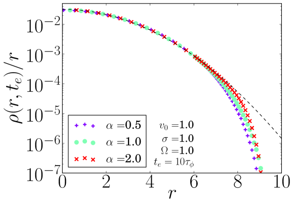
Figure 4: Colored symbols correspond to simulation results according to our full system (1),(2) for the displacement $\rho(r,t_{e})/r$ in polar coordinates divided by $r$, for different values of $\alpha$. Black dashed line according to equation (32) is the diffusion approximation. Parameters as given in the figures and $\tau_{\phi}=1$ for all curves.

Figure 4 shows the displacements’ density for our initial system and the results of our approximation. Symbols correspond to simulation results for the initial system Eqs. (1),(2). The black dashed line shows the the Rayleigh distribution divided by $r$, for $t=10\tau_{\phi}$. For $r\ll v_{0}t$ the approximation works well. The curve starts to deviate at distances larger then the mean squared displacement, which in this case occurs when $r\,\approx\,6$.

Close to the maximal distance $r=v_{0}t$ the approximation breaks down since it neglects the existence of the maximal absolute velocity and therefore the truncation of the displacements’ distribution. As can be seen from the simulation results, the index $\alpha$ of the noise influences weakly the exact form of the decay of $\rho(r,t)$ to zero.

Thus, the coarse grained dynamics of our micro-swimmer with angular component driven by symmetric $\alpha-$stable noise and constant torque can be described by the standard Langevin equations

$$\frac{d\vec{r}}{dt}=\sqrt{2D_{\text{eff}}}\vec{\xi},$$ (33)

where two independent Gaussian noise sources $\vec{\xi}=(\xi_{x},\xi_{y})$ drive the motion, with $\langle\xi_{i}\rangle=0$ and $\langle\xi_{i}(t)\xi_{j}(t^{\prime})\rangle=\delta_{ij}\delta(t-t^{\prime})$, where $i,j=x,y$.

v) In the limit $t\gg\tau_{\phi}$ the trajectories of stochastic microswimmers with constant speed are indistinguishable from the paths created by a Brownian particle as predicted by Eq. (33) with noise possessing $\alpha=2$. The question what kind of noise drives the heading is then addressed to the dependence of the diffusion coefficient on the parameter $\alpha$. Following Eq. (4) and Eq. (3), the diffusion coefficient scales in case of strong noise as

$$D_{\text{eff}}\,\propto\,v_{0}^{2}\,\tau_{\phi}\,=\,\frac{v_{0}^{2+\alpha}}{\sigma^{\alpha}}\,.$$ (34)

The experimentally accessible value is the velocity $v_{0}$ of the microswimmer, rather than the noise intensity $\sigma$ of the torque. Hence, the inspection of the diffusion coefficient’s dependence on the velocity may give hints onto the possible presence of the $\alpha$-stable noise. Furthermore, we emphasize that the diffusion coefficient scales counterintuitively as $D_{\text{eff}}\,\propto 1/\sigma^{\alpha}$ with the noise intensity, parallel to what is known for $\alpha=2$ mikhailov .

vi) The influence of the torque induces an anti-symmetric part in the matrix of the Onsager coefficients connecting the momentum flux with the derivative of the density in Eq. (25). The latter results in a rotation matrix with the rotation angle $\phi_{\Omega}$ which is defined as $\sin(\phi_{\Omega})=\Omega\tau_{\phi}/\sqrt{1+\Omega^{2}\tau_{\phi}^{2}}$. In compact form the connections Eq. (25) read

$$\rho\vec{u}\,=\,-\frac{\tau_{\phi}}{\sqrt{1+\Omega^{2}\tau_{\phi}^{2}}}\frac{v_{0}^{2}}{2}\begin{pmatrix}~{}\cos(\phi_{\Omega})~{}~{}~{}~{}-\sin(\phi_{\Omega})\\ \sin(\phi_{\Omega})~{}~{}~{}~{}\cos(\phi_{\Omega})\end{pmatrix}\,\vec{\nabla}\rho\,.$$ (35)

In conclusion, we considered an active particle moving at a constant speed, with constant torque and random fluctuations in the heading. Such particles exhibit ballistic motion at small time scales $t<\tau_{\phi}$ and diffusive behavior at larger times. We showed that starting from the Fokker Planck equation for the joint probability density of the position and the heading, the orientation as a persistent variable can be eliminated by means of reduced moments for all symmetric $\alpha$-stable noise sources. This leads to the diffusion equation for the corresponding coarse grained dynamics. In consequence, the resulting particle dynamics becomes that of a Brownian particle.

VI Acknowledgments

This work was supported by the Deutsche Forschungsgemeinschaft via IRTG 1740. LSG thanks Ohio University in Athens OH and especially A. B. Neiman for hospitality and support. The authors thank Vander Freitas (Sao Jose dos Campos) for pointing out the behavior of fruit flies. The authors thank Christophe Haynes for fruitful discussions.

Appendix A Adiabatic elimination using the Langevin equation for Gaussian white noise

In the case of Gaussian white noise ($\alpha=2$), it is possible to use the Langevin equations Eq. (1) and Eq. (2) to eliminate the persistent variable. We outline here this approach for the sake of completeness. To be consistent with our previous definition, we require $\langle\xi(t)\xi(t^{\prime})\rangle=2\delta(t-t^{\prime})$.

Taking the time derivative of the velocity components

$$\dot{v}_{x}=\frac{v_{0}(\cos(\phi(t)+{\rm d}\phi)-\cos(\phi(t))}{{\rm d}t}=\frac{v_{0}(\cos(\phi)\cos({\rm d}\phi)-\sin(\phi)\sin({\rm d}\phi)-\cos(\phi))}{{\rm d}t}\,,$$ (36)

(with ${\rm d}t\rightarrow 0$) allows for a compact description. Stratonovich calculus stratonovich will be used later on.

According to Eq. (2) the angular increment reads:

$${\rm d}\phi=\frac{1}{\tau_{\phi}}{\rm d}W_{t}+\Omega{\rm d}t,$$ (37)

with ${\rm d}W_{t}$ being the Wiener process, with the average properties: $\langle{\rm d}W_{t}\rangle=0$, $\langle{\rm d}W_{t}{\rm d}W_{t^{\prime}}\rangle=0$ for $t\neq t^{\prime}$ and $\langle{\rm d}W_{t}{\rm d}W_{t^{\prime}}\rangle=2{\rm d}t$ for $t=t^{\prime}$. The non-averaged squared increment behaves as $({\rm d}W_{t})^{2}\,=\,2{\rm d}t\,+\,\mathcal{O}({\rm d}t^{3/2})$. Taking ${\rm d}\phi$ small, the change in velocity can be rewritten as

$$\dot{v}_{x}\,=\,-\frac{v_{0}(\cos(\phi)\frac{{\rm d}\phi^{2}}{2}+\sin(\phi){\rm d}\,\phi)}{{\rm d}t}\,.$$ (38)

Up to first order of ${\rm d}t$ this equation reduces to

$$\dot{v}_{x}=-\frac{1}{\tau_{\phi}}\left(v_{x}+\Omega\tau_{\phi}v_{y}+\sqrt{v_{0}^{2}\tau_{\phi}}\sin(\phi)\,\xi_{\phi}(t)\right).$$ (39)

In this expression we extracted the relaxation time introduced in Eq. (3) for $\alpha=2$.

Now we can adiabatically eliminate the change in velocity. For times larger than the relaxation time $t\gg\tau_{\phi}$, we reach the limit, corresponding to $\dot{v}_{x}\tau_{\phi}\to 0$. The velocity reads now:

$$v_{x}\,=\,-\Omega\tau_{\phi}v_{y}-\sqrt{v_{0}^{2}\tau_{\phi}}\sin(\phi)\,\xi_{\phi}(t)\,.$$ (40)

The velocity in the $y$ direction can be determined following the same lines:

$$v_{y}\,=\,-\Omega\tau_{\phi}v_{x}-\sqrt{v_{0}^{2}\tau_{\phi}}\cos(\phi)\,\xi_{\phi}(t)\,.$$ (41)

Both velocities depend on each other. Eliminating these dependencies, i.e. substituting one equation into the other one, results in the closed equations

$$v_{x}\,=\,-\frac{1}{1+\left(\Omega\tau_{\phi}\right)^{2}}\,\left(\sin(\phi)\,+\,\Omega\tau_{\phi}\cos(\phi)\right)\,\sqrt{v_{0}^{2}\tau_{\phi}}\xi_{\phi}(t)$$ (42)

and

$$v_{y}\,=\,\frac{1}{1+\left(\Omega\tau_{\phi}\right)^{2}}\,\left(\cos(\phi)\,-\,\Omega\tau_{\phi}\sin(\phi)\right)\,\sqrt{v_{0}^{2}\tau_{\phi}}\xi_{\phi}(t)\,.$$ (43)

We point out that the same noise $\xi_{\phi}(t)$ is acting in both projections of the velocity. Further more, it should be noted that the angle $\phi(t)$ and the noise $\xi_{\phi}(t)$ are statistically independent since the former depends only on the values of $\xi(t^{\prime})$ at previous instants of time.

We now can calculate the velocity correlation function $C_{v,v}(t-t^{\prime})=\langle\vec{v}(t)\cdot\vec{v}(t^{\prime})\rangle$ and obtain

$$C_{v,v}(t-t^{\prime})\,=\,2\frac{v_{0}^{2}\tau_{\phi}}{1+\left(\Omega\tau_{\phi}\right)^{2}}\,\delta(t-t^{\prime})\,.$$ (44)

Thus, the velocity is given by a white noise and inertia has being eliminated.

Nevertheless, the velocity components are still correlated since a single noise source acts in both directions. Only after averaging over the angle $\phi$ with the uniform angular distribution following from equation Eq. (8), for $t\gg\tau_{\phi}$, do the components become uncorrelated;

$$\langle\langle v_{i}(t)v_{j}(t^{\prime})\rangle\rangle_{\phi}\,=\,\frac{v_{0}^{2}\tau_{\phi}}{1+\left(\Omega\tau_{\phi}\right)^{2}}\,\delta(t-t^{\prime})\,\delta_{ij}\,.$$ (45)

In this limit the dynamics can be formulated as defined in Eq. (33), and corresponds to those of a Brownian particle driven by two independent noise sources in both directions. The correlated dynamics Eq. (42) and Eq. (43) still reflects the fact that the noise $\xi_{\phi}(t)$ is acting in a direction perpendicular to the current motion. In case of an additionally acting torque $\Omega$ the two forces undergo an additional shift which is given by the angle $\phi_{\Omega}$ as defined in the last section. Using this and Eq. (42) and Eq. (43) the two components reads

$$\dot{x}\,=\,v_{x}\,=\,-\sqrt{\textbullet 2D_{\rm eff}}\,\sin(\phi(t)+\phi_{\Omega})\,\xi_{\phi}(t)$$

$$\dot{y}\,=\,v_{y}\,=\,\sqrt{\textbullet 2D_{\rm eff}}\,\cos(\phi(t)+\phi_{\Omega})\,\xi_{\phi}(t)\,.$$ (46)

We remember that $\phi(t)$ defines the heading, i.e. the current direction of motion. In Eq. (46) the velocity or the displacement points perpendicular to the direction given by the angle $\phi(t)+\phi_{\Omega}$. In particular, without torque $\Omega=0$, it acts perpendicular to the current motion.

Eq. (46) can be interpreted as an algorithm for the considered coarse grained microswimmer. For time scales $t\gg\tau_{\phi}$ both $\phi(t)$ and $\xi_{\phi}(t)$ are statistically independent. $\phi(t)$ is a white noise homogeneously distributed in $[0,2\pi]$ and $\xi_{\phi}(t)$ is Gaussian white noise. The process $\phi(t)$ after the elimination procedure does not possess any memory and is in the considered case of $\alpha=2$ the increment of the Wiener process. Therefore in the approximation, the microswimmer changes suddenly the direction of motion following a Wiener process shifted by $\phi_{\Omega}$ and increments are added in direction perpendicular to $\phi(t)+\phi_{\Omega}$.

Appendix B Moments of the angular dynamics:

In contrast to the consideration in the main part of this article, we start here with the pdf $\tilde{P}(x,\phi,t|x_{0},\phi_{0},t_{0})$, defined for $\phi\in(-\infty,+\infty)$. Later on, we again omit the explicit statement of the condition.

The connection between the the unwrapped and the wrapped distribution function $P(x,\phi,t)$ can be formulated as follows

$$P(x,\phi,t)\,=\,\sum_{n=-\infty}^{\infty}\,\tilde{P}(x,\phi+2\pi n,t)\,,$$ (47)

where now $\phi\in[0,2\pi)$ and the wrapped pdf is normalized in this interval.

As $\tilde{P}(x,\phi,t)$ is a probability density, it fulfills

$$\tilde{P}(x,\phi,t)\geq 0,$$ (48)

and

$$\int_{-\infty}^{\infty}\,{\rm d}\phi\,\tilde{P}(x,\phi,t)\,<\,\infty;\,\,\,\forall x,t.$$ (49)

The expectation values $\langle\cos^{n}(\phi)\rangle,~{}~{}n\,\geq\,1$ will exist as well since the following holds

$$\left|\int_{-\infty}^{\infty}\,{\rm d}\phi\,\cos^{n}(\phi)\,\tilde{P}(x,\phi,t)\right|\,\leq\,\int_{-\infty}^{\infty}\,{\rm d}\phi\,\tilde{P}(x,\phi,t)\,,$$ (50)

as $|\cos^{n}(\phi)|\leq 1$ is bounded. Similarly, we proceed with $\langle\sin(\phi)^{n}\rangle$.

During the derivation of the transport equations we have used the following identities and properties of the pdf

$$\int_{-\infty}^{\infty}\,{\rm d}\phi\,\cos(\phi)\,\frac{\partial^{\alpha}}{\partial|\phi|^{\alpha}}\,\tilde{P}(x,\phi,t)\,=\,\frac{1}{2\pi}\,\int_{-\infty}^{\infty}\int_{-\infty}^{\infty}\,{\rm d}k{\rm d}\phi\,\cos(\phi)\,\frac{\partial^{\alpha}}{\partial|\phi|^{\alpha}}e^{-ik\phi}\,\tilde{P}(x,k,t)$$

$$=\,-\,\frac{1}{2\pi}\int_{-\infty}^{\infty}\int_{-\infty}^{\infty}\,{\rm d}k{\rm d}\phi|\,k|^{\alpha}\cos(\phi)e^{-ik\phi}\,\tilde{P}(x,k,t)\,=\,-\,\frac{1}{2}\left(\tilde{P}(x,1,t)\,+\,\tilde{P}(x,-1,t)\right)\,.$$

where $\tilde{P}(x,k,t)$ is the Fourier transform of $\tilde{P}(x,\phi,t)$ in its angular variable. Otherwise, it holds that

$$\int_{-\infty}^{\infty}{\rm d}\phi\,\cos(\phi)\,\tilde{P}(x,\phi,t) = \frac{1}{2\pi}\,\int_{-\infty}^{\infty}\int_{-\infty}^{\infty}\,{\rm d}k{\rm d}\phi\,\cos(\phi)e^{-ik\phi}\,\tilde{P}(x,k,t)$$

$$= \frac{1}{2}\,\left(\tilde{P}(x,1,t)\,+\,\tilde{P}(x,-1,t)\right)\,.$$

It follows that

$$\int_{-\infty}^{\infty}\,{\rm d}\phi\,\cos(\phi)\,\frac{\partial^{\alpha}}{\partial|\phi|^{\alpha}}\,\tilde{P}(x,\phi,t)\,=\,-\,\int_{-\infty}^{\infty}{\rm d}\phi\,\cos(\phi)\,\tilde{P}(x,\phi,t)\,.$$ (51)

Analogously, we derive the identities:

$$\int_{-\infty}^{\infty}{\rm d}\phi\,\sin(\phi)\frac{\partial^{\alpha}}{\partial|\phi|^{\alpha}}\tilde{P}(x,\phi,t)\,=\,-\int{\rm d}\phi\,\sin(\phi)\tilde{P}(x,\phi,t)\,.$$ (52)

$$\int_{-\infty}^{\infty}{\rm d}\phi\,\cos^{2}(\phi)\,\frac{\partial^{\alpha}}{\partial|\phi|^{\alpha}}\,\tilde{P}(x,\phi,t)\,=\,-2^{\alpha}\,\int_{-\infty}^{\infty}{\rm d}\phi\,\left(\cos^{2}(\phi)\,-\,\frac{1}{2}\,\right)\,\tilde{P}(x,\phi,t)\,,$$

$$\int_{-\infty}^{\infty}{\rm d}\phi\,\sin^{2}(\phi)\,\frac{\partial^{\alpha}}{\partial\,|\phi|^{\alpha}}\,\tilde{P}(x,\phi,t)\,=\,2^{\alpha}\int_{-\infty}^{\infty}{\rm d}\phi\,\left(\cos^{2}(\phi)\,-\,\frac{1}{2}\right)\,\tilde{P}(x,\phi,t)\,,$$

$$\int_{-\infty}^{\infty}{\rm d}\phi\,\cos(\phi)\sin(\phi)\,\frac{\partial^{\alpha}}{\partial|\phi|^{\alpha}}\,\tilde{P}(x,\phi,t)\,=\,-2^{\alpha}\,\int_{-\infty}^{\infty}{\rm d}\phi\,\cos(\phi)\sin(\phi)\,\tilde{P}(x,\phi,t)\,.$$

The derived relations express properties of the generating function of the $\alpha$-stable noise. They hold as well for the wrapped distribution with different integration limits due to the linear connection (47) between both presentations.

References

- (1) P. Romanczuk, L. Schimansky-Geier, Phys. Rev. Lett. 106, 230601 (2011).
- (2) R. Großmann, F. Peruani, M. Bär New J. Phys. 18, 043009 (2016).
- (3) M. Mijalkov, G. Volpe, Soft Matter, 9, 6376 (2013).
- (4) G. Volpe, S. Gigan, G. Volpe, Am. J. Phys. 82, 659 (2014).
- (5) A. Geiseler, P. Hänggi, F. Marchesoni, C. Mulhern, S. Savel’ev Phys. Rev. E 94, 012613 (2016).
- (6) A. Geiseler, P. Hänggi, P. Schmid, G. Eur. Phys. J. 89, 175 (2016).
- (7) A. Patch, D. Yllanes, M.C. Marchetti, Phys. Rev. E 95, 012601 (2017).
- (8) D. Debnath, P.K. Ghosh, Y. Li, F. Marchesoni, B. Li, Soft Matter 12, (2016).
- (9) B. ten Hagen, S. van Teeffelen, H. Löwen, J. Phys: Condensed Matter 23 194119 (2011).
- (10) S. Babel, B. ten Hagen, H. Löwen, J. Stat. Mech. 2014 P02011 (2014).
- (11) W.R. DiLuzio, L. Turner, M. Mayer, P. Garstecki, Nature 435, 1271 (2005).
- (12) J. Hill, O. Kalkanci, J.L. Mc. Murry, H. Koser, Phys. Rev. Lett. 98, 068101 (2007).
- (13) D.M. Woolley, Reproduction (Bristol U.K.) 126, 259 (2003)
- (14) I.H. Riedel, K. Kruse, J. Howard, Science 309, 300 (2005).
- (15) S. van Teeffelen, H. Löwen, Phys. Rev. E 78(2), 020101 (2008).
- (16) B.M. Friedrich, F. Jülicher, New J. Phys. 10, 123025 (2008).
- (17) P. Dhar, T.M. Fischer, Y. Wang, T.E. Mallouk, W.F. Paxton, A. Sen, Nano Lett. 6, 66 (2006).
- (18) A. Kudrolli, G. Lumay, D. Volfson, L.S. Tsimring, Phys. Rev. Lett. 100, 058001 (2008).
- (19) F. Kümmel, B. ten Hagen, R. Wittkowski, I. Buttinoni, R. Eichorn, G. Volpe, H. Löwen, and C. Bechinger, Phys. Rev. Lett. 110,198302 (2013).
- (20) W. Blum, W. Riegler, L. Rolandi, Particle Detection with Drift Chambers, 2nd ed. (Springer, Berlin, Heidelberg, 2008).
- (21) C. Weber, I.M. Sokolov, L. Schimansky-Geier, Phys. Rev. E 85, 052101 (2012).
- (22) C. Weber, P.K. Radtke, L. Schimansky-Geier, P. Hänggi Phys.Rev.E 84, 011132 (2011).
- (23) J. Noetel, I.M. Sokolov, L. Schimansky-Geier, J. Phys. A: Math. Theor.50 034003 (2017).
- (24) P. Langevin, C. R. Acad. Sci (Paris) 146, 530 (1908).
- (25) R. Becker,Theorie der Wärme (Springer, Berlin, 1955);Theory of Heat(Springer, Heidelberg et al., 1965), chapter VI B.
- (26) L. H’walisz, P. Jung, P. Hänggi, P. Talkner, L. Schimansky-Geier, Z.Phys.B 77, 471 (1989).
- (27) S. Milster, J. Noetel, I.M. Sokolov, L. Schimansky-Geier, Eur. Phys. J. Special Topics 226, 2039 (2017).
- (28) H. A. Kramers, Physica 7, 284 (1940).
- (29) H. Haken, Synergetics-an Introduction, 2nd ed. (Springer, Berlin, 1978), Chap. 7.
- (30) C. W. Gardiner, Handbook of Stochastic Methods(Springer, 1983).
- (31) C. W. Gardiner, Phys. Rev. A 29, 2814(1984).
- (32) P. Jung and P. Hänggi, Phys. Rev. A 35, 4464 (1987).
- (33) L. Schimansky-Geier and P. Talkner, in Stochastic Dynamics of Reacting Macromolecules, ed. by W. Ebeling, L. Schimansky-Geier, and Yu. M. Romanovsky, World Sientific, Singapore (2002).
- (34) J. M. Sancho, Phys. Rev. E 84, 062102 (2011).
- (35) W. Feller, An Introduction to Probability Theory and It’s Applications (John Wiley & Sons, New York, 1968,), pp. 169ff.
- (36) J.-F. Rupprecht, O. Benichou, and R, Voituriez, Phys. Rev. E 94, 012117 (2014).
- (37) F. Thiel, L. Schimansky-Geier, and I.M. Sokolov, Phys. Rev. E 86, 021117 (2012).
- (38) I. S. Kim and M. H. Dickinson, Current Biology 27, 2227 (2018).
- (39) B. el Jundi, Current Biologyy 27, R746 (2017).
- (40) P.D. Ditlevsen, Phys. Rev.E 60, 172 (1999)
- (41) D. Schertzer, M. Larchevêque, J. Duan, V.V. Yanowsky, and S. Lovejoy, J. Math. Phys. 42, 200 (2001).
- (42) A. Mikhailov, D. Meinköhn, in Stochastic Dynamics, edited by L. Schimansky-Geier, T. Pöschel, Springer (1997).
- (43) R.L. Stratonovich, SIAM J. Control 4, 362 (1966); Topics in the Theory of Random Noise 1 (Gordon and Breach, New York 1963), pp. 89ff.