GAMA/G10-COSMOS/3D-HST: The $0<z<5$ cosmic star-formation history, stellar- and dust-mass densities

Abstract

We use the energy-balance code MAGPHYS to determine stellar and dust masses, and dust corrected star-formation rates for over 200,000 GAMA galaxies, 170,000 G10-COSMOS galaxies and 200,000 3D-HST galaxies. Our values agree well with previously reported measurements and constitute a representative and homogeneous dataset spanning a broad range in stellar mass ($10^{8}$—$10^{12}$M_⊙), dust mass ($10^{6}$—$10^{9}$M_⊙), and star-formation rates ($0.01$—$100$M_⊙yr^-1), and over a broad redshift range ($0.0<z<5.0$). We combine these data to measure the cosmic star-formation history (CSFH), the stellar-mass density (SMD), and the dust-mass density (DMD) over a 12 Gyr timeline. The data mostly agree with previous estimates, where they exist, and provide a quasi-homogeneous dataset using consistent mass and star-formation estimators with consistent underlying assumptions over the full time range. As a consequence our formal errors are significantly reduced when compared to the historic literature. Integrating our cosmic star-formation history we precisely reproduce the stellar-mass density with an ISM replenishment factor of $0.50\pm 0.07$, consistent with our choice of Chabrier IMF plus some modest amount of stripped stellar mass. Exploring the cosmic dust density evolution, we find a gradual increase in dust density with lookback time. We build a simple phenomenological model from the CSFH to account for the dust mass evolution, and infer two key conclusions: (1) For every unit of stellar mass which is formed $0.0065$—$0.004$ units of dust mass is also formed; (2) Over the history of the Universe approximately 90 to 95 per cent of all dust formed has been destroyed and/or ejected.

1 Introduction

Since recombination the baryonic mass in the Universe has transformed from a smooth atomic distribution of neutral gas, to ionised gas (i.e., reionisation), and thereafter into a number of distinct forms. Most notably residual ionised gas, neutral gas (HI), molecular gas, stars, dust, and super-massive black holes (SMBHs). The redistribution of the primordial re-ionised plasma over time is of pertinent scientific interest. Most of the action, in terms of transformational processes, occur in the context of galaxy formation and evolution. This is moderated by the dominating gravitational field of the underlying dark matter halo, galaxy-galaxy interactions, and gas accretion, all of which drive a multitude of astrophysical processes which give rise to changes in the cosmic gas, stellar, dust, and SMBH densities over time.

The current baryon inventory (see Shull, Smith & Daniforth 2012), suggests that today’s baryonic mass can be roughly broken down into the following forms:

UNBOUND:

— hot ionised plasma (28 per cent; Fukugita, Hogan & Peebles 1998; Shull, Smith & Danforth 2012)

— the Warm Hot Intergalactic Medium (29 per cent; Shull, Smith & Danforth 2012)

BOUND TO CLUSTER AND GROUP HALOSs:

— the intra-cluster light (4 per cent; Shull, Smith & Danforth 2012)

— the intra-group light ($<1$ per cent; Driver et al. 2016)

BOUND TO GALAXY HALOS:

— stars (6 per cent Baldry, Glazebrook & Driver 2008, 2012; Peng et al. 2010; Moffett et al. 2016; Wright et al. 2017a)

— neutral gas (2 per cent; Zwaan et al. 2005; Martin et al. 2010; Delhaize et al. 2013; Martindale et al. 2017)

— circum-galactic medium (5 per cent Shull, Smith & Danforth 2012; Stocke et al. 2013)

— molecular gas (0.2 per cent; Keres et al., 2003; Walter et al. 2014)

— dust (0.1 per cent Vlahakis, Dunne & Eales 2005; Driver et al. 2007; Dunne et al. 2011; Clemens et al. 2013; Beeston et al. 2017)

— SMBHs (0.01 per cent Shankar et al. 2004; Graham et al. 2007 ; Vika et al. 2009 ; Mutlu Pakdil, Seigar & Davis 2016)

UNACCOUNTED FOR:

— missing baryons (25 per cent; see also Shull, Smith & Danforth 2012)

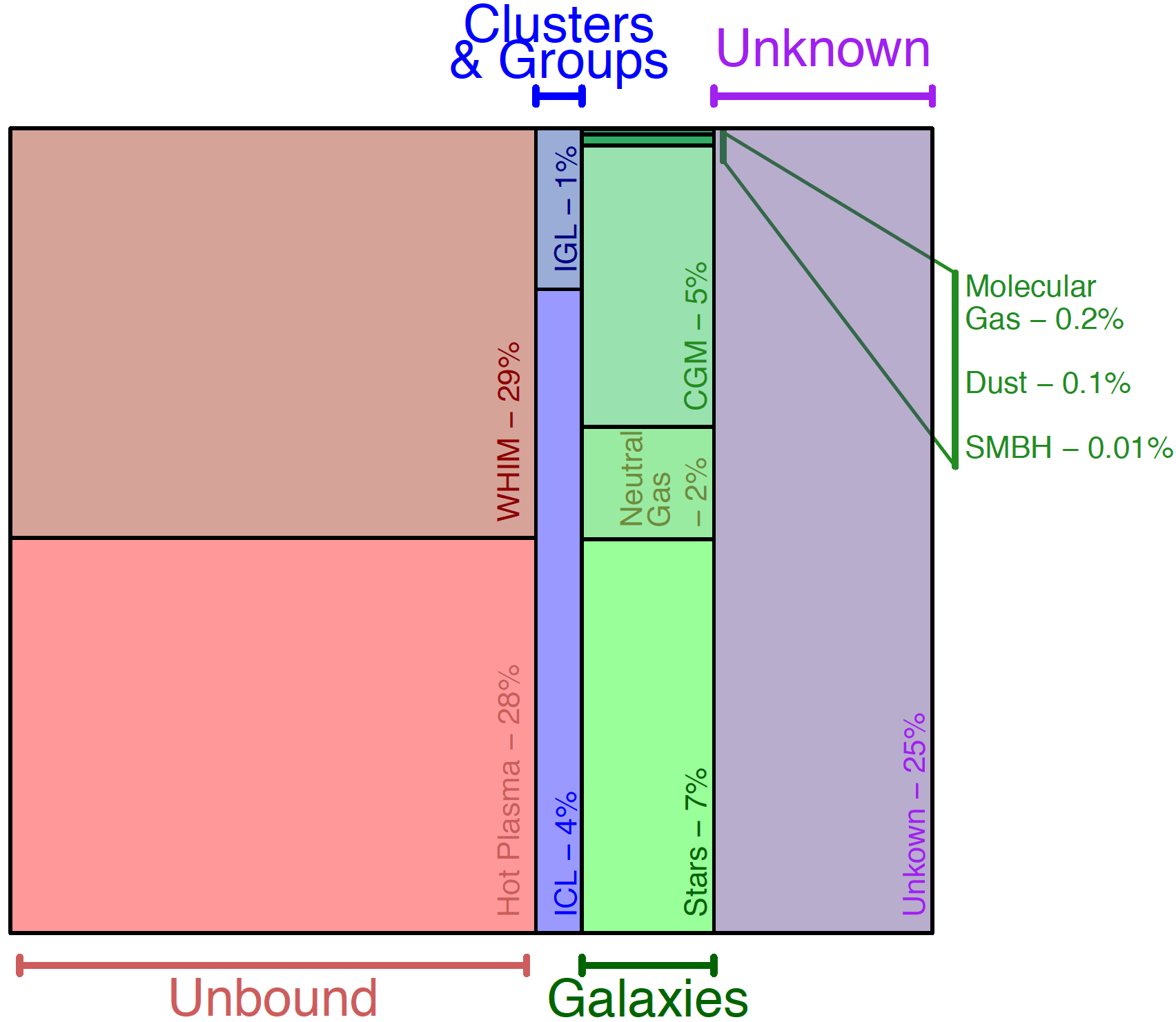
Figure 1: The baryon budget divided into bound and unbound repositories as well as gas, dust, and stellar sub-components. Data mostly derived from Shull, Smith & Danforth (2012) with updates as described in the text.

These components (see Fig. 1) sum to form the baryon budget (Fukugita, Hogan & Peebles 1998), which can be compared to the baryon density implied from cosmological experiments, e.g., Wilkinson Microwave Anisotropy Probe (WMAP; Hinshaw et al. 2013), Planck (Ade et al. 2016), and various constraints on Big Bang Nucleosynthesis (BBN; Cyburt et al. 2016). At the moment some tension exists between cosmological versus local inventories (Shull, Smith & Danforth 2012). However significant leeway (i.e., $\pm 50$ per cent) is available in almost all of the mass repositories listed above. The dominant ionised component, in particular, is extremely hard to robustly constrain and can be crudely divided into: unbound free-floating and very hot ionised gas ($T\sim 10^{6-8}$ K); the loosely bound Warm Hot Inter-galactic Medium (WHIM; $T\sim 10^{4-6}$K); the bound hot intra-cluster/group light (ICL/IGL; $T\sim 10^{6-7}$K); and the bound circum-galactic plasma ($T\sim 10^{6}$K).Cooler components also cannot be ruled out (i.e., $10^{2}-10^{4}$K). These components, illustrated in Fig. 1, and their associated errors, are discussed in Shull, Smith & Danforth (2012) who first articulated concerns over the missing $\sim 30$% of baryons as compared to WMAP and BBN analyses. A more statistical approach based on the kinematic Sunyaev-Zeldovich effect in the Planck Cosmic Microwave Background dataset (Hernández-Monteagudo et al. 2015) does suggest that the bulk of the baryons closely follow the dark-matter distribution and, based on opacity arguments, argue for an additional ionised component beyond that seen via traditional X-ray absorption lines. Recently an additional hot-WHIM component has been reported by Bonamente et al. (2016), as well as an overdensity of the WHIM along the cosmic web (Eckert et al. 2015). However, conversely, Danforth et al. (2015) revisited the estimates of Shull et al., and reported a lower value for the directly detected gas. Essentially sufficient uncertainty exists which suggests that the bulk of the missing baryons is most likely in an ionised component, that closely follows the underlying dark-matter distribution.

Comparable uncertainty at a similar $\pm 50$ per cent level potentially exists in the more minor components, i.e., the neutral gas, molecular gas, stellar, dust and SMBH components associated with galaxies (with all other repositories considered insignificant compared to these, e.g., planets and planetesimals). To some extent these are linked, i.e., if one identifies more stellar mass in the form of an additional galaxy population the other components would likely increase too (i.e., the associated CGM, HI etc). Also of interest is the change in these bound components with time as gas is converted into stars, metals, and dust.

Measurements of the galaxy population suggests that over the past few Gyrs the stellar mass and HI cosmic co-moving density has plateaued (see Wilkins, Trentham & Hopkins. 2008; Delhaize et al. 2013), while the molecular mass density has declined with time (Walter et al. 2014; Decarli et al. 2016), and the cosmic dust density declined rapidly over late epochs (Dunne et al. 2011). The latter molecular gas and dust density declines are arguably driven by the decline in the cosmic star-formation history (Lilly et al. 1996; Hopkins & Beacom 2006; Madau & Dickinson 2014). One of the key goals of the Galaxy And Mass Assembly (GAMA) project (Driver et al. 2009; 2011) is to quantify the baryon components contained within galaxies, and to empirically recover their recent evolution. In this study we focus in particular on the cosmic star-formation history (CSFH), the stellar mass density (SMD), and dust mass density (DMD).

Central to a robust estimate of the bound mass components, is the determination of consistent stellar and dust mass estimates over a sufficiently large area to overcome cosmic variance (Driver & Robotham 2010), and over a sufficiently large redshift baseline to probe time evolution. This inevitably requires extensive observations on multiple ground and space-based facilities. Over the past 7 years we have assembled an extensive database of panchromatic photometry (Driver et al. 2016) extending from the UV to the far-IR over a combined 230sq deg region of sky and which builds upon a deep Australian/European spectroscopic campaign of 300,000 galaxies (with $r<19.8$ mag and $z\leq 0.5$; Driver et al. 2011; Liske et al. 2015). This dataset has been constructed from a number of independent survey programs including GALEX (Martin et al. 2005), SDSS (York et al. 2000), VIKING (Sutherland et al. 2015), WISE (Wright et al. 2010), and Herschel-ATLAS (Eales et al. 2010; Valiante et al. 2016; Bourne et al. 2017). In parallel, a similar US/European/Japanese effort has obtained extremely deep panchromatic imaging over the Hubble Space Telescope (HST) Cosmology Evolution Survey (COSMOS) region (Scoville et al. 2007a,b), while a USA-led group have built extensive multiwavelength and GRISM observations of notable HST deep fields as part of the 3D-HST study (see van Dokkum et al. 2013; Brammer et al. 2012 and Momcheva et al. 2016).

We have recently completed the task of assimilating and homogenising the first two of these datasets (GAMA and G10-COSMOS) into the GAMA database, using an identical software analysis pathway for object detection (SExtractor; Bertin et al. 2017), redshift estimation (Baldry et al. 2014; Liske et al. 2015; Davies et al. 2015), and panchromatic flux measurement (Wright et al. 2016; Andrews et al. 2017a). For the 3D-HST dataset we use the online database of panchromatic photometry and redshifts as provided by the 3D-HST team (see Momcheva et al. 2016 and references therein).

A crucial step in homogenising these three surveys, is to obtain consistent star-formation rate, stellar mass, and dust mass estimates. For this purpose we look to the MAGPHYS energy balance code provided by da Cunha, Charlot & Elbaz (2008). MAGPHYS takes as input a redshift and a series of flux measurements (and errors) spanning the UV to far-IR wavelength range. It then compares the observed flux measurements to an extensive stellar spectral and dust emission library to obtain an optimal spectral energy distribution (SED); and where the energy attenuated by dust in the UV/optical/near-IR, balances with the energy radiated in the far-IR. Parameters constrained by this process include the unattenuated star-formation rate, stellar mass, and total dust mass along with information on the opacity, temperature of the ISM and birth clouds, age, metallicity and the unattenuated and attenuated best fit spectral energy distributions.

In Section 2 we provide summary information on our three adopted datasets: GAMA, G10-COSMOS and 3D-HST. In Section 3 we describe the process of MAGPHYS analysis of almost 600,000 galaxy SEDs using the Australian Research Council Pawsey Supercomputing Facility. We explore and validate the datasets in the latter part of Section 3 before finally presenting the cosmic star-formation history and the evolution of the stellar and dust mass densities since $z=5$ in Section 4. In Section 5 we discuss the implications of our results compared to numerical simulations, attempt to build a phenomenological model to explain the stellar mass and dust density from the CSFH and finish by placing our measurements into the context of the evolution of the bound baryon budget.

This empirical paper therefore forms the basis for a series of further papers which explore: the very faint-end of the stellar mass function and the prospect of missing diffuse low-surface brightness galaxies (Wright et al. 2017a); the HI and baryonic mass function (Wright et al. 2017b); the faint-end of the low-redshift dust mass function (Beeston et al. 2017); the evolution of the cosmic spectral energy distribution (Andrews et al. 2017b); and detailed modelling of the evolution of the cosmic spectral energy distribution with time (Andrews et al. 2017c).

In general these studies extend our existing knowledge by providing consistent homogeneous measurements over very large volumes, across a very broad range of stellar mass and lookback times, thereby minimising the impact of cosmic (sample) variance.

Throughout we use a concordance cosmological model of $\Omega_{M}=0.3$, $\Omega_{\Lambda}=0.7$ and $H_{0}=70h_{\rm 70}$ km/s/Mpc and work with a time-invariant Chabrier (2003) IMF.

2 Data

We bring together three complementary datasets: GAMA (Driver et al. 2011; Liske et al. 2015), G10-COSMOS (Davies et al. 2015; Andrews et al. 2017a) and 3D-HST (Momcheva et al. 2016). All three studies contain extensive panchromatic photometry extending from the ultra-violet to mid-infrared wavelengths allowing for robust stellar mass estimates. The GAMA and G10-COSMOS data also contain far-IR measurements or constraints from the Herschel Space Observatory’s SPIRE and PACS instruments (Herschel) by the Herschel-ATLAS (Eales et al. 2010), and HerMES (Oliver et al. 2012) teams respectively. This allows for measurement of dust masses and dust-corrected star formation rates. Collectively all three datasets extend from nearby ($z\leq 0.5$; GAMA), to the intermediate ($z<1.75$; G10-COSMOS), and high-z Universe ($z<5.0$; 3D-HST). Each dataset contains approximately 200k galaxies and collectively sample a broad range in stellar mass, morphological types and lookback time.

In this section we first introduce each of the contributing datasets.

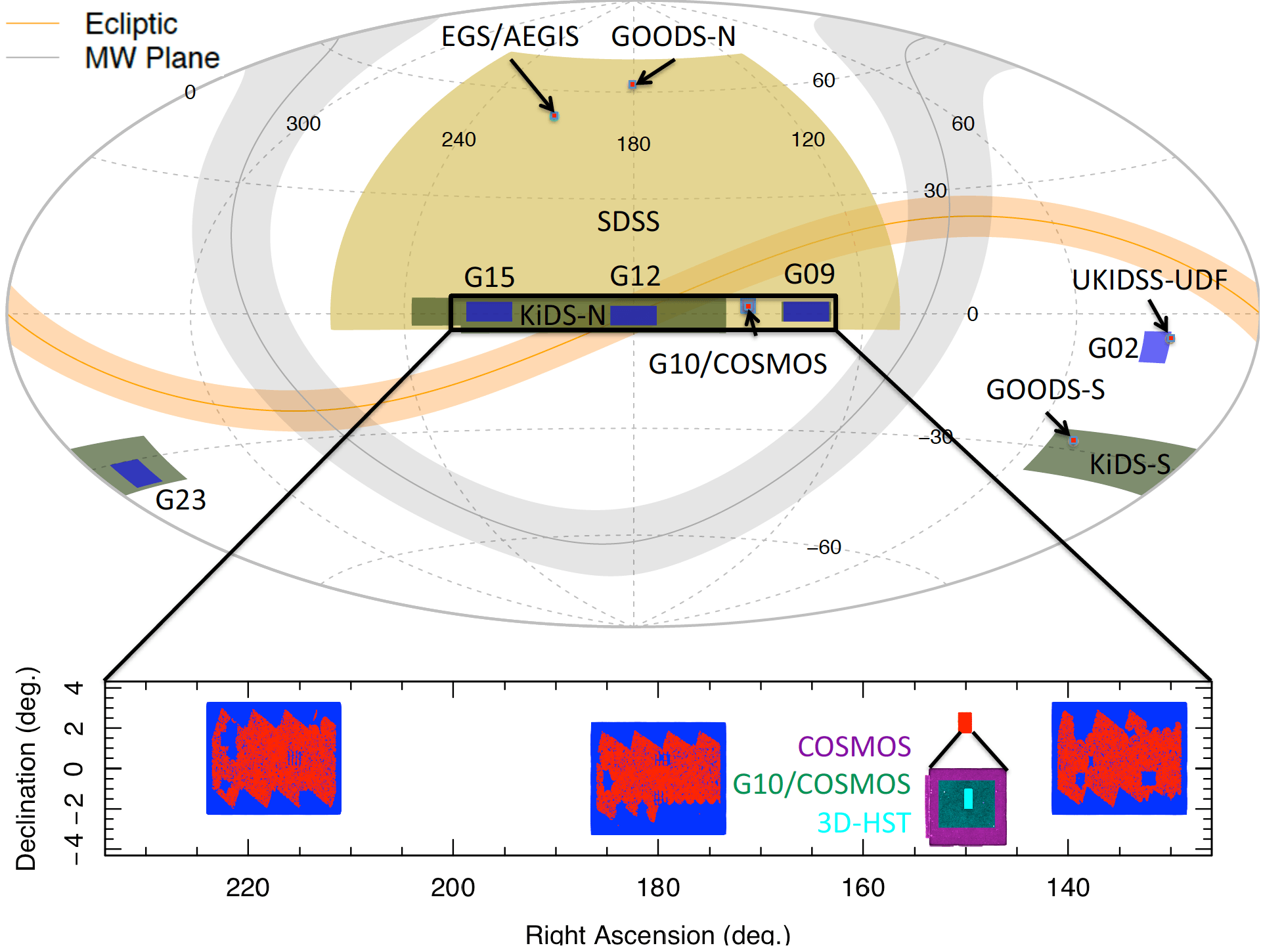
Figure 2: The GAMA, G10-COSMOS and 3D-HST (GOODS-N & -S, UKIDSS-UDS, EGS/AGEIS, COSMOS) survey regions shown on an Aitoff projection of the sky (as indicated). The lower zoom panel highlights the equatorial GAMA regions where blue denotes the full survey regions, and red the distribution of galaxies with complete panchromatic coverage. Also shown in the lower zoom is the various definitions of the COSMOS region, where COSMOS (purple) denotes $\sim 2$ square degree region covered by HST, G10-COSMOS the central square degree with consistent spectroscopic coverage (emerald), and 3D-HST the sub-region with HST GRISM (G141) coverage (cyan). The Aitoff projection is generated via AstroMap: http://astromap.icrar.org/

2.1 Galaxy And Mass Assembly (GAMA)

The Galaxy And Mass Assembly (GAMA) Survey (Driver et al. 2009; 2011) consists primarily of a dedicated spectroscopic campaign to $r<19.8$mag (Driver et al. 2011; Hopkins et al. 2013; Liske et al 2015). It builds upon the two-degree field galaxy redshift survey (2dFGRS; Colless et al. 2001) and the Sloan Digital Sky Survey (SDSS; York et al. 2000). With the latter providing the basis of the GAMA input catalogue for the three equatorial fields using colour and size selection criteria (see Baldry et al. 2010 for details). GAMA overall covers five distinct survey regions (see Fig. 2), including the three equatorial fields at $9^{h}$ (G09), $12^{h}$ (G12) and $14.5^{h}$ (G15). Each of the equatorial survey fields (see Fig. 2, zoom panel) covers a region of $5\times 12$ sq degrees and, to the spectroscopic survey limits, contains approximately 70,000 galaxies within each region. Redshifts have been obtained for $>98$ per cent (see Liske et al. 2015 for the final spectroscopic survey report), with the majority measured by the GAMA team using the AAOmega facility at the Anglo Australian Telescope. In addition to the spectroscopic component, GAMA contains imaging observations from a broad range of ground and space based facilities including: UV (GALEX), optical (SDSS, VST), near-IR (UKIRT, VISTA), mid-IR (WISE), and far-IR (Herschel) imaging. These data have been aggregated and made publicly available through the GAMA Panchromatic Data Release (Driver et al. 2016; see http://gama-psi.icrar.org). Photometric flux measurements in 21 bandpasses (FUV, NUV, $ugriz$, $ZYJHK$, W1234, PACS100/160, SPIRE 250/350/500) have been completed using in-house software (LAMBDAR; Wright et al. 2016). LAMBDAR uses the elliptical apertures obtained via SExtractor and convolves them with the appropriate facility PSF, and manages flux-sharing for blended objects including a contamination target list if provided (e.g., stars in the UV to mid-IR bands and high-z systems in the far-IR bands). For more details on LAMBDAR and access to the photometric catalogue and source code see http://gama-psi.icrar.org/LAMBDAR.php and Wright et al. (2016).

Here we use LAMBDARCatv01 which contains 200,246 objects and extract those with redshifts with quality $nQ\geq 3$ using a name match with TilingCatv43. We remove systems with $z<0.001$, replace measured negative fluxes with zeros (i.e., where MAGPHYS will ignore the flux and use the flux error as an upper limit), and replace fluxes where there is no imaging coverage in that band, with a flux value of $-999$ (i.e., ignored by MAGPHYS). The catalogue is then parsed to the MAGPHYS input format which consists of: ID, redshift, $21\times$[flux, flux-error] (in Jy). Fig. 2 shows the on-sky area, with the GAMA regions shown in blue and the area with complete wavelength coverage in all 21 bands shown in red. Restricting our dataset to this latter area reduces the galaxies with complete SED coverage and valid redshifts from 197,494 to 128,568 and our effective survey area from 180.0 sq deg to 117.2 sq deg. Within this region our final sample is 98 per cent spectroscopically complete to $r<19.8$ mag, with no obvious surface brightness or colour bias (see Liske et al. 2015).

2.2 G10-COSMOS

G10-COSMOS (Davies et al. 2015; Andrews et al. 2017a) is a 1 sq deg sub-region of the HST COSMOS survey (Scoville et al. 2007a,b). It enjoys contiguous coverage from ultra-violet to far-IR wavelengths (Andrews et al. 2017a), including: UV (GALEX), optical (CFHT, Subaru, HST), near-IR (VISTA), mid-IR (Spitzer), and far-IR (Herschel) imaging. These deep data have been obtained from a variety of public websites, and processed in a similar manner to the GAMA data using LAMBDAR (Andrews et al. 2017a). For G10-COSMOS we adopt an $i<25$ mag defined catalogue based on a Source Extractor analysis of the $i$-band Subaru observations (Capak et al. 2007; Taniguchi et al. 2007). This has been followed by extensive efforts to refine the aperture definitions and reject spurious detections (see Andrews et al. 2017a for details). For redshift information we use the updated Davies et al. (2015) catalogue. This includes our independent redshift extraction of the zCOSMOS-Bright sample, combined with spectroscopic redshifts from PRIMUS, VVDS, SDSS (Cool et al. 2013; Le Fevre et al. 2013; Ahn et al. 2014), and photometric redshift estimates from COSMOS2015 (Laigle et al. 2016). The Andrews et al. photometric and updated Davies et al. spectroscopic catalogues are publicly available from http://gama-psi.icrar.org/G10/dataRelease.php

To generate our MAGPHYS input file we adopt G10CosmosLAMBDARCatv06 and extract all objects classified as galaxies and produce an input catalogue with : ID, redshift, $22\times$[flux, fluxerr] containing 142,260 objects (with $z<1.75$). Explicitly the G10-COSMOS dataset has the following filters: FUV,NUV,ugrizYJHK,IRAC1234,MIPS24/70,PACS100/160, SPIRE250/350/500. Note that we do not include the $B$ and $V$ bands because their zeropoints remain somewhat uncertain, and their inclusion would also have the potential to over-resolve the SED fits, particularly given that the majority of these data have photometric rather than spectroscopic redshifts. Because the data arise from multiple facilities, where zero-point errors cannot be entirely ruled out, we implement an error-floor where we set the flux error in each band for each galaxy to be the largest of either the quoted error, or 10 per cent of the flux. Fig. 2 shows the on-sky area with the G10-COSMOS region indicated in both the main panel and the blow-up region.

The G10/COSMO sample is therefore 100 per cent redshift complete to the specified flux limit, with a combination of both spectroscopic and photometric redshifts. For the photometric redshifts the accuracy has been shown to be $\pm 0.0007$ with a catastrophic redshift failure rate of below 0.5 per cent. (see Laigle et al. 2015).

2.3 3D-HST

To extend our stellar mass coverage to the very distant Universe we also include the 3D-HST dataset (Momcheva et al. 2016; Brammar et al. 2012). This was downloaded from the 3D-HST website (version 4.1.5): http://3dhst.research.yale.edu and constitutes a sample of 207,967 galaxies, stars and AGN from five notable deep HST studies. The 3D-HST fields are themselves subregions of the AEGIS, COSMOS, GOODS-S, GOODS-N, and UKIDSS-UDS HST CANDELS fields, for which there is GRISM coverage (WFC3/G141 and/or WFC3/G800L), providing coarse photometric or spectroscopic redshifts over a total of 0.274 sq arcmins (of which 0.174 sq deg is covered by the GRISM data, see Momcheva et al. 2016). Overall the sample has been shown to have a redshift accuracy of $\Delta z/(1+z)=\pm 0.003$, with some expectation that this accuracy will decrease somewhat below $z=0.7$ and towards fainter magnitudes where the bulk of the redshift estimates are purely photometric (see Momcheva et al. 2016 their figures 13 and 14 in particular). In total the 3D-HST catalogue contains 204,294 galaxies and AGN with either a spectroscopic (3839), GRISM (15518), or photometric (185843) redshift estimate. In addition the 3D-HST catalogues also include stellar mass estimates based on SED fitting under the assumption of a Kroupa (2001) IMF (see Skelton et al. 2014). Unfortunately far-IR photometry and hence dust mass estimates do not currently exist for 3D-HST but are in progress as part of the Herschel Extra-galactic Legacy Project (HELP; Hurley et al. 2016). Star-formation rates are estimated via the FAST code of Kriek et al. (2009) as described in Whitaker et al. (2014). These are based on a Chabrier IMF and include consideration of both the UV and mid-IR flux (24 $\mu$m). To be fully consistent with the GAMA and G10-COSMOS datasets we download the panchromatic photometry provided by the 3D-HST team for each field, reformatted and once again apply MAGPHYS to re-determine stellar masses and star-formation rates in a manner consistent with our GAMA and G10-COSMOS derived values.

Fig. 2 shows the location of the five 3D-HST fields on the sky (see also Table. 1 of Momcheva et al. 2016 and their figures 1 and 2). Note that the 3D-HST data is of variable depth with some sub-regions deeper than others. To explore the impact of this “ragged edge” we compare the 3D-HST galaxy number-counts to literature values assembled by Driver et al. (2016) in the F160W band. Fig. 3 shows this comparison which agree well with the 3D-HST data deviating only at very faint magnitudes. The upper panel shows the deviation as a percentage. We see that 3D-HST appears to be 90 percent complete at F160W=25.0 mag (in line with the conclusions of Skelton et al. 2014 and Bourne et al. 2016), reducing to 85 per cent completeness at F160W=26.0 mag. Here we do not adopt a specific flux limit, but note that our sample is effectively limited to $F160W\approx 26.0$ mag.

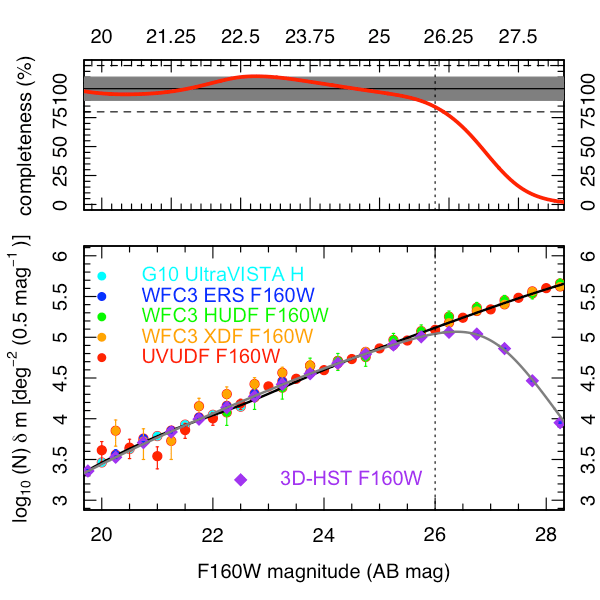
Figure 3: (main panel) Literature galaxy number-counts from HST in the F160W band (Driver e tal. 2016) compared to those from the 3D-HST dataset. (top panel) the deviation as a percentage between a spline fit to the literature values and the 3D-HST data. We adopt a flux limit of F160W=26.0mag which equates to an 20 per cent incompleteness level (i.e., comparable to cosmic variance uncertainties).

2.4 AGN contamination

AGN contamination of all three samples could result in erroneously high stellar masses, and star-formation rates for a small number of interlopers. The impact on dust masses is less obvious as the dust is fairly impervious to the heating mechanism. For our star-formation and stellar mass census it is therefore important to clean our catalogues of AGN. First we remove significant outliers in stellar mass, i.e., all systems with masses greater than $10^{12}$ M_⊙, this equates to 32, 2, and 66 objects in GAMA, G10-COSMOS and 3D-HST respectively. For each catalogue we then adopt the following strategy to remove AGN contaminants:

GAMA: No AGN removal is attempted, beyond the mass cut mentioned above, as the density at $z\leq 0.5$ is extremely low and any AGN component likely to be sub-dominant.

G10-COSMOS: We implement an AGN selection using the criteria described in Donley et al. (2012, see eqns 1 & 2) using near and mid-IR selection. In addition we reject radio-loud sources as identified using the criteria from Seymour et al. (2008, see fig. 1) using cuts of $\log_{10}(S_{1.4GHz}/S_{K_{s}})>1.5$ and $\log_{10}(S_{24\mu m}/S_{1.4GHz})<0.0$. Finally we reject any object with recorded flux in any of the 3 XMM bands provided in the Laigle et al. (2016) catalogue. The 1.4GHz fluxes were obtained from the VLA-COSMOS survey (Schinnerer et al. 2007; Bondi et al. 2008). Together these three cuts should identify naked, obscured, and radio-loud AGN yielding a superset of 849 AGN which we now remove from our catalogue.

3D-HST: We downloaded the on-line 3D-HST panchromatic photometry and once again applied the Donley et al. cut resulting in the removal of 7,403 AGN. This we recognise is a conservative cut so we also expand the Donley criteria adding either a 0.5 mag boundary or a 1.0 mag boundary around the Donley criteria resulting in a selection of 13,896, or 33,730 AGN. Later we will use the three AGN cuts (lenient, fair, extreme) to include an error estimate due to the uncertainty in AGN removal.

2.5 N(z) distributions

Fig. 4 shows the final galaxy number-density for each of our three catalogues versus lookback time, and includes a combined total of 582,314 galaxies extending over the range 0 to 12 billion years in lookback-time ($0<z<5$). Each dataset, after trimming and AGN removal, contains approximately 125k galaxies, with GAMA dominating at very low redshifts, G10-COSMOS at intermediate redshifts, and 3D-HST at high redshift. The GAMA data dominates out to $z=0.5$, G10-COSMOS to $z=1.75$, and 3D-HST to $z=5$. It is worth bearing in mind that the three samples are selected in distinct bands, $r$, $i$ and F160W for GAMA, G10-COSMOS and 3D-HST respectively and that the distinctive 4000Å-break passes through these bands at $z\approx 0.5,1.0,$ and $3.0$ and one should expect more severe selection biases to start to occur beyond these limits (see Table 1).

Table 1: Summary information for our three catalogues

Dataset	Selection	Number	Area	Ref
GAMA	$r<19.8$ & $nQ>2$	128,568	117.2 sq deg	Liske et al. (2015)
G10-COSMOS	$i\leq 25.0$ & $z_{\rm spec~{}or~{}photo}<1.75$	142,260	1.022 sq deg	Andrews et al. (2017a)
3D-HST	$F160W\leq 26.0$ & $z_{\rm spec~{}or~{}photo}<5.0$	194,728(l); 188,235(f), 168,401(e)	0.274 sq deg	Momcheva et al.( 2016)

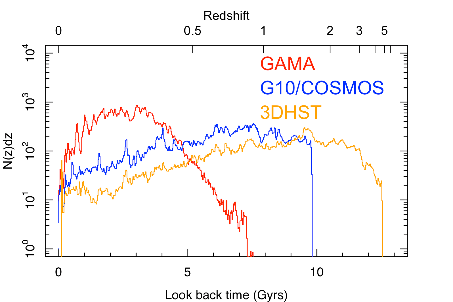
Figure 4: The observed redshift distributions of the final selected GAMA, G10-COSMOS and 3D-HST datasets (as indicated).

3 MAGPHYS Analysis

Here we describe the MAGPHYS fitting process from which we obtain stellar and dust mass estimates and dust corrected star-formation rates. MAGPHYS is an SED fitting code (da Cunha, Charlot & Elbaz 2008) which uses an extensive stellar library based on Bruzual & Charlot (2003) synthetic spectra. Here we elect to use the BC03 libraries rather than the more recent CB07 (Charlot & Bruzual 2007) which arguably over-predicts the Thermally Pulsing-Asymptotic Giant Branch (TP-AGB) phase. The library samples spectra with single (exponentially decaying) star-formation histories over a range of e-folding timescales ($10^{5}-2\times 10^{10}$ yr), and over a broad range of metallicities. Starlight is assumed to be attenuated by both spherically symmetric birth clouds, as well as the ISM using the Charlot & Fall (2000) prescription. The energy lost to dust attenuation is then projected into the mid- and far-infrared assuming four key dust components: PAH and associated continuum, and hot, warm and cold dust components. Sets of optical and far-IR spectra, where the energy lost in the optical equates to the energy radiated in the far-IR, are then regressed against the flux measurements and errors to determine a best fit SED and to determine optimal parameters and probability density functions for the parameters in question. While MAGPHYS produces a wide range of measurements here we focus only on the stellar mass, star-formation rate and dust masses which are considered robust (Hayward & Smith 2015).

The explicit version of the MAGPHYS code that we implement here, has also been adapted by us as follows:

(i) the code has been modified to derive fluxes based on photon energy rather than photon number in the far-IR,

(ii) the latest PACS and SPIRE filter curves are used (in particular the PACS filter curves have changed significantly as the instrument characteristics have become better defined),

(iii) the code has been modified to use upper-limits by identifying zero flux as a limit and using the error as the upper-bound,

(iv) we have extended the upper limit for the output dust mass probability density distribution, from $10^{9}$ to $10^{12}$M_⊙ as a small number of systems were hitting the $10^{9}$M_⊙ upper buffer.

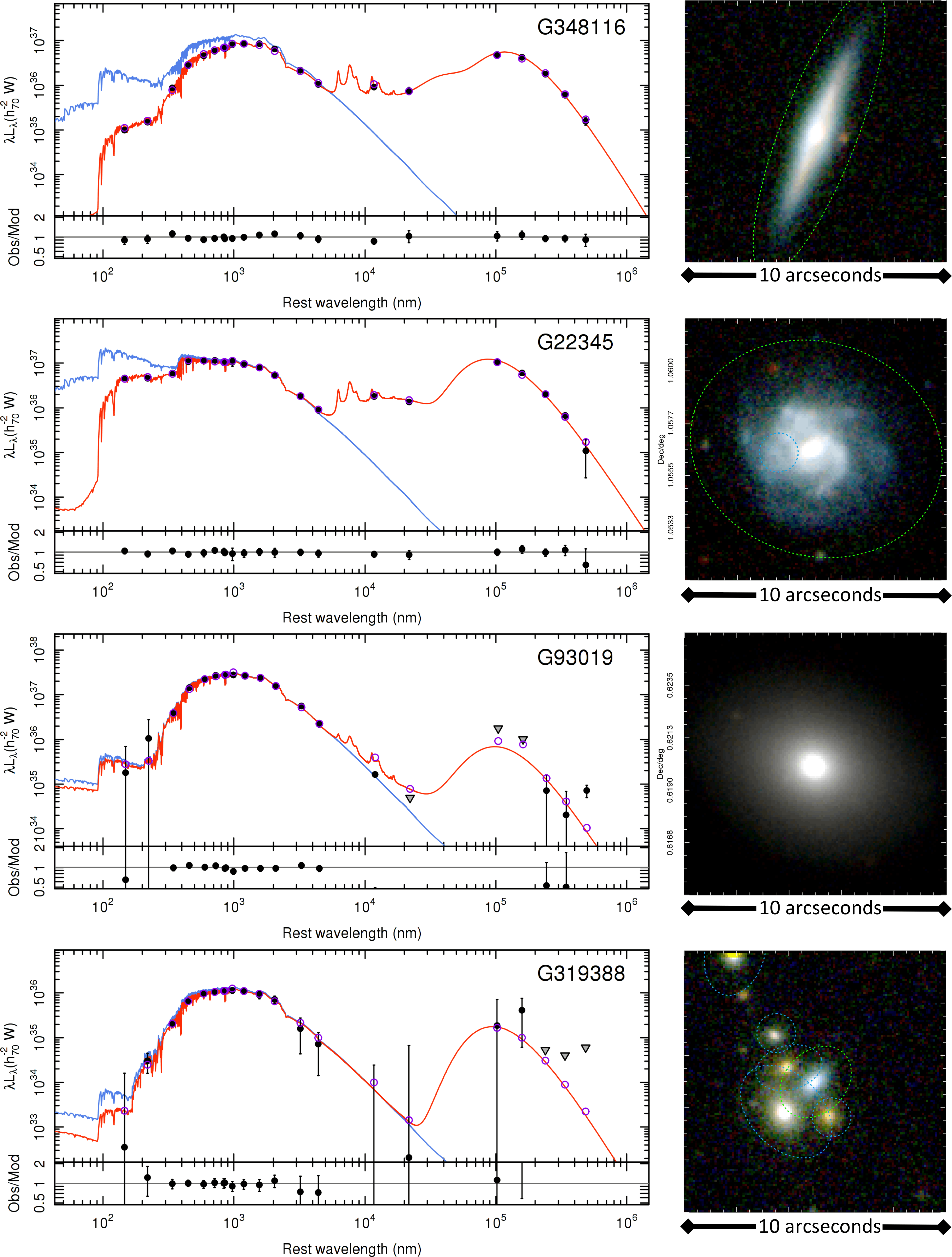
Figure 5: Four examples of GAMA galaxies at $z\approx 0.1$ processed with MAGPHYS. The left panels show the spectral energy distributions showing the data points (black circles), limits (triangles) and the dust attenuated (red curve) and dust unattenuated (blue) MAGPHYS fits, with residual values shown at the bottom. The right side panels show a $KZr$ images from VISTA/VIKING and SDSS, the green dotted ellipses denote the apertures used by LAMBDAR.

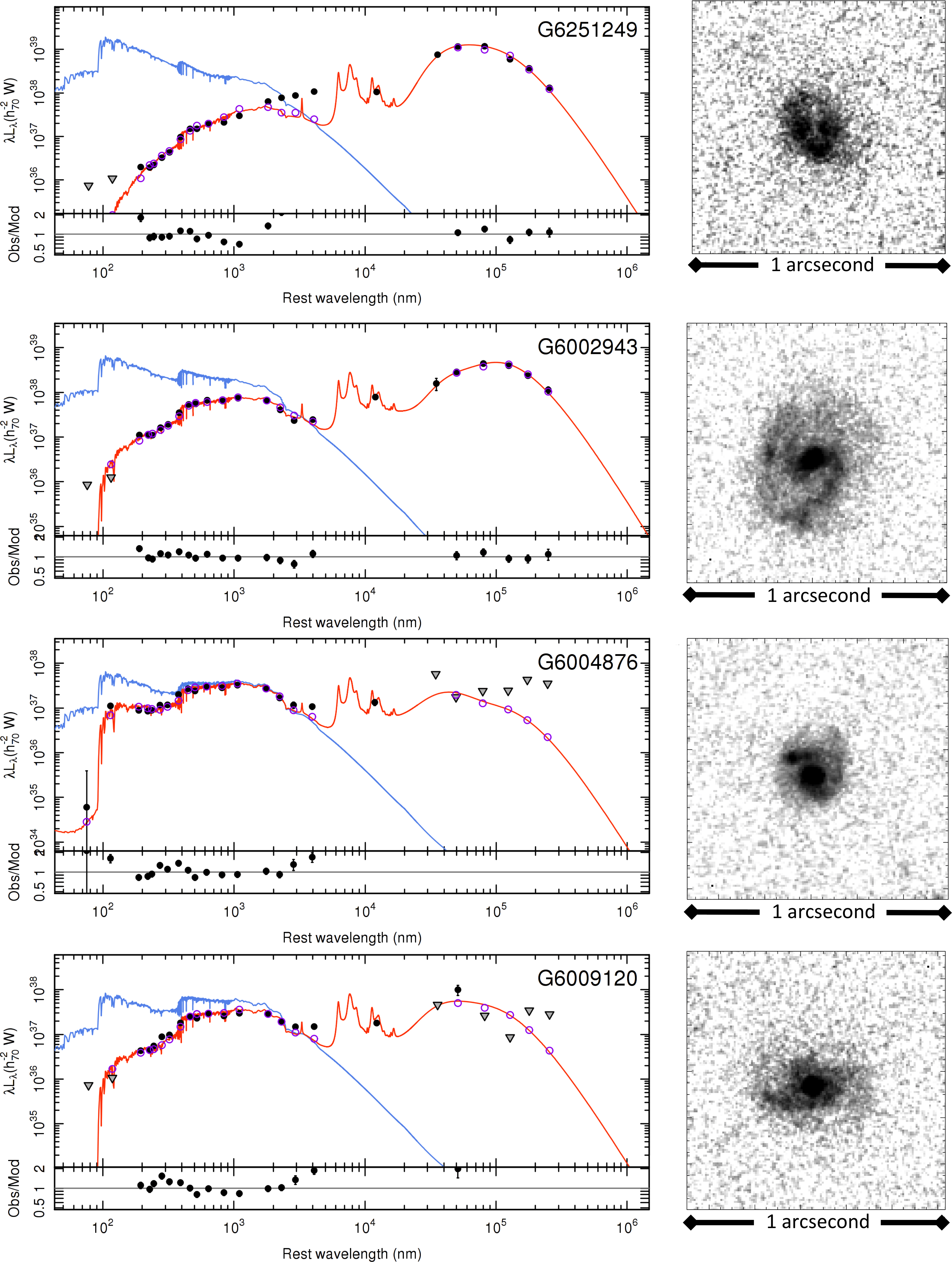
Figure 6: Four examples of G10-COSMOS galaxies at $z\approx 1$ processed with MAGPHYS. The left panels show the spectral energy distributions showing the data points (black circles), limits (triangles) and the dust attenuated (red curve) and dust unattenuated (blue) MAGPHYS fits, with residual values shown at the bottom. The right side panels show the HST F814W image ($2^{\prime}\times 2^{\prime}$). Note the top panel shows a system with strong AGN contamination.

3.1 Data preparation

The GAMA, G10-COSMOS and 3D-HST datasets are as described in Sections 2.1, 2.2 and 2.3 respectively. Critically the GAMA and G10-COSMOS panchromatic catalogues are based on LAMBDAR analysis (Wright et al. 2016) which produces either flux measurements with errors, upper-limits, or provides a flag (-999) for objects where there is no imaging coverage in that filter. The 3D-HST data is obtained from the public download site (See (http://3dhst.research.yale/edu/Data.php and associated documentation). The MAGPHYS code is capable of managing three types of data: MEASUREMENTS: positive flux and positive flux error; LIMITS: zero flux and positive flux-error; NODATA: negative flux values.

For GAMA: Our earlier LAMBDAR analysis provides appropriate values by default for all 128,568 galaxies in the common coverage region, i.e., every galaxy contains flux measurements in all far-IR bands using the r-band optically defined aperture convolved with the appropriate instrument PSF. See Wright et al. (2016) for full details of these measurements.

For G10-COSMOS: In the Andrews et al. LAMBDAR analysis of G10-COSMOS data we adopted a cascading selection in the far-IR to manage the extreme mismatch in depth between the optical selection band and the far-IR Spitzer and Herschel data. In the case of objects with non-measurable fluxes in Spitzer 24 $\mu$m, these were not propagated for measurement at longer-wavelengths. This process was replicated as the analysis progressed to longer wavelengths. For objects excluded via this process, and for which LAMBDAR measurements were therefore not made, we set the flux limits to zero and adopt a flux-error equivalent to the quoted $1\sigma$ point-source detection limit appropriate for each band (see Andrews et al. 2017a, figure 2).

Following the initial analysis a number of systems were identified with predicted fluxes above the detection threshold. This then led to a modified selection and additional flux measurements which expanded our far-IR measurements from $\sim$12k systems to $\sim$24k systems and is outlined in Appendix A. This revised LAMBDAR catalogue was then prepared and passed through MAGPHYS to generate our final G10-COSMOS MAGPHYS catalogue (again see Appendix A for further details).

For 3D-HST: We extracted the following filter combinations from the panchromatic catalogues provided online by the 3D-HST team:

AEGIS: $u,g,F606W,r,i,F814W,z,F125W,j1,j2,j3,j,$ $F140W,h1,h2,h,F160W,k,ks,irac1,irac2,irac3,irac4$

COSMOS: $u,b,g,v,F606W,r,rp,i,ip,F814W,z,zp,Y_{VISTA}$ $F125W,j1,j2,j3,j,J_{VISTA},F140W,h1,h2,H,H_{VISTA}$ $F160W,k,ks,Ks_{VISTA},irac1,irac2,irac3,irac4$

GOODS-N: $u,F435W,B,V,F606W,r,F775W,z,F850LP$ $F125W,j,F140W,h,F160W,ks,irac1,irac2,irac3,irac4$

GOODS-S: $u38,u,F435W,b,v,F606WC,F606W,r,rc,F775W$ $i,F814W,F850LP,F850LPc,F125W,j,j_{tenis},F140W,h$ $F160W,k_{tenis},ks,irac1,irac2,irac3,irac4$

UDS: $u,B,V,F606W,r,i,F814W,z,F125W,j,F140W,h$ $F160W,ks,irac1,irac2,irac3,irac4$

For the 3D-HST data no limits are used, i.e., all measurements either have an appropriate measurements or no data recorded. and grism or photometric redshifts for all objects.

3.2 Processing 600,000 files using the MAGNUS Supercomputer

To optimise the processing of multiple runs of $\sim 600,000$ independent galaxies we developed a Python script which sorted the galaxies by redshift (rounded to four decimal places) and batch ran galaxies with redshifts within $\pm 0.0001$ intervals using the pre-prepared MAGPHYS libraries. This essentially provided a speed-up factor of $\times 10$ over regenerating redshifted SED libraries for each individual galaxy.

The MAGPHYS SED fitting was run on the Magnus machine at the Pawsey Supercomputering Centre. Magnus is a Cray XC40 Series Supercomputer made up of 1,488 compute nodes. Each node contains twin Intel Xeon E5-2690V3 Haswell processors (12-core, 2.6 GHz), and has 64GB of DDR4 RAM. Jobs are then submitted using the SLURM (Yoo et al. 2003) job scheduler. In effect Magnus is therefore running MAGPHYS independently across 35,712 processors. With this capacity we are able to process all 600,000 systems within a 24 hr period. In total the MAGPHYS runs were performed approximately six times for each dataset, as improvements were made in the photometry during LAMBDAR development and updates to the MAGPHYS code (as described) or the FILTERBIN.RES file.

For 3D-HST we run both the standard MAGPHYS template library, and the high-z MAGPHYS template library on all data and use the $\chi^{2}$ values returned by MAGPHYS to select whether to adopt the standard or high-z results. In 97 per cent of cases the optimal fit is selected from the standard-MAGPHYS output rather than the high-z template set.

The MAGPHYS process, as described above, provides star-formation, stellar mass, and dust mass estimates for every galaxy within our optically flux selected samples. For GAMA, G10-COSMOS and 3D-HST these selection limits are: $r<19.8$ mag, $i\leq 25$ mag and $F814W\leq 26.0$ mag respectively (see Section 2), and these are the only relevant selection limits. In all other bands measurements have been made, using the optically defined apertures, except for G10-COSMOS-only where far-IR measurements are made for the 24k objects, with the brightest predicted 250$\mu$m flux, and upper limits assigned to the remainder. For those G10-COSMOS systems with assigned far-IR upper-limits the dust mass estimates essentially revert to an estimated dust mass based on the Charlot & Fall (2000) prescription.

3.3 Diagnostics and verification

Fig. 5 shows four examples of the GAMA MAGPHYS outputs. These examples are relatively bright galaxies extracted from the GAMA sample and have been selected to illustrate an edge-on spiral, a face-on spiral, an elliptical, and a crowded field system. In all cases the MAGPHYS fits, indicated by the unattenuated (blue) and attenuated (red) lines, are reasonable, and the residuals are small, indicating plausible fits. As expected the two spirals have far-IR peaks which are as prominent as their optical peaks, whereas the elliptical galaxy shows a more suppressed far-IR peak — presumably due to a paucity of dust. As a consequence the attenuated and unattenuated curves are very similar for the elliptical galaxy — what you see is what you get — whereas for the spirals the actual energy production is significantly higher than the optical light would indicate, i.e., spiral galaxies are heavily obscured. The edge-on spiral is significantly more attenuated than the face-on spiral, again as one would expect, and highlights the inclination dependence of dust attenuation (Driver et al. 2007). The lower panel, shows an object in a crowded region, and indicates how the LAMBDAR photometric errors inflate where flux has been divided, particularly for those datasets with poorer spatial resolution (i.e. GALEX, WISE and in particular Herschel). The grey inverted triangles indicate bands where the flux measurement is found to be less than the flux error, and hence the flux error becomes the upper limit. Equivalent panels for all GAMA galaxies are available from the GAMA database.

Fig. 6 shows an equivalent set of four galaxies drawn from the G10-COSMOS sample at $z\approx 1$. Again we have selected four galaxies. The first illustrates likely AGN contamination and excessive far-IR emission, the second a face-on spiral but one which is clearly dustier than the low-z counterpart, and two examples of galaxies where upper limits are in play.

In addition to the systems shown in Figs. 5 & 6 individual inspections were made of several hundred objects drawn randomly from each dataset. In the vast majority of cases ($>99$ per cent) the MAGPHYS outputs appear appropriate and the attenuated data accurately describe the measured flux values.

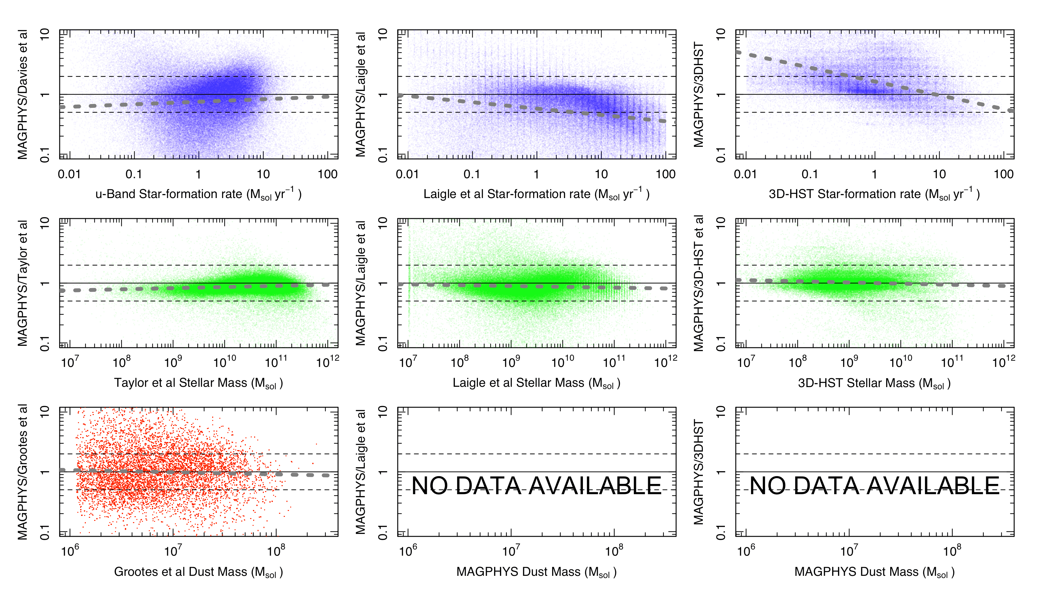
Figure 7: (upper panels) Comparisons between the star-formation rates estimated from the literature to our MAGPHYS measurements for GAMA left), G10-COSMOS (middle panels), and 3D-HST (right). (middle panels) Comparisons between stellar mass estimates from the literature to our MAGPHYS measurements for GAMA and (lower panels) comparisons between dust mass estimates from Grootes et al. (2013) to our MAGPHYS GAMA measurements. In each panel we show a $times2$ deviation as dotted lines and the fitted linear trend.

3.4 Cross-checking measurements

Demonstrating the veracity of the full sample is non-trivial, however, we can compare the MAGPHYS derived stellar and dust masses, and dust corrected star-formation rates, to those derived via other methods/groups. In particular all three samples, GAMA, G10-COSMOS and 3D-HST, have published stellar mass estimates and star-formation estimates (see Table. 2). Fig. 7 shows a comparison of the MAGPHYS measurements derived as described in section 3, to the available star-formation rates (upper), stellar-masses (middle), and dust masses (lower), for the GAMA (left), G10-COSMOS (centre), and 3D-HST (right) samples.

Table 2: Literature references against which we compare our stellar masses and cosmic star-formation rates

Dataset	Stellar Masses	Dust Masses	Star-formation rates
GAMA	Taylor et al. (2011)	Grootes et al. (2013)	Davies et al. (2016)
G10-COSMOS	Laigle et al. (2016)	N/A	Laigle et al. (2016)
3D-HST	Skeleton et al. (2013)	N/A	Momcheva et al. (2016)

On Fig. 7 the parity line is indicated in solid black and variations of $\times 2$ by the dotted tram-lines. The thicker dashed line shows a robust linear fit to the data. In the upper panels of Fig. 7 we compare the star-formation estimates. Note that these are derived in distinct ways. The star-formation rates for our GAMA and G10-COSMOS samples are based on UV-far-IR SED template fitting (da Cunha, Charlot & Elbaz 2008) and hence include an individual dust correction for each galaxy. The estimate of Davies et al. (2016) for GAMA relies on the calibration of $u$-band fluxes to the late-type disk sample of Grootes et al. (2013) which used full radiative transfer modelling. The G10-COSMOS values are taken from the catalogue provided by Laigle et al.(2016). The 3D-HST values are from Whitaker et al. (2014) via FAST (Kriek et al., 2009) fitting.

A fairly significant trend is seen between our MAGPHYS star-formation measurements for 3D-HST compared to their published values. The trend is in the sense that MAGPHYS star-formation rates are higher than 3D-HST at lower star-formation rates. There is also a cloud of outliers which may arise from some inconsistency in the photometry across the bands. For example, and particularly in the COSMOS region, we see some inconsistencies between the CFHT and Subaru photometry. This argues for the need at some point to revisit the 3D-HST photometry using a LAMBDAR-like method to homogenise aperture measurements across all the bands. At this point we elect to move forward with the MAGPHYS star-formation measurements for all three datasets to ensure that our measurements are based on a consistent methodology, IMF, and dust assumptions.

In the middle panels of Fig. 7 the stellar mass estimates show reasonably good agreement across all three datasets, mild trends are seen but clearly the bulk of the population have stellar mass estimates well within the dotted lines. This suggests a high level of consistency across the three datasets.

On Fig. 7 (lower left) we compare the MAGPHYS derived dust masses to those derived by Grootes et al. (2016) using a full radiative transfer treatment. This is a sample of 6356 late-type spiral field galaxies, introduced in Grootes et al. (2013), where the $\tau$ opacity values were derived. Note that in order to make a valid comparison we correct the Grootes et al. data from an emissivity based on Weingartner & Draine (2001) to that adopted by MAGPHYS, requiring an upward modification of the Grootes et al. dust masses by 40%. While the comparison shows scatter the fitted robust linear fit (thick grey dashed line) shows extremely good agreement of the mean behaviour with no obvious bias with mass. We note that the Grootes et al. data has an associated error of $\pm 0.2$ dex suggesting that the majority of the error seen is coming from the MAGPHYS data with a 1$\sigma$ error of $\pm 0.3$ dex in the MAGPHYS dust mass estimates. This is in good agreement with the findings of Beeston et al. (2017) who see a MAGPHYS error ranging from 0.09 dex to 0.5 dex depending on whether the GAMA data contain measurements or upper-limits in the far-IR bands. Unfortunately no literature data currently exists for the G10-COSMOS region but is work in progress by a number of teams.

Figure 8: A comparison of star-formation rates, stellar mass measurements and dust mass measurements for $\sim 6000$ galaxies in common between our G10-COSMOS and 3D-HST samples.

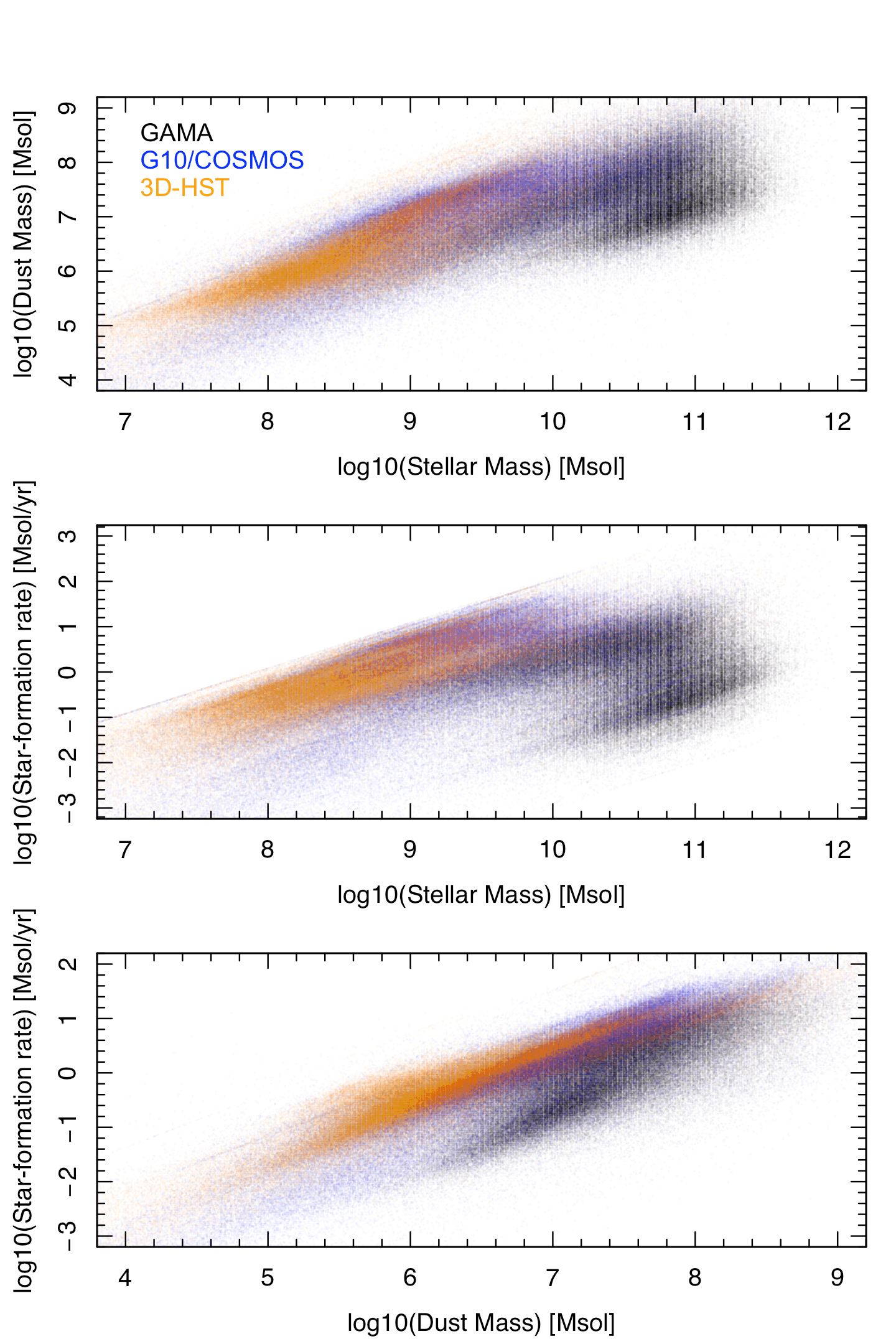
Figure 9: Panels showing the three 2D projections of the 3D cube defined by stellar mass, dust mass, and star-formation rate (our key derived quantities), for each of our three datasets (as indicated). Some striations, binning and boundaries are evident (but not considered problematic), as is a separable high stellar mass, inert, and low dust population at low redshift which we take to be the Elliptical, lenticular and early-type systems. Note that these panels shows the samples in their entirety which span the full redshift range from nearby to $z=5$.

We can also undertake an internal consistency check as one of the five 3D-HST fields lies within the G10-COSMOS region. Using a 0.5^′′ radial match we find 6198 objects from the 3D-HST sample which match our independent G10-COSMOS data. Fig. 8 compares the derived star-formation rates, stellar mass measurements, and dust mass measurements. We find close agreement across all three values with the majority of data points well within the dashed buffer lines. Note that for the 3D-HST derived dust masses no actual far-IR information is included at all.

Finally Fig. 9 shows 2D projections of the 3D-cube defined by our key derived quantities: stellar mass, dust mass, and star-formation rate. The entirety of the three datasets are shown which span the full redshift range. In general the three populations interleave and this is despite the lack of far-IR data constraining the dust masses for 3D-HST. Most obvious is the separable high stellar mass intermediate to low dust mass and inert population in the GAMA sample only (i.e., at low redshift only). We take this population to correspond to elliptical systems known to be mostly devoid of dust with low star-formation rates. In future papers we will explore various trends and scaling relations for the combined dataset as a function of redshift.

Following the above we conclude that we now have consistent and reasonable stellar mass and star-formation rate estimators across the three catalogues extending from $z=0$ to $z=5$.

4 The cosmic star-formation history and the build up of stellar mass and dust mass

Fig. 10 shows the resulting distribution of star-formation (upper), stellar-mass (middle), and dust-mass (lower) measurements. Combined these data cover a significant portion of the star-formation-redshift, stellar-mass-redshift, and dust-mass-redshift planes with each dataset essentially dominating a distinct portion of the parameter space. For GAMA all data have secure redshifts. For G10-COSMOS we highlight those systems with redshifts in light blue and those with photometric-redshifts in mauve (as indicated). The 3D-HST data are shown as photometric redshifts throughout however it is worth noting that both the G10-COSMOS and 3D-HST have quoted photometric errors of $\Delta z<<\pm 0.01$.

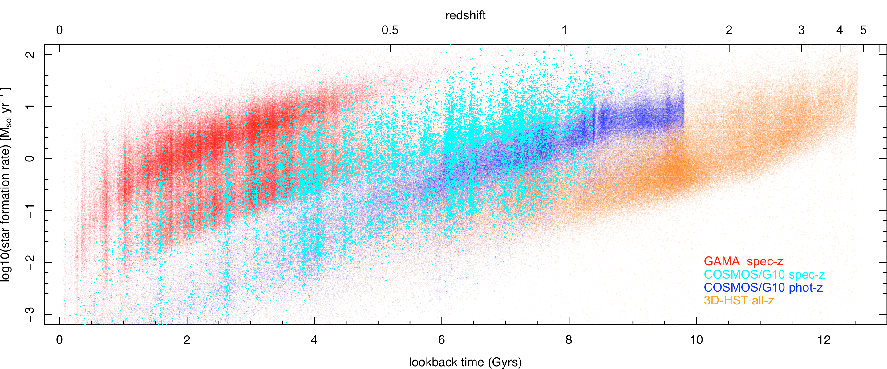
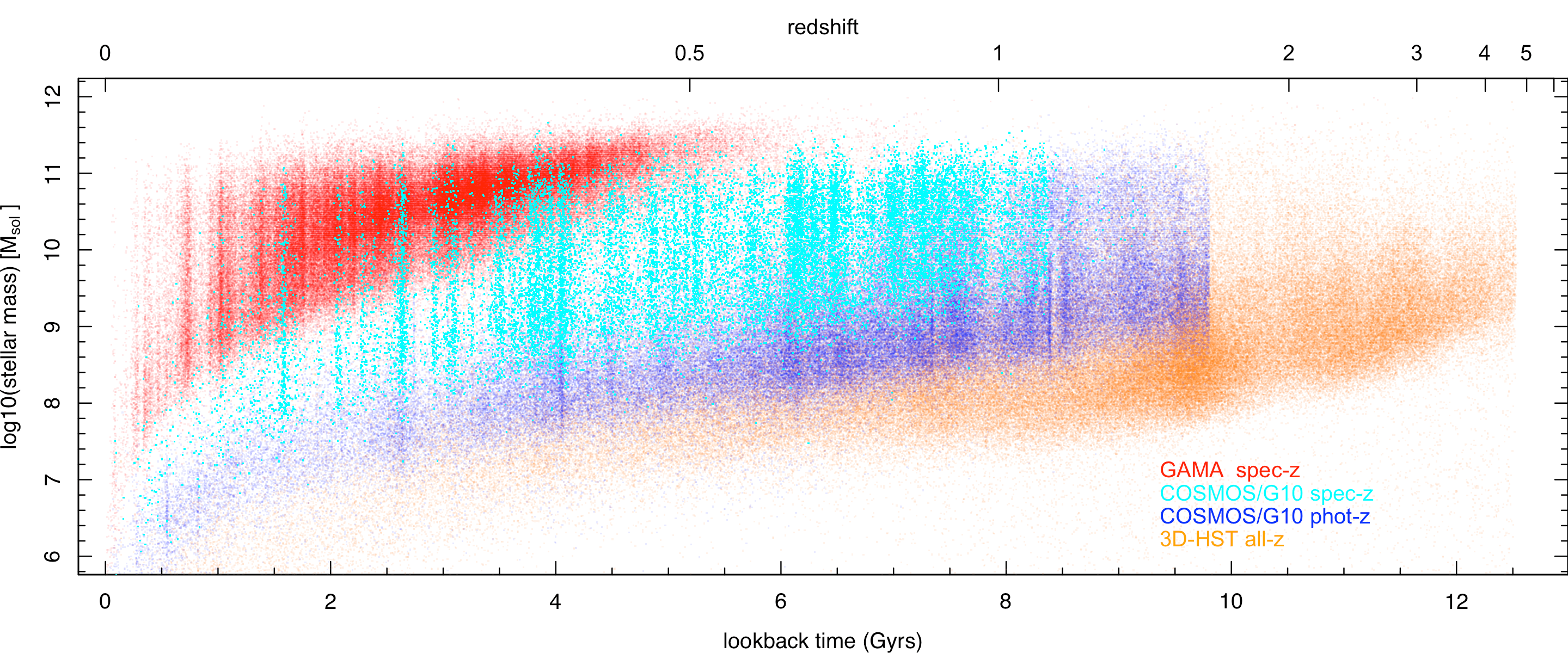
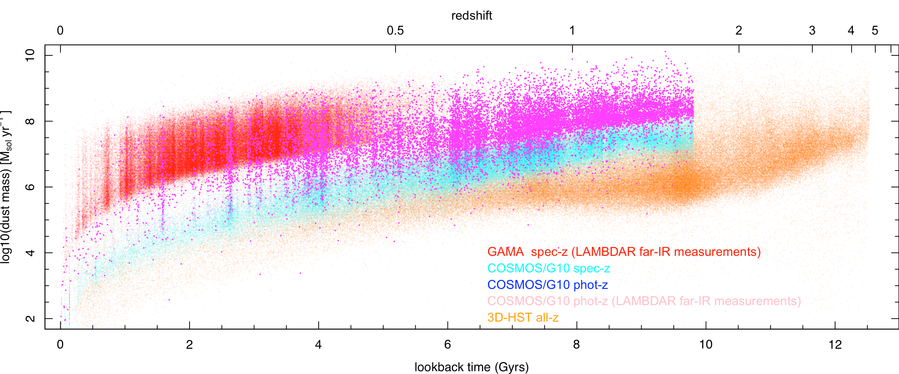
Figure 10: (upper) The star-formation v redshift distributions for the three samples. (middle) The stellar mass redshift distribution of our three complementary samples. (lower) The dust mass redshift distribution for the GAMA and G10-COSMOS datasets.

Of equal interest to the measurements themselves are the quoted error values. Fig. 11 shows the histogram of errors for each dataset and for each of our three key parameters. These errors are directly extracted from the MAGPHYS output and show half the 84 to 16 percentile ranges. For the star-formation rate (top panel) we see a fairly uniform median error of approximately 0.1—0.2 dex for all three datasets. However the GAMA distribution is clearly bimodal which is reflecting the inherent bimodality seen, and well known in the low-z galaxy population, i.e., star-formation rates for early-types have a much broader error range. This bimodality is not apparent in either the G10-COSMOS and GAMA datasets where the incidence of truly inert systems is significantly less, although both the 3D-HST and G10-COSMOS data show long tails towards large error values. For the stellar mass measurements we also see very consistent error distributions of about 0.1 dex, this error range is narrow in keeping with the trends seen in Fig. 7 (middle panels). Finally the lower panel shows the dust mass measurements errors which are significantly broader with median errors of 0.4 and 0.55 for GAMA, and G10-COSMOS. Note because of the lack of far-IR measurements we do not attempt to use the 3D-HST dust mass estimates. The GAMA distribution is again broad and bimodal reflecting those systems for which we have good high signal-to-noise measurements in the far-IR and those for which we have upper-limits only (i.e., $F_{\rm IR}<\Delta F_{\rm IR}$). Recently Beeston et al. (2017) explicitly explored the impact on the dust mass estimate as one reduces from three to zero far-IR filters (see Beeston et al. 2017, their figures 1 & 2), finding that while the dust mass error increases (from 0.09 dex to 0.5 dex), there is no obvious systematic bias. The range of errors found by Beeston matches well the range of recovered measurement errors shown in Fig. 11). Similarly the G10-COSMOS data, for which far-IR measurements exist for a small fraction (10-20 percentile), also has an error that is consistent with the findings of Beeston et al.

The range and spread of these errors shown in Fig. 11, have two important implications. One is that the data will be prone to Eddington bias, particularly for the dust measurements, because the errors are comparable or larger to our adopted bin sizes in the upcoming analysis presented in section 4.1 (0.5 dex for stellar and dust masses). Secondly, a full Monte-Carlo analysis will be necessary because of the spread in errors, i.e., adopting a single error for each parameter, for each datasets, would not be appropriate.

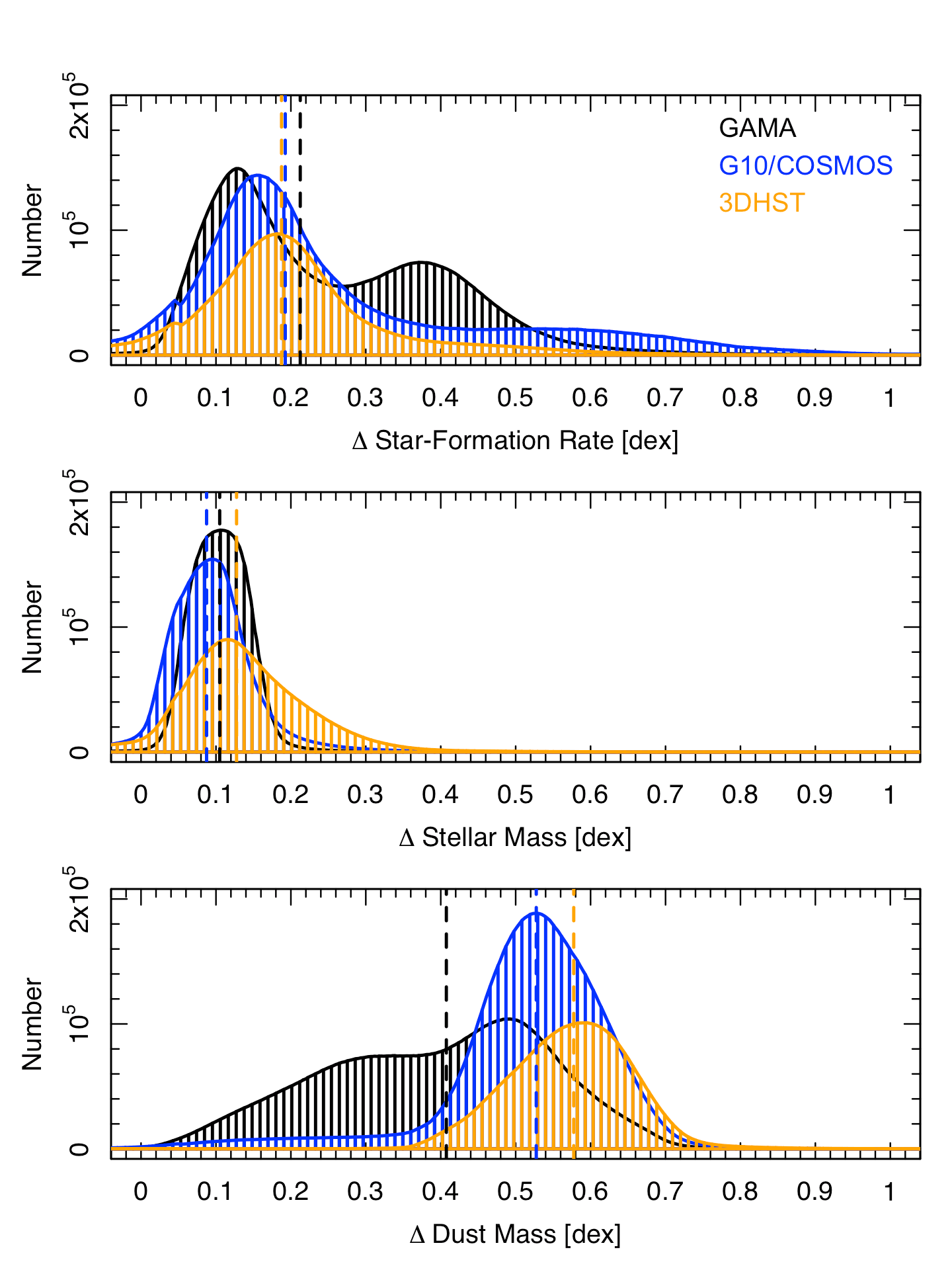
Figure 11: The MAGPHYS errors on each of our three key measurements for our three samples. The MAGPHYS errors are determined from the 84 to 16 percentile ranges.

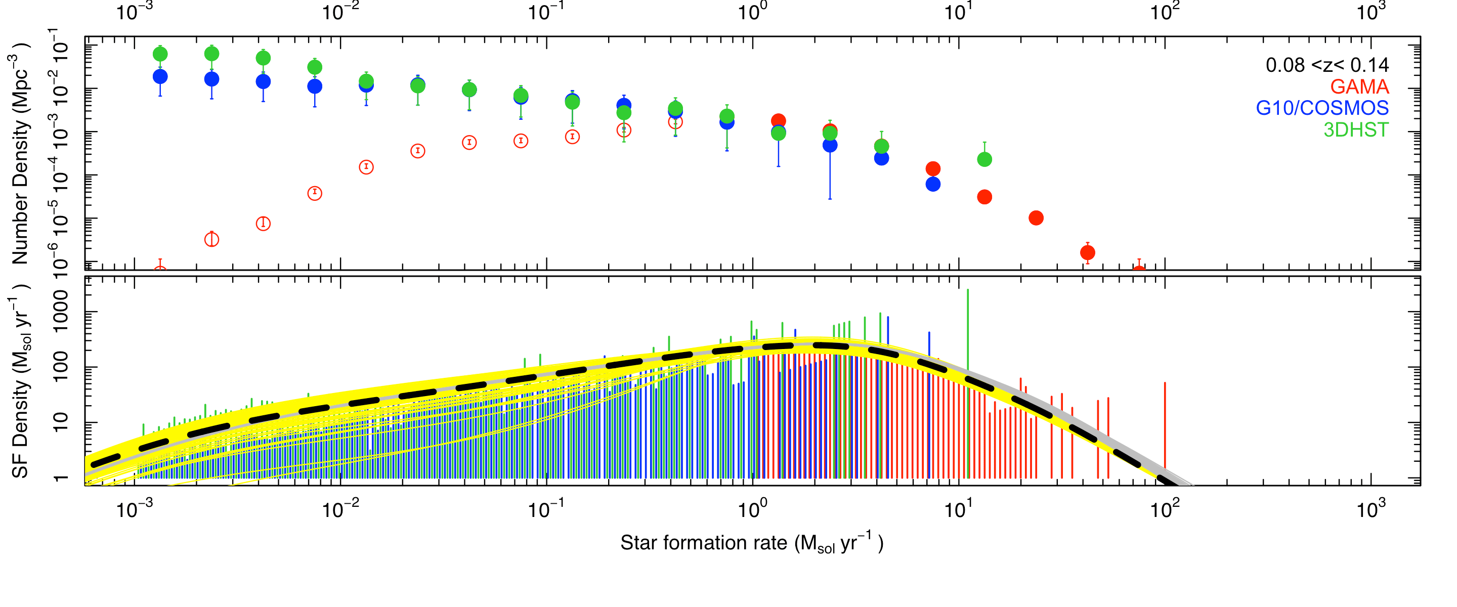
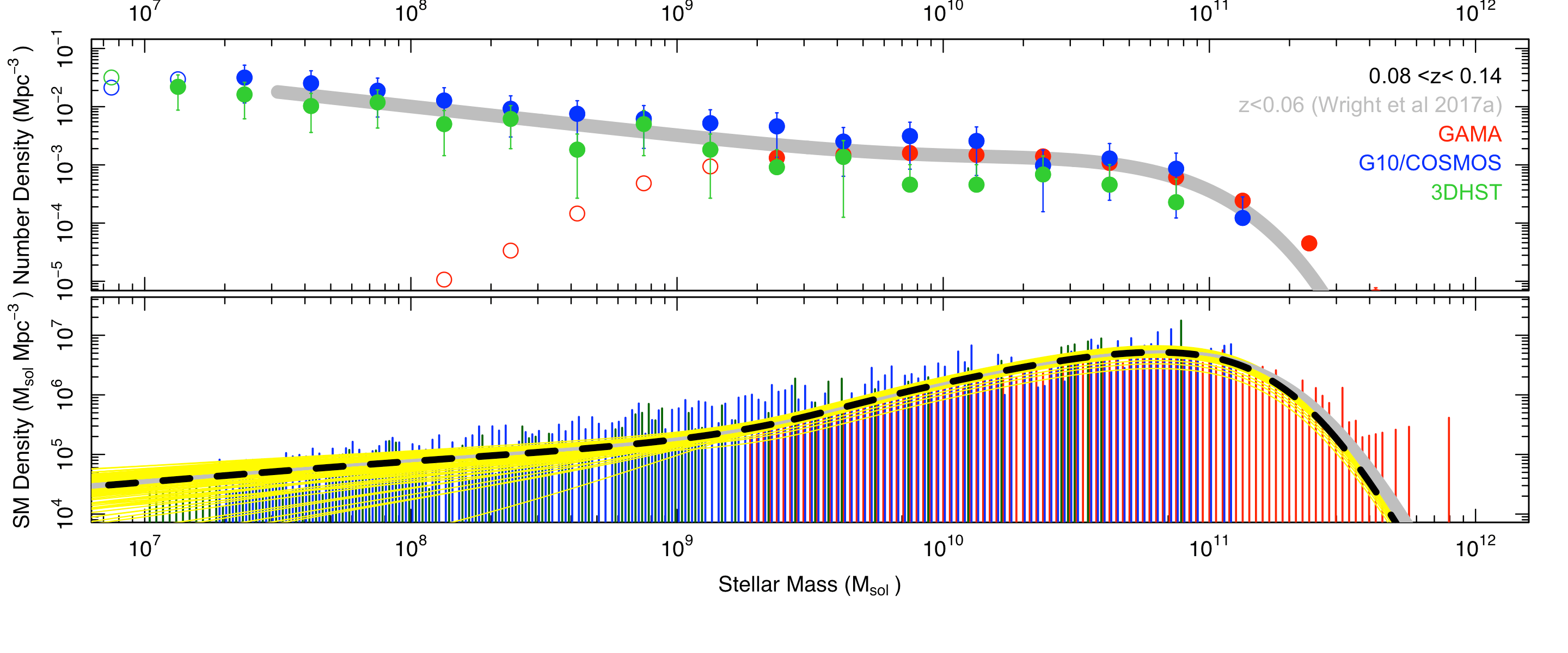
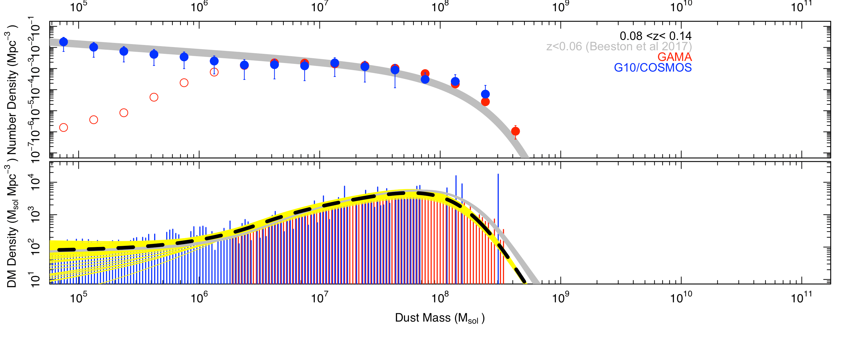
Figure 12: (upper) The star-formation number and density distributions for the GAMA, G10-COSMOS and 3D-HST datasets. (middle) The stellar mass number and density distributions for the GAMA, G10 and 3D-HST samples, (lower) the dust mass number and density distributions for the GAMA and G10-COSMOS samples. In each panel the upper portion shows the number-density without any volume corrections. Data points are plotted in solid if the data are deemed to sample the full volume limited region, and as open symbols if deemed to sample only a fraction of the volume. The thick grey shaded line shows the zero redshift fits determined by Wright et al (2017b) for the galaxy stellar mass function, or by Beeston et al (2017) for the zero redshift dust mass function. In the lower portion of each panel we show the contribution of each interval to the overall SFH, SMF, or DMF. It is this distribution which we fit with a 9-point spline (dashed black line) and integrate to recover the total CSFH, SMD or DMD for that redshift interval. Note that the grey lines represent our Monte Carlo reruns where we modify each galaxy by its individual error (highlighting the Eddington Bias), and the yellow lines represent our Monte Carlo reruns where we perturb each dataset by the estimates cosmic variance error (see Section 4.2 for our error analysis discussion).

4.1 Methodology for deriving star-formation and mass densities

Fig. 12 illustrates our methodology for deriving star-formation (upper), stellar mass (middle), and dust mass (lower) densities in the redshift interval $0.08<z<0.14$. For each redshift interval, we start by constructing the star-formation, stellar mass, or dust mass space-density histograms; having first divided by the appropriate survey volume (where we take the survey areas to be: 117.2 sq deg for GAMA, 1.022 sq deg for G10-COSMOS, and 0.274 sq deg for 3D-HST, see Table. 1). These space-density distributions are shown in the upper half of each panel and constitute the star-formation, stellar mass, or dust mass distributions respectively for a particular redshift slice. No volume corrections are applied and so for each sample the measurements are volume-limited at the right-hand side, but as we move downwards in star-formation rate (or mass), the contributing systems are no longer sampled over the full volume range (redshift slice). At this point the distributions will turn-down due to traditional Malmquist bias.

For each dataset in each redshift interval we can identify this turn-down by noting where the shallower dataset (e.g., GAMA) deviates below the deeper dataset (e.g., G10-COSMOS or 3D-HST). For 3D-HST we simply assume that any sharp downward deviation at low star-formation rate, or low masses is unphysical, and therefore caused by the diminishing volume over which these lower star-forming or lower mass systems are seen. This is a purely empirical constraint and has the distinct advantage of folding in most hidden biases, but the disadvantage of being somewhat subjective. The check comes from the overlap regions between the shallow and deep data.

For example, in the upper-middle panel of Fig. 12 the GAMA stellar mass distribution (red solid points) traces the stellar-mass function down to $\sim 10^{9.5}$M_⊙, at which point the GAMA distribution starts to deviate from the deeper datasets (blue and green points), indicating the onset of incompleteness. We highlight the turn-downs by plotting data which we believe is incomplete using open symbols, and datapoints we consider complete as solid symbols.

To reiterate, in Fig. 12 (upper-middle panel) we see the three stellar mass distributions, where the high-mass end is well defined by the GAMA sample (red symbols), and the intermediate-mass range and low-mass end are well defined by the G10-COSMOS (blue) and 3D-HST (green) samples. As a comparison yardstick the grey curve shows the GAMA Galaxy Stellar Mass Function recently derived by Wright et al. (2017a) for $z<0.1$ which includes a volume correction which incorporates density sampling of the underlying large scale structure. The agreement between the Wright et al. curve and our composite data from the three distinct datasets provides a good demonstration that the G10-COSMOS, 3D-HST data are consistent with the fully volume-corrected low-mass GAMA data.

The lower half of each panel now shows the differential contribution to the star-formation rate (upper), stellar-mass (middle), and dust-mass (lower) densities, i.e., $M\phi(M)dM$ in the stellar mass case. Here the histograms are more finely sampled for plotting clarity and we can see, in the case of stellar mass densities for example, that the peak contribution within this redshift interval occurs at $\sim 10^{10.8}$M_⊙. Again we see how the density distribution is defined by the three distinct datasets with GAMA dominating at high mass (red bars), G10-COSMOS at intermediate mass (blue bars), and 3D-HST at the lowest mass range (green bars). The errors associated with each data point and adopted in the spline fitting (dashed black line) are a combination of Poisson error added in quadrature to the cosmic variance error. The cosmic variance error is derived from Driver & Robotham (2011) and shown in Table 3. We fit a 7-point spline to the full distribution of density spikes weighted by the inverse fractional error squared. Hence the spline most closely follows the GAMA data at high masses, then the G10-COSMOS data and finally the 3D-HST data, i.e., it uses all the data simultaneously but most closely traces the sample with the lowest errors. Finally to determine the overall density we integrate the spline over a fixed star-formation/mass range to get the total density at that redshift.

The use of a spline-fit is necessary, as opposed to just summing the data, because in the higher redshift bins the distribution is only partially sampled. Hence the spline allows us to extrapolate over a fixed star-formation/mass range and to recover star-formation/mass below the detection limits. This introduces the scope for extrapolation error which is managed by the Monte-Carlo error analysis described in the next section. A spline-fit is also preferable to the more standard single or double Schechter function fitting, because it most closely follows the shape of the distributions, however, care must be taken that the spline is well behaved, for this reason we show all our fits in Appendix B (Figs 18 to Fig. B18). Across all bins we can see that the distributions from the three datasets are extremely consistent and well defined. We also note that our technique allows GAMA to remain useful in constraining the highest mass/star-formation end up to $z\approx 0.68$ and G10-COSMOS up to $z\approx 1.75$, with only the 3D-HST data extending to the very highest redshifts $z<5$. The adopted mass and star-formation limits for each dataset, along with the estimated cosmic variance values from Driver & Robotham (2011) are shown in Table 3.

Table 3: A summary of the cosmic variance, stellar mass, dust mass and star-formation limits used in the analysis.

Redshift	GAMA limits				G10-COSMOS limits				3D-HST limits
interval	CV	$M_{\rm*,lim}$	$M_{\rm D,lim}$	$\log_{10}SF_{\rm lim}$	CV	$M_{\rm*,lim}$	$M_{\rm D,lim}$	$\log_{10}SF_{\rm lim}$	CV	$M_{\rm*,lim}$	$M_{\rm D,lim}$	$\log_{10}SF_{\rm lim}$
		$(M_{\odot})$	$(M_{\odot})$	$(M_{\odot}yr^{-1})$		$(M_{\odot})$	$(M_{\odot})$	$(M_{\odot}yr^{-1})$		$(M_{\odot})$	$(M_{\odot})$	$(M_{\odot}yr^{-1})$
$0.02$—$0.08$	0.19	8.75	5.75	-1.00	0.77	6.75	4.00	-3.0	0.60	6.50	4.00	-3.00
$0.06$—$0.14$	0.13	9.25	6.25	0.00	0.59	7.25	4.25	-3.0	0.50	7.00	4.00	-3.00
$0.14$—$0.20$	0.10	10.00	6.50	0.00	0.51	7.50	4.50	-3.0	0.45	7.00	4.50	-3.00
$0.20$—$0.28$	0.072	10.50	7.00	0.25	0.39	7.50	4.75	-2.50	0.40	7.25	5.25	-2.50
$0.28$—$0.36$	0.062	10.75	7.50	0.75	0.35	7.75	5.25	-1.75	0.40	7.50	5.25	-1.75
$0.36$—$0.45$	0.052	11.0	8.50	1.00	0.30	8.00	5.25	-1.50	0.35	7.75	5.25	-1.50
$0.45$—$0.56$	0.043	11.25	9.00	1.50	0.26	8.25	6.00	-1.00	0.30	7.75	5.50	-1.00
$0.56$—$0.68$	0.039	11.50	9.25	1.75	0.23	8.50	6.00	-0.50	0.25	8.00	5.75	-1.00
$0.68$—$0.82$	0.035	11.75	-	-	0.21	8.50	6.25	-0.50	0.20	8.25	5.75	-0.75
$0.82$—$1.00$	0.03	-	-	-	0.18	9.00	6.75	0.00	0.20	8.25	6.00	-0.50
$1.00$—$1.20$	0.03	-	-	-	0.18	9.00	7.00	0.25	0.18	8.50	6.00	-0.50
$1.20$—$1.45$	0.03	-	-	-	0.18	9.25	7.25	0.50	0.18	8.75	6.25	-0.25
$1.45$—$1.75$	0.03	-	-	-	0.18	9.75	7.25	0.75	0.15	8.50	6.25	-0.25
$1.75$—$2.20$	0.03	-	-	-	0.18	-	-	-	0.15	9.25	6.75	0.00
$2.20$—$2.60$	0.03	-	-	-	0.18	-	-	-	0.10	9.25	7.00	0.50
$2.60$—$3.25$	0.03	-	-	-	0.18	-	-	-	0.10	9.50	7.25	0.75
$3.25$—$3.75$	0.03	-	-	-	0.18	-	-	-	0.10	9.50	7.50	0.75
$3.75$—$4.25$	0.03	-	-	-	0.18	-	-	-	0.10	9.50	7.50	1.00
$4.25$—$5.00$	0.03	-	-	-	0.18	-	-	-	0.10	9.50	7.50	1.25

4.2 Measurement and error analysis

We consider three forms of error: that arising from Poisson statistics; that arising from the cosmic variance (see Table 3); and Eddington bias.

To assess the statistical error we jostle all data points individually by drawing randomly from a Normal distribution of width equal to the quoted MAGPHYS measurement error for each galaxy, and then rerun the full analysis and repeat 101 times (sufficiently large to sample the error range but not so large to be computationally challenging). We then assess the spread of each of our derived density values (these alternative fits are shown as the grey lines on the lower panels of Fig. 12). These lines highlight both the resilience to Poisson error, but also the potential impact of any Eddington bias (based on how well the grey lines cluster around the base measurement (given by the dashed black line). In each case the star-formation density, stellar mass density, or dust mass density, is derived from the integrations of the splines. With our base measurement coming from the integration of the dashed black line. We can similarly integrate each of the grey splines to get both the dispersion in measured values (from the 84-16 percentile range), and an offset from the base measurement due to the error perturbation process (the Eddington bias). We correct our derived data for this bias by subtracting the offset of our base measurement from the median of our Poisson re-fits.

To assess the cosmic variance error we again repeat the analysis but this time jostle the amplitude of each of the entire three datasets independently, by drawing from a Normal distribution of width equal to the estimated CV error, as listed in Table 3. Again we repeat the analysis 101 times (yellow lines on Fig.12) and once again assess the dispersion for each of our derived values.

Finally, we rerun our base analysis for our three AGN selections for the 3D-HST dataset (see Section 2.4) representing the lenient, fair, and extreme selections and determine an error estimate based on half the range across the three measurements. Tables 4, 5 & 6 show our final measurements, including the Eddington bias correction, along with each of the individual errors (Eddington bias, Poisson error, CV error, and AGN classification uncertainty).

Note when fitting splines we utilise the information of null data in a high stellar-mass, dust-mass or star-formation bin, where an absence of data represents significant information, by setting the first unoccupied bin to have a low value with high significance, this ensures that the spline fits bound the data at the high mass or star-formation end and do not diverge or include excess extrapolated flux.

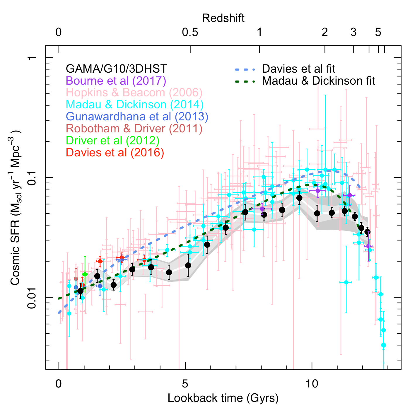
Figure 13: The cosmic star-formation history as a function of lookback time. Shown are literature compendia along with the recently trends reported by Davies et al. (2016) and Madau & Dickinson (2014). Our new measurements from our combined sample are shown in black with the three error components indicated by the distinct grey shading. The errors are shown as additive with the light grey indicating statistical error, the grey as the cosmic variance, and the dark grey the AGN classification uncertainty. Note that a figure showing the same data versus redshift is given in Appendix C. 36.

4.3 The Cosmic Star-formation History

The cosmic star-formation history is one of the most well studied cosmic-planes since the original work from the Canada France Redshift Survey (CFRS; Lilly et al.  1996), and the Hubble Space Telescope Hubble Deep Field (HDF; Madau et al. 1998). Fig. 13 shows two compendia of recent measurements drawing in disparate star-formation tracers from diverse surveys. These compendia are taken from Hopkins & Beacom (2006; light pink), and Madau & Dickinson (2014; cyan). For the genesis of the individual data points please see the Tables included in these works. Note also that the Madau & Dickinson compendium includes many of the Hopkins & Beacom data but corrected for various issues which later came to light (i.e., recalibrations, treatment of $h$ etc). For this reason we show the more recent Madau & Dickinson data in bright cyan and the earlier older Hopkins & Beacom compendium in light pink, an offset between these two compendia is clearly visible. Note we convert from Salpeter (or Salpeter-A) IMFs to Chabrier IMFs by multiplying by a factor of 0.63 (0.85) (see Madau & Dickinson 2014 and Driver et al. 2013). Also obvious is the significant vertical scatter which arises from the use of distinct tracers, and in some cases the relatively small volumes probed giving rise to significant cosmic variance fluctuations.

Also shown are recent measurements at very low redshift (Robotham & Driver 2011; Driver et al. 2012; Gunawardhana et al. 2013; Davies et al. 2015, with the latter four of these coming from various distinct analysis of the GAMA data). Recent fits to the data are shown as either the dashed green line (Madau & Dickinson 2014), or the dashed mauve line (Davies et al. 2016), with Davies et al. finding a very similar but marginally higher SFR due to the inclusion of the Hopkins & Beacom data in the fitting. Finally we show the most recent data from Bourne et al. (2017; purple points) based on SCUBA observations of selected 3D-HST galaxies.

Overlain as solid black discs with error-bars, are data derived from the combined GAMA/G10-COSMOS/3D-HST dataset, produced in the manner described in the previous section. Because of the very large size of the GAMA, G10-COSMOS and 3D-HST datasets the Poisson errors become vanishingly small (light grey shading) and the dominant error comes from cosmic variance (grey shading; particularly at the lower redshift end) and AGN-uncertainty (dark grey shading band; at the high redshift-end). Note, these errors are shown added linearly. We now have a complete record of the star-forming history over a 12 Gyr timeline drawn from the combination of three large datasets with cross-calibrated star-formation rates. Particularly noticeable is that the error spread is now almost a factor of $\times 2$ better than the Madau & Dickinson compendium and $\times 5$ better than the Hopkins & Beacom compendium. Our values agree well with the Madau & Dickinson data, although we do see a modest tendency for our data to lie slightly below the Madau & Dickinson fit, and in particular a slump at  5 Gyrs lookback time ($z\approx 0.5$). Although the Madau & Dickinson compendium is fairly thin on the ground we ascribe this slump to cosmic variance because a similar slump is also seen in the stellar mass density shown in the middle panel. AT high-z we see our data falls below the most recent study of Bourne et al. (2017). There are two obvious possibilities: Either our study is incomplete for highly obscured star-formation, or the Bourne et al. study is contaminated by AGN. Distinguishing between these two possibilities is not trivial and will take significant effort. We therefore elect to carry both our data and the Bourne data forward.

In later analysis where we fit these data we will also fold in the highest seven redshift data points taken from Table 1 of Madau & Dickinson (but originally reported in Bouwens et al. 2012a,b and Schenker et al. 2013), and which extend to 12.8 Gyrs in lookback time (i.e., see Fig. 16 upper panel), in addition to the Bourne et al. (2017) data (purple dots).

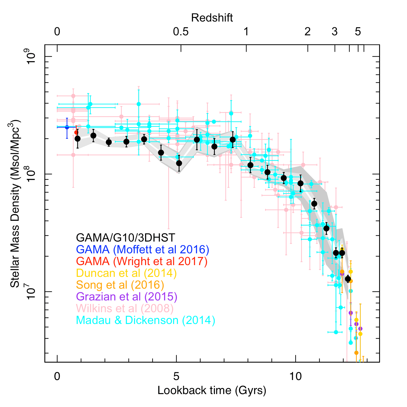
Figure 14: The stellar mass density versus lookback time. Shown are literature compendium and recently measurements along with our measurements form our combined sample (black dots). The grey bands show the error budget, plotted in additive fashion with the light grey representing the statistical uncertainty, the grey line the cosmic variance and the dark grey the uncertainty from AGN classification.

4.4 The build-up of the stellar mass density

Fig. 14 shows the stellar mass density as a function of cosmic time, compared to the Wilkins et al. (2008; light pink data points), and the Madau & Dickinson (2014; cyan) compilations of literature estimates. As before we show the more recent compendium in bright cyan and the older Wilkins et al. compendium in light pink and have scaled down the stellar masses by 0.63 to convert from a Salpeter IMF to a Chabrier IMF. The blue point represents a recent stellar mass estimate based on GAMA for $z<0.06$ by Moffett et al. (2016), and the red point shows the recent estimate by Wright et al. (2017) from an analysis of GAMA to $z<0.1$.

The astute will wonder that given the leftmost black data point and the blue and red are essentially three estimates of the same dataset, why do we see any scatter at all? The answer is in the extrapolation and the Eddington bias. In Moffett et al. the data is sub-divided by component and the disc and little blue spheroid (LBS) components exhibit steep low-mass end slopes which when extrapolated yields additional mass. Similarly the dataset shown here is the only one of the three which includes a formal Eddington bias. The range therefore reflects some of the systematic uncertainty inherent in the methodology.

The black data points within the light grey/grey/dark grey shaded region represent the full GAMA/G10-COSMOS/3D-HST combined dataset which span almost the entire timeline of the Universe. These show good agreement with the existing literature values but with less scatter, and a relatively smooth behaviour in which mass builds very rapidly at early epochs and then more slowly over later epochs (although beware the logarithmic scaling). Very slightly noticeable is the close agreement at high-redshift combined with a slight tendency towards low stellar mass densities at lower-redshift. The 50 per cent point is reached at approximately $9\pm 1$ Gyr lookback time. We also note that slump in data at $z\approx 0.5$ which cannot be physical (i.e., the stellar mass density cannot actually decline and rise this quickly), but is most likely due to cosmic (sample) variance and an underdensity in the G10-COSMOS at this redshift.

The main advantage of the combined dataset comes from two principle factors: the homogeneity of stellar mass estimates across the three datasets, and the size of the samples, bringing the errors to a significantly narrower distribution than the assembled literature values.

Finally we also overlay a number of recent high-redshift literature values (Duncan et al. 2014; Grazian et al. 2015 and Song et al. 2016). These align very closely to our high-redshift data showing a complete record of the build-up of stellar mass from $z=8$ to the present day (i.e, from when the Universe was 1 Gyr old to the present time).

It is also worth noting that our dominant error at high-z is due to uncertainty in the AGN identification (dark grey shading), of course at some point this becomes moot as galaxies are neither AGN or star-forming but both and ultimately effort is needed to separate the AGN-light from the stellar emission prior to determining masses.

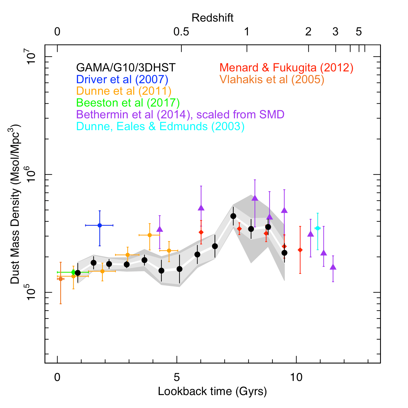
Figure 15: The dust mass density versus lookback time. Shown are various measurements from the literature along with our measurements from the combined GAMA/G10 sample (black dots). The error bands are shown in grey, are additive in indicate the statistical error (light grey), the cosmic variance error (grey), and the error introduced from including objects with or without far-IR measurements (dark grey).

4.5 The recent decline in dust mass density

Fig. 15 shows our recovered dust mass density against lookback time. Initially this trend is flat then rising slowly to $z\sim 1$ with a hint of a decline at our G10-COSMOS redshift limit of $z=1.75$. However, we do not place any significance in this turn-down at $z=1.75$ given the associated errors indicated by the grey shading.

One of the problems in establishing the veracity of this result is that fairly little previous data exists at any redshift. Driver et al. (2008) inferred an estimate from optical data combined with a radiative transfer model, while Dunne et al. (2011) derived measurements from the Herschel-ATLAS Science Definition Phase. Concurrently to this work, an updated measurement of the low-z dust-mass function was obtained by Beeston et al. (2017), also based on the GAMA database and the MAGPHYS data presented here.

Compared to the Driver et al. data we find a marginally (1.5$\sigma$) lower dust mass density than they reported. This is likely due to MAGPHYS recovering significantly lower than expected opacities when compared to the Driver study. In that study a single opacity value was derived and adopted for the entire population ($\tau_{v}^{o}=3.8$ ; Driver et al. 2007). Compared to Dunne et al. our data agree well (all values are within the 1$\sigma$-errors, but rather than seeing a rapidly declining dust mass density we find a relatively flat dust mass density. We note that Dunne et al. raise some concern and caution in using their last data point, without which they concluded a rapidly declining dust density. From an orthogonal analysis of dust lanes in galaxies, Holwerda et al. (2012) also concluded fairly flat evolution of the dust mass density (and its planar distribution) out to $z=1$, supporting our results.

Using mean dust-to-stellar mass ratios for the main sequence reported by Béthermin et al. (2014) we can determine rough values (purple triangles) by scaling our stellar mass densities by these ratios. These were derived from data at wavelengths $>1$mm (i.e., on the Raleigh-Jeans tail to very high redshift) but do implicitly assume that the global dust mass density is very much dominated by main sequence systems rather than extreme burst systems. Also shown are estimates based on MgII absorbers in Quasar sight-lines reported by Menard & Fukugita (2012). Note that these data implicitly assume an SMC-like extinction curve (correcting to a MW-like extinction curve would scale up the data by $\times 1.8$, Gergely Popping priv. comm). The Béthermin and Menard data both agree reasonably well or exceptionally well respectively, with our results painting a consistent picture of the dust density slowly declining over a 10 Gyr period. Finally we include the earlier estimate by Dunne, Eales & Edmunds (2003) based on sub-mm constraints, provide a direct estimate giving a high-z anchor point. From our combined distribution and these supporting data we can make the following statements:

(1) The dust mass density appears to peak around 8 Gyrs ago ($z\sim 1$), suggesting that dust formation is either concurrent with star-formation or lags no more than a few Gyrs behind the star-formation peak (see also Cucciati et al. 2012 and Burgarella et al. 2013). At the current time there is no clear consensus on dust production with advocates for the dominant pathway being SN, AGB, or ISM grain growth (see for example Gall et al. 2014; Sargent et al. 2010; and Rowlands et al. 2014 respectively and references therein). Most likely all pathways are relevant. A Dust Density peak coincident with the CSFH could argue more for the former (i.e., SN which are immediate), over AGB (which would be slightly delayed by as much as 1-2Gyrs), or ISM grain growth which would expect to be a continuous process.

(2) We also see that the total dust mass density declines relatively smoothly over the past 8 Gyrs, implying that in the latter half of the Universe dust is destroyed faster than it is formed (presumably through astration), and the Universe is becoming more transparent. This is also consistent with the reported $A_{FUV}$ evolution in Cucciati et al. (2012) and Burgarella et al. (2013), see also figure 9 of Andrews et al. (2017a). This is not particularly new and unfortunately the current data cannot constrain the key question which is what fraction of the dust is destroyed, whether it is destroyed locally or globally and what fraction might be ejected into the halo or even IGM.

We will return to discuss dust evolution further in Section 6 where we build a simple toy model.

Table 4: Derived cosmic star-formation densities from our combined GAMA/G10-COSMOS/3D-HST sample.

Age$\dagger$	Redshift	Star-formation rate
(Gyr)	interval	$\log_{10}(M_{\odot}yr^{-1}h_{0.7}Mpc^{-3})$
-	-	Value‡	Edd. Bias	$\Delta_{\rm possion}$	$\Delta_{\rm cv}$	$\Delta_{\rm AGN}$
$0.85$	$0.02$—$0.08$	$-1.95$	$0.03$	$\pm 0.00$	$\pm 0.07$	$\pm 0.00$
$1.52$	$0.06$—$0.14$	$-1.82$	$0.03$	$\pm 0.01$	$\pm 0.05$	$\pm 0.01$
$2.16$	$0.14$—$0.20$	$-1.90$	$0.02$	$\pm 0.00$	$\pm 0.04$	$\pm 0.00$
$2.90$	$0.20$—$0.28$	$-1.77$	$0.01$	$\pm 0.00$	$\pm 0.05$	$\pm 0.00$
$3.65$	$0.28$—$0.36$	$-1.75$	$0.01$	$\pm 0.00$	$\pm 0.06$	$\pm 0.01$
$4.35$	$0.36$—$0.45$	$-1.79$	$0.01$	$\pm 0.01$	$\pm 0.06$	$\pm 0.01$
$5.11$	$0.45$—$0.56$	$-1.73$	$0.04$	$\pm 0.01$	$\pm 0.09$	$\pm 0.03$
$5.86$	$0.56$—$0.68$	$-1.56$	$0.05$	$\pm 0.00$	$\pm 0.07$	$\pm 0.02$
$6.59$	$0.68$—$0.82$	$-1.42$	$0.06$	$\pm 0.01$	$\pm 0.06$	$\pm 0.04$
$7.36$	$0.82$—$1.00$	$-1.29$	$0.05$	$\pm 0.00$	$\pm 0.07$	$\pm 0.01$
$8.11$	$1.00$—$1.20$	$-1.31$	$0.04$	$\pm 0.00$	$\pm 0.05$	$\pm 0.01$
$8.82$	$1.20$—$1.45$	$-1.27$	$0.03$	$\pm 0.00$	$\pm 0.06$	$\pm 0.02$
$9.50$	$1.45$—$1.75$	$-1.17$	$0.02$	$\pm 0.00$	$\pm 0.06$	$\pm 0.03$
$10.21$	$1.75$—$2.20$	$-1.30$	$0.04$	$\pm 0.01$	$\pm 0.07$	$\pm 0.06$
$10.78$	$2.20$—$2.60$	$-1.29$	$0.04$	$\pm 0.01$	$\pm 0.04$	$\pm 0.09$
$11.29$	$2.60$—$3.25$	$-1.28$	$0.04$	$\pm 0.01$	$\pm 0.04$	$\pm 0.11$
$11.69$	$3.25$—$3.75$	$-1.33$	$0.03$	$\pm 0.01$	$\pm 0.03$	$\pm 0.08$
$11.95$	$3.75$—$4.25$	$-1.42$	$0.04$	$\pm 0.04$	$\pm 0.05$	$\pm 0.02$
$12.19$	$4.25$—$5.00$	$-1.45$	$0.03$	$\pm 0.04$	$\pm 0.04$	$\pm 0.04$

$\dagger$ The age of the Universe at the volume midpoint of the redshift interval.

$\ddagger$ Note that these values have had the Eddington Bias (given in Col. 4) subtracted from the initial measurement, i.e., they are Eddington Bias corrected.

Table 5: Derived cosmic stellar mass densities from our combined GAMA/G10-COSMOS/3D-HST sample.

Age$\dagger$	Redshift	Stellar mass density
(Gyr)	interval	$\log_{10}(M_{\odot}h_{0.7}Mpc^{-3})$
-	-	Value$\ddagger$	Edd. Bias	$\Delta_{\rm possion}$	$\Delta_{\rm cv}$	$\Delta_{\rm AGN}$
$0.85$	$0.02$—$0.08$	$8.30$	$0.01$	$\pm 0.01$	$\pm 0.08$	$\pm 0.00$
$1.52$	$0.06$—$0.14$	$8.33$	$0.01$	$\pm 0.00$	$\pm 0.05$	$\pm 0.00$
$2.16$	$0.14$—$0.20$	$8.27$	$0.02$	$\pm 0.00$	$\pm 0.03$	$\pm 0.00$
$2.90$	$0.20$—$0.28$	$8.28$	$0.00$	$\pm 0.00$	$\pm 0.04$	$\pm 0.00$
$3.65$	$0.28$—$0.36$	$8.30$	$-0.01$	$\pm 0.00$	$\pm 0.04$	$\pm 0.00$
$4.35$	$0.36$—$0.45$	$8.18$	$-0.01$	$\pm 0.00$	$\pm 0.06$	$\pm 0.01$
$5.11$	$0.45$—$0.56$	$8.09$	$-0.01$	$\pm 0.00$	$\pm 0.07$	$\pm 0.02$
$5.86$	$0.56$—$0.68$	$8.29$	$-0.03$	$\pm 0.01$	$\pm 0.09$	$\pm 0.01$
$6.59$	$0.68$—$0.82$	$8.23$	$0.01$	$\pm 0.01$	$\pm 0.07$	$\pm 0.02$
$7.36$	$0.82$—$1.00$	$8.29$	$0.01$	$\pm 0.00$	$\pm 0.07$	$\pm 0.00$
$8.11$	$1.00$—$1.20$	$8.08$	$0.01$	$\pm 0.00$	$\pm 0.07$	$\pm 0.01$
$8.82$	$1.20$—$1.45$	$8.02$	$0.01$	$\pm 0.00$	$\pm 0.06$	$\pm 0.02$
$9.50$	$1.45$—$1.75$	$7.97$	$0.01$	$\pm 0.00$	$\pm 0.05$	$\pm 0.02$
$10.21$	$1.75$—$2.20$	$7.92$	$0.01$	$\pm 0.01$	$\pm 0.07$	$\pm 0.07$
$10.78$	$2.20$—$2.60$	$7.75$	$0.01$	$\pm 0.01$	$\pm 0.05$	$\pm 0.15$
$11.29$	$2.60$—$3.25$	$7.54$	$0.04$	$\pm 0.03$	$\pm 0.05$	$\pm 0.23$
$11.69$	$3.25$—$3.75$	$7.33$	$0.05$	$\pm 0.03$	$\pm 0.04$	$\pm 0.13$
$11.95$	$3.75$—$4.25$	$7.33$	$0.01$	$\pm 0.08$	$\pm 0.04$	$\pm 0.09$
$12.19$	$4.25$—$5.00$	$7.11$	$0.02$	$\pm 0.02$	$\pm 0.03$	$\pm 0.12$

$\dagger$ The age of the Universe at the volume midpoint of the redshift interval.

$\ddagger$ Note that these values have had the Eddington Bias (given in Col. 4) subtracted from the initial measurement, i.e., they are Eddington Bias corrected.

Table 6: Derived cosmic dust mass densities from our combined GAMA/G10 sample.

Age$\dagger$	Redshift	Dust mass density
(Gyr)	interval	$\log_{10}(M_{\odot}h_{0.7}Mpc^{-3})$
-	-	Value$\ddagger$	Edd. Bias	$\Delta_{\rm possion}$	$\Delta_{\rm cv}$	$\Delta_{\rm far-IR}$
$0.85$	$0.02$—$0.08$	$5.17$	$0.05$	$\pm 0.01$	$\pm 0.08$	$\pm 0.00$
$1.52$	$0.06$—$0.14$	$5.25$	$0.06$	$\pm 0.00$	$\pm 0.05$	$\pm 0.01$
$2.16$	$0.14$—$0.20$	$5.24$	$0.07$	$\pm 0.00$	$\pm 0.04$	$\pm 0.01$
$2.90$	$0.20$—$0.28$	$5.24$	$0.06$	$\pm 0.00$	$\pm 0.03$	$\pm 0.02$
$3.65$	$0.28$—$0.36$	$5.27$	$0.04$	$\pm 0.00$	$\pm 0.04$	$\pm 0.04$
$4.35$	$0.36$—$0.45$	$5.18$	$0.12$	$\pm 0.01$	$\pm 0.09$	$\pm 0.02$
$5.11$	$0.45$—$0.56$	$5.20$	$0.12$	$\pm 0.01$	$\pm 0.12$	$\pm 0.02$
$5.86$	$0.56$—$0.68$	$5.32$	$0.15$	$\pm 0.01$	$\pm 0.08$	$\pm 0.02$
$6.59$	$0.68$—$0.82$	$5.39$	$0.18$	$\pm 0.01$	$\pm 0.09$	$\pm 0.00$
$7.36$	$0.82$—$1.00$	$5.65$	$0.14$	$\pm 0.01$	$\pm 0.08$	$\pm 0.01$
$8.11$	$1.00$—$1.20$	$5.54$	$0.14$	$\pm 0.01$	$\pm 0.08$	$\pm 0.20$
$8.82$	$1.20$—$1.45$	$5.55$	$0.11$	$\pm 0.01$	$\pm 0.07$	$\pm 0.09$
$9.50$	$1.45$—$1.75$	$5.34$	$0.14$	$\pm 0.01$	$\pm 0.08$	$\pm 0.14$

$\dagger$ The age of the Universe at the volume midpoint of the redshift interval.

$\ddagger$ Note that these values have had the Eddington Bias (given in Col. 4) subtracted from the initial measurement, i.e., they are Eddington Bias corrected.

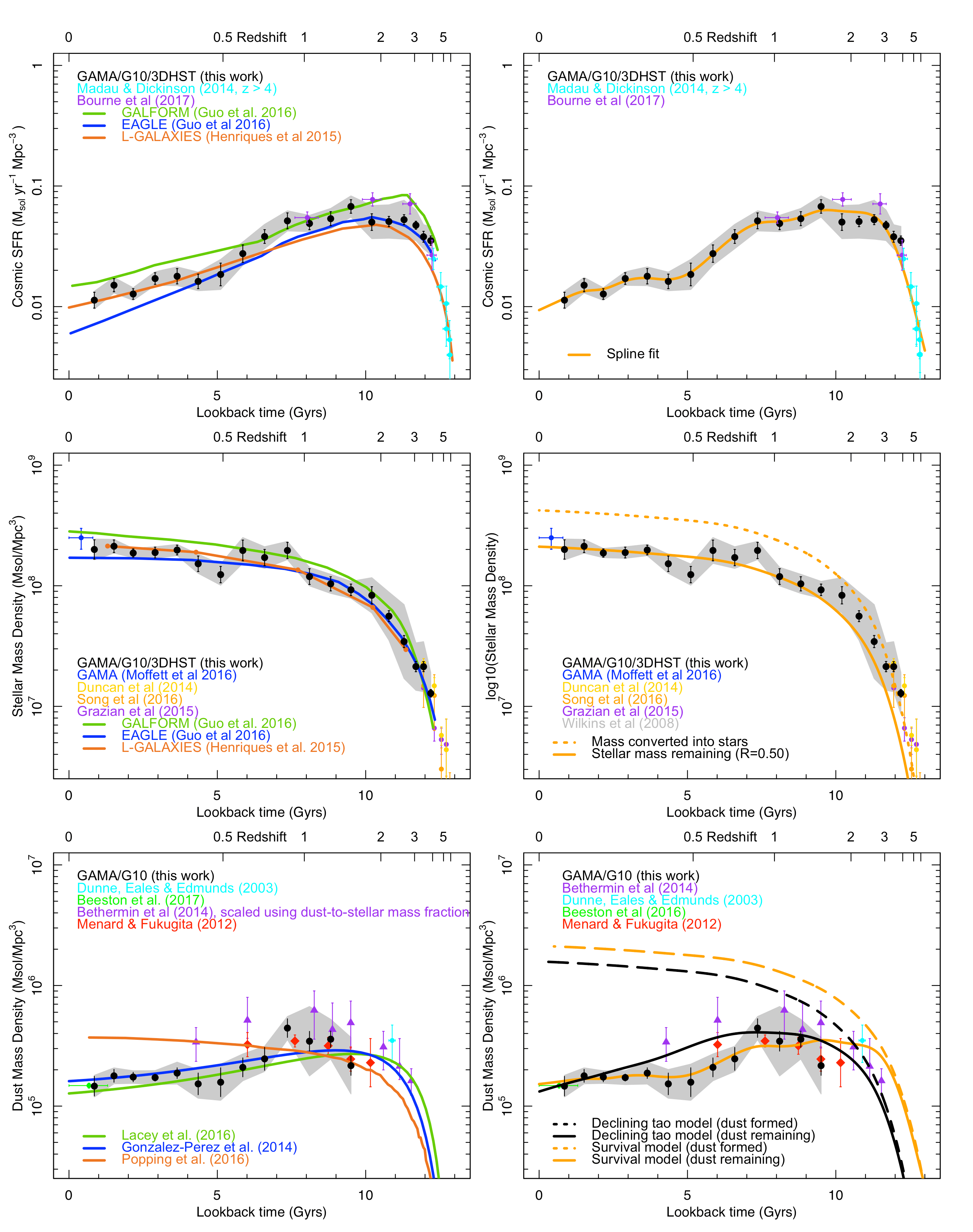
Figure 16: Our derived cosmic star-formation history (upper panels), stellar-mass build-up (middle panels) and dust mass build-up (lower panels) versus lookback time. Overlain are model lines as described in the text with predictions from numerical simulations (left-side panels), and our phenomenological model (right-side panels).

5 Discussion

The primary goal of this paper is to provide homogenous data of the cosmic star-formation history, the stellar mass density and dust mass density as shown in Figs. 13,14, & 15 and Tables 4, 5, &6. Here we briefly compare these data to the outputs of simulations, as well attempt to build a phenomenological model of the dust evolution, and complete by putting the new data into the context of the evolution of the baryon budget.

5.1 Comparison to numerical, hydro and semi-analytic simulations

Fig. 16 (left side panels) shows our results and selected data (for clarity), but now compared to various curves produced from semi-analytic or hydrodynamical models.

We show in Fig. 16 the CSFH adopted by GALFORM (Guo et al. 2016, which uses the Gonzalez-Peres et al. 2014 version of GALFORM; green line), EAGLE (Guo et al. 2016; mauve line), and L-GALAXIES (Henriques et al. 2015; orange line). We see that EAGLE tends to under-predict our CSFH at very late times but by relatively modest amounts. GALFORM, on the other-hand agrees very well at intermediate ages just slightly over-predicting the CSFH in the 1-5Gyr lookback time range. Also shown (orange line) is the latest version of the Munich semi-analytic model (L-GALAXIES) by Henriques et al. (2015). This includes the Henriques et al. (2013) prescription to re-incorporate gas ejected from SN feedback in order to delay star-formation in low mass galaxies, and avoid excessive build-up of these objects at early times. In addition, it implements a slight modified version of AGN radio model feedback, a lower star-formation threshold and ram-pressure stripping only in clusters. Combined, these modifications ensure that massive galaxies are predominately quenched at earlier times while low mass galaxies have star-formation histories more extended towards the local Universe. As can be seen this results in a slight under-prediction at very high-redshift, compared to our data, but a better fit locally.

Overlain on Fig. 16 (middle left side panel) are the same three models from the GALFORM (Guo et al. 2016), EAGLE (Guo et al. 2016), and L-GALAXIES (Henriques et al. 2015) simulations, compared to our measured evolution of the stellar mass density. Generally as for the CSFH, these mostly provide a good representation to the data with the GALFORM data slightly over-predicting the total stellar mass content at late times — inline with their enhanced late-time star-formation and EAGLE slightly under-predicts. Nevertheless the agreement between the models and data is noteworthy particularly as while the simulations are calibrated to the $z=0$ galaxy stellar mass function, they have not been tailored to reproduce the cosmic star-formation history or the stellar-mass build-up in detail.

Finally overlain on Fig 16 (lower left side panel) are two prescriptions from GALFORM for dust evolution (Lacey et al. 2016 and Gonzalez-Perez et al. 2014). The GALFORM models presented here have very different assumptions for the IMF. The Gonzalez-Perez et al. (2014) model assumes a universal MW-like IMF, while Lacey et al. (2016) introduced a top-heavier IMF during starbursts. The latter is done to allow for quick metal enrichment at high redshift in very star-forming galaxies, so that the model can reproduce the abundance and luminosities of dusty galaxies. Consequently, the Lacey et al. model predicts a larger dust abundance at higher redshift compared to the Gonzalez-Perez et al. model. Towards lower redshift this inverts due to the Lacey et al. model predicting lower gas fractions of galaxies than the Gonzalez-Perez et al. model (see Lagos et al. 2014 for a comparison of the cosmic gas density in these two models), and under the model assumption of a metallicity dependent dust-to-gas ratio, this directly translates into a lower dust abundance. Nevertheless both curves match the data reasonably well across the full redshift range despite the relatively sweeping assumptions adopted in the dust prescriptions.

A more dust-focused model by Popping et al. (2016), which advocates dust ejection, marginally under-predicts at early times and significantly over-predicts at later times. In their model dust is lost into the CGM and ejected, but is still forming dust faster than it is being ejected, resulting in an upward trend in the predicted dust density. Our measurements should include both the ISM and close-in CGM dust, but would miss fully ejected material. However more critical is the decline that we see which, as it derives mainly from the more massive systems, strongly supports the notion of dust destruction over ejection.

Overall the simulations seem to be doing pretty well in reproducing the cosmic star-formation history, the stellar mass build-up, and dust density evolution with the largest concern being, curiously, the redshift zero star-formation rates which are over or under predictions compared to our measurements for GALFORM and EAGLE respectively, by $\sim 50$ per cent. Conversely L-GALAXIES manage to match the very-high, intermediate, low-z Universe extremely well but just slightly under-predict our CSFH measurements at very early times (i.e., $2.5<z<4$).

We finish this section by advocating that the data presented here (Tables 4, 5, & 6), represents the first homogeneous sample of the CSFH, SMD and DMD over all time, and therefore optimal to inform (calibrate) future numerical, hydrodynamical, and semi-analytic simulations.

5.2 Phenomenological modelling

Fig. 16 (right side panels) essentially encodes the life-cycle of stars and dust and can ultimately be used to place hard empirical constraints on factors such as the mass-return fraction, stripped stellar mass, dust production rate and dust destruction rate. The key of course is the CSFH which provides an empirical-based description of the rate at which stars form. Explicitly under the assumption of a constant Chabrier IMF, the stellar-mass density can be represented by the cumulative distribution of the CSFH, modulo mass returned to the ISM and mass-lost through ejection, stripping or other processes. The orange line on Fig. 16 (right side panels) represents a simple spline-fit to our CSFH where we also include the Madau & Dickinson (2014) data with $z>4$ and the recent Bourne et al. (2017) data. The spline shows a good fit to all the data points. Integrating this spline-fit yields the cumulative stellar-mass density excluding mass-loss. This is shown as the dashed line in the middle right side panel of Fig. 16 and while fitting the data at very early lookback times clearly exceeds the measurements at latter times. The obvious explanation is replenishment of the ISM through stellar mass-loss, but one cannot rule out an additional portion arising due to stellar-mass also being stripped or ejected from the individual galaxies, i.e., that which ultimately makes up the intra cluster- and intra-group light.

Integrating the CSFH spline to z=0.0 we find a total mass converted into stars of $(4.2\pm 0.2)\times 10^{8}$M_⊙Mpc^-3 (at $z=0.0$) compared to our measured value (see Tables 4,5, & 6) of $(2.1\pm 0.4)\times 10^{8}$M_⊙Mpc^-3 (at $z\approx 0.1$). Correcting for the slight redshift offset this implies a mass-loss factor of $(0.50\pm 0.07)$. This is consistent with that expected for a Chabrier IMF (see Courteau et al. 2014, figure 3) of 0.44. This agreement is extremely good and suggests that the CSFH and stellar-mass density are in close agreement. It also leaves a little room for stripped or ejected stellar-mass, with implications for the optical ICL and IHL. Pushing to the limit of the error range suggests that $<13$ per cent of the stellar-mass is likely to be stripped, consistent with the $<20$ per cent value determined from EBL considerations (see Driver et al. 2016). One might also be tempted to use this as confirmation of the Chabrier IMF but the case is not entirely clear. Switching to an alternative IMF would result in both the CSFH and stellar-mass density varying in slightly different ways depending exactly how the stellar-masses were derived (i.e., via single band optical, near-IR, colours or full SED fitting). We can, however, say that the simplistic assumption of a universal Chabrier IMF is fully consistent with our homogenised measurements of the CSFH and stellar-mass density based on our MAGPHYS analysis. Adding in a mass-loss factor of 0.49 we can now re-plot the predicted stellar-mass as the solid black line (Fig. 16, middle right side panel) yielding a consistent fit throughout. The implication being $44$ per cent of this is through normal stellar mass loss processes, and $6\pm 7$ per cent through stripping via merging and/or harassment.

Moving to Fig. 16 (lower right side panel) we see the dust mass density evolution which represents relatively new territory. The recent study by Popping, Somerville & Galametz (2016) argued that dust is rapidly formed with minimal destruction and continuously accumulates with some portion ejected into the CGM and beyond. Our data, following on from Dunne et al. (2011), disagrees as we see a gradually declining dust density from early times to the present day. While we cannot rule out a systematic upward error in our dust measurements towards higher-z, particularly as we rely more heavily on optical/near-IR data combined with upper-limit estimates, our data also appear to agree reasonable well with literature constraints. At low redshift the data of Dunne et al. (2003, 2011), Vlahakis et al. (2005) appear fully consistent, as do the data based on MgII absorbers from Menard & Fukugita (2012). In comparison to the Bethermin data, rescaled using a constant dust to stellar mass ratio, we do see some discrepancy but this does include the adoption of a universal dust-to-stellar mass ratio.

Given that we see a steady decline in the dust mass density, dust destruction is clearly critical. This is non-controversial given the known lack of dust in old massive Elliptical systems where ejection processes are unlikely to be effective (because of the halos ability to retain ejected mass). We therefore consider two simplistic toy models. One where the dust is destroyed globally (by assigning some dust half-life), and one where it is destroyed locally (by assigning some survival fraction). The toy models are intended to convey the notion that in the first scenario

dust is formed and escapes the star-forming region but ultimately depleted through astration or expulsion from the galaxy by either radiation pressure or galactic winds. The second assumes that while dust is formed in star-forming regions, the majority of it might also be destroyed in the same location by supernova shocks. Most likely both processes are occurring but it is convenient to ask if both scenarioes are independently viable.

For the declining tao model we can introduce the idea of dust destruction via a simple exponential decay:

$$\mbox{i.e.,}M_{D}(t_{z})=\sum_{t=0}^{t=tz}\epsilon\psi_{*}(t)e^{-\frac{t_{z}-t}{\tau}}$$ (1)

where $\epsilon$ is the fraction of dust formed per unit stellar mass, $\psi_{*}$ is the cosmic star-formation rate at time $t$, $\tau$ is the dust-folding time and $M_{D}(t_{z})$ is the dust mass remaining at time $t_{z}$. A simple match to the literature data (red and mauve points), then provides best fit parameters of:

$\epsilon$ = $0.004^{+0.001}_{-0.001}$

$\tau$ = $2.25^{+0.5}_{-0.5}$ Gyr

Note that we fit the literature data, as this simple model struggles to match the shape of our data at around 5Gyr look back time where there is an obvious dip (which we assume is due to CV). The arbitrary fitting function we have adopted, and shown by the solid black line on Fig. 16 (lower left), appears to trace the literature data very well. At face value this function suggests that dust destruction (or loss), is indeed a major factor, and while a significant amount of dust is formed the majority is either destroyed (i.e., via astration), or lost (i.e., ejected).

In our second model we adopt a constant dust survival fraction, i.e., a constant fraction of dust is formed during star-formation, the majority of which is destroyed in situ. This model is shown by the orange line and follows our data (rather than the literature data), extremely closely. Here we have adopted a formation rate of 0.0065 dust masses for every unit of stellar mass formed of which 5 per cent survives indefinitely.

Note that the dotted black and orange lines show the cumulative dust formation curves (i.e., ignoring the dust destruction mechanism). While the two scenarioes are quite different they plausibly bracket the extreme scenarioes where dust is destroyed globally (the declining tau model) or locally (the constant survival model). This essentially informs us that the full set of models that incorporate both global and local mechanisms are also likely to be plausible. Finally we note that of course the dust formation fraction may also evolve with time as the ambient ISM metallicity increases. Exploring these various effects will clearly require additional data and constraints and we leave this for further future work.

However, it is interesting (or perhaps obvious) that the two toy models, despite their differences, both predict similar fractions for the total dust mass formed. From our two toy models we can now infer that at $z=0$ the total amount of dust formed is $(2.1$—$1.6)\times 10^{6}$M_⊙Mpc^-3, yet we measure a density of $(1.5\pm 0.2)\times 10^{5}$M_⊙Mpc^-3, implying that approximately 90 to 95 per cent of all dust formed has either been destroyed (most likely), or ejected into the IGM (less likely given our measurements are mostly constrained by massive systems with strong gravitational fields).

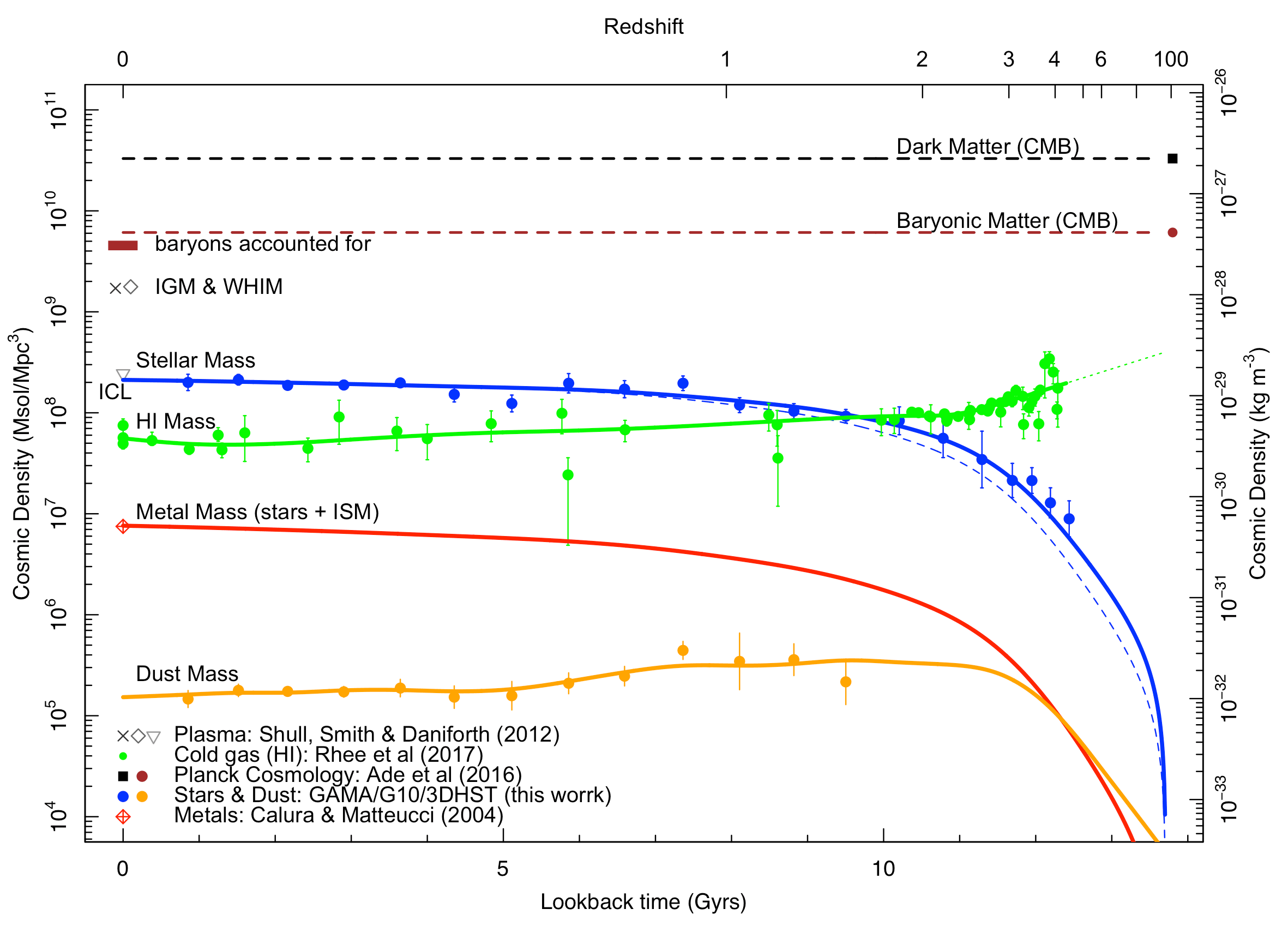
Figure 17: Our findings placed in the context of the mass budget and its evolution since the Big Bang.

5.3 Implications for the bound baryon budget and its evolution over time

We return now to the opening discussion on the evolution of the baryons and present an overview perspective in Fig. 17. This includes the base measurements of the dark matter density and baryon density from CMB studies (Ade et al. 2016) as well as the IGM, WHIM and ICL values reported in Shull, Smith & Danforth (2012). Now we can add the stellar mass and dust mass density derived here (blue and orange points respectively). We can also provide a simple estimate of the metal evolution by adopting a fixed yield and tying metal production to the total mass going into star-formation. This we calibrate at $z=0$ by adopting the value for the mean metallicity in the present day Universe from Calura & Matteucci (2005). Finally we include the cosmic HI compendium from Rhee et al. (2017) shown as green data. The figure paints an interesting picture, not least of which is how the almost mirror image between the stellar mass and cosmic HI mass trends. The simplest interpretation is that the sum of stars and HI is constant, i.e., gas is imply turned into stars and not replenished. However we note the very large errors associated with the HI measurements and the need for further measurements in the intermediate age range.

6 Summary

We have combined data from the GAMA, G10-COSMOS, and 3D-HST surveys to produce a meta-catalogue which samples the stellar-mass, dust-mass and star-formation measurements over a broad mass/star-formation range and over all time. For the GAMA, G10-COSMOS and 3D-HST datasets we use the popular energy-balance code MAGPHYS to determine cosmic star-formation rates, stellar-mass, and dust-mass densities. These values compare well with previous estimates and now constitute a homogenous set of measurements across the full timeline of the Universe.

We construct histograms of the star-formation, stellar-mass, and dust-mass space-densities and their associated first moments which represent their differential contribution to the overall mass and star-formation budgets. After identifying appropriate limits for each dataset we use a 7-point spline to simultaneously fit all three datasets weighting by the inverse errors squared. In general the three datasets show good agreement and the spline fits are well behaved allowing us to determine the cosmic star-formation rate, stellar-mass and dust-mass densities reliably over a consistent mass and star-formation range and over a broad range in redshift.

The resulting cosmic star-formation density, stellar-mass density, and dust-mass density versus lookback time agree reasonably well with previous estimates but constitute a major advancement in terms of homogeneity, and sample-size. In particular at intermediate lookback times the combination of GAMA with G10-COSMOS and 3D-HST enables robust sampling of the full dynamic range of masses and star-formation rates with GAMA defining the high mass, high star-formation rate end with high significance and G10-COSMOS defining the low mass/star-formation rate end. As a consequence the scatter implied by our measurement is a significant advancement over the previous compendium of disparate datasets. In particular the stellar-mass density and star-formation densities are now known over a 12 Gyr period with an uncertainty at any time interval of $<\sim\pm 30$ per cent. The data are provided in Tables 4, 5, & 6.

Our measurement of the dust mass density over lookback time represents the first tentative study of dust over such a broad range of time and builds on the earlier HAtlas-SDP study of Dunne et al. (2011). While our data formally agree over the lookback range in common within the quoted errors we do not agree with the conclusion of a rapid declining dust mass density. Instead we find a steady but shallower decline in the dust density from a peak somewhere between 7 — 10 Gyrs ago. We note that the hydro and semi-analytic models tested here also reproduce reasonably well the cosmic star-formation history, the stellar-mass dust build-up, and the evolution in the dust mass density.

We attempt to explore consistency across the three density distributions. Starting with a spline-fit to our cosmic star-formation history we find that we predict the stellar mass density at later times in agreement with the findings of Madau & Dickinson (2014) recovering a stellar-mass replenishment factor of ($0.50\pm 0.07$), consistent with our adopted Chabrier IMF and some addition stellar-mass loss through stripping ($0.06\pm 0.07$).

Again starting from our CSFH spline-fit we show two simple toy models where dust formation is closely linked to the cosmic star-formation history and dust destruction follows either an exponential decline or a constant survival fraction. From our models, that bracket the range of data, we conclude that for every unit of stellar mass that is formed 0.0065 — 0.0040 units of dust mass is formed and that over the lifetime of the Universe approximately 90 — 95 per cent of all dust which has formed is unaccounted for: either it is destroyed, ejected or a combination of both.

Finally we show how our results mesh with the unfolding picture of the evolution of the bound baryons from the early Universe to the present day with the rise in stellar mass appearing to mirror the evolution of the cosmic HI density, but with low significance due to the inherent uncertainties.

This work is a preliminary step which demonstrates the power of linking comprehensive high quality datasets which each sample distinct regions of the mass-redshift plane. Obvious improvements to this work include improved measurements of far-IR fluxes, particularly for the G10-COSMOS and the 3D-HST fields, both through improved analysis but also improved observations such as might become available through the proposed future NASA Origins mission.

References

Planck Collaboration: Ade P.A.R. et al. 2016, A&A, 594, 13

Ahn C.P., et al., 2014, ApJS, 211, 17

Andrews S.K., Driver S.P., Davies L.J.M., Kafle P.R., Robotham A.S.G., Wright A.H., 2017a, MNRAS, 464, 1579

Andrews S.K., et al., 2017b, MNRAS, in press

Andrews S.K., et al., 2017c, MNRAS, submitted

Baldry I.K., Glazebrook K., 2003, ApJ, 593, 258

Baldry I.K., Glazebrook & Driver, 2008, MNRAS, 388, 945

Baldry I.K., et al., 2010, MNRAS, 404, 86

Baldry I.K., et al., 2012, MNRAS, 412, 621

Baldry I.K., et al., 2014, MNRAS, 441, 2440

Béthermin M., et al., 2014, MNRAS, 567, 103

Beeston R., et al., 2017, MNRAS, in prep.

Bertin E., 2011, ASPC, 442, 435

Bonamente M., Nevalainen J.M., Tilton E., Liivamäge, Tempel E., Heinämäki, Fang T., MNRAS, 457, 4236

Bondi M., Ciliegi P., Schinnerer R., Smolcic V., Jahnke K., Carilli C., Zamorani G., et al., 2008, ApJ, 681, 1129

Bourne N., et al. 2016, MNRAS, 462, 1714

Bourne N., et al. 2017, MNRAS, in press (arXiv:1607.04283)

Bouwens R.J., et al. 2012a, ApJ, 752, 5

Bouwens R.J., et al. 2012b, ApJ, 754, 83

Burgarella D., et al., 2013, A&A, 554, 70

Brammer G., et al., 2012, ApJ, 758, 17

Calura F., Matteucci F., 2004, MNRAS, 350, 351

Capak P., et al., 2007, ApJS, 172, 99

Chabrier G., 2003, PASP, 115, 763

Clemens M.S., et al., 2013, MNRAS, 433, 695

Colless M., et al., 2001, MNRAS, 328, 1039

Courteau, S et a., 2014, RvMP, 86, 47

Cool R.J., et al., 2013, ApJ, 767, 118

Cucciati O., et al., 2012, A&A, 539, 31

Cyburt R.H., Fields B.D., Olive K.A., Yeh T-H., 2016, 88, 5004

da Cunha E., Charlot S., Elbaz, D., 2008, MNRAS, 388, 1595

Danforth C.W., et al., 2016, ApJ, 817, 111

Dariush A., et al., 2016, MNRAS, 456, 2221

Davies L.J.M., Driver S.P., Robotham A.S.G., Baldry I.K., Lange R., Liske J., Meyer M., Popping A., Wilkins S.M., Wright A.H., 2015, MNRAS, 447, 1014

Davies L.J.M., et al., 2016, MNRAS, 461, 458

Decarli R., et al., 2016, ApJ, 833, 69

Delhaize J., Meyer M.J., Staveley-Smith L., Boyle B.J., 2013, MNRAS, 433, 1398

Donley J.L., et al., 2012, ApJ, 748, 142

Driver S.P., Robotham A.S.G., 2010, MNRAS, 407, 2131

Driver S.P., et al., 2009, A&G, 50, 12

Driver S.P., Popescu C.C., Tuffs R., Liske J., Graham A.W., Allen P.D., de Propris R., 2007, MNRAS, 379, 1022

Driver S.P., et al., 2012, MNRAS, 427, 3244

Driver S.P., et al., 2011, MNRAS, 413, 971

Driver S.P., et al., 2016, ApJ, 827, 108

Duncan et al, 2014, MNRAS, 444, 2960

Dunne, L., Eales, S.A., Edmunds M.G., 2003, MNRAS¡ 341, 589

Eales S., et al., 2010, PASP, 122, 499

Eckert D., et al., 2015, Nature, 528, 105

Fukugita, Hogan & Peebles, 1998, ApJ, 503, 518

Gall C., Hjorth J., Watson D., Dwek E., Manaund J.R., Fox, O., Leloudas G., Malesani D., Day-Jones A.C., 2014, Nature, 511, 326

Gonzalez-Perez V., Lacey C.G., Baugh C.M., Helly C.D.P., Campbell D.J.R., Mitchell P.D., 2014, MNRAS, 439, 264

Graham A., Driver S.P., Allen P.D., Liske J., 2007, MNRAS, 378, 198

Grazian A., et al., 2015, A&A, 575, 96

Grootes M., et al., 2013, ApJ, 766, 59

Grootes M., et al., 2016, MNRAS, submitted

Guo Q., et al, 2016, MNRAS, 461, 3457

Gunawardhana M., et al., 2013, MNRAS, 433, 2764

Gunawardhana M., et al., 2011, MNRAS, 415, 1647

Hayward C.C., Smith D.J.B., 2015, MNRAS, 446, 1512

Henriques B., White S.D.M., Thomas P.A., Angulo R.E., Guo Q., Lemson G., Springer V., 2013, MNRAS, 431, 3373

Henriques B., White S.D.M., Thomas P.A., Angulo R., Guo Q., Lemson G., Springel V., Overzier R., 2015, MNRAS, 451, 2663

Hernandez-Monteagudo C., Ma, Y-Z., Kitaura F.S., Wang, W., Genova-Santos R., Macias-Perez J, Herranz, D., 2015, PhRvL, 115, 1301

Hinshaw G.F., et al., 2013, ApJS, 208, 19

Holwerda B., Dalcanton J.J., Radburn-Smith D., de Jong R.S., Guhathakurta P., Koekemoer A., Allen R.J., Böker T., 2012, ApJ, 753, 25

Hopkins A.M., Beacom J.F., 2006, ApJ, 651, 142

Hopkins A.M., et al., 2013, MNRAS, 430, 2047

Hurley P.D., et al., 2016, MNRAS, in press (arXiv:1606.05770)

Keres D., Yun M.S., Young J.S., 2003, ApJ, 582, 659

Kriek M., et al., 2009. 2009, ApJ, 700, 221

Kroupa P., 2001, MNRAS, 322, 231

Lagos C., Baugh C.M., Lacey C.G., Benson A.J., Kim H-S., Power C., 2011, MNRAS, 418, 1649

Lacey C., et al., 2016, MNRAS, 462, 3854

Laigle C., et al., 2016, ApJS, 224, 24

Le Fevre O., et al., 2013, A&A, 559, 14

Lilly S.J., Le Fevre O., Hammer F., Crampton D., 1996, ApJ, 460, 1

Liske J., et al., 2015, MNRAS, 452, 2087

Madau P., Dickinson M., 2014, ARA&A, 52, 415

Martin A.M., Papastergis E., Giovanelli R., Haynes M.P., Springob C.M., Stierwalt S., 2010, ApJ, 723, 1359

Martin C., et al. 2005, ApJ, 619, 1

Menard B., Fukugita M., 2012, ApJ, 754, 116

Moffett A., et al., 2016, MNRAS, 462, 4336

Momcheva I., et al., 2016, ApJS, 225, 27

Mutlu Pakdil M., Seigar M.S., David B.L., 2016, in press (arXiv:1607.07325)

Oliver S., et al., 2012, MNRAS, 424, 1614

Peng Y., et al., 2010, ApJ, 721, 193

Popping G., Somerville R.S., Galametz M., 2016, MNRAS, submitted (arXiv:1609.08622)

Rhee, J., et al., 2017, MNRAS, in press

Robotham A.S.G., Driver S.P., 2011, MNRAS, 413, 2570

Rowlands K., Gomez H.L., Dunne L., Aragon-Salamanca A., Dye S., Maddox S., da Cunha E., van der Werf P., 2014, MNRAS, 441, 1040

Sargent B., et al., 2010, ApJ, 878

Schenker M.A., et al., 2012, ApJ, 744, 179

Schinnerer R., et al., 2007, ApJS, 172, 46

Scoville N., et al., 2007a, ApJS, 172, 1

Scoville N., et al., 2007b, ApJS, 172, 38

Seymour N., et al., 2008, MNRAS, 386, 1695

Shankar F., Salucci P., Granato G.L., De Zotti G., Danese L., 2004, MNRAS, 354, 1020

Skelton R.E., et al., 2014, ApJS, 214, 24

Shull J.M., Smith B.D., Danforth C.W., 2015, ApJ, 811, 3

Smith D.J.B., et al., 2012, MNRAS, 427, 703

Song M., et al., 2016, ApJ, 825, 5

Stocke J.T. et al., 2013, ApJ, 763, 148

Sutherland W.J., 2015, A&A, 575, 25

Taniguchi Y., et al., 2007, ApJS, 172, 9

Valinate E., et al., 2016, MNRAS, 462, 3146

van Dokkum P., et al., 2013, ApJ, submitted (arXiv:13052140)

Vlahakis C., Dunne L., Eales D., 2005, MNRAS, 364, 1253

Vika, M., Driver S.P., Graham A.W., Liske J., 2009, MNRAS, 400, 1451

Walter F., et al., 2014, ApJ, 782, 79

Weingartner J.C., Draine B.T., 2001, ApJS, 134, 263

Whitaker K.E., 2014, ApJ, 795, 104

Wilkins S.M., Trentham N., Hopkins A.M., 2008, MNRAS, 385, 687

Wright A.H., et al., 2016, MNRAS, 460, 765

Wright A.H., et al., 2017a, MNRAS, submitted

Wright A.H., et al., 2017b, MNRAS, in prep

Wright E.L., et al., 2010, AJ, 140, 1868

York D., et al., AJ, 2000, 120, 1579

Zwaan M., Meyer M.J., Staveley-Smith L., Webster R.L., 2005, MNRAS, 359, 30

Appendix A Expanding the G10-COSMOS far-IR sampling

The original G10-COSMOS catalogue described in Andrews et al. (2016) used a fairly aggressive cascade in the far-IR to pre-determine which objects should be measured. Essentially an attempt to measure a flux using the LAMBDAR code was only made for a small fraction of the objects. This is because of the much lower comparative signal-to-noise of the HerMES PACS and SPIRE data as compared to the very deep Subaru data. In earlier attempts to measure all 170,000 systems from the HerMES data we found that the density of faint objects led to numerous instances of overlapping apertures (in fact every pixel has on average 10 overlapping apertures). The net result is that flux sharing codes such as LAMBDAR, when confronted with very poor resolution data and multiple targets within a single pixel, end up averaging the flux across all the objects and eroding the bright systems by redistributing their flux to the fainter objects. While LAMBDAR has a process to mitigate this, like any code, it has limits and when flooded with an excessive number of faint objects in very poor resolution data LAMBDAR simply fails. The way this was addressed in Andrews et al. (and also with XID+ in Hurley et al. 2016) is to introduce a prior via a cascade process, whereby only objects with likely measurable fluxes were measured. In Andrews et al. this was implemented via a cascade process whereas only objects with clear MIPS24$\mu$m data were passed forward for measurement. Those objects which had solid detections in PACS 100 $\mu$m or 160 $\mu$m were then passed on for SPIRE250 $\mu$m measurements and only those with detections in SPIRE250 $\mu$m passed on for SPIRE350 measurements etc. The net result is that of the initial 170,000 objects in the full G10-COSMOS i-band selected catalogue only 11925 had attempted measurements in MIPS24, PACS100 and PACS160 bands reducing to 7178, 3446 and 2636 in the SPIRE bands. Hence ultimately measurements were only attempted for 1.55 per cent of the original input catalogue. In review we believe this cascade was overly aggressive and in our first pass MAGPHYS catalogue many systems were found with predicted dust masses which should be detectable. We therefore decided to revisit the inputs to our LAMBDAR analysis and remeasure PACS and SPIRE fluxes for all objects with an initial $\log_{10}[\frac{M_{d}}{d_{l}^{2}}]>0.0,0.35$ or $0.5$ resulting in samples of the dustiest 24k, 12k or 6k objects. We ran all three catalogues through our LAMBDAR code on the PACS and SPIRE PEPS and HerMES data and reviewed the outputs. Comparing the output aperture masks to the input image we established that the 24k catalogue was appropriate for PACS and SPIRE 250, the 12k catalogue appropriate for SPIRE 350 and the 6k catalogue appropriate for SPIRE500. These revised output catalogues were then spliced into G10CosmosLAMBDARCatv05 (Andrews et al. 2016) to make G10CosmosLAMBDARCatv06 which was used in this work.

Appendix B Extended analysis plots

Figs 18 to B18 show the analysis fits in all redshift bands for the cosmic star-formation (upper panels), stellar mass (middle panels), and dust mass (lower panels) distributions.

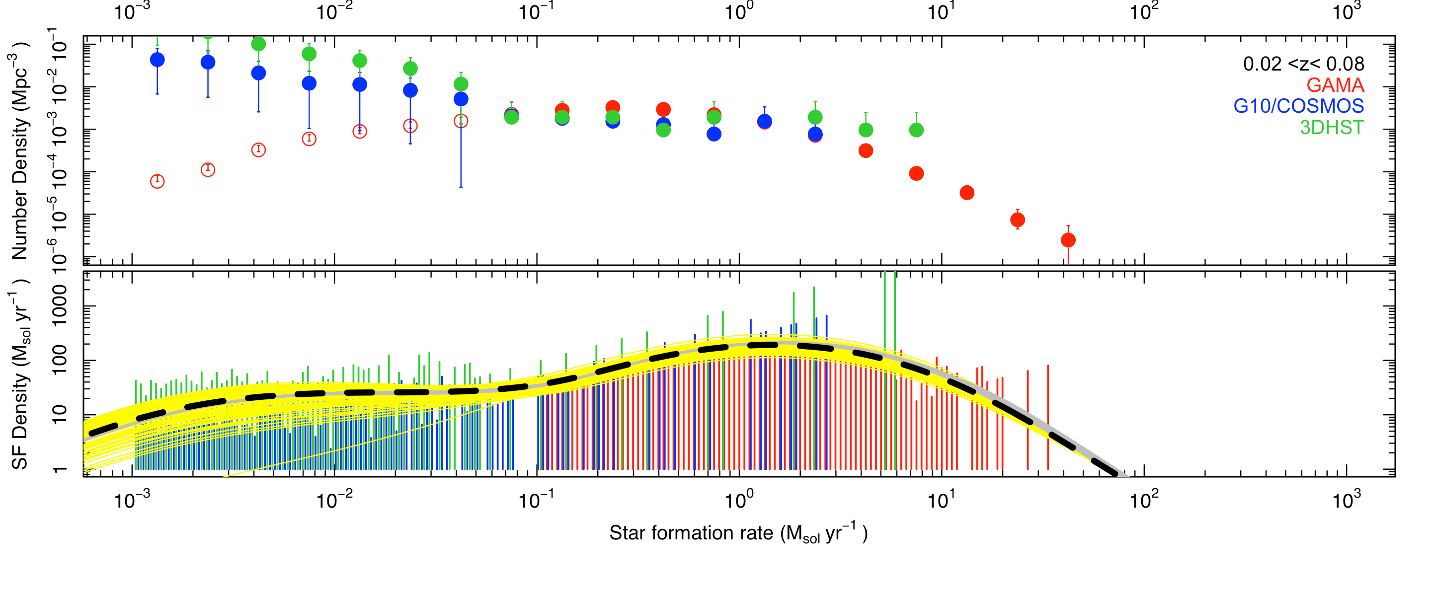
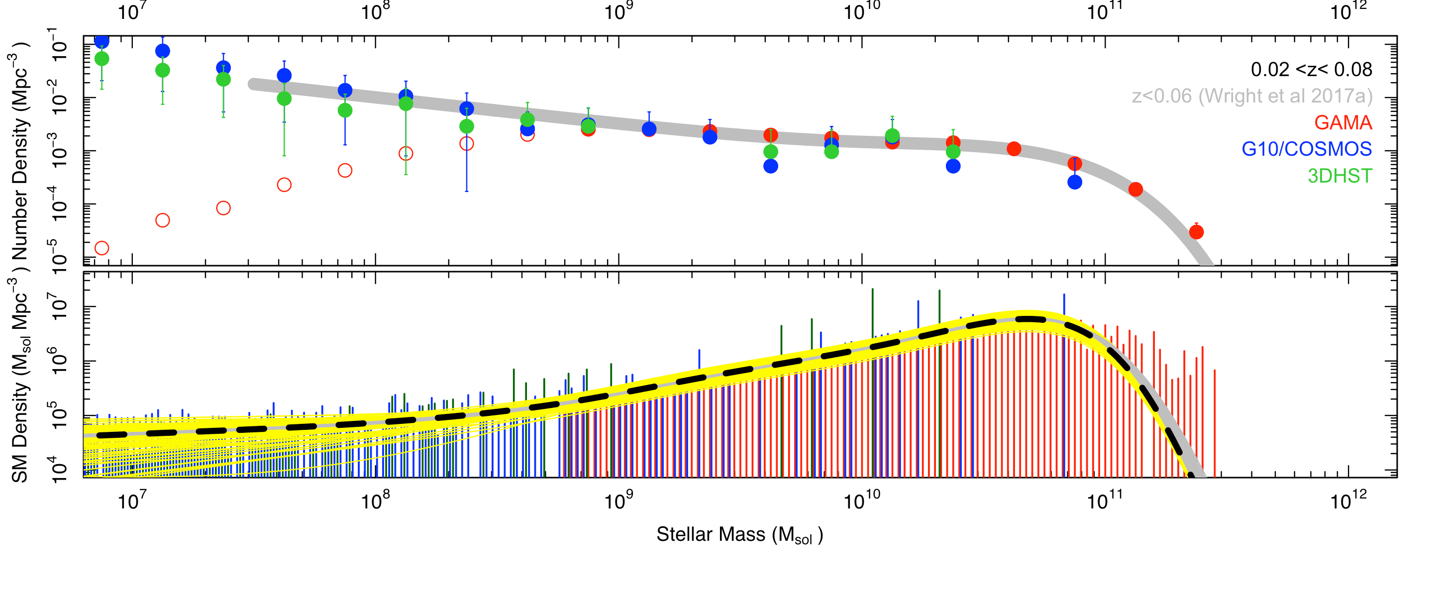
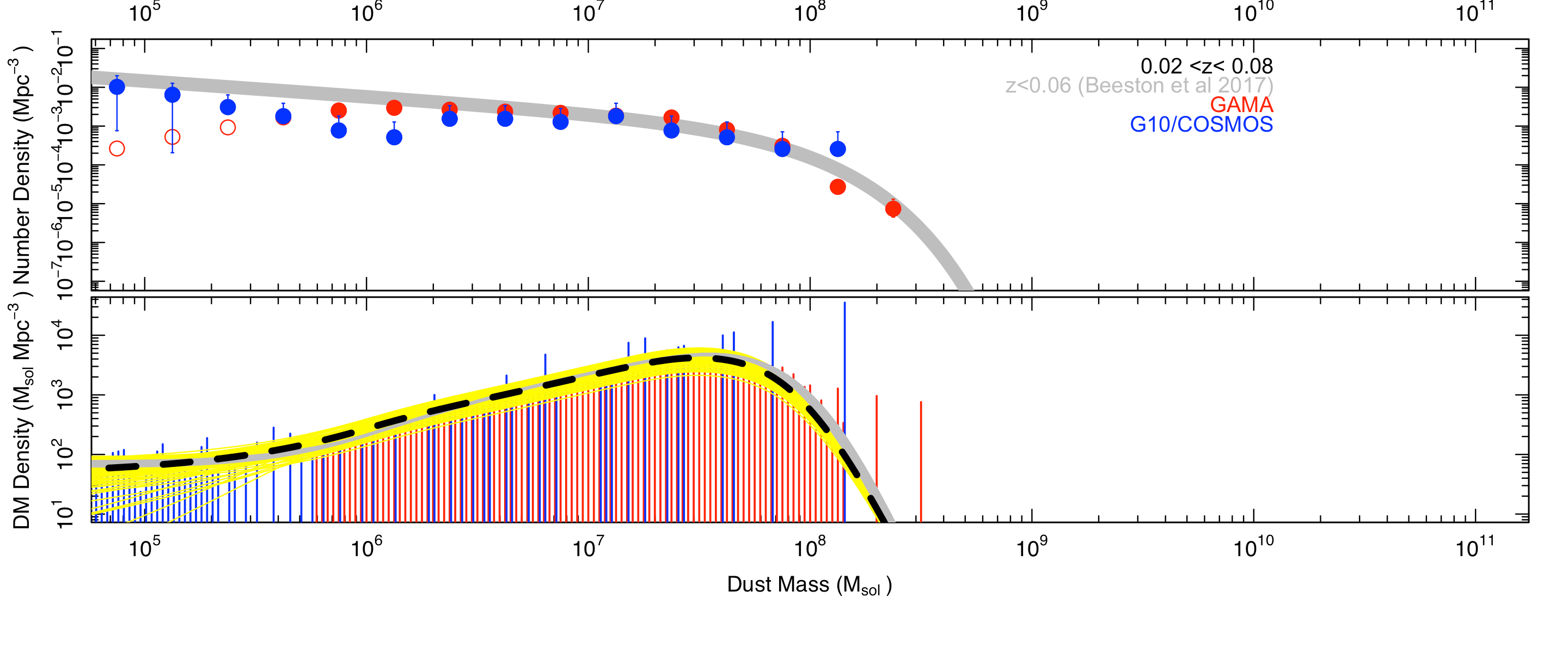
Figure 18: As for Fig. 12 except for the redshift range indicated.

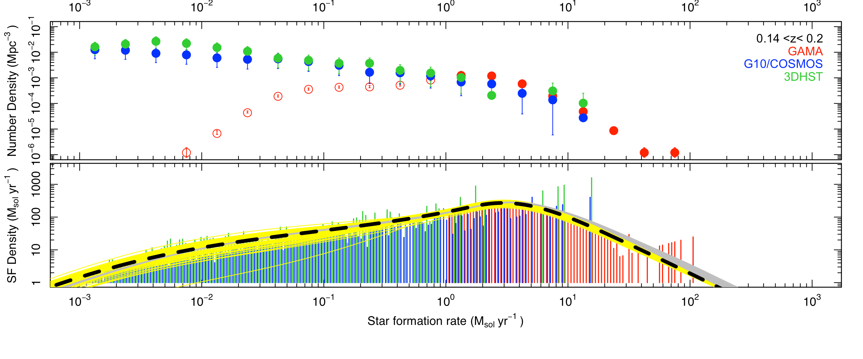
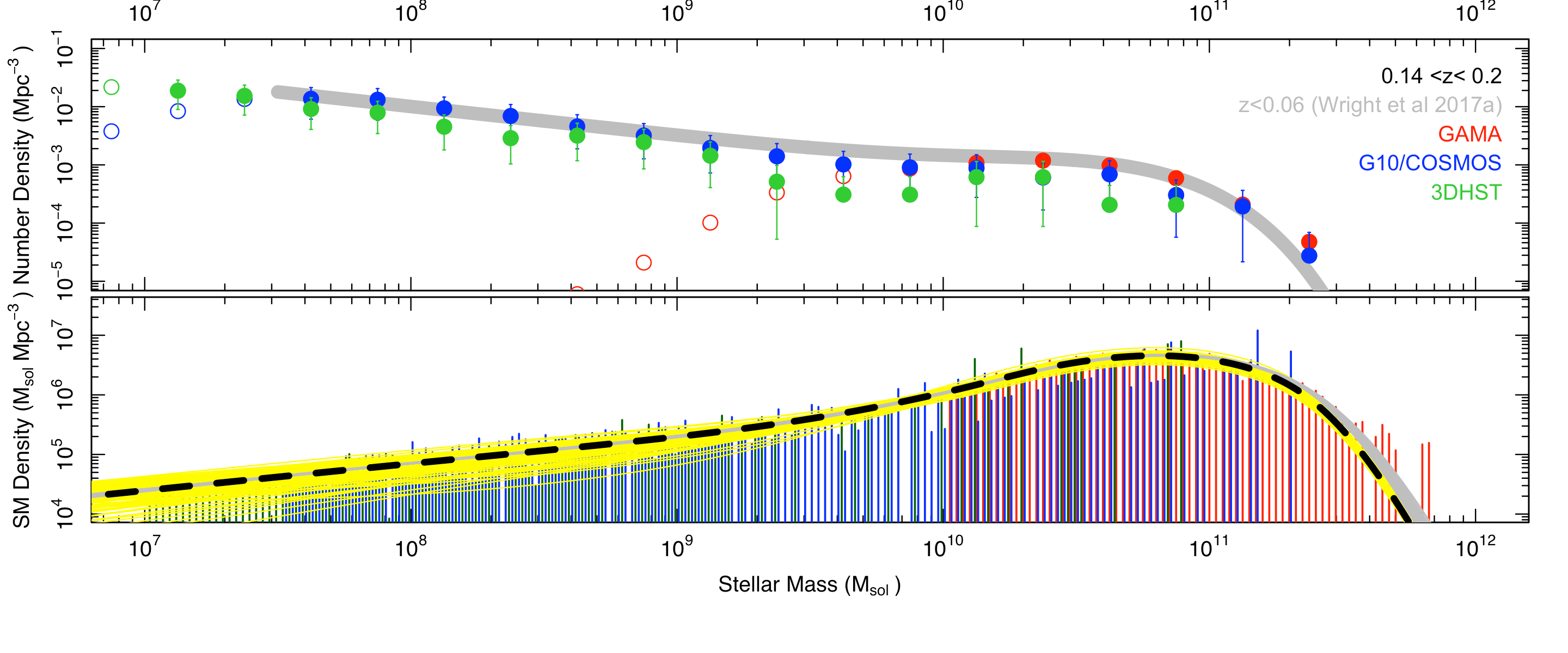
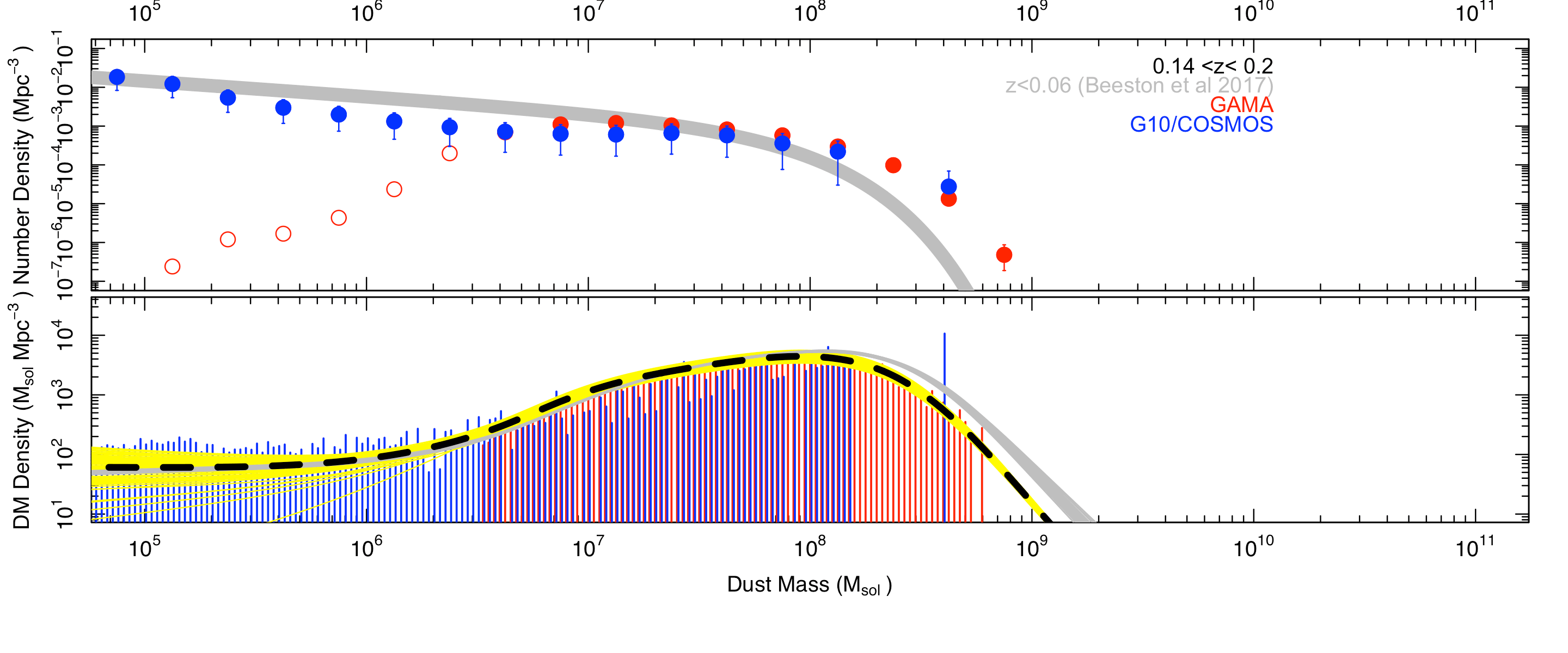
Figure 19: As for Fig. 12 except for the redshift range indicated.

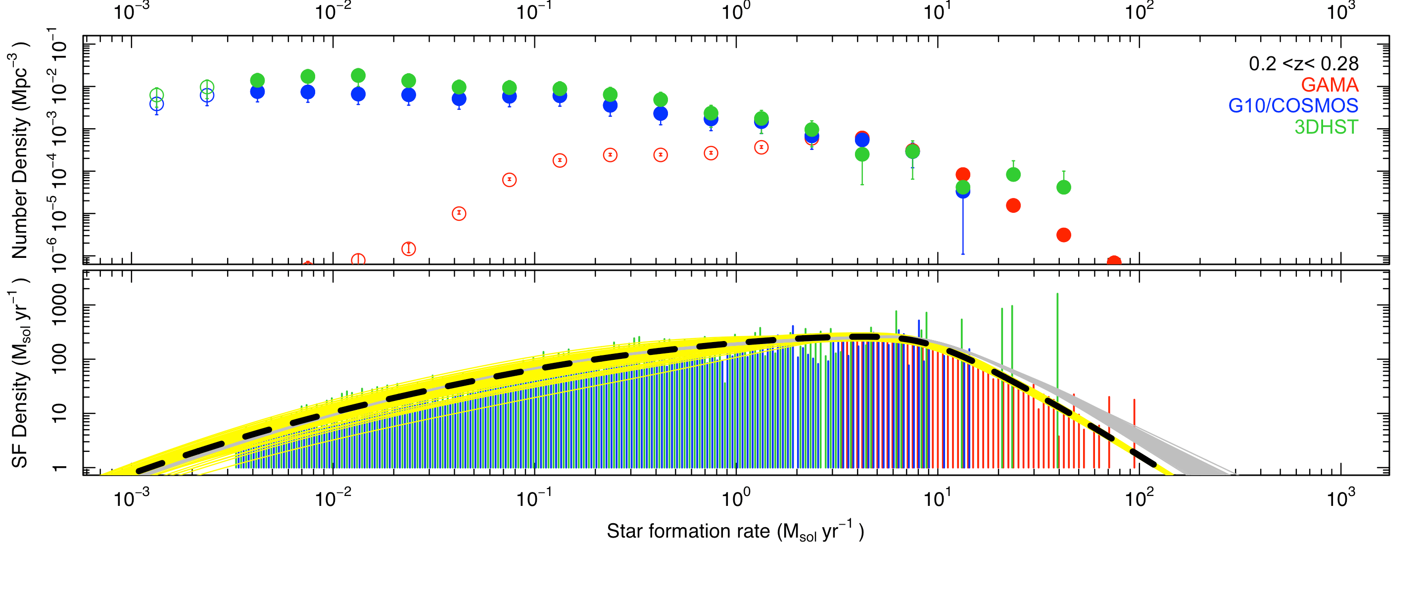
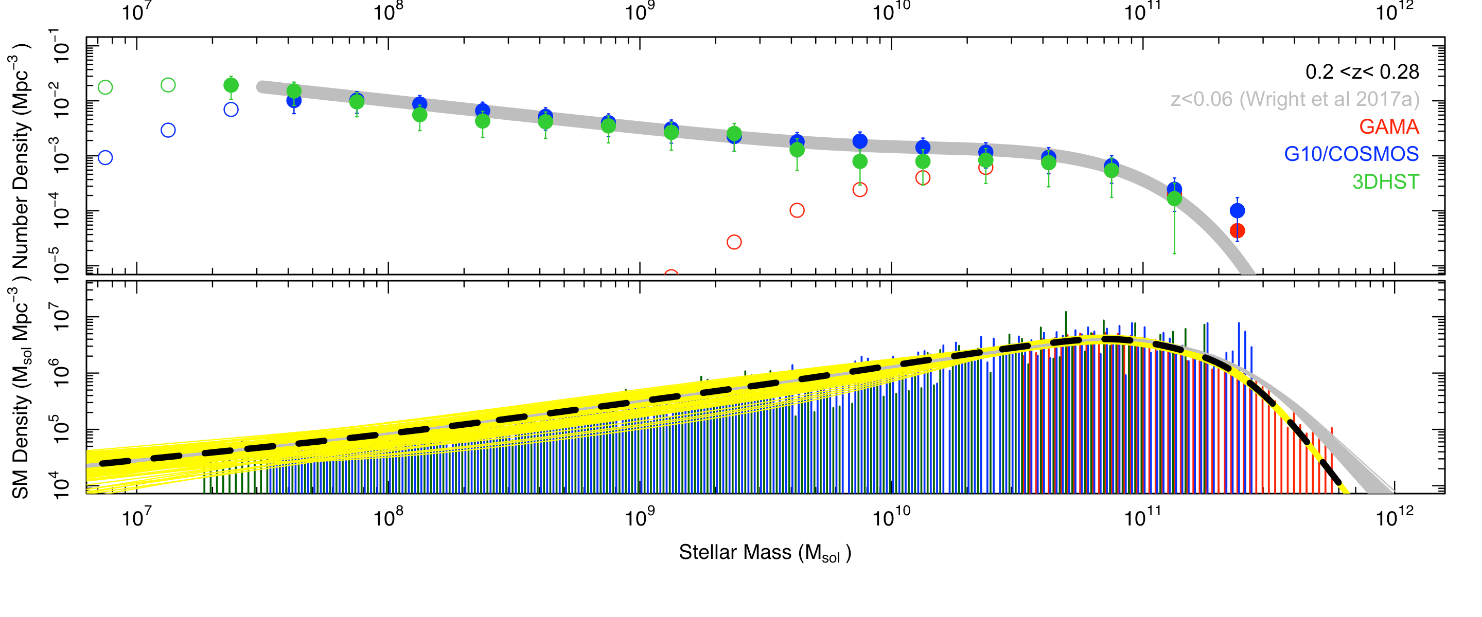
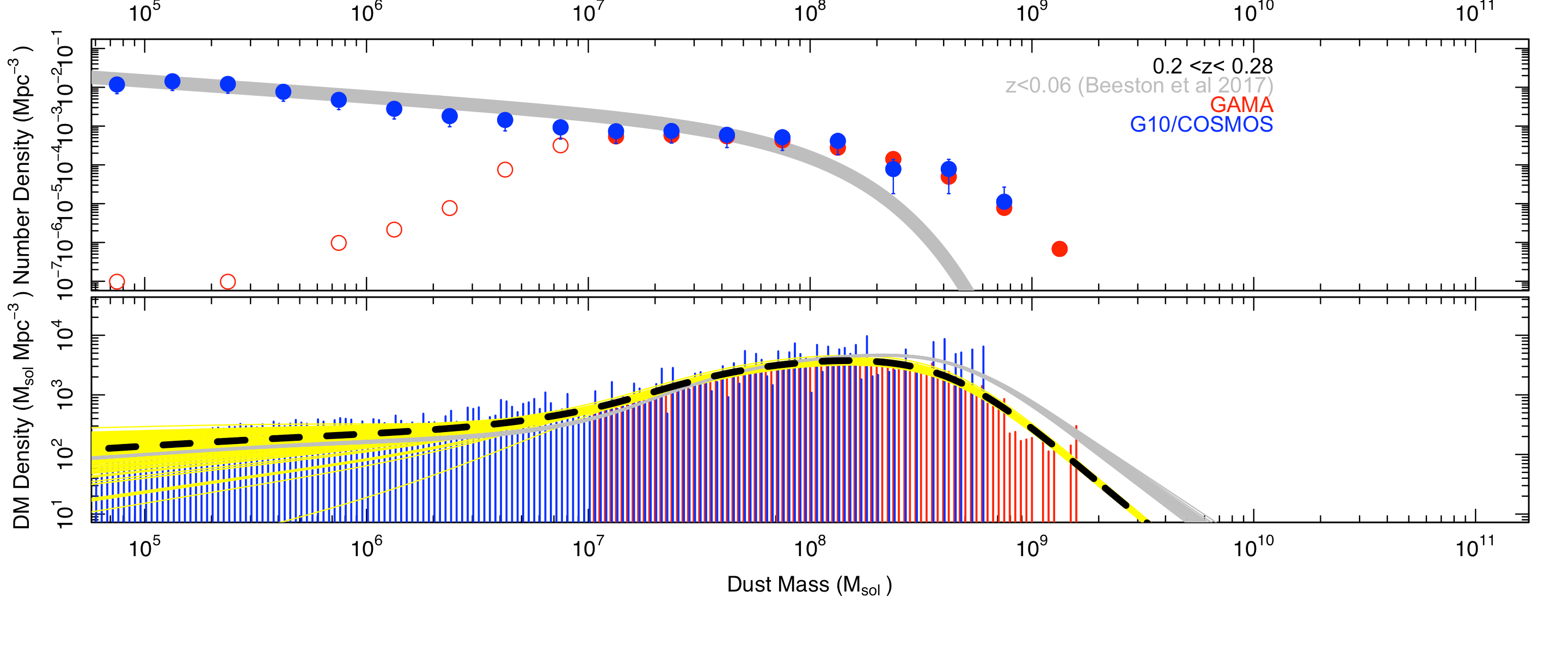
Figure 20: As for Fig. 12 except for the redshift range indicated.

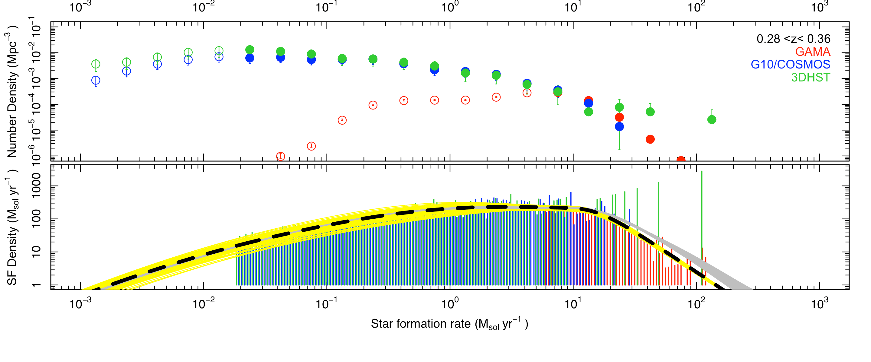
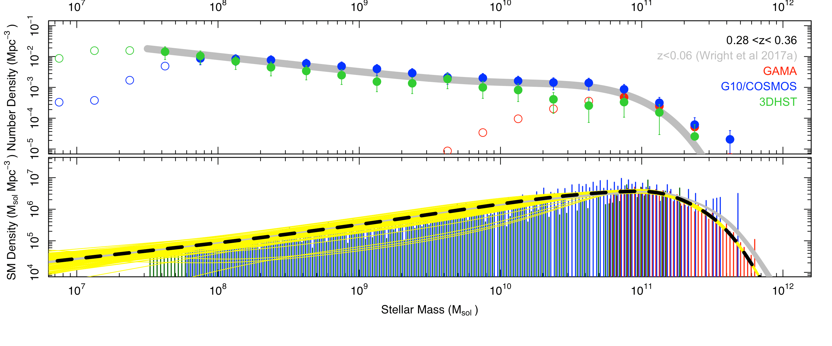
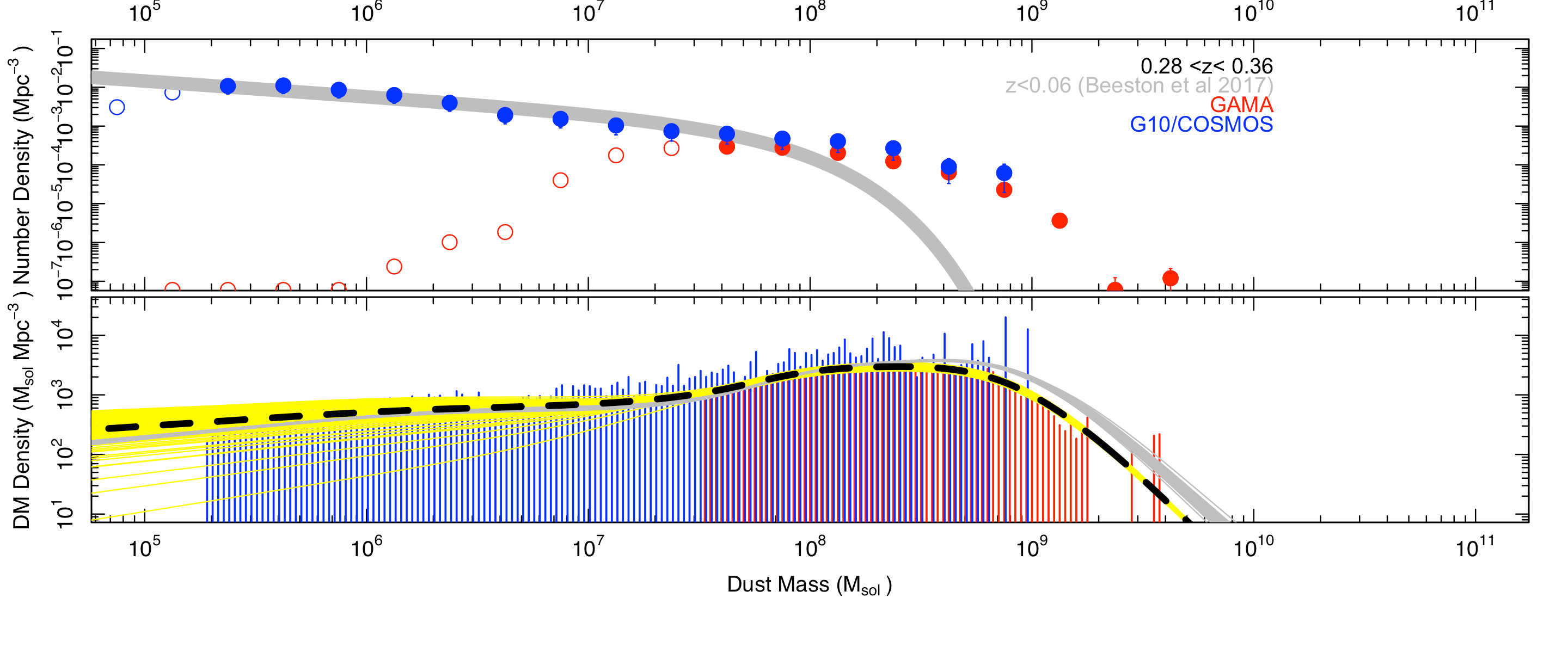
Figure 21: As for Fig. 12 except for the redshift range indicated.

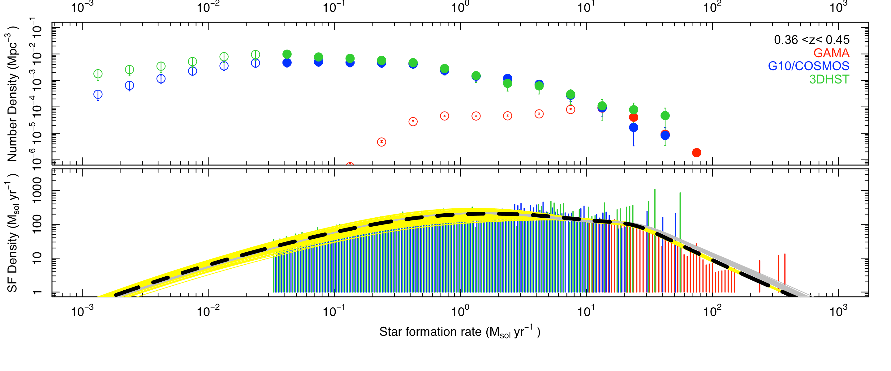
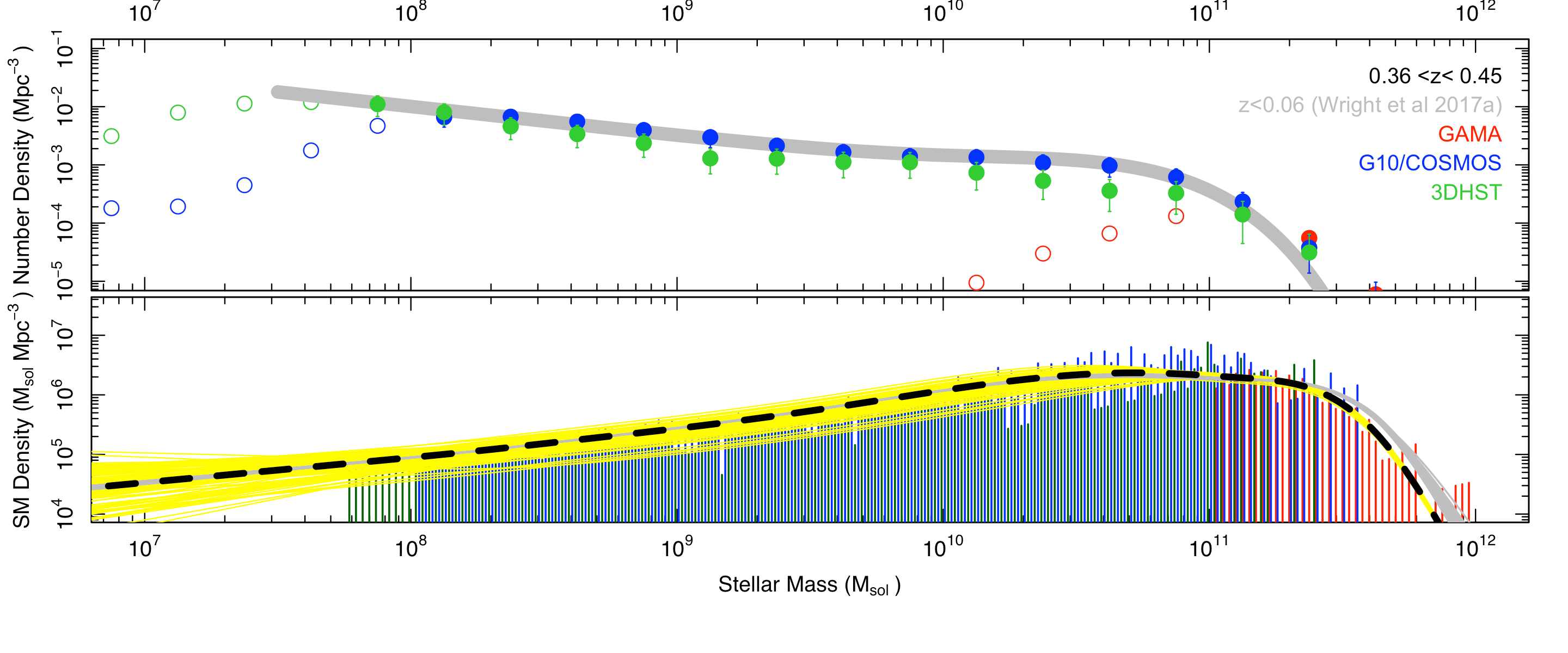
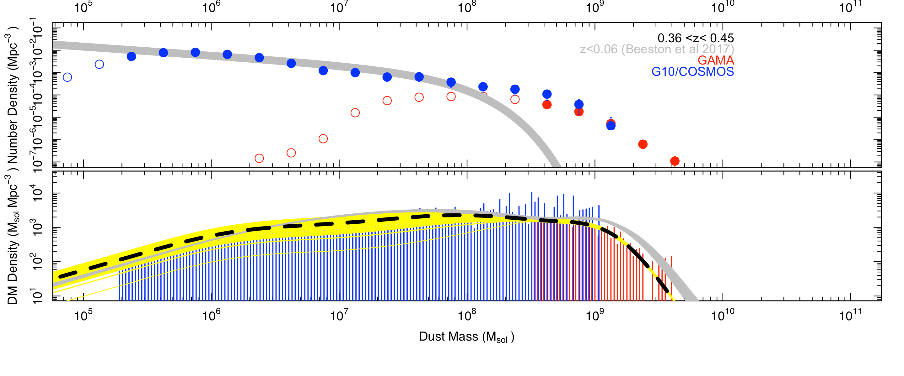
Figure 22: As for Fig. 12 except for the redshift range indicated.

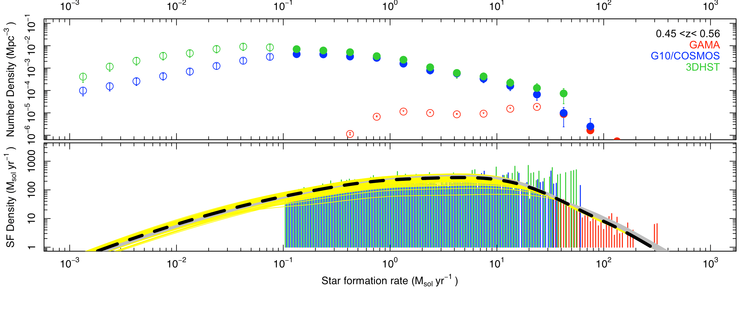
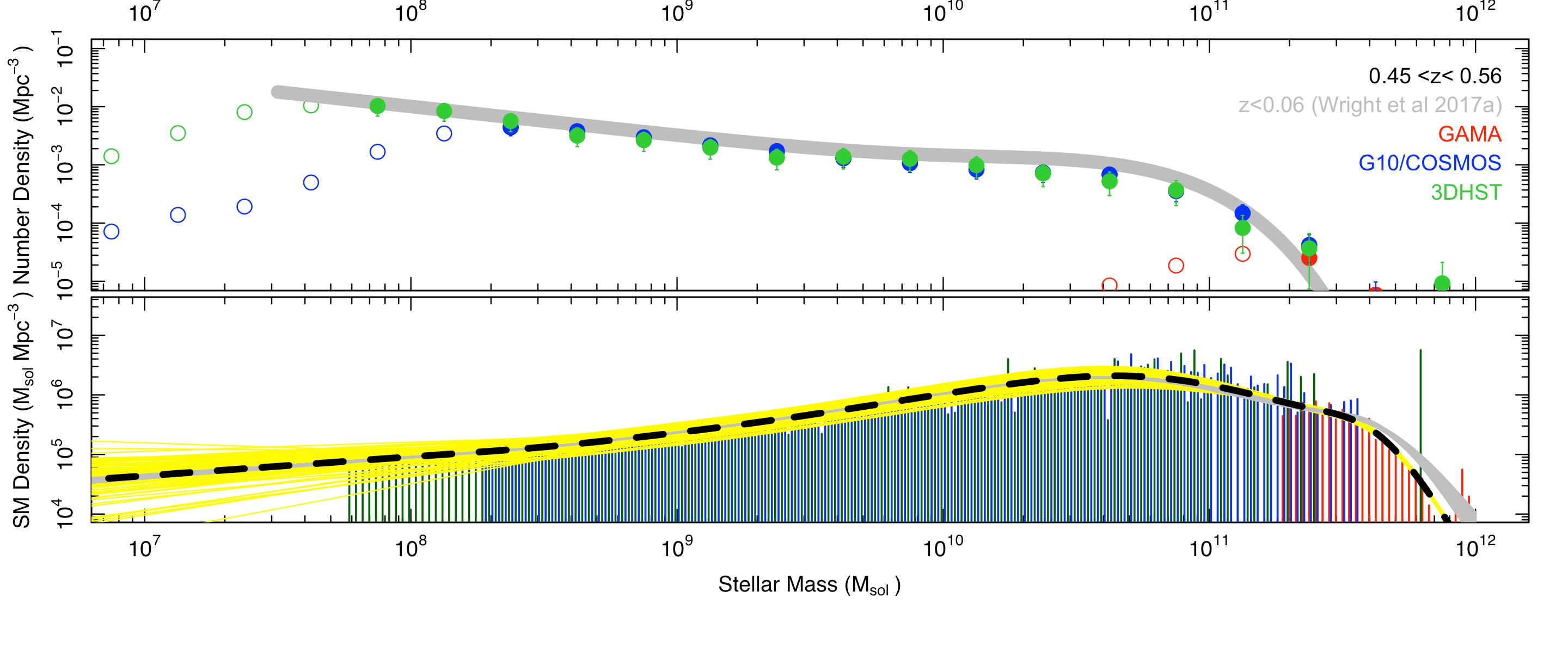
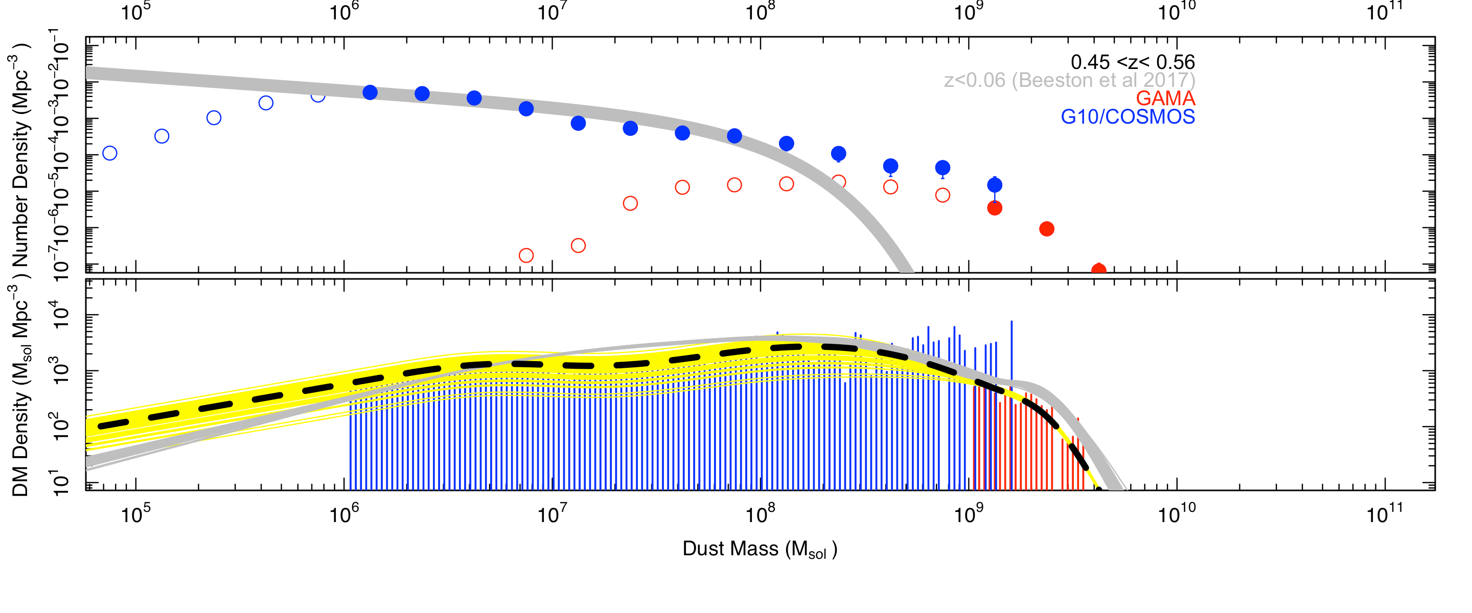
Figure 23: As for Fig. 12 except for the redshift range indicated.

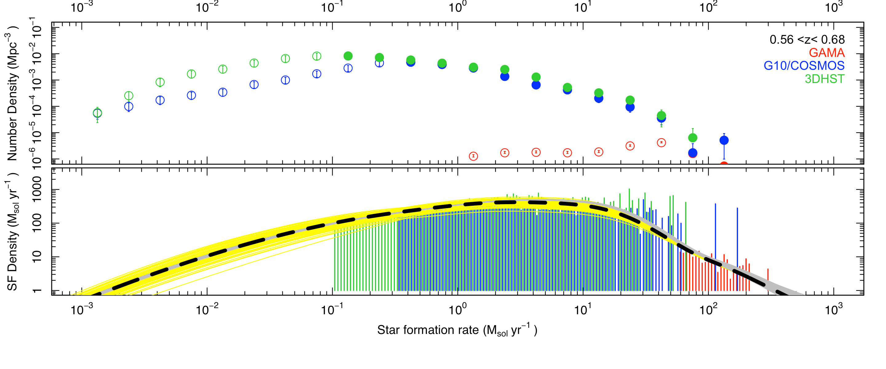
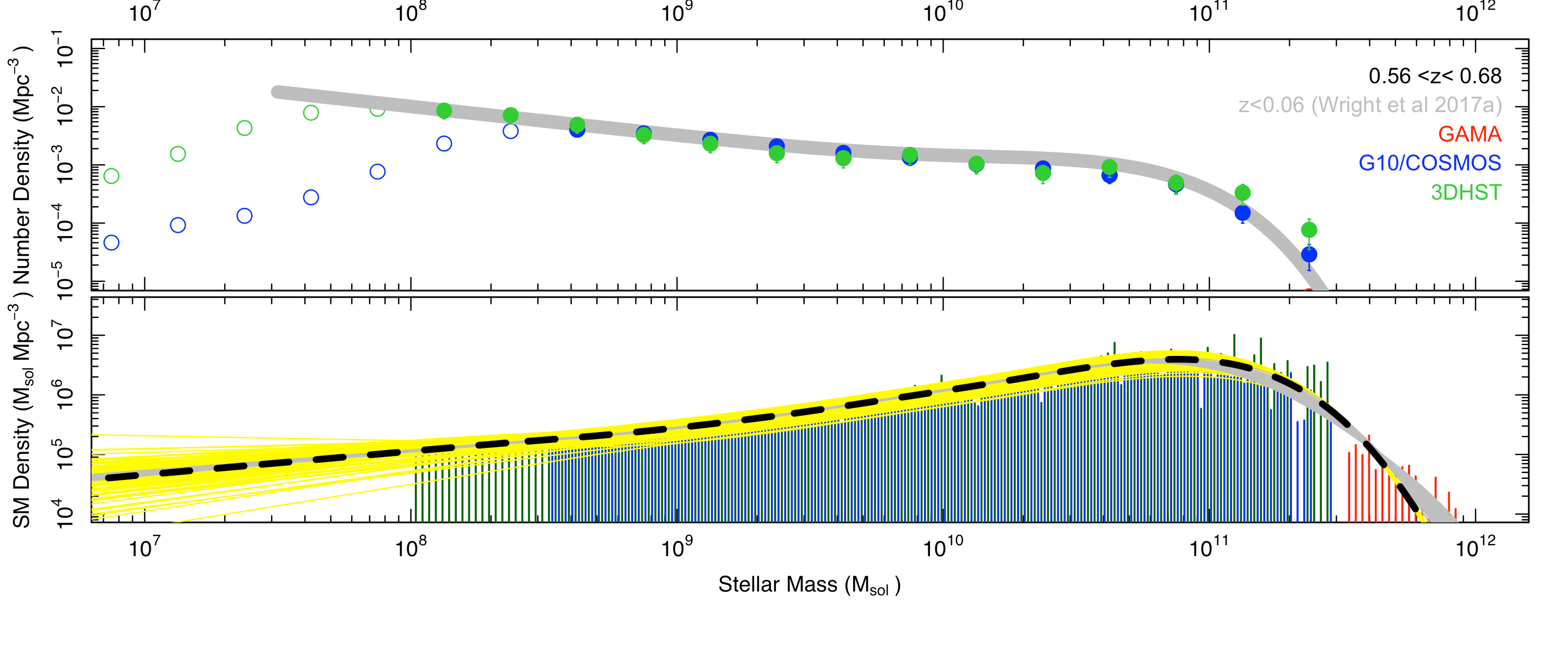
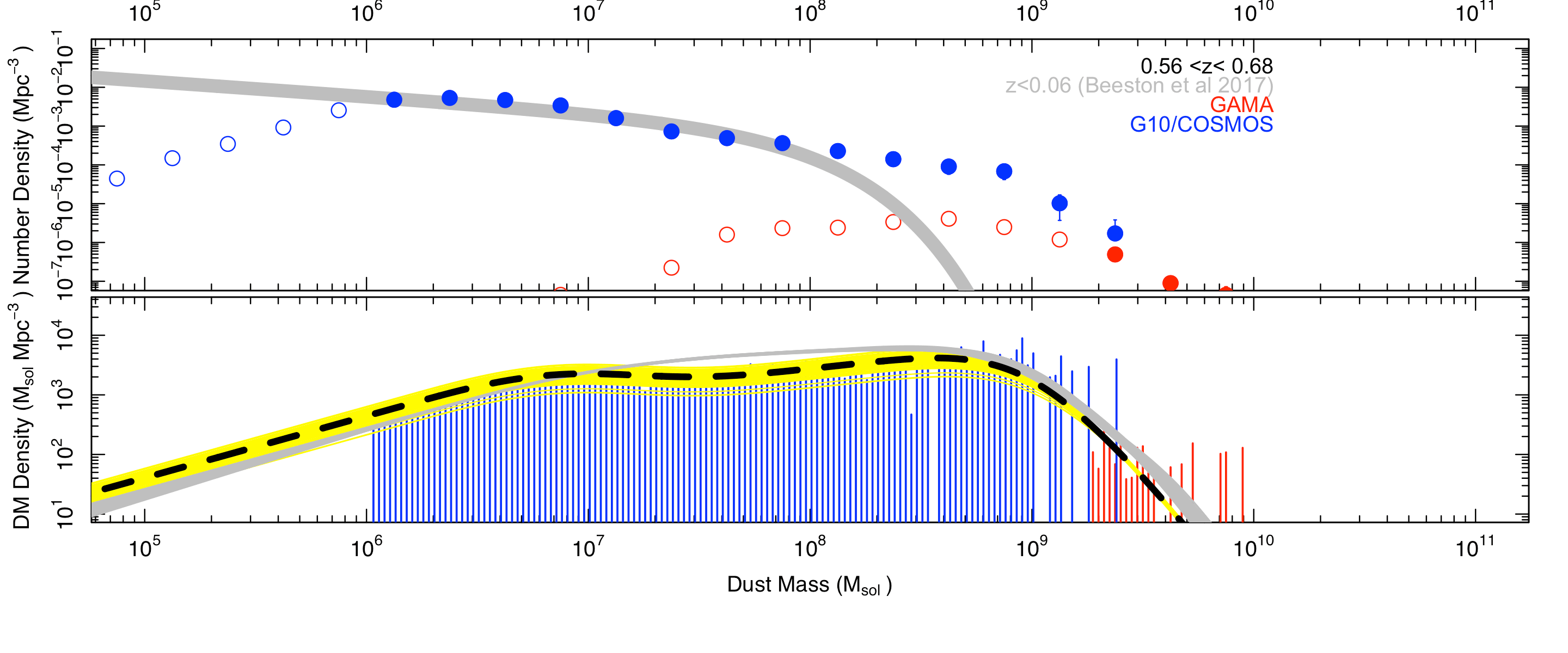
Figure 24: As for Fig. 12 except for the redshift range indicated.

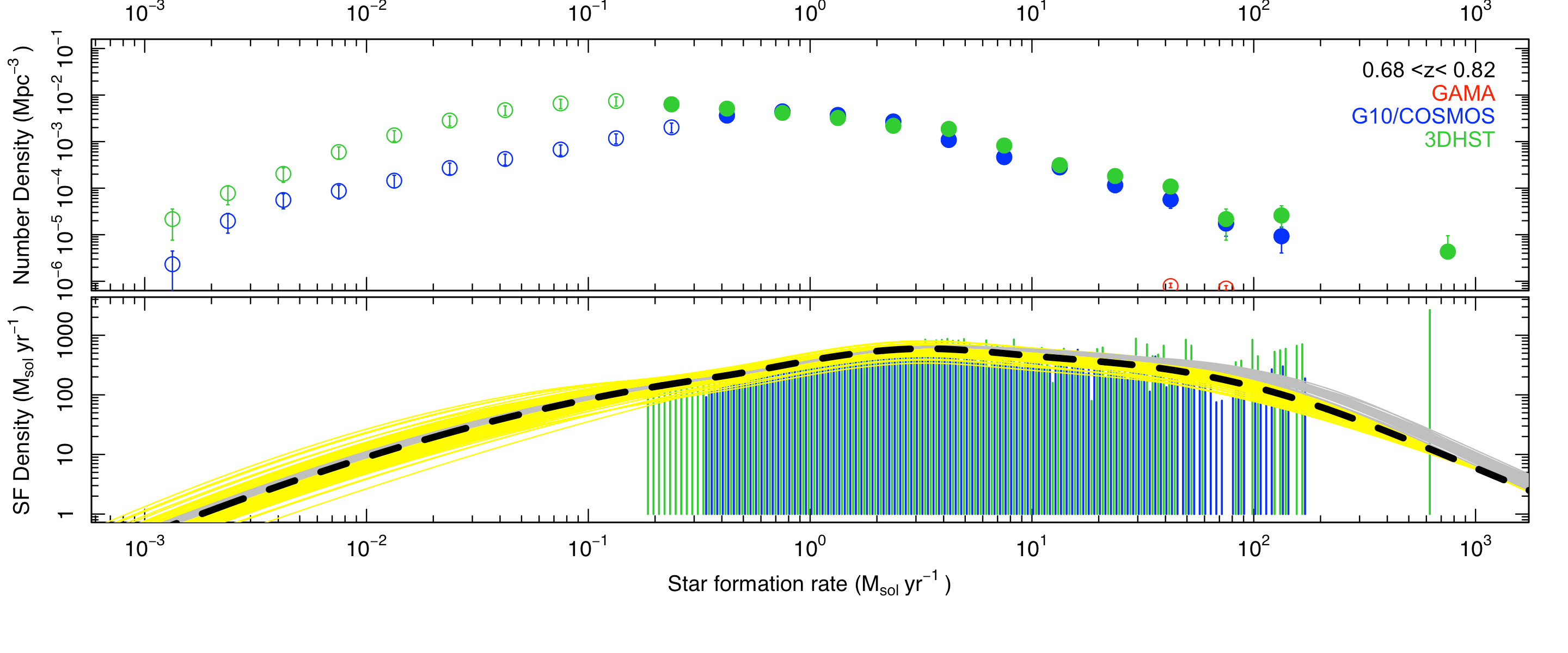
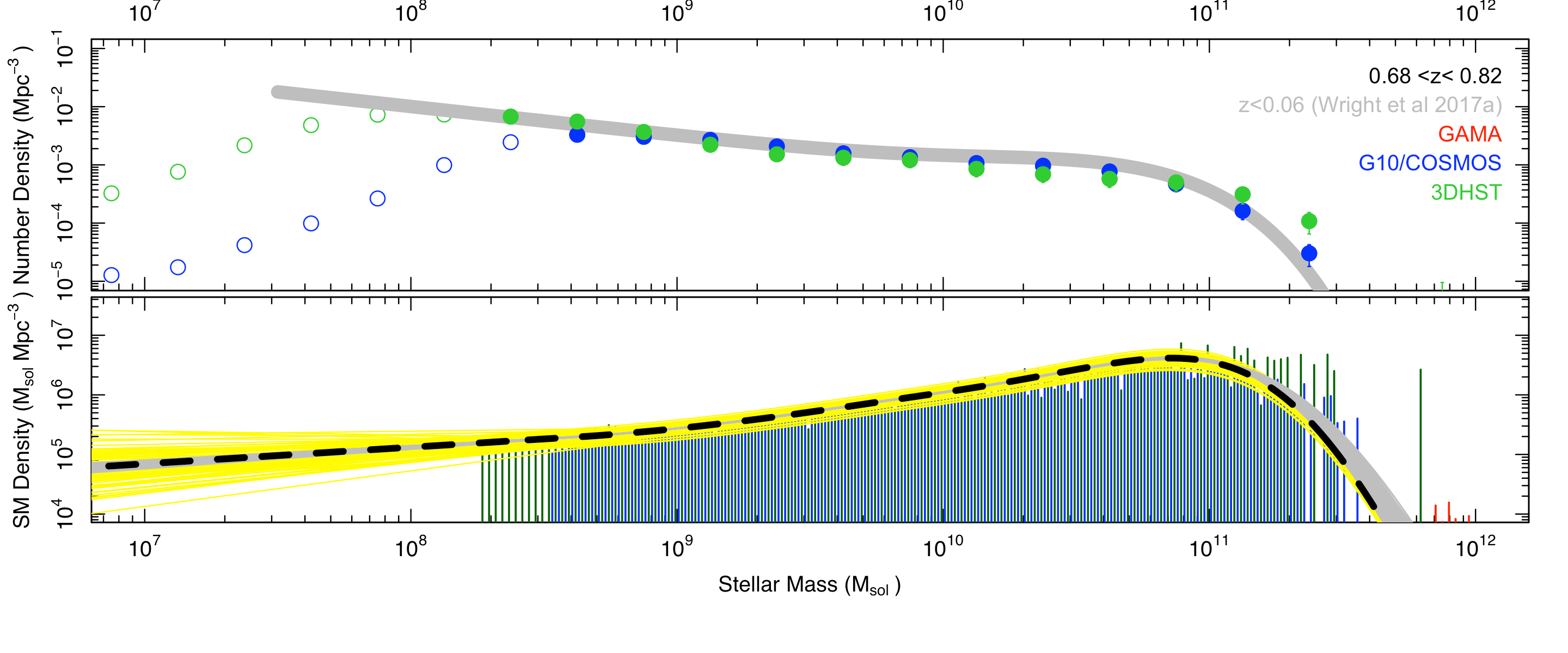
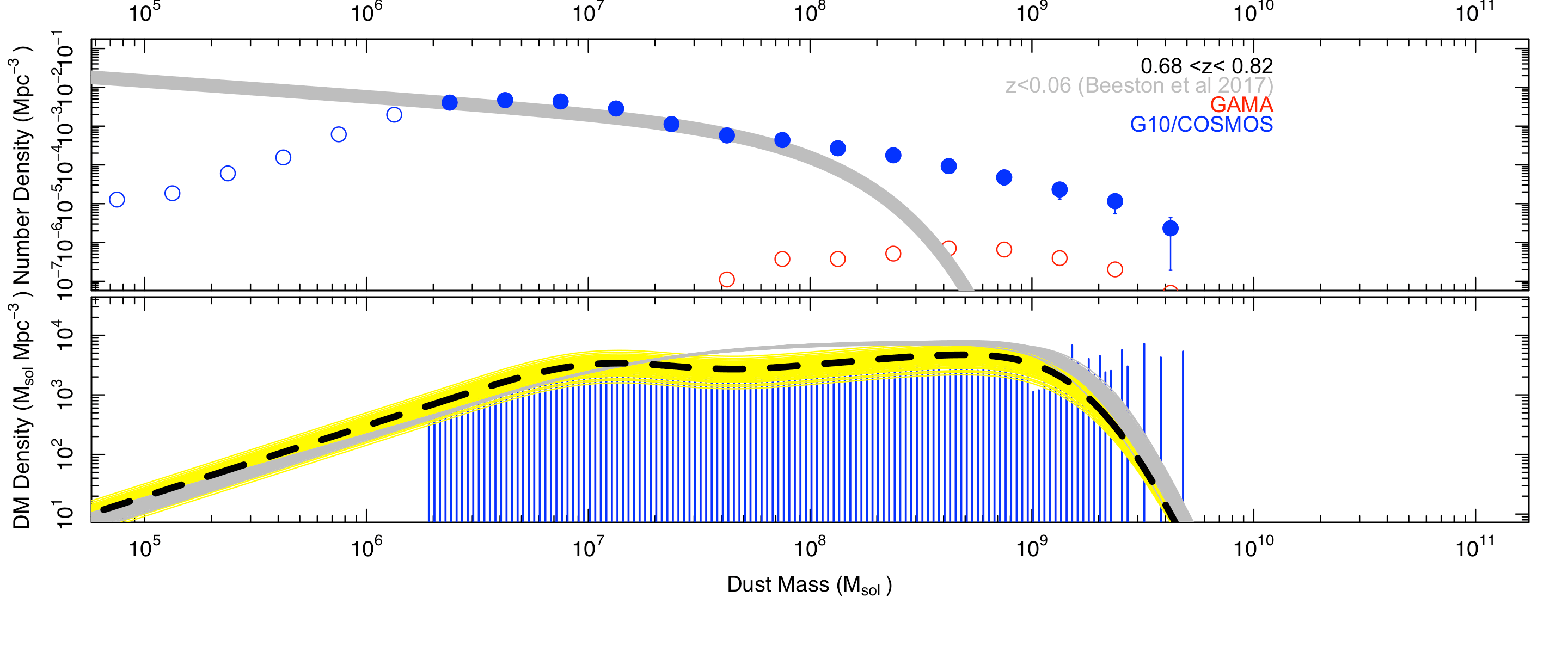
Figure 25: As for Fig. 12 except for the redshift range indicated.

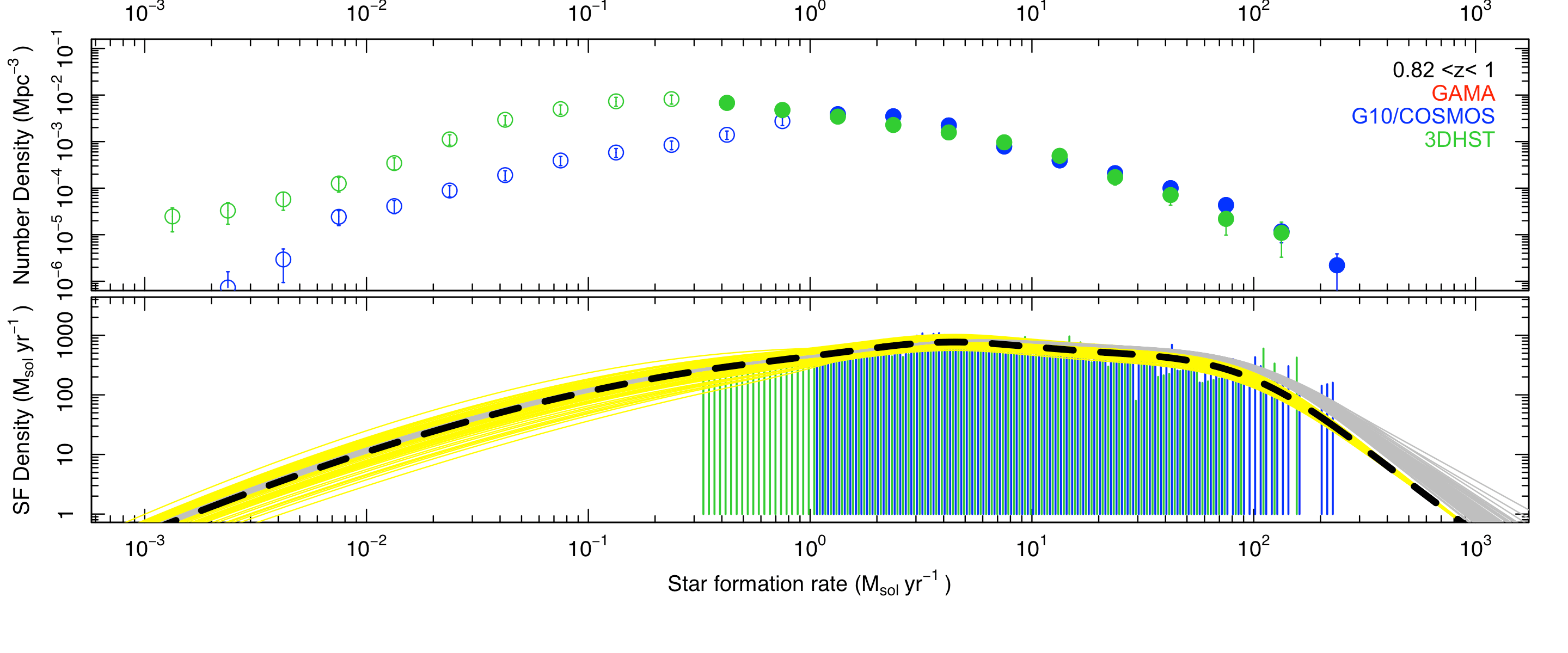
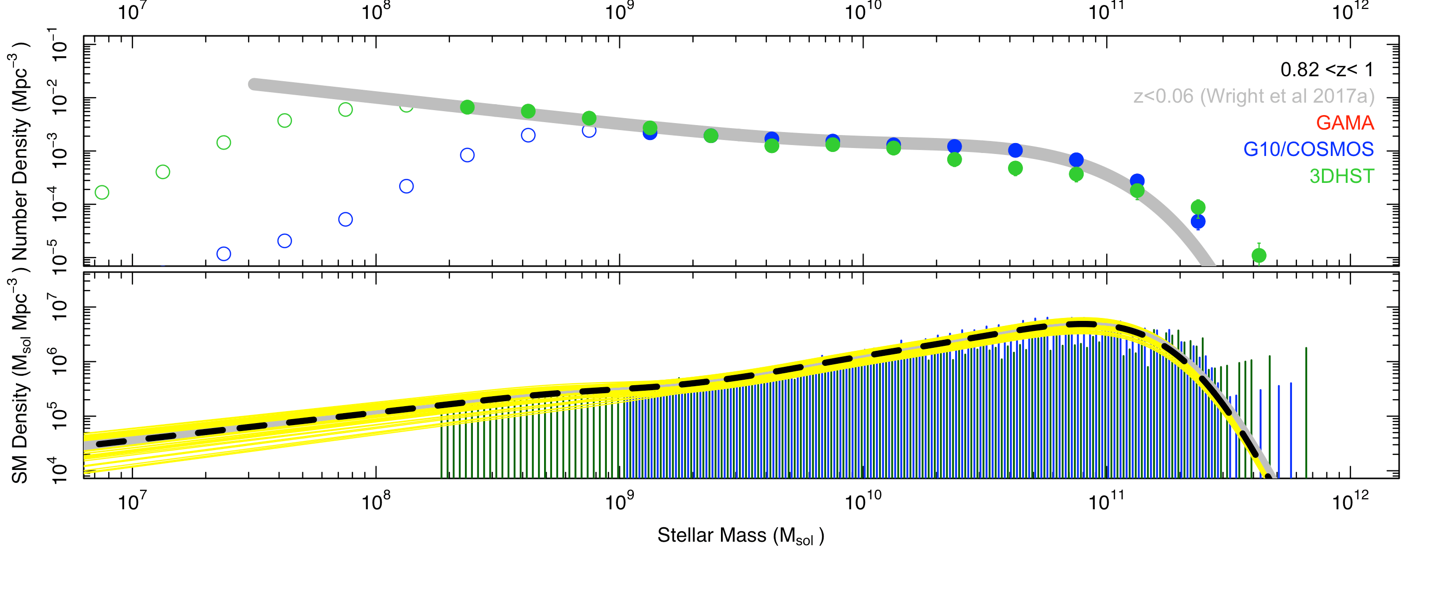
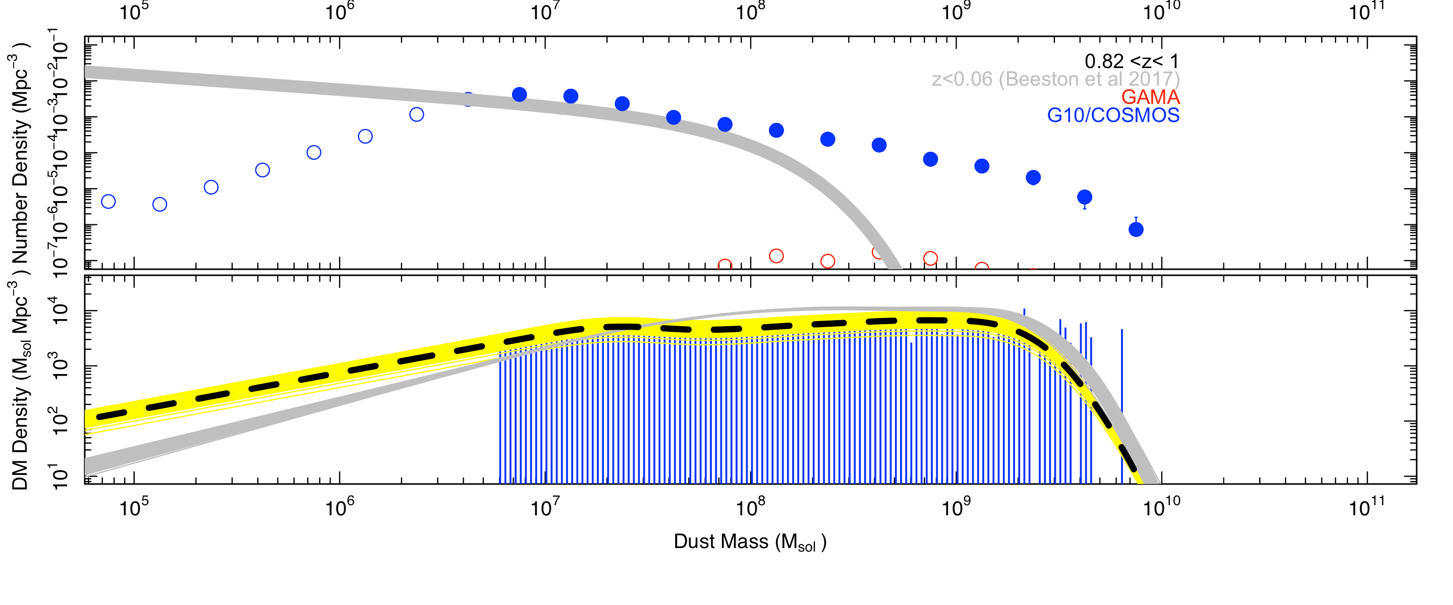
Figure 26: As for Fig. 12 except for the redshift range indicated.

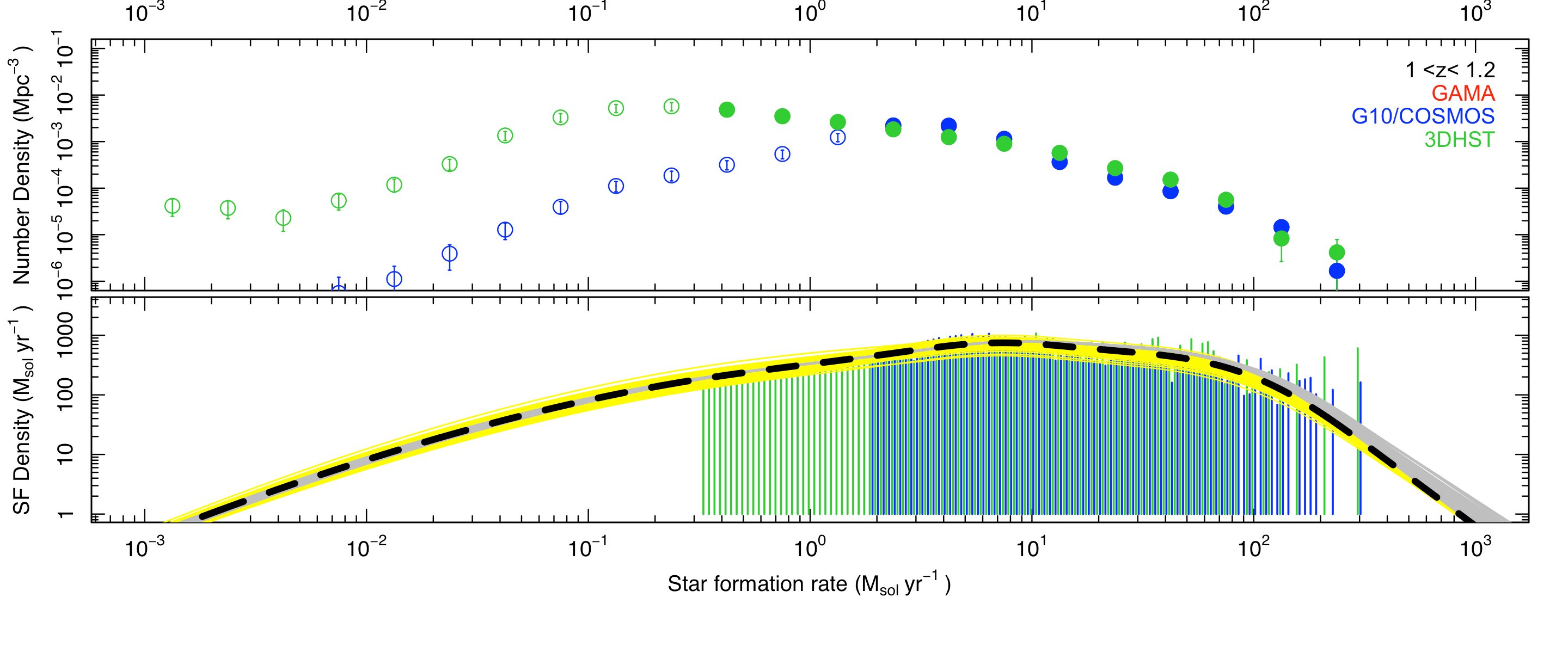
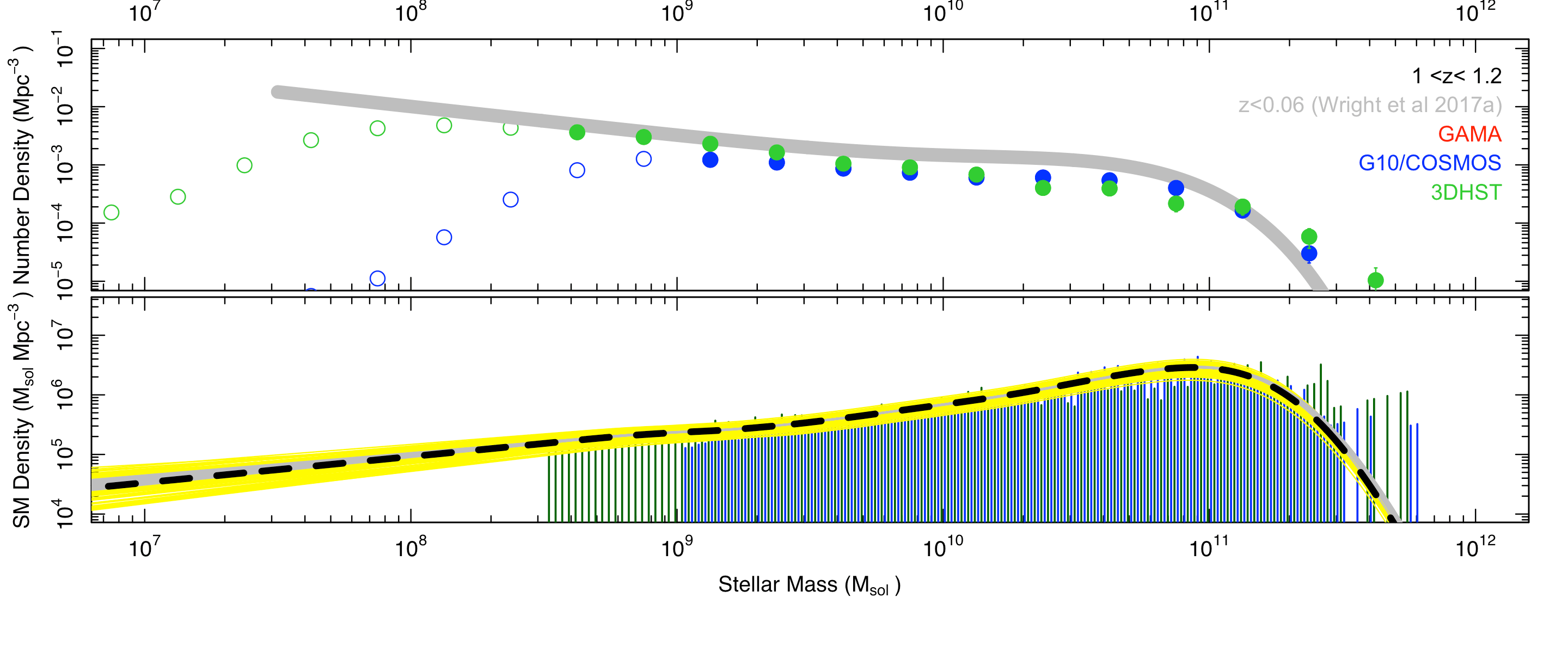
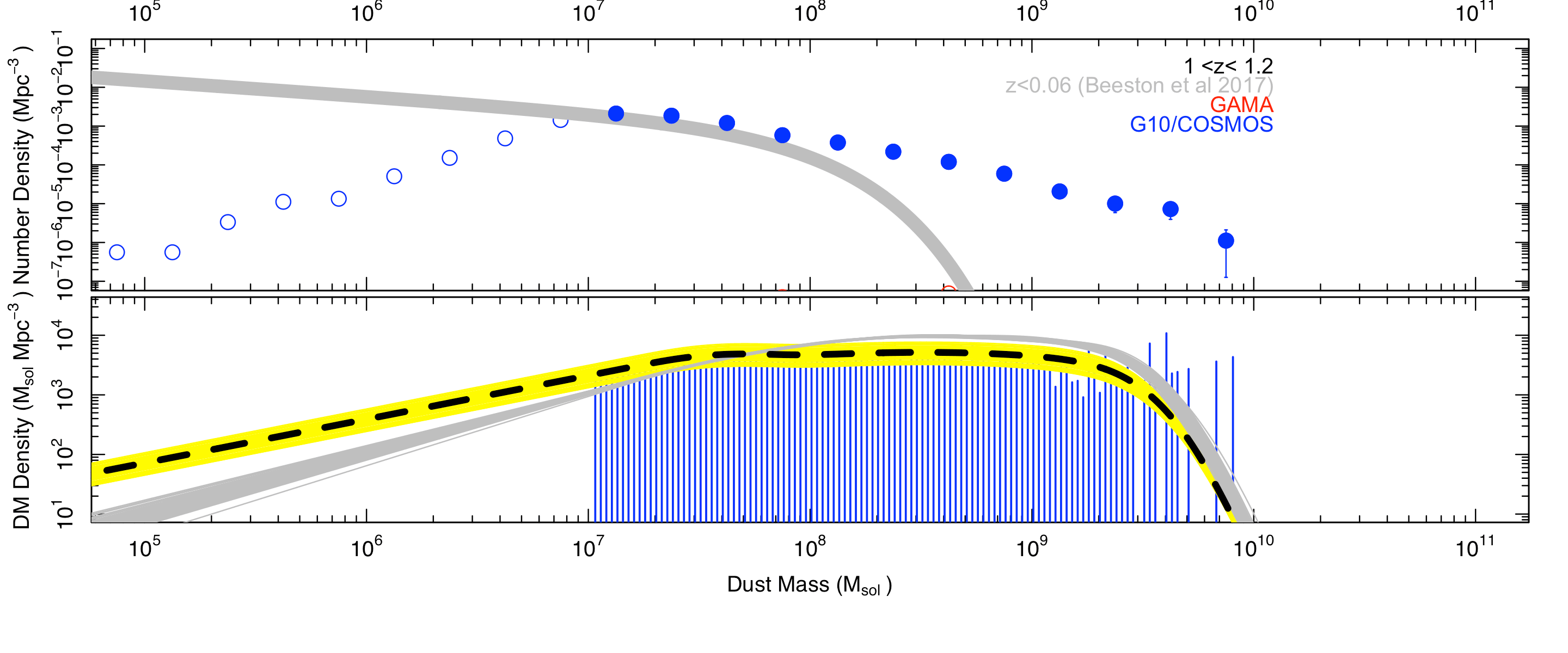
Figure 27: As for Fig. 12 except for the redshift range indicated.

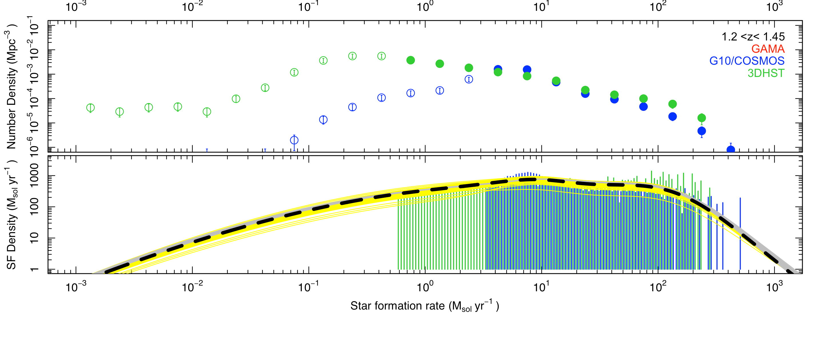
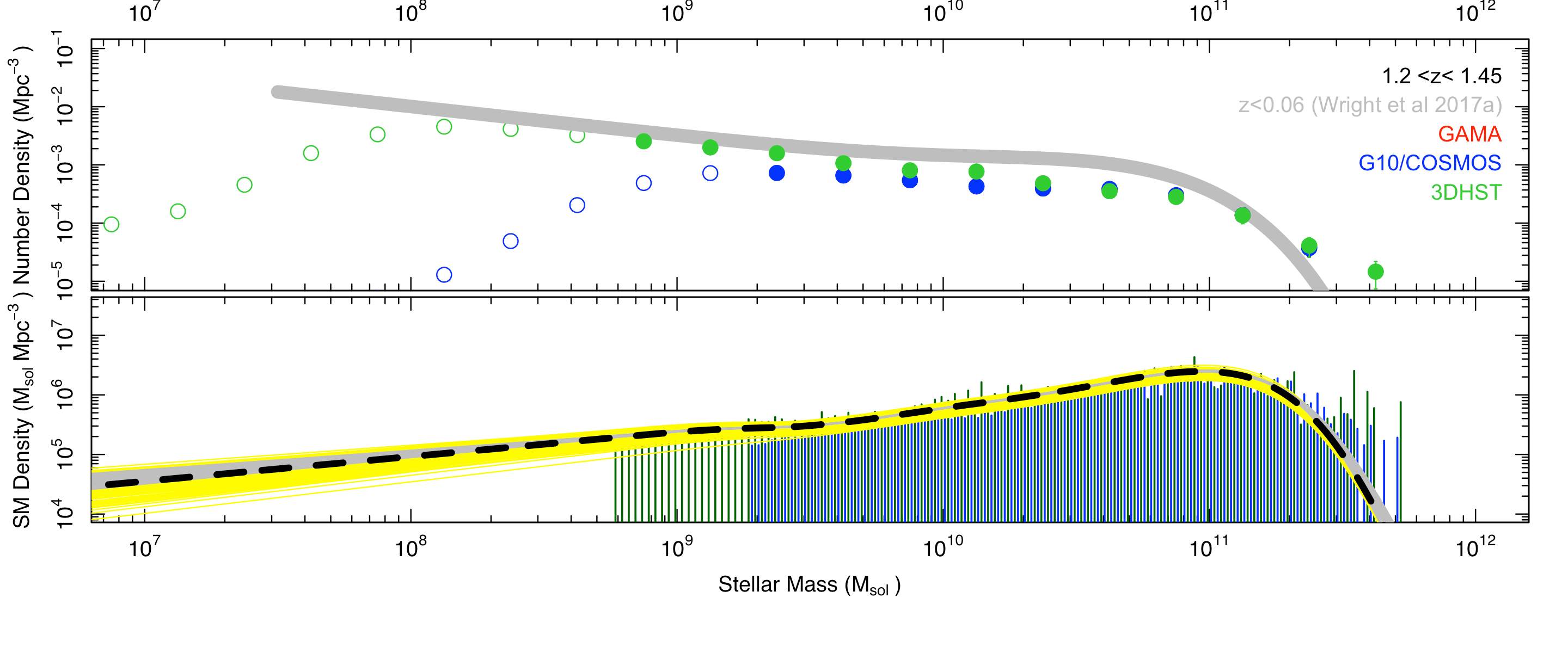
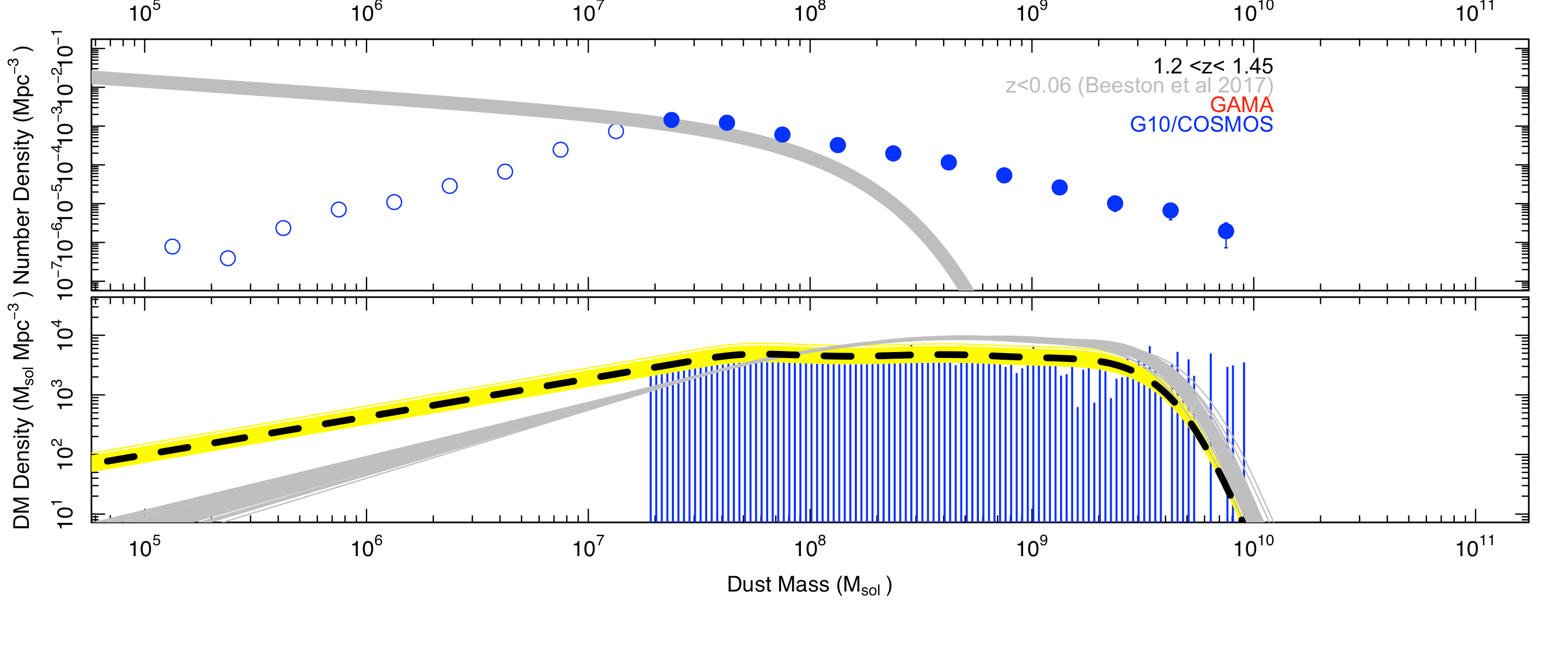
Figure 28: As for Fig. 12 except for the redshift range indicated.

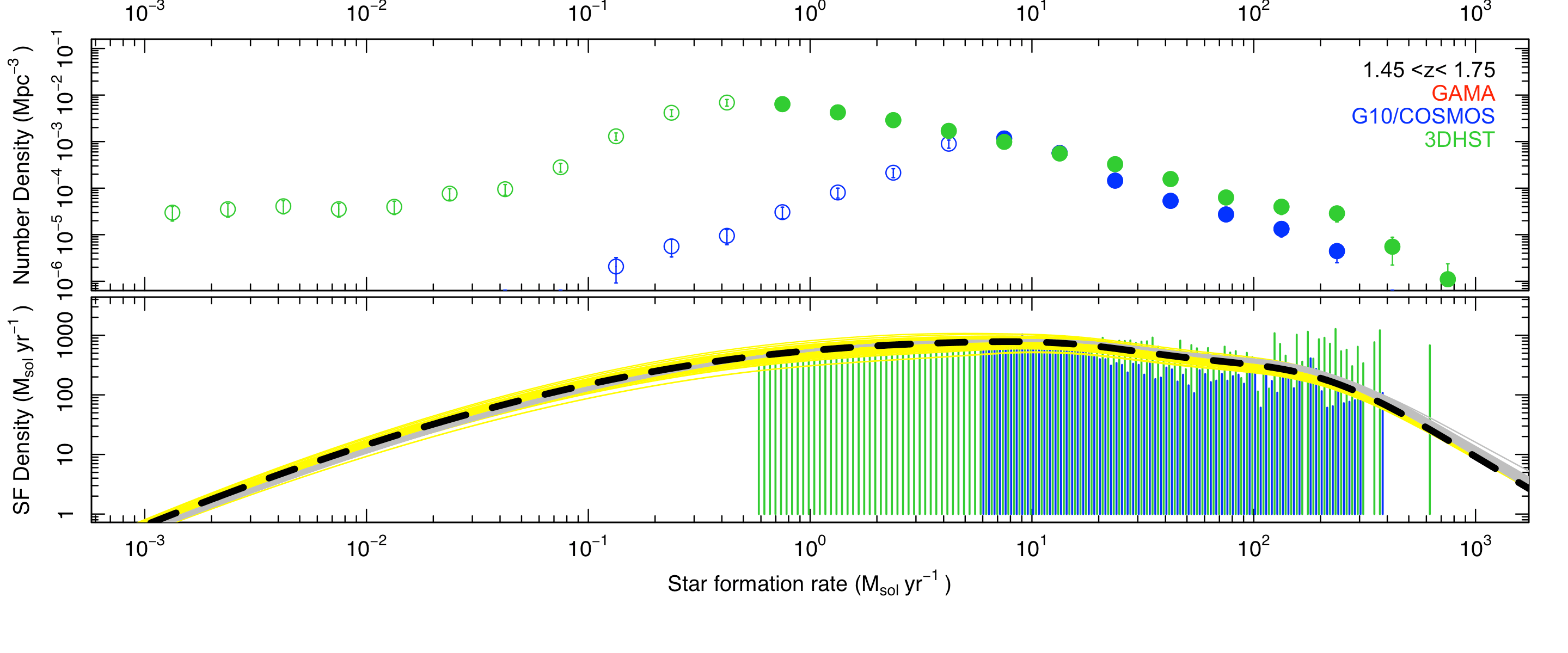
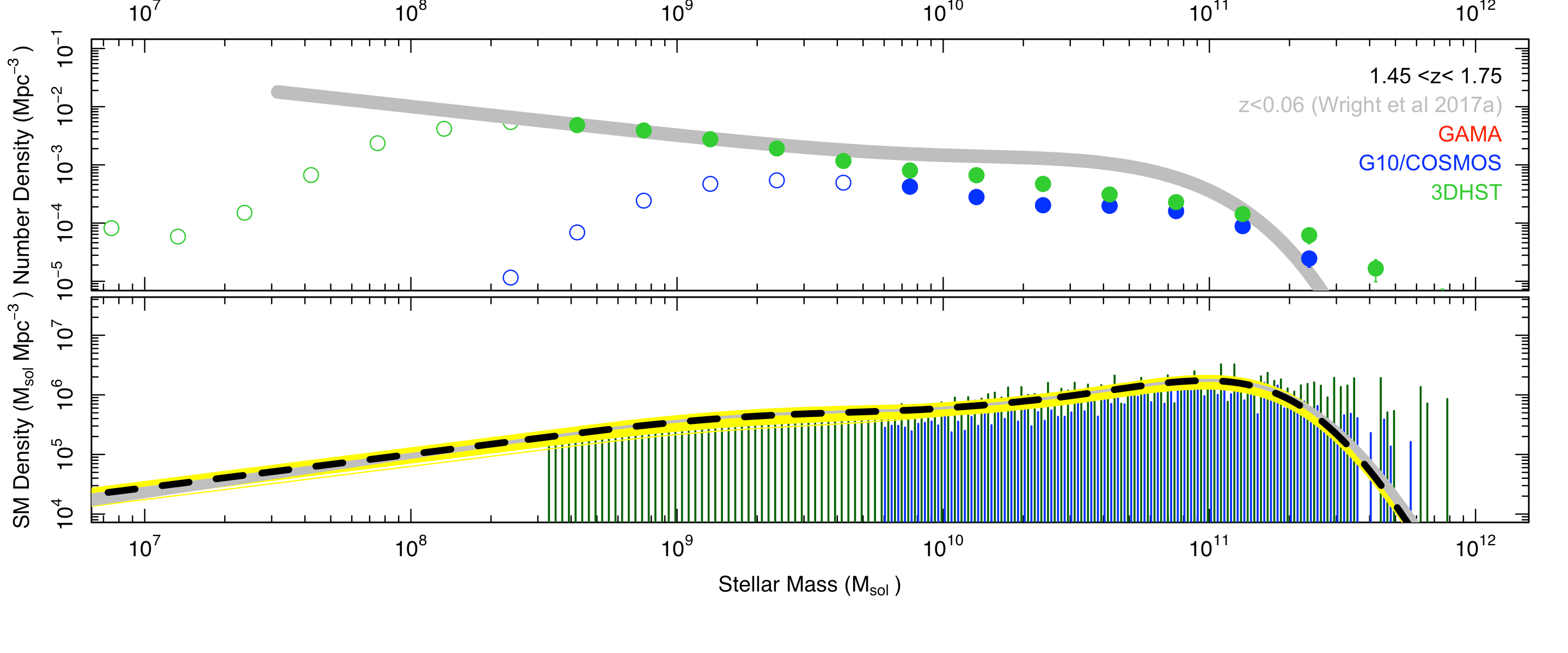
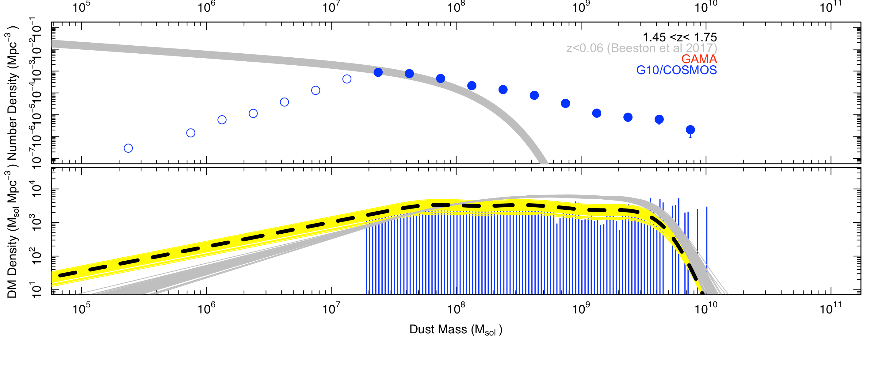
Figure 29: As for Fig. 12 except for the redshift range indicated.

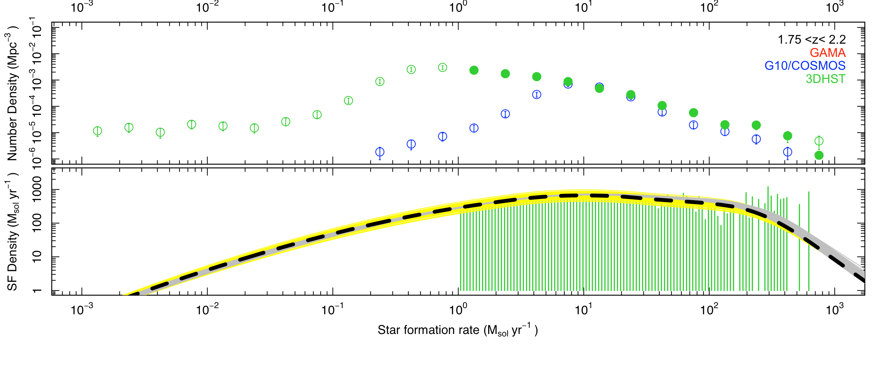
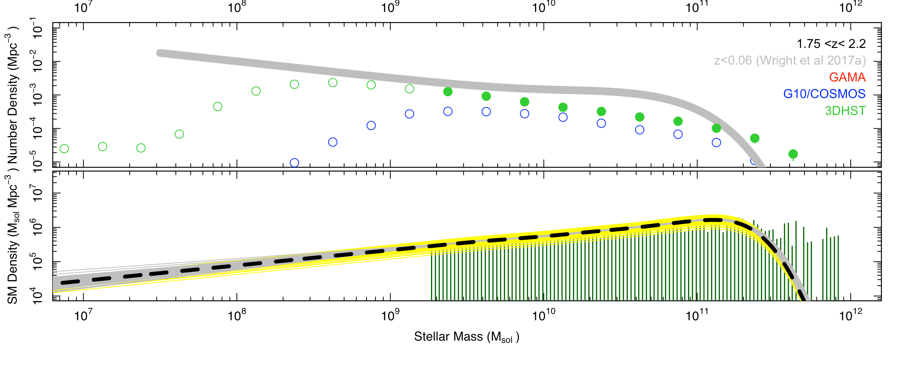
Figure 30: As for Fig. 12 except for the redshift range indicated.

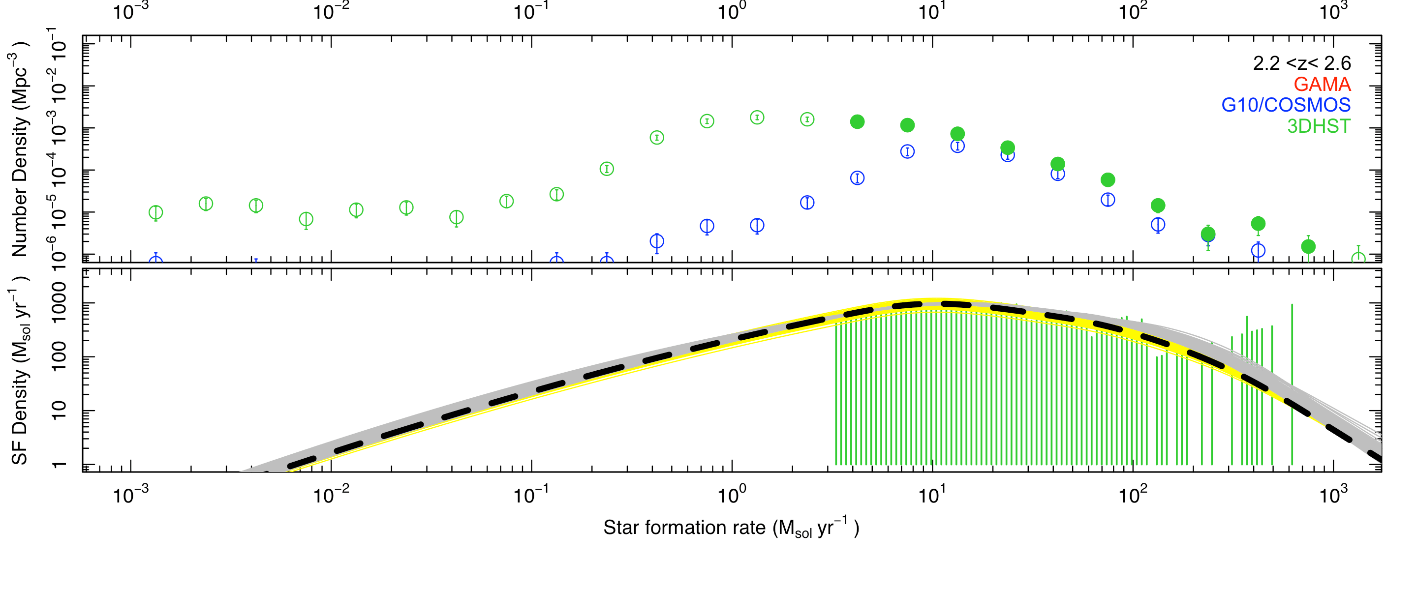
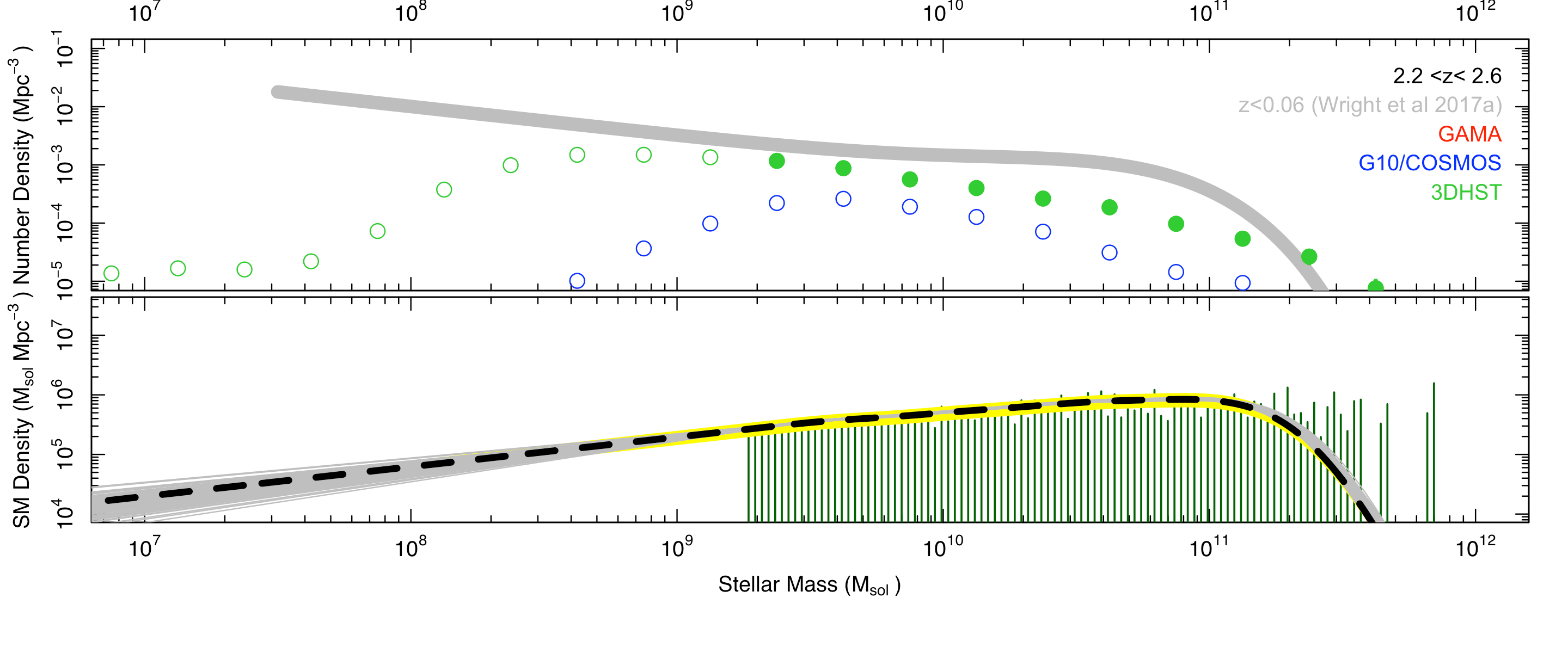
Figure 31: As for Fig. 12 except for the redshift range indicated.

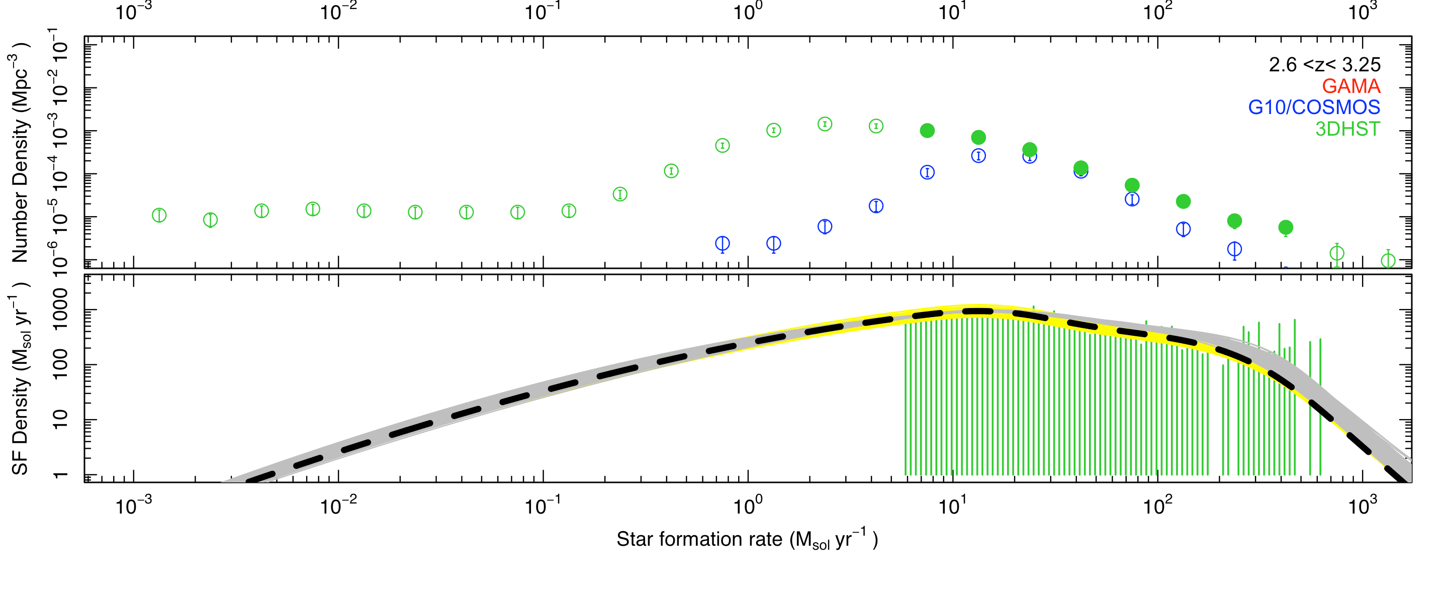
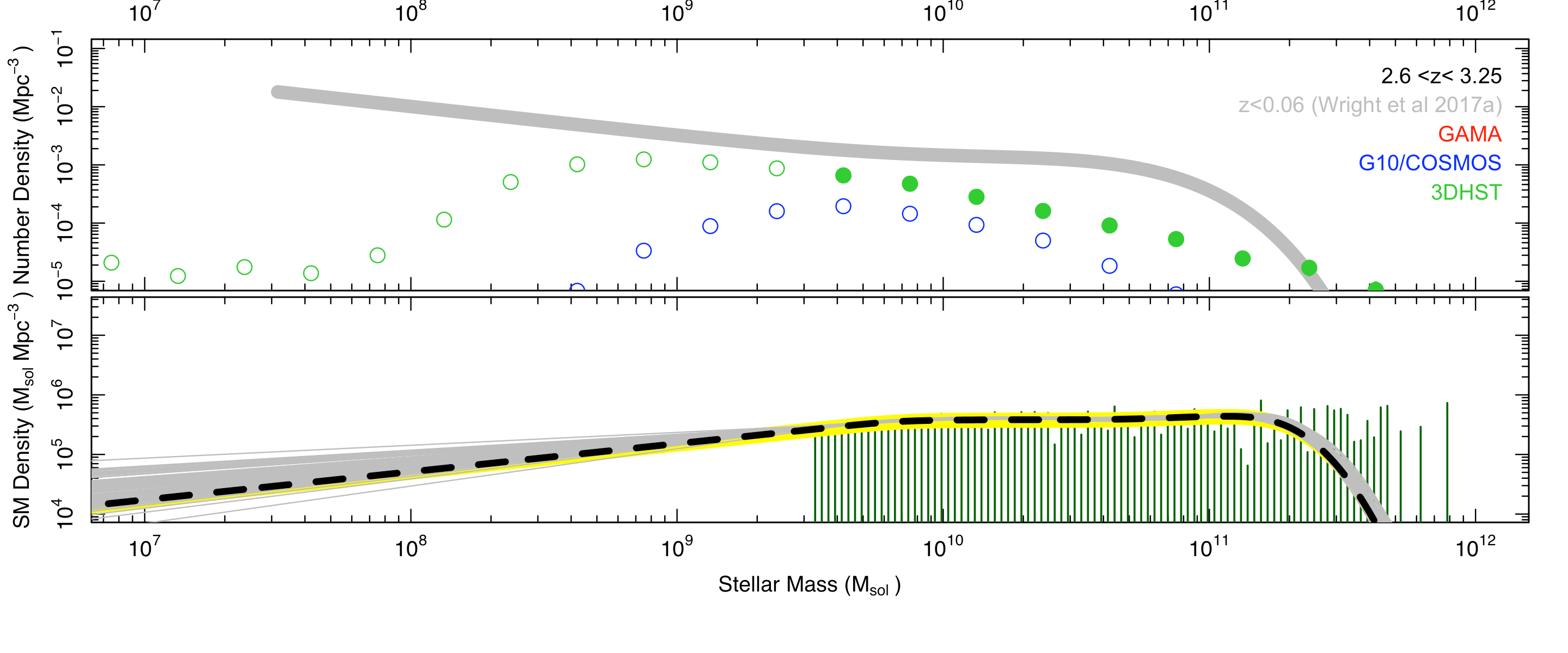
Figure 32: As for Fig. 12 except for the redshift range indicated.

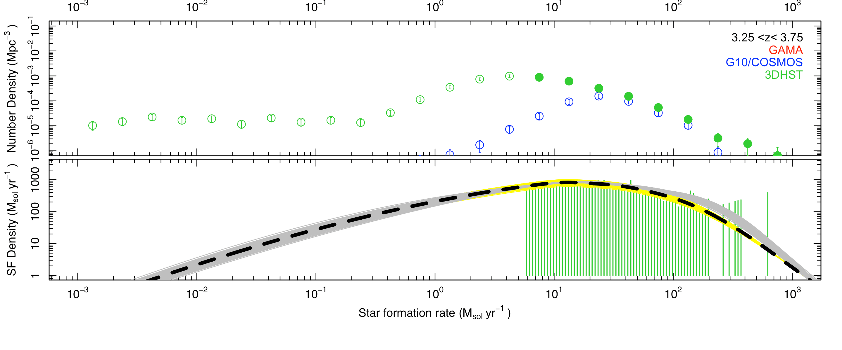
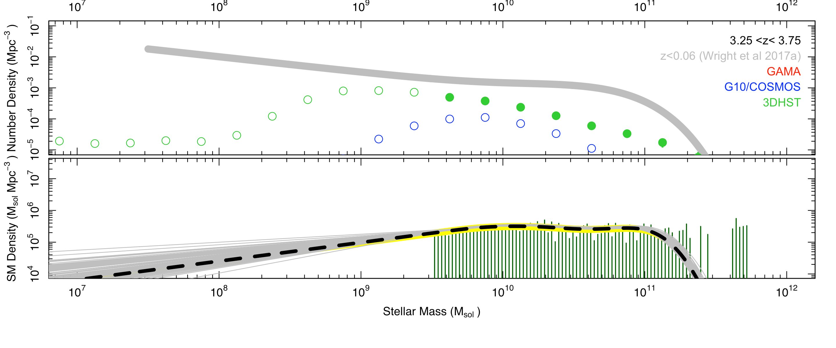
Figure 33: As for Fig. 12 except for the redshift range indicated.

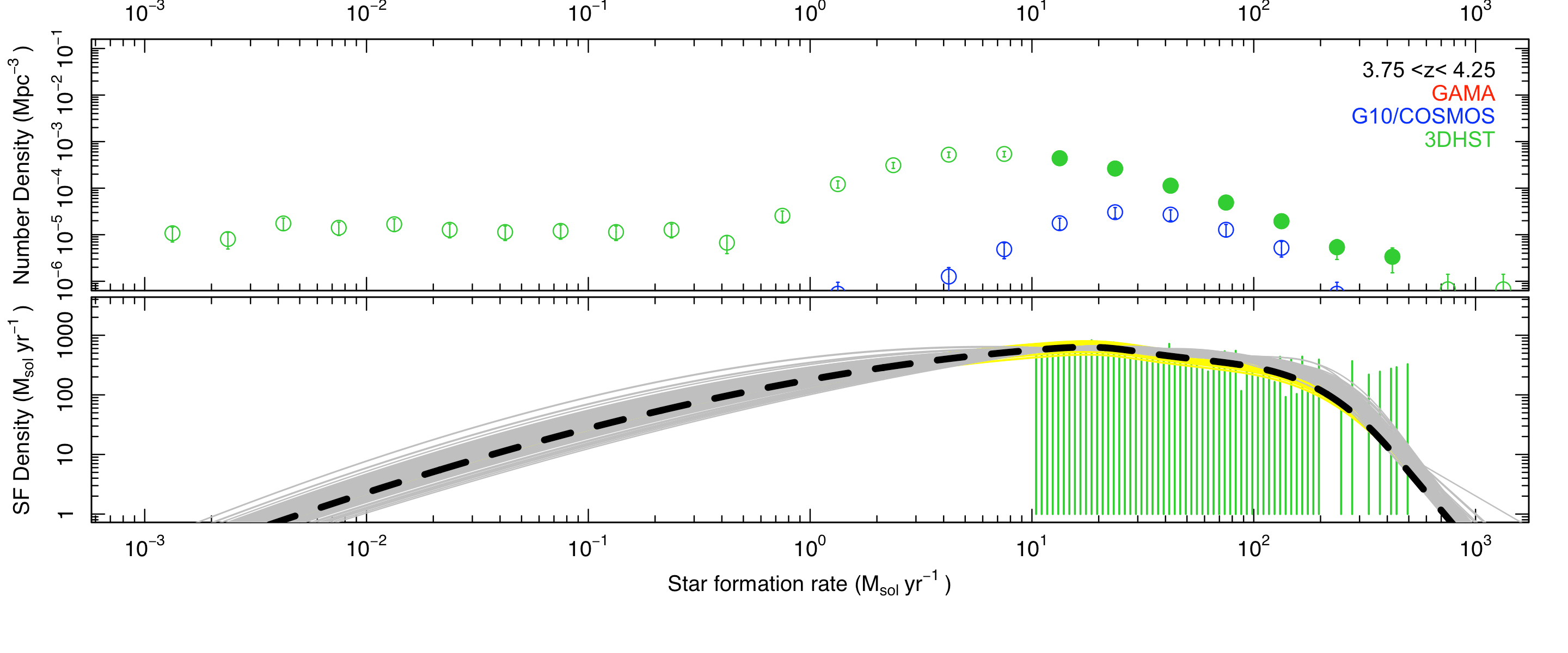
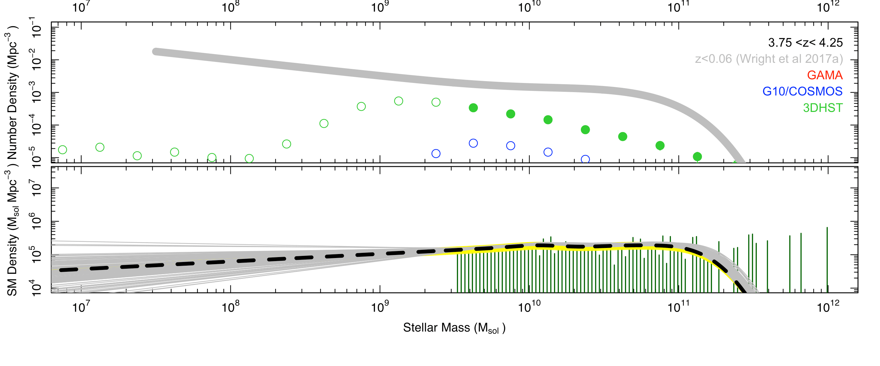
Figure 34: As for Fig. 12 except for the redshift range indicated.

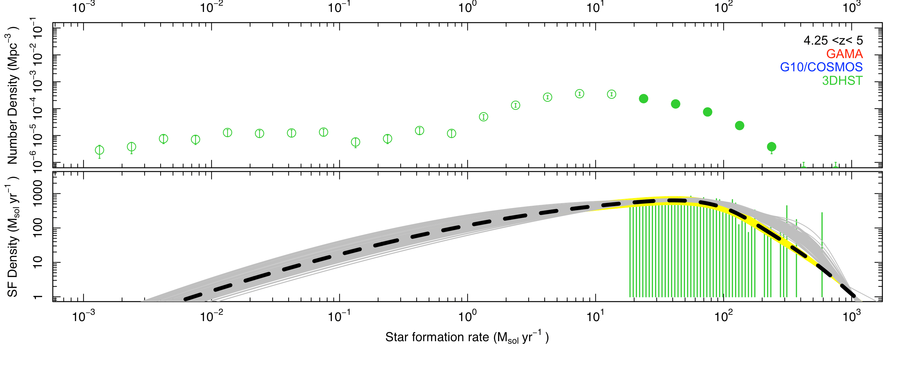
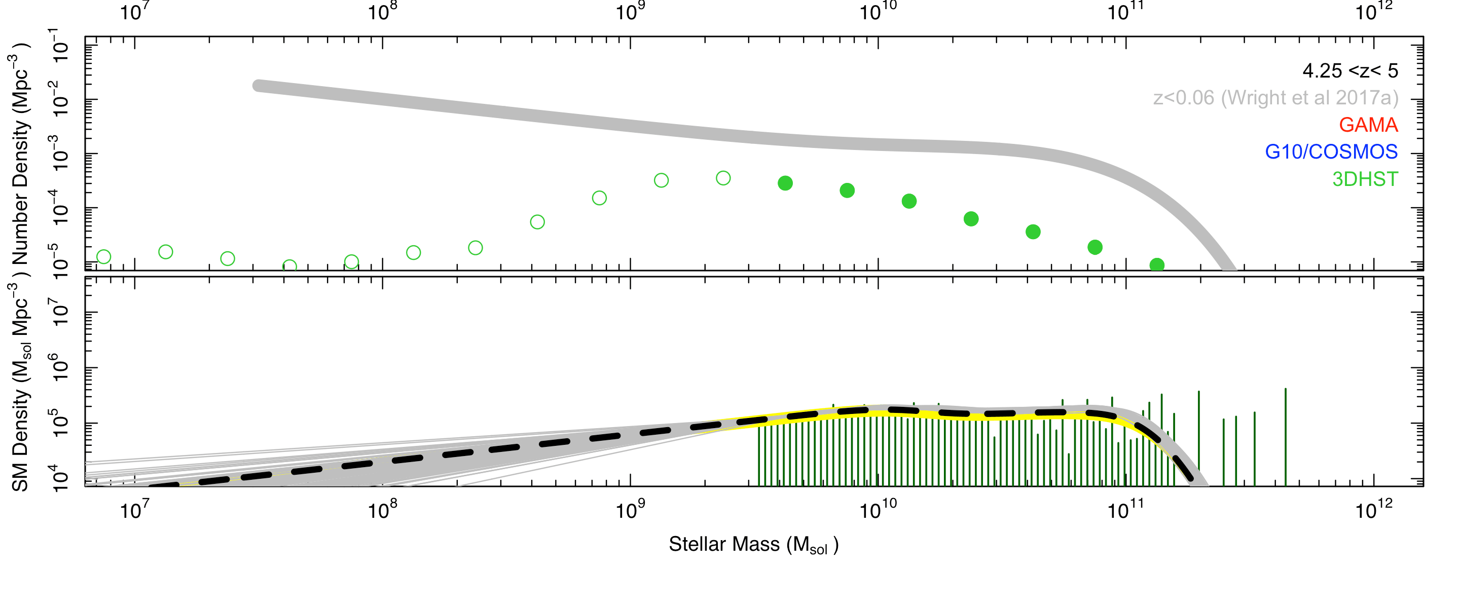
Figure 35: As for Fig. 12 except for the redshift range indicated.

Appendix C CSFH, SMD and DMD versus redshift

For those who prefer to view their data in the highly biased linear redshift plane we include Fig. 36 which replicates the data shown on Fig. 13 but not with a linear redshift axis, which some folk might find useful.

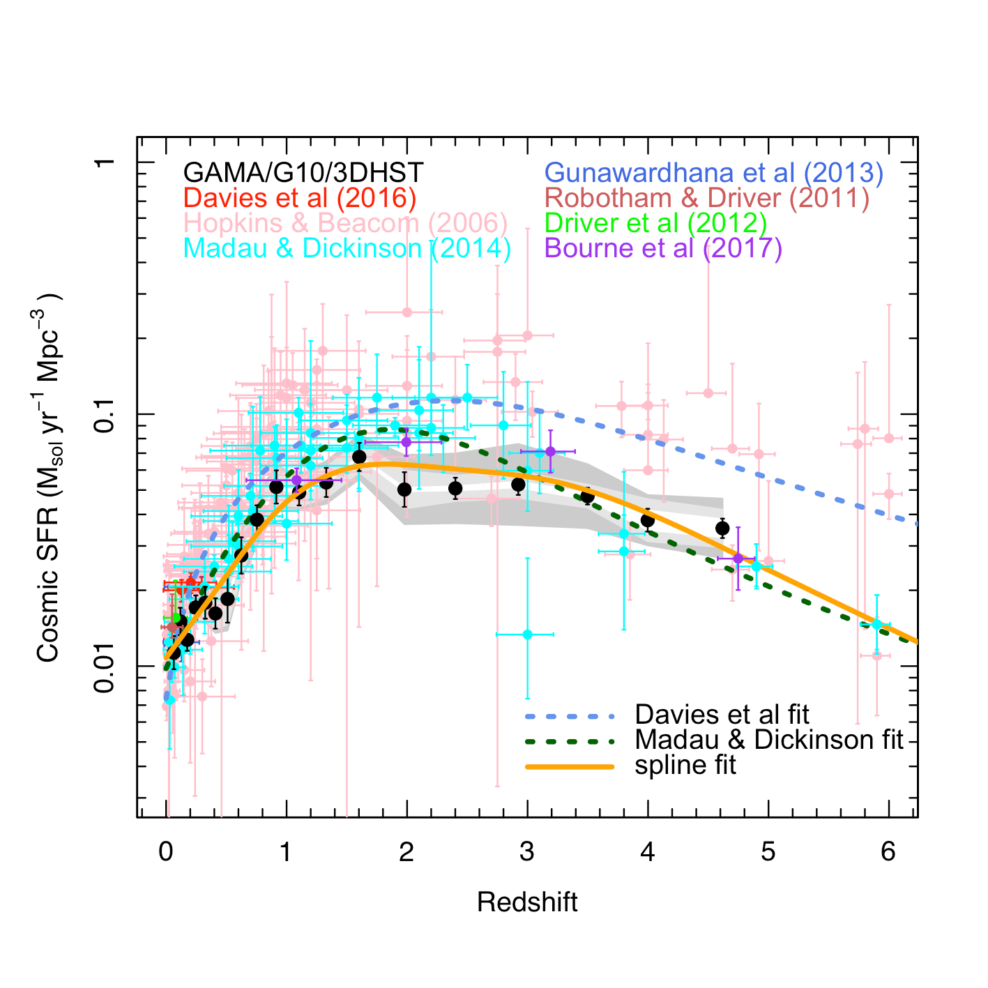
Figure 36: An identical copy to Fig. 13 except with a linear redshift axis for those who prefer to view in a high-z weighted manner.