Boundary behavior of solutions to the parabolic $p$-Laplace equation II

Abstract.

This paper is the second installment in a series of papers concerning the boundary behavior of solutions to the $p$-parabolic equations. In this paper we are interested in the short time behavior of the solutions, which is in contrast with much of the literature, where all results require a waiting time. We prove a dichotomy about the decay-rate of non-negative solutions vanishing on the lateral boundary in a cylindrical $C^{1,1}$ domain. Furthermore we connect this dichotomy to the support of the boundary type Riesz measure related to the $p$-parabolic equation in NTA-domains, which has consequences for the continuation of solutions.

1. Introduction

Recently there has been an upsurge in progress concerning the boundary behavior of solutions to the $p$-parabolic equation [1, 2, 3, 4, 5, 7, 8, 12].

Before our paper [2] the behavior of solutions close to the boundary was largely unknown in excess of regularity estimates, in [2] we proved a Carleson estimate for Lipschitz domains and also pointed out that in the degenerate regime ($p>2$), the failure of forward Harnack chains stems from the possible decay of certain solutions near the boundary, bounded by $d(x,\partial\Omega)^{q}$ for $q\geq\frac{p}{p-2}$. In [2] we also noted that the boundary Harnack inequality cannot be true in the same form as for $p=2$, however in [3] we proved that if the solutions have existed for long enough then the boundary Harnack inequality holds. This was a major breakthrough, but understanding of how badly the boundary Harnack can fail for shorter time-scales was still lacking. The purpose of this paper is to bridge this gap by proving exactly how badly the boundary Harnack inequality fails. We do this by studying the decay-rate of solutions that vanish on the boundary and discover a certain decay-rate phenomenon, a dichotomy, that only occurs in the degenerate regime. To describe this phenomenon we first state our equation

$$u_{t}-\Delta_{p}u=u_{t}-\nabla\cdot(|Du|^{p-2}Du)=0,\quad p>2,$$ (1.1)

we call 1.1 the degenerate $p$-parabolic equation. The phenomenon consists of two related observations, first of all is the existence of solutions with different decay rates close to the boundary, let us illustrate with an example. Let $T\in{\mathbb{R}}$, then in ${\mathbb{R}}_{+}^{n}\times(-\infty,T)$ consider

$$u_{1}(x,t) =C(p)(T-t)^{-\frac{1}{p-2}}x_{n}^{\frac{p}{p-2}}.$$ (1.2)

Another solution which we simply obtain is $u_{2}=x_{n}$, the point is that $u_{1}$ and $u_{2}$ behave very differently at the boundary and shows, for instance, that a short time boundary Harnack inequality cannot hold. That is the ratio

$$\frac{u_{2}}{u_{1}}\qquad\text{is not bounded from above and below.}$$

Another observation concerning the solution in 1.2 is that the solution is exactly so small that one cannot build Harnack chains up to the boundary, as noted in [2]. In fact for the $p$-parabolic equation, the waiting time for $u_{1}$ dictated by the Harnack inequality at a point $(x_{0},t_{0})$ is

$$C(T-t_{0})x_{0}^{-p}r^{p}.$$

This implies that if we wish to apply the Harnack inequality with a radius comparable to the distance to the boundary then the waiting time will be of the same order of magnitude as the distance from $t_{0}$ to $T$ (the end of existence), in essence this implies that a Harnack chain cannot be performed.

The other aspect is that solutions retain some of the behavior of the initial data in the sense described by the following example from [2]. That is, consider the following supersolution to 1.1

$$u(x,t)=C(p)(T-t)^{-\frac{1}{p-2}}\exp(-\frac{1}{x}),\qquad x\in(0,1/4).$$

It is now clear that if our domain is $E_{T}=(0,1)\times(0,T]$ then the Cauchy-Dirichlet problem in $E_{T}$ has a short time behavior that is heavily dictated by the decay of the initial data, in contrast to the linear case, where no matter what positive data we have we will always have that $\partial_{x}u(0,t)>0$ for all $t\in(0,T)$. We explore this “memory effect” further in Section 6.

Our prime motivating idea is that the existence of a forward Harnack chain should imply that the equation behaves like a non-degenerate equation, in the sense that there would be no memory effect and there can only exist one behavior at the boundary, i.e. solutions vanish like the distance function. We can state this simply as, there should be no solution that vanishes slower than $u_{1}$ in 1.2 and at the same time, faster than $u_{2}=x_{n}$. To state this precisely we need to introduce some concepts, we start with the definition of a degenerate boundary point

Definition 1.1.

Let $\Omega\subset{\mathbb{R}}^{n}$ be a domain and let $u$ be a solution to 1.1 in $\Omega_{T}=\Omega\times(0,T)$. We call $w\in\partial\Omega$ a degenerate point at $t_{0}\in(0,T)$ with respect to $u$ if

$$\mathcal{N}^{+}\left[\frac{u(x,t_{0})}{|x-w|^{\frac{p}{p-2}}}\right](w)<\infty,$$

where

$$\mathcal{N}^{+}[f](w) =\limsup_{x\in\Gamma(w),x\to w}f(x)$$

$$\Gamma_{\alpha}(w) =\left\{x\in\Omega:\alpha|x-w|<d(x,\partial\Omega)\right\}$$

for some $\alpha\in(0,1)$.

Remark 1.2.

The value of $\alpha>0$ in the above definition does not enter into any of the estimates and is irrelevant as long as $\Gamma(w)$ satisfies

$$\Gamma(w)\cap B_{r}(w)\neq\emptyset,\quad\forall r>0.$$ (1.3)

Since we will be working in $(M,r_{0})$-NTA-domains (see Definition 2.1), we immediately see that if $\alpha<1/M$ the above property is true, since

$$a_{\varrho}(w)\in\Gamma(w),\quad\forall\varrho<r_{0}.$$

Hence in the rest of this paper we will ignore the value of $\alpha>0$, but we will always assume that $\alpha>0$ is chosen such that 1.3 holds, which according to the above means that in $(M,r_{0})$-NTA-domains we assume $\alpha<1/M$.

Secondly we define what we mean by a non-degenerate point, i.e.

Definition 1.3.

Let $\Omega\subset{\mathbb{R}}^{n}$ be a domain and let $u$ be a solution to 1.1 in $\Omega_{T}=\Omega\times(0,T)$. We call $w\in\partial\Omega$ a non-degenerate point at $t_{0}\in(0,T)$ with respect to $u$ if

$$\limsup_{\Omega\ni x\to w}\frac{d(x,\partial\Omega)}{u(x,t_{0})}<\infty.$$

The main result in this paper is that for NTA-domains that satisfy the interior ball condition there can only be degenerate and non-degenerate points $(w,t)$ for a given $w\in\partial\Omega$ except for possibly a single time $\hat{t}$ that we call the threshold point, see Figure 1. This closes the gap between short-time and long-time boundary behavior in the degenerate regime and gives together with [3] a full picture in smooth domains. As mentioned before the existence of degenerate points in the sense of Definition 1.1 is purely a non-linear fact and does not occur for $p>2$. We prove the main result using a sequence of fairly convoluted comparisons with carefully selected barrier-/comparison-functions, also relying on the full force of the delicate estimates developed in [3].

Figure 1. Schematic overview of basic diffusion

1.1. Outline of paper

We begin the contents of the paper in Section 2 and Section 3, where we provide all the definitions and results needed for the bulk of the paper. Next in Section 4 we state all the main results and prove some of the simple but powerful consequences. The rest of the sections is devoted to proofs of the main results, except for Sections 8 and 9. In Section 8 we give an example of a solution with support never reaching the boundary in a conical domain. Finally in Section 9 we deal with an example having stationary support for a non-zero time interval, we theorize about the length of that interval and provide some numerical computations concerning its length.

Acknowledgment The author was supported by the Swedish Research Council, dnr: 637-2014-6822.

2. Definitions and notation

Points in ${\mathbb{R}}^{n+1}$ are denoted by $x=(x_{1},\dots,x_{n},t)$. Given a set $E\subset{\mathbb{R}}^{n}$, let $\bar{E},\partial E$, $\mbox{diam }E$, $E^{c}$, $E^{\circ}$, denote the closure, boundary, diameter, complement and interior of $E$, respectively. Let $\cdot$ denote the standard inner product on ${\mathbb{R}}^{n}$, let $|x|=(x\cdot x)^{1/2}$ be the Euclidean norm of $x,$ and let $\,{\rm d}x$ be Lebesgue $n$-measure on ${\mathbb{R}}^{n}.$ Given $x\in{\mathbb{R}}^{n}$ and $r>0$, let $B_{r}(x)=\{y\in{\mathbb{R}}^{n}:|x-y|<r\}$. Given $E,F\subset{\mathbb{R}}^{n},$ let $d(E,F)$ be the Euclidean distance from $E$ to $F$. In case $E=\{y\},$ we write $d(y,F)$. For simplicity, we define $\sup$ to be the essential supremum and $\inf$ to be the essential infimum. If $O\subset{\mathbb{R}}^{n}$ is open and $1\leq q\leq\infty,$ then by $W^{1,q}(O)$ we denote the space of equivalence classes of functions $f$ with distributional gradient $\nabla f=(f_{x_{1}},\dots,f_{x_{n}}),$ both of which are $q$-th power integrable on $O.$ Let

$$\|f\|_{W^{1,q}(O)}=\|f\|_{L^{q}(O)}+\|\,|\nabla f|\,\|_{L^{q}(O)}$$

be the norm in $W^{1,q}(O)$ where $\|\cdot\|_{L^{q}(O)}$ denotes the usual Lebesgue $q$-norm in $O$. $C^{\infty}_{0}(O)$ is the set of infinitely differentiable functions with compact support in $O$ and we let $W^{1,q}_{0}(O)$ denote the closure of $C^{\infty}_{0}(O)$ in the norm $\|\cdot\|_{W^{1,q}(O)}$. $W^{1,q}_{\rm loc}(O)$ is defined in the standard way. By $\nabla\cdot$ we denote the divergence operator. Given $t_{1}<t_{2}$ we denote by $L^{q}(t_{1},t_{2},W^{1,q}(O))$ the space of functions such that for almost every $t$, $t_{1}\leq t\leq t_{2}$, the function $x\to u(x,t)$ belongs to $W^{1,q}(O)$ and

$$\|u\|_{L^{q}(t_{1},t_{2},W^{1,q}(O))}:=\biggl{(}\int\limits_{t_{1}}^{t_{2}}\int\limits_{O}\biggl{(}|u(x,t)|^{q}+|\nabla u(x,t)|^{q}\biggr{)}\,{\rm d}x\,{\rm d}t\biggr{)}^{1/q}<\infty.$$

The spaces $L^{q}(t_{1},t_{2},W^{1,q}_{0}(O))$ and $L^{q}_{\rm loc}(t_{1},t_{2},W^{1,q}_{\rm loc}(O))$ are defined analogously. Finally, for $I\subset{\mathbb{R}}$, we denote $C(I;L^{q}(O))$ as the space of functions such that $t\to\|u(t,\cdot)\|_{L^{q}(O)}$ is continuous whenever $t\in I$. $C_{\rm loc}(I;L^{q}_{\rm loc}(O))$ is defined analogously.

2.1. Weak solutions

Let $\Omega\subset{\mathbb{R}}^{n}$ be a bounded domain, i.e., a connected open set. For $t_{1}<t_{2}$, we let $\Omega_{t_{1},t_{2}}:=\Omega\times(t_{1},t_{2})$. Given $p$, $1<p<\infty$, we say that $u$ is a weak solution to

$$\partial_{t}u-\Delta_{p}u=0$$ (2.1)

in $\Omega_{t_{1},t_{2}}$ if $u\in L_{\rm loc}^{p}(t_{1},t_{2},W_{\rm loc}^{1,p}(\Omega))$ and

$$\int_{\Omega_{t_{1},t_{2}}}\left(-u\partial_{t}\phi+|\nabla u|^{p-2}\nabla u\cdot\nabla\phi\right)\,{\rm d}x\,{\rm d}t=0$$ (2.2)

whenever $\phi\in C_{0}^{\infty}(\Omega_{t_{1},t_{2}})$. First and foremost we will refer to equation 2.1 as the $p$-parabolic equation and if $u$ is a weak solution to 2.1 in the above sense, then we will often refer to $u$ as being $p$-parabolic in $\Omega_{t_{1},t_{2}}$. For $p\in(2,\infty)$ we have by the parabolic regularity theory, see [6], that any $p$-parabolic function $u$ has a locally Hölder continuous representative. In particular, in the following we will assume that $p\in(2,\infty)$ and any solution $u$ is continuous. If 2.2 holds with $=$ replaced by $\geq$ ($\leq$) for all $\phi\in C_{0}^{\infty}(\Omega_{t_{1},t_{2}})$, $\phi\geq 0$, then we will refer to $u$ as a weak supersolution (subsolution).

2.2. Geometry

We here state the geometrical notions used throughout the paper.

Definition 2.1.

A bounded domain $\Omega$ is called non-tangentially accessible (NTA) if there exist $M\geq 2$ and $r_{0}$ such that the following are fulfilled:

1. corkscrew condition: for any $w\in\partial\Omega,0<r<r_{0},$ there exists a point $a_{r}(w)\in\Omega$ such that

   $$M^{-1}r<|a_{r}(w)-w|<r,\quad d(a_{r}(w),\partial\Omega)>M^{-1}r,$$

2. ${\mathbb{R}}^{n}\setminus\Omega$ satisfies (1),

3. uniform condition: if $w\in\partial\Omega,0<r<r_{0},$ and $w_{1},w_{2}\in B_{r}(w)\cap\Omega,$ then there exists a rectifiable curve $\gamma:[0,1]\to\Omega$ with $\gamma(0)=w_{1},\gamma(1)=w_{2},$ such that

   1. $H^{1}(\gamma)\,\leq\,M\,|w_{1}-w_{2}|,$

   2. $\min\{H^{1}(\gamma([0,t])),\,H^{1}(\gamma([t,1]))\,\}\,\leq\,M\,d(\gamma(t),\partial\Omega)$, for all $t\in[0,1]$.

The values $M$ and $r_{0}$ will be called the NTA-constants of $\Omega$. For more on the notion of NTA-domains we refer to [9].

Definition 2.2.

Let $\Omega\subset{\mathbb{R}}^{n}$ be a bounded domain. We say that $\Omega$ satisfies the interior ball condition with radius $r_{0}>0$ if for each point $y\in\partial\Omega$ there exist a point $x^{+}\in\Omega$ such that $B_{r_{0}}(x^{+})\subset\Omega$ and $\partial B_{r_{0}}(x^{+})\cap\partial\Omega=\{y\}$.

2.3. The continuous Dirichlet problem

Assuming that $\Omega$ is a bounded NTA-domain one can prove, see [5] and [11], that all points on the parabolic boundary

$$\partial_{p}\Omega_{T}=S_{T}\cup(\bar{\Omega}\times\{0\})\,,\qquad S_{T}=\partial\Omega\times[0,T],$$

of the cylinder $\Omega_{T}$ are regular for the Dirichlet problem for equation 2.1. In particular, for any $f\in C(\partial_{p}\Omega_{T})$, there exists a unique Perron-solution $u=u_{f}^{\Omega_{T}}\in C(\overline{\Omega}_{T})$ to the Dirichlet problem 2.1 in $\Omega_{T}$ and $u=f$ on $\partial_{p}\Omega_{T}$.

In the study of the boundary behavior of quasi-linear equations of $p$-Laplace type, certain Riesz measures supported on the boundary and associated to non-negative solutions vanishing on a portion of the boundary are important, see [13, 14]. These measures are non-linear generalizations of the harmonic measure relevant in the study of harmonic functions. Corresponding measures can also be associated to solutions to the $p$-parabolic equation. Let $u$ be a non-negative solution in $\Omega_{T}$, assume that $u$ is continuous on the closure of $\Omega_{T}$, and that $u$ vanishes on $\partial_{p}\Omega_{T}\cap Q$ with some open set $Q$. Extending $u$ to be zero in $Q\setminus\Omega_{T}$, we see that $u$ is a continuous weak subsolution to 2.1 in $Q$. From this one sees that there exists a unique locally finite positive Borel measure $\mu$, supported on $S_{T}\cap Q$, such that

$$-\int_{Q}u\partial_{t}\phi\,{\rm d}x\,{\rm d}t+\int_{Q}|\nabla u|^{p-2}\nabla u\cdot\nabla\phi\,{\rm d}x\,{\rm d}t=-\int_{Q}\phi\,{\rm d}\mu$$ (2.3)

whenever $\phi\in C_{0}^{\infty}(Q)$. Whenever we have a solution and when there is no danger of confusion we will simply use $\mu$ to denote the corresponding measure, in other cases we will subscript the measure with the solution, i.e. for a solution $v$ we will use the notation $\mu_{v}$.

3. Preliminary estimates: Carleson and Backward Harnack chains

The proofs of this paper relies on the following estimates from [3], we we include for the ease of the reader. The following estimate is a simple Harnack chain lemma for forward in time Harnack chain that we developed in [3].

Lemma 3.1.

Let $\Omega\subset{\mathbb{R}}^{N}$ be a domain and let $T>0$. Let $x,y$ be two points in $\Omega$ and assume that there exist a sequence of balls $\left\{B_{4r}(x_{j})\right\}_{j=0}^{k}$ such that $x_{0}=x$, $x_{k}=y$, $B_{4r}(x_{j})\subset\Omega$ for all $j=0,...,k$ and that $x_{j+1}\in B_{r}(x_{j})$, $j=0,\ldots,k-1$. Let $u$ be a non-negative solution to (2.1) in $\Omega_{T}$ and assume that $u(x,t_{0})>0$. There exist constants $\bar{c}_{i}\equiv\bar{c}_{i}(p,n)$, $i\in\left\{1,2\right\}$ and $\bar{c}_{3}\equiv\bar{c}_{3}(p,n,k)>1$ such that if

$$t_{0}-(\bar{c}_{1}/u(x,t_{0}))^{p-2}(4r)^{p}>0,\ t_{0}+\bar{c}_{3}(k)u(x,t_{0})^{2-p}r^{p}<T,$$

then

$$u(x,t_{0})\leq\bar{c}_{2}^{k}\inf_{z\in B_{r}(y)}u(z,t_{0}+\bar{c}_{3}(k)u(x,t_{0})^{2-p}r^{p}).$$

As we already mentioned in [3] there is a vast difference between Harnack chains performed backwards in time versus chains performed forward in time. This is a point of philosophical nature. When building Harnack chains forward in time we solely use the known information at the point of reference. In contrast, when performing backward Harnack chains we are instead considering the question, how large could the solution have been in the past such that the solution is below a given value at a given reference point. In essence backwards chains does not really rely on the values of the actual solution but a forward chain is forced to do so. This has the consequence that forward chains have a waiting time that we have no control over, while for backward chains we have a fairly fine control over the waiting time, actually since we can change the reference value $\Lambda$ we have more control over the waiting time than we have in the linear setting (see [1]).

We will need the following version of the backward Harnack chain theorem that we proved in [3], this is an updated version of the results in [2] with more control over the waiting time and also valid in NTA-domains.

Theorem 3.2.

Let $\Omega\subset{\mathbb{R}}^{n}$ be an NTA-domain with constants $M$ and $r_{0}$, let $x_{0}\in\partial\Omega$, $T>0$, and let $0<r<r_{0}$. Let $x,y$ be two points in $\Omega\cap B_{r}(x_{0})$ such that

$$\varrho:=d(x,\partial\Omega)\leq r\qquad\mbox{and}\qquad d(y,\partial\Omega)\geq\frac{r}{4}.$$

Assume that $u$ is a non-negative solution to 2.1 in $\Omega_{T}$, and assume that $\Lambda\geq u(y,s)$ is positive. Let $\delta\in(0,1]$. Then there exist positive constants $C_{i}\equiv C_{i}(p,n)$ and $c_{i}\equiv c_{i}(p,n,M)$, $i\in\{4,5\}$, such that if $s<T$ and

$$\max\left\{\left(\frac{c_{4}^{1/\delta}}{c_{h}}\left(\frac{r}{\varrho}\right)^{c_{5}/\delta}\Lambda\right)^{2-p}(\delta\varrho)^{p},s-\tau\right\}\,\leq\,t\,\leq\,s-\delta^{p-1}\tau,$$

with

$$\tau:=C_{4}\left[C_{5}\Lambda\right]^{2-p}r^{p}$$

then

$$u(x,t)\leq c_{4}^{1/\delta}\left(\frac{r}{\varrho}\right)^{c_{5}/\delta}\Lambda.$$

Furthermore, constants $c_{i},C_{i}$, $i\in\{4,5\}$, are stable as $p\to 2^{+}$.

Proof.

Rescaling such that $u(y,s)\leq\Lambda=1$, the proof follows verbatim as in [3]. ∎

The above version can then be used to prove the following slightly modified version of the same theorem found in [3], this estimate is also an updated version of a similar statement found in [2]. The difference is in the flexibility of it usage and the generality of its validity.

Theorem 3.3.

Let $\Omega\subset{\mathbb{R}}^{n}$ be an NTA-domain with constants $M$ and $r_{0}$. Let $u$ be a non-negative solution to 2.1 in $\Omega_{T}$. Let $(x,t)\in S_{T}$ and $0<r<r_{0}$. Assume that $\Lambda\geq u(a_{r}(x),t)$ is positive and let

$$\tau=\frac{C_{4}}{4}\left[C_{5}\Lambda\right]^{2-p}r^{p},$$

where $C_{4}$ and $C_{5}$, both depending on $p,n$, are as in Theorem 3.2. Assume that $t>(\delta_{1}^{p-1}+\delta_{2}^{p-1}+2\delta_{3}^{p-1})\tau$ for $0<\delta_{1}\leq\delta_{3}\leq 1$, $\delta_{2}\in(0,1)$ and that for a given $\lambda\geq 0$, the function $(u-\lambda)_{+}$ vanishes continuously on $S_{T}\cap B_{r}(x)\times(t-(\delta_{1}^{p-1}+\delta_{2}^{p-1}+\delta_{3}^{p-1})\tau,t-\delta_{1}^{p-1}\tau)$ from $\Omega_{T}$. Then there exist constants $c_{i}\equiv c_{i}(M,p,n)$ $i\{6,7\}$, such that

$$\sup_{Q}u\leq\left(c_{6}/\delta_{3}\right)^{c_{7}/\delta_{1}}\Lambda+\lambda,$$

where $Q:=B_{r}(x)\times(t-(\delta_{1}^{p-2}+\delta_{2}^{p-1})\tau,t-\delta_{1}^{p-1}\tau)$. Furthermore, constants $c_{i}$, $i\in\{6,7\}$, are stable as $p\to 2^{+}$

Proof.

By scaling the function $u$ we can assume that $u(a_{r}(x),t)\leq\Lambda=1$, and replacing $\lambda$ with its scaled version. The proof now follows verbatim as in [3]. ∎

Theorem 3.4.

Let $\Omega\subset{\mathbb{R}}^{n}$ be an NTA-domain with constants $M$ and $r_{0}$, let $x_{0}\in\partial\Omega$, $T>0$ and let $0<r<r_{0}$. Let $x,y$ be two points in $\Omega\cap B_{r}(x_{0})$ such that

$$\varrho:=d(x,\partial\Omega)\leq r\qquad\mbox{and}\qquad d(y,\partial\Omega)\geq\frac{r}{4}.$$

Assume that $u$ is a non-negative $p$-parabolic function in $\Omega_{T}$, and assume that $u(x,t_{0})$ is positive. Let $\delta\in(0,1]$. Then there exist constants $c_{i}\equiv c_{i}(M,p,n)$, $i\in\{1,2,3\}$, such that if

$$t_{0}-(c_{h}/u(x,t_{0}))^{p-2}(\delta\varrho)^{p}>0,\qquad t_{0}+\tau<T,$$

with

$$\tau:=\delta^{p-1}\left(c_{2}^{-1/\delta}\left(\frac{r}{\varrho}\right)^{-c_{3}/\delta}u(x,t_{0})\right)^{2-p}r^{p},$$

then

$$u(x,t_{0})\leq c_{1}^{1/\delta}\left(\frac{r}{\varrho}\right)^{c_{3}/\delta}\inf_{z\in B_{r/16}(y)}u(z,t_{0}+\tau).$$

Furthermore, constants $c_{i}$, $i\in\{1,2,3\}$, are stable as $p\to 2^{+}$.

4. Main results

As alluded to in the introduction we will mainly be concerned with the split between the degenerate and non-degenerate boundary points, and the first step in this direction is the below result. It essentially states that as soon as a point $w$ is no longer degenerate at a time $\hat{t}$ the point is non-degenerate for the following times.

Theorem 4.1 (Immediate linearization).

Let $\Omega\subset{\mathbb{R}}^{N}$ be a domain satisfying the interior ball condition with radius $r_{0}>0$. Let $u$ be a non-negative solution to (2.1) in $\Omega_{T}$ and assume that $w\in\partial\Omega$, $t_{0}\in(0,T)$ and that the following holds

$$\mathcal{N}^{+}\left[\frac{u(x,t_{0})}{|x-w|^{\frac{p}{p-2}}}\right](w)=\infty.$$ (4.1)

Then for any $t_{+}\in(t_{0},T)$ we have

$$\limsup_{\Omega\ni x\to w}\frac{d(x,\partial\Omega)}{u(x,t_{+})}<\infty.$$ (4.2)

Now that we know that once the threshold has been reached then behavior changes, let us look at the next result which states that in the degenerate regime, i.e. smaller than $|x-w|^{\frac{p}{p-2}}$ then it continues to be smaller than $|x-w|^{\frac{p}{p-2}}$ for a small time interval, in essence it states that the degeneracy is an open condition.

Theorem 4.2 (Local memory effect for degenerate initial data).

Consider a bounded domain $\Omega\subset{\mathbb{R}}^{N}$, assume that $w\in\partial\Omega$. Consider the domain $E_{T}:=E\times(0,T):=(\Omega\cap B(w,r))\times(0,T)$, assume that $u\in C(\overline{E_{T}})$ is a non-negative solution to 2.1 vanishing on $(\partial\Omega\cap B(w,r))\times[0,T)$, and that $u\leq M$ in $E_{T}$. If the initial data satisfies

$$u_{0}(x)\leq M\frac{|x-w|^{\delta}}{r^{\delta}},\quad\text{for a $\delta\geq\frac{p}{p-2}$,}$$

then there exists a time

$$\hat{T}:=\left[\frac{C(p,\delta)}{M}\right]^{p-2}r^{p}$$

and a constant $c_{0}(p)>0$ such that for $\widetilde{T}:=\min\{\hat{T}/2,T\}$ the following upper bound holds

$$u(x,t)\leq c_{0}M|x-w|^{\delta},\quad(x,t)\in E_{\widetilde{T}}.$$

4.1. Classifying boundary points: a dichotomy

In this section we take our results about the critical thresholds (Theorem 4.1) and use them to prove that there are only two different behaviors, i.e. we prove a simple dichotomy about the boundary points. Whats more we prove that they are ordered as intervals dividing the whole existence of a solution.

Theorem 4.3.

Let $\Omega\subset{\mathbb{R}}^{N}$ be a domain satisfying the interior ball condition with radius $r_{0}>0$. Let $u$ be a non-negative solution to 2.1 in $\Omega_{T}$. Let $w\in\partial\Omega$, and define the sets

$$\mathcal{D}_{\mathcal{N}}(w) :=\bigg{\{}t\in(0,T):\mathcal{N}^{+}\bigg{[}\frac{u(x,t_{0})}{|x-w|^{\frac{p}{p-2}}}\bigg{]}(w)<\infty\bigg{\}},$$

$$\mathcal{D}(w) :=\bigg{\{}t\in(0,T):\limsup_{\Omega\ni x\to w}\frac{d(x,\partial\Omega)}{u(x,t)}<\infty\bigg{\}},$$

then $\mathcal{D}_{\mathcal{N}}(w)$ and $\mathcal{D}(w)$ are disjoint intervals. If $\mathcal{D}_{\mathcal{N}}(w)$ and $\mathcal{D}(w)$ are both nonempty, then there exists a time $\hat{t}\in(0,T)$ such that

$$(0,T)=(\mathcal{D}_{\mathcal{N}}(w))^{\circ}\cup\left\{\hat{t}\right\}\cup(\mathcal{D}(w))^{\circ},\quad(0,\hat{t})=(\mathcal{D}_{\mathcal{N}}(w))^{\circ},$$

and the union is disjoint. Otherwise if $\mathcal{D}_{\mathcal{N}}(w)=\emptyset$ or $\mathcal{D}(w)=\emptyset$ then

$$(0,T)=\mathcal{D}(w)\cup\mathcal{D}_{\mathcal{N}}(w).$$

Proof.

Assume the first situation, i.e. that $\mathcal{D}_{\mathcal{N}}(w),\mathcal{D}(w)\neq\emptyset$.

We first note that if $t\in\mathcal{D}(w)$ then from Theorem 4.1 we get that $[t,T)\subset\mathcal{D}(w)$, which implies that $\mathcal{D}(w)$ is a right-open interval. Thus $\mathcal{D}(w)$ can be written as either $(\hat{t},T)$ or $[\hat{t},T)$. From the assumption $\mathcal{D}_{\mathcal{N}}(w),\mathcal{D}(w)\neq\emptyset$ we have $\hat{t}\in(0,T)$.

We wish to show that $(0,\hat{t})\subset\mathcal{D}_{\mathcal{N}}(w)$ which implies that the set $\mathcal{D}_{\mathcal{N}}(w)$ is left-open. To do this, assume the contrary, i.e. that there exists a $t\in(0,\hat{t})$ such that $t\not\in\mathcal{D}_{\mathcal{N}}(w)$. Applying Theorem 4.1 we get that $(t,T)\subset\mathcal{D}(w)$ contradicting that $\mathcal{D}(w)$ is of the form $(\hat{t},T)$ or $[\hat{t},T)$. It is now clear that $\mathcal{D}_{\mathcal{N}}(w)$ is also an interval, where $\hat{t}$ may or may not be included in $\mathcal{D}_{\mathcal{N}}(w)$.

Lastly assume that we have the situation that $\mathcal{D}_{\mathcal{N}}(w)=\emptyset$, this implies that for any $t\in(0,T)$ we can apply Theorem 4.1 to get that $(t,T)\subset\mathcal{D}(w)$. Since $t$ was arbitrary we have that $(0,T)=\mathcal{D}(w)$. In a similar way we get that if $\mathcal{D}(w)=\emptyset$ then Theorem 4.1 implies that $(0,T)=\mathcal{D}_{\mathcal{N}}(w)$. ∎

Remark 4.4.

Note that the interior ball condition only needs to hold in a neighborhood close to $w$.

If the domain in addition to satisfying the interior ball condition also satisfies the so-called NTA condition (see [9]), we can apply the Carleson estimate developed in [3] (or even [1]) to conclude that the non-tangential limsup in Theorem 4.3 can be replaced with the regular limsup from inside $\Omega$. This rules out odd behavior in tangential directions. Furthermore we obtain that $\mathcal{D}_{\mathcal{T}}(w)$ (defined below) is an open interval.

Theorem 4.5.

Let $\Omega\subset{\mathbb{R}}^{N}$ be an NTA-domain with constants $M,r_{0}$, satisfying the interior ball condition with radius $r_{0}>0$. Let $u$ be a non-negative solution to 2.1 in $\Omega_{T}$ vanishing continuously on a neighborhood of $\left\{w\right\}\times(0,T)$ in $\partial\Omega\times(0,T)$. Let $w\in\partial\Omega$, and define the sets

$$\mathcal{D}_{\mathcal{T}}(w) :=\bigg{\{}t\in(0,T):\limsup_{\Omega\ni x\to w}\bigg{[}\frac{u(x,t)}{|x-w|^{\frac{p}{p-2}}}\bigg{]}<\infty\bigg{\}}$$

$$\mathcal{D}(w) :=\bigg{\{}t\in(0,T):\limsup_{\Omega\ni x\to w}\frac{d(x,\partial\Omega)}{u(x,t)}<\infty\bigg{\}},$$

then $\mathcal{D}_{\mathcal{T}}(w)$ and $\mathcal{D}(w)$ are disjoint intervals. If $\mathcal{D}_{\mathcal{T}}(w)$ and $\mathcal{D}(w)$ are both nonempty, then there exists a time $\hat{t}\in(0,T)$ such that

$$(0,T)=\mathcal{D}_{\mathcal{T}}(w)\cup\left\{\hat{t}\right\}\cup(\mathcal{D}(w))^{\circ},\quad(0,\hat{t})=\mathcal{D}_{\mathcal{T}}(w),$$

and the union is disjoint. Otherwise if $\mathcal{D}_{\mathcal{T}}(w)=\emptyset$ or $\mathcal{D}(w)=\emptyset$ then

$$(0,T)=\mathcal{D}(w)\cup\mathcal{D}_{\mathcal{T}}(w).$$

Proof.

Consider now a point $w\in\partial\Omega$, then from Theorem 4.3 it follows that unless $t=\hat{t}$ we have $t\in\mathcal{D}_{\mathcal{N}}(w)$ or $t\in\mathcal{D}(w)$. Let us prove that if $t\in\mathcal{D}_{\mathcal{N}}(w)$ $(0,t)\subset\mathcal{D}_{\mathcal{T}}(w)$.

Let $r<r_{0}$ and assume that

$$\mathcal{N}^{+}\bigg{[}\frac{u(x,t_{0})}{|x-w|^{\frac{p}{p-2}}}\bigg{]}(w)<\infty$$ (4.3)

for some $t_{0}\in(0,T)$. As mentioned in Remark 1.2 we know that $a_{\varrho}(w)\in\Gamma(w)$ for $\varrho<r$. Thus from 4.3 there exists a constant $\hat{C}$ such that

$$u(a_{\varrho}(w),t_{0})\leq\hat{C}\varrho^{\frac{p}{p-2}}=:\Lambda_{\varrho}.$$

With this at hand let us calculate $\tau_{\varrho}$ from Theorem 3.3 as follows

$$\tau_{\varrho}=\frac{C_{4}}{4}\left[C_{5}\Lambda_{\varrho}\right]^{2-p}\varrho^{p}=\frac{C_{4}}{4}\left[C_{5}\hat{C}\right]^{2-p}.$$

Let now $\epsilon>0$ be an arbitrary parameter, then take $\delta_{1}^{p-1}=\delta_{2}^{p-1}=\delta_{3}^{p-1}=\epsilon/(4\tau_{\varrho})$, in Theorem 3.3 thus if $t_{0}-\epsilon\in(0,T)$ and $u$ vanishes at the boundary piece $(\partial\Omega\cap B_{r}(w))\times(t_{0}-\epsilon,t_{0})$ then from Theorem 3.3 we have

$$\sup_{(\Omega\cap B_{\varrho}(w))\times(t_{0}-\epsilon/2,t_{0}-\epsilon/4)}u\leq c_{9}(\epsilon)\Lambda_{\varrho}=c_{10}\varrho^{\frac{p}{p-2}}.$$

Hence we can conclude that for $t\in(t_{0}-\epsilon/2,t_{0}-\epsilon/4)$ we have

$$\limsup_{\Omega\ni x\to w}\bigg{[}\frac{u(x,t)}{|x-w|^{\frac{p}{p-2}}}\bigg{]}<\infty.$$

Since $\epsilon$ and $t$ was arbitrary we obtain $(\mathcal{D}_{\mathcal{N}}(w))^{\circ}\subset\mathcal{D}_{\mathcal{T}}(w)$.

Finally we prove that $\mathcal{D}_{\mathcal{T}}(w)$ is an open interval, to do this let us assume that $\mathcal{D}_{\mathcal{T}}(w)$ is closed, i.e. we know that there exists a $\hat{t}$ such that $\mathcal{D}_{\mathcal{T}}(w)=(0,\hat{t}]$. This implies that

$$C_{m}:=\sup_{[\hat{t}/2,\hat{t}]}\limsup_{\Omega\ni x\to w}\bigg{[}\frac{u(x,t)}{|x-w|^{\frac{p}{p-2}}}\bigg{]}<\infty$$

for each $\epsilon$ there is a $\delta$ such that

$$C_{m}\leq\sup_{[\hat{t}/2,\hat{t}]}\sup_{B_{\delta}(w)\cap\Omega}\bigg{[}\frac{u(x,t)}{|x-w|^{\frac{p}{p-2}}}\bigg{]}\leq C_{m}+\epsilon$$

i.e. there is a new constant $C_{m}$ such that

$$u(x,t)\leq C_{m}|x-w|^{\frac{p}{p-2}}$$

in $(B_{\delta}(w)\cap\Omega)\times[\hat{t}/2,\hat{t}]$. Thus it is easy to see that we can apply Theorem 4.2 to obtain that there is a time $t>\hat{t}$ such that $t\in\mathcal{D}_{\mathcal{T}}(w)$ and therefore we arrive at a contradiction. ∎

4.2. Classifying the support of the boundary type Riesz measure

There is a true equivalence of support of the measure $\mu$ and the regions ”non-degenerate” and the ”degenerate”. In effect if a point becomes non-degenerate it will permeate to the whole domain in finite time and provide support for the boundary type Riesz measure so a non-degenerate point is a true critical point for the behavior of the equation. However for simplicity we will in the following theorem consider when we have degeneracy on a space-time set on the boundary and prove that the measure vanishes.

Theorem 4.6.

Let $\Omega\subset{\mathbb{R}}^{N}$ be a bounded domain, and let $u$ be a non-negative solution to 2.1 in $\Omega_{T}$. Let $E:=B_{r}(w)\times(t_{0}-\epsilon,t_{0})$, $(t_{0}-\epsilon,t_{0})\subset(0,T)$, assume that $u$ vanishes continuously on $E\cap\partial_{p}\Omega_{T}$, and

$$\limsup_{\Omega\ni x\to w}\bigg{[}\frac{u(x,t)}{|x-w|^{\frac{p}{p-2}}}\bigg{]}<\infty,\quad\forall(w,t)\in E\cap\partial_{p}\Omega_{T}.$$

Then the measure defined in 2.3 vanishes on $E$.

Remark 4.7.

The above theorem implies that for a solution that has a section of degenerate points can actually be extended across the boundary as a solution. This is a fairly remarkable result and provides an example of solutions with a free boundary that is stationary for a positive time interval. I.e. consider

$$u_{1}(x,t) =C(p)(T-t)^{-\frac{1}{p-2}}\max\{x_{n},0\}^{\frac{p}{p-2}}$$

which is a solution across $x_{n}=0$ according to Theorem 4.6. In fact it is an example of an ancient solution with a stationary free boundary.

Another example would be if we had initial datum satisfying

$$u_{0}(x)\leq d(x,\partial\Omega)^{\delta},\qquad\delta\geq\frac{p}{p-2},$$

in an NTA-domain $\Omega$ and consider a solution in $\Omega\cap B_{r}(w)\times(0,T)$, $w\in\partial\Omega$ such that $u\leq M$ and $u$ vanishing on $B_{r}(w)\cap\partial\Omega\times(0,T)$, then if $T$ is small enough depending only on $M,p,\delta$, this solution can be extended across the boundary as a solution (see Theorems 4.2 and 4.6). This solution is a more advanced example of a solution with a stationary free boundary.

Theorem 4.8.

Let $\Omega\subset{\mathbb{R}}^{N}$ be a bounded NTA-domain with constants $M,r_{0}$, and let $u$ be a non-negative solution to 2.1 in $\Omega_{T}$. Let $E:=B_{r}(w)\times(t_{0}-\epsilon,t_{0})$, $(t_{0}-\epsilon,t_{0})\subset(0,T)$, assume that $u$ vanishes continuously on $E\cap\partial_{p}\Omega_{T}$, and

$$\sup_{E\cap\Omega_{T}}\frac{d(x,\partial\Omega)}{u(x,t)}=\Lambda^{-1}<\infty,$$ (4.4)

then $\mu$ is positive on $E\cap\partial_{p}\Omega_{T}$.

4.3. Consequences for Harnack chains

We begin by assuming that we have a solution to the $p$-parabolic equation in $\Omega_{T}$, where $\Omega\subset{\mathbb{R}}^{n}$ is an $(M,r_{0})$-NTA-domain. We assume that for a given instant $t_{0}\in(0,T)$ and a given point on the boundary $w\in\partial\Omega$ the following estimate holds from below

$$r\leq Cu(a_{r}(w),t_{0})\quad\text{for all $r\in(0,r_{0})$.}$$ (4.5)

Let $y\in\Omega$ be any point and assume that $d(y,\partial\Omega)\approx d(a_{r}(w),y)\leq Lr$ holds for some $r\in(0,r_{0})$ then the following holds:

$$u(a_{r}(w),t_{0})\leq cu(y,t_{0}+Cr^{2}),\quad\text{for some $C>0$ depending on $L$.}$$

Since $\Omega$ is an NTA-domain this follows from [3, Theorem 3.5] together with the lower bound 4.5. The immediate consequence of this is that most Harnack-based estimates from below reduces to a non-intrinsic version and scales exactly as in the linear case (heat equation). This is yet another reason for denoting the estimate 4.5 a non-degeneracy estimate.

5. Immediate linearization: Proof of Theorem 4.1

We begin this section with a barrier type argument together with a rescaling and iteration method to obtain a “sharp” lower bound of a useful comparison function. A bit more complicated proof, which is $p$-stable can be found in [3]. In the proof below we are employing the Barenblatt solution, which is given by,

$$\mathcal{U}(x,t)=t^{-k}\left(C_{0}-q\left(\frac{|x|}{t^{k/n}}\right)^{\frac{p}{p-1}}\right)^{\frac{p-1}{p-2}}_{+}$$

where

$$k=\left(p-2+\frac{p}{n}\right)^{-1},\qquad q=\frac{p-2}{p}\left(\frac{k}{n}\right)^{\frac{1}{p-1}}$$

and $C_{0}$ is a constant depending only on $p,n$. In the following proof we will be using some properties of the Barenblatt function, the first is that the level sets are strictly increasing balls with time, the second is that the maximum of the function is for each time slice at the origin, the third is that the radial derivative is non-zero as long as the function is positive and we are not at the origin.

Lemma 5.1.

Consider a solution to

$$\left\{\begin{array}[]{rcll}u_{t}-\Delta_{p}u&=&0,&\text{ in $B_{2}\times(0,\infty)$}\\ u&=&0,&\text{ on $\partial B_{2}\times(0,\infty)$}\\ u&\geq&\chi_{B_{1}},&\text{ for $t=0$}\\ \end{array}\right.$$ (5.4)

then there exists constants $c_{1},c_{2},c_{3},c_{4}>0$ all depending only on $p$ and $n$ such that

$$\inf_{x\in B_{1}}u(x,t)\geq c_{1}\bigg{(}c_{2}t+1\bigg{)}^{\frac{1}{2-p}},\quad t\geq 0,$$ (5.5)

and

$$u(x,t)\geq c_{3}(2-|x|)\bigg{(}c_{2}t+1\bigg{)}^{\frac{1}{2-p}},\quad t\geq c_{4}.$$ (5.6)

Proof.

Let us consider the Barenblatt function $\mathcal{U}$, then consider $t_{1}$ such that

$$\operatorname{supp}\mathcal{U}(\cdot,t_{1})=B_{1},$$

denote $\mathcal{U}(0,t_{1})=\kappa_{1}$, and consider the rescaled Barenblatt

$$\hat{\mathcal{U}}(x,t)=\frac{\mathcal{U}(x,\kappa_{1}^{2-p}t+t_{1})}{\kappa_{1}}.$$

Now let $t_{2}$ be such that $\operatorname{supp}\hat{\mathcal{U}}(\cdot,t_{2})=B_{2}$, then denote

$$\sigma=\inf_{x\in B_{1}}\hat{\mathcal{U}}(x,t_{2})>0.$$

Note that $\sigma=\sigma(p,n)\in(0,1)$ is a constant. By the comparison principle we obtain that in $B_{2}\times(0,t_{2})$ we have that $u\geq\hat{\mathcal{U}}$ and thus

$$\inf_{x\in B_{1}}u(x,t_{2})\geq\sigma.$$ (5.7)

We will now use an iterative argument. Assume that we have a function $u$ in $B_{2}\times(t_{0},\infty)$ such that

$$\inf_{x\in B_{1}}u(x,t_{0})\geq m$$ (5.8)

then the function

$$v(x,t)=\frac{u(x,m^{2-p}t+t_{0})}{m}$$ (5.9)

satisfies 5.4 and thus from 5.7

$$\inf_{x\in B_{1}}v(x,t_{2})\geq\sigma.$$

Rescaling back we obtain

$$\inf_{x\in B_{1}}u(x,t_{0}+t_{2}m^{2-p})\geq m\sigma.$$ (5.10)

If we start from $u$ in 5.4 with $t=0$ and iterate 5.8, 5.10 and 5.9, each starting from the following times

$$\tau_{k}=\sum_{i=1}^{k}t_{2}m_{i-1}^{2-p}=t_{2}\sum_{i=0}^{k-1}(\sigma^{2-p})^{i}=t_{2}\frac{(\sigma^{2-p})^{k-2}-1}{\sigma^{2-p}-1},$$ (5.11)

where $m_{i}:=\sigma^{i}$, we get

$$\inf_{x\in B_{1}}u(x,t_{0}+\tau_{k})\geq m_{k}.$$ (5.12)

Let us be given a $t\geq 0$, and let $k$ be the integer such that

$$\tau_{k-1}\leq t\leq\tau_{k}$$ (5.13)

then by 5.11 and 5.13

$$\sigma^{2}\bigg{(}t\frac{(\sigma^{2-p}-1)}{t_{2}}+1\bigg{)}^{\frac{1}{2-p}}\in(\sigma^{k},\sigma^{k-1})$$ (5.14)

thus collecting 5.13, 5.11, 5.12 and 5.14 we get 5.5.

Let us now prove 5.6. This we do as follows. Consider again the Barenblatt function, with $t_{1}$ as before, but this time, let us consider the following rescaled Barenblatt

$$\widetilde{\mathcal{U}}(x,t)=\frac{\mathcal{U}(x,(\kappa_{1}/2)^{2-p}t+t_{1})-\kappa_{1}/2}{\kappa_{1}/2}.$$

Then find $\widetilde{t}_{2}$ where $\left\{\widetilde{\mathcal{U}}>0\right\}=B_{2}$, and note that $\widetilde{t}_{2}>t_{2}$ and thus there is a constant $\widetilde{c}>0$ such that

$$\widetilde{\mathcal{U}}(x,\widetilde{t}_{2})\geq\widetilde{c}(2-|x|).$$ (5.15)

Now, by the construction of $\widetilde{\mathcal{U}}$ and the parabolic comparison principle we get that in $\overline{B_{2}}\times[0,\widetilde{t}_{2}]$, $\widetilde{U}\leq u$ and thus 5.15 holds also for $u$ at $\widetilde{t}_{2}$.

Going back to 5.11, let $k_{0}>0$ be the number such that

$$\tau_{k_{0}}\leq\widetilde{t}_{2}\leq\tau_{k_{0}+1}.$$

Consider $v(x):B_{2}\setminus B_{1}\to{\mathbb{R}}_{+}$ as the solution to $\Delta_{p}v=0$ and $v=c_{0}$ at $\partial B_{1}$ and $0$ at $\partial B_{2}$, where $c_{0}$ is to be fixed. First take $c_{0}$ to be the largest number so that

$$v\leq\widetilde{c}(2-|x|)\quad\text{and}\quad c_{0}\leq\sigma^{k_{0}+1}.$$

This implies that $v(x)\leq u(x,t)$ on $\partial_{p}[(B_{2}\setminus B_{1})\times(\widetilde{t}_{2},\tau_{k_{0}+1})]$ and thus by the parabolic comparison principle we have $v\leq u$ in $(B_{2}\setminus B_{1})\times(\widetilde{t}_{2},\tau_{k_{0}+1}]$. Moreover there is a new constant $\hat{c}>0$ such that

$$v\geq\hat{c}(2-|x|).$$

Now we can apply the same argument iteratively for $(\tau_{k_{0}+j},\tau_{k_{0}+j+1})$, $j=1,\ldots$ and obtain

$$u(x,t)\geq c_{2}(2-|x|)\sigma^{j}$$

for $t\in[\tau_{k_{0}+j},\tau_{k_{0}+j+1}]$, and thus we get as in 5.13 and 5.14 that 5.6 holds, and thus we have proved Lemma 5.1. ∎

Proof of Theorem 4.1.

Due to translation invariance we can assume that $w=0$. Let $\epsilon>0$ be a given number such that $t-\epsilon>0$ and $t+\epsilon<T$. The condition 4.1 implies that there is a sequence of points $\left\{x_{j}\right\}_{j=1}^{\infty}$, $x_{j}\in\Gamma(w)$ and $x_{j}\to w$ such that for a strictly decreasing function $\eta$ we get

$$u(x_{j},t_{0})\geq\eta(|x_{j}|)|x_{j}|^{\frac{p}{p-2}},$$ (5.16)

where $\eta(0^{+})=\infty$.

Start by considering $g(r)=r^{\frac{p}{p-2}}\eta(r)$, and define the “time-lag” function $\theta$ as

$$\theta(r):=g(r)^{2-p}r^{p}=r^{(p-2)\left(\frac{p}{p-2}-\frac{p}{p-2}\right)}\eta(r)^{2-p}=\eta(r)^{2-p}$$

which implies that $\theta$ is a strictly increasing function such that $\theta(0^{+})=0$. We construct the sets for $r\leq r_{0}$

$$N^{r}_{1} :=\big{\{}x\in\Omega:d(x,\partial\Omega\cap B(0,r))=d(x,\partial\Omega)=r\big{\}},$$

$$N^{r}_{2} :=\big{\{}x\in\Omega:d(x,N^{r}_{1})\leq r/2\big{\}}.$$

Note that since $\Omega$ is an NTA-domain we see that $N^{r}_{1}$ can be covered by $k(M,r_{0})$ balls of size $r/4$. Now, consider the unique $r_{\epsilon}$ such that

$$\theta(r_{\epsilon})=\frac{\epsilon}{4\max\left\{\bar{c}_{1},c_{4}(\bar{c}_{2}^{k})^{p-2},\bar{c}_{3}(k)\right\}},$$

where $c_{4}>1$ is from Lemma 5.1 and $\bar{c}_{i}$, $i\in\left\{1,2,3\right\}$ is from Lemma 3.1. Let $J\in\mathbb{N}$ be the smallest integer such that $|x_{J}|\leq\min\left\{r_{\epsilon},r_{0}\right\}$. Denote $r=d(x_{J},\partial\Omega)$ and note that since $x_{J}\in\Gamma(w)$, $r\approx|x_{J}|$. From 5.16 and the choice of $r_{\epsilon}$ we can apply the forward Harnack chain (Lemma 3.1) to obtain that in $N^{r}_{2}$ we have for a time

$$t_{1}=t_{0}+\bar{c}_{3}(k)u(x_{J},t_{0})^{2-p}\left(\frac{r}{4}\right)^{p},$$

where $t_{0}<t_{1}<t_{0}+\epsilon/4$ and

$$u(x,t_{1})\geq\bar{c}_{2}^{-k}u(x_{J},t_{0})\geq\bar{c}_{2}^{-k}g(r).$$ (5.17)

Now consider any point $y$ in $N^{r}_{1}$, and let $v$ denote a function satisfying 5.4 but with $v(\cdot,0)=\chi_{B_{1}}$. Let us translate and scale $v$ as follows

$$\bar{v}(x,t)=(\bar{c}_{2}^{-k}g(r))v\left(\frac{x-y}{r/2},(t-t_{1})\frac{(\bar{c}_{2}^{-k})^{p-2}2^{p}}{\theta(r)}\right).$$

The function $\bar{v}$ now satisfies

$$\left\{\begin{array}[]{rcll}\bar{v}_{t}-\Delta_{p}\bar{v}&=&0,&\text{ in $B_{r}\times(t_{1},\infty)$}\\ \bar{v}&=&0,&\text{ on $\partial B_{r}\times(t_{1},\infty)$}\\ \bar{v}&=&\bar{c}_{2}^{-k}g(r)\chi_{B_{r/2}},&\text{ for $t=t_{1}$}.\end{array}\right.$$

We can now use the parabolic comparison principle together with 5.17 to conclude $u\geq\bar{v}$. Applying Lemma 5.1 we get for

$$t_{2}:=t_{1}+c_{4}\frac{\theta(r)}{(\bar{c}_{2}^{-k})^{p-2}2^{p}}<t<T$$

that

$$u(x,t)\geq c_{3}\frac{2(r-|x-y|)}{r}\bigg{(}c_{2}(t-t_{1})\frac{(\bar{c}_{2}^{-k})^{p-2}2^{p}}{\theta(r)}+1\bigg{)}^{\frac{1}{2-p}}.$$

Furthermore our choice of $r_{\epsilon}$ gives $t_{0}<t_{2}<t_{0}+\epsilon$. In particular since $y$ was an arbitrary point in $N^{r}_{1}$ and $\epsilon>0$ was arbitrary, we can conclude that 4.2 holds for $t>t_{0}+\epsilon$. ∎

6. Memory-effect for degenerate initial data: Proof of Theorem 4.2

This next result is a theorem about a certain memory effect of the $p$-parabolic equation, essentially it states that if the boundary behavior at a fixed point has a certain decay-rate property that is higher than $r^{\frac{p}{p-2}}$ then the equation will remember this decay for some time forward dictated by the size of the solution. Another way to look at this is that a solution with this decay-rate does not regularize immediately.

Theorem 6.1.

Consider a bounded domain $\Omega\subset{\mathbb{R}}^{n}$ and assume that $w\in\partial\Omega$. Consider the domain $E_{T}:=E\times(0,T):=\Omega\cap B(w,2)\times(0,T)$ and consider a solution to the following Cauchy-Dirichlet problem

$$\left\{\begin{array}[]{rcll}u_{t}-\Delta_{p}u&=&0,&\text{ in $E_{T}$ }\\ u&=&0,&\text{ on $\partial\Omega\cap\partial_{p}E_{T}$}\\ u(x,t)&\leq&M,&\text{ on $\partial_{p}E_{T}$ }\\ u(x,0)&\leq&M|x-w|^{\delta},&\text{ for $x\in E$}.\end{array}\right.$$ (6.1)

Then there exists a time

$$\hat{T}:=\left[\frac{C(p,\delta)}{M}\right]^{p-2}$$ (6.2)

and a constant $c_{0}(p)>0$ such that for $t\in(0,\min\left\{\hat{T}/2,T\right\})$ the following upper bound holds

$$u(x,t)\leq c_{0}M|x-w|^{\delta},\quad x\in E.$$

Proof.

In order for us to be able to work in higher dimensions than $n=1$ we need to construct a radial version of 1.2. For this let us consider a solution of the type $v(x,t):=g(|x|)f(t)$, plugging this into equation 2.1 gives us

$$f_{t}g-f^{p-1}\Delta_{p}g=0.$$

Let us first solve

$$f_{t}(t)=f^{p-1}(t),$$

which has as a solution $c_{p}(T-t)^{-\frac{1}{p-2}}$ for any value of $T$, let us use $T=1$. Next let us solve

$$\Delta_{p}g\leq g$$

which in radial form $|x|=r$ looks like

$$|g^{\prime}|^{p-2}\bigg{[}(p-1)g^{\prime\prime}+\frac{n-1}{r}g^{\prime}\bigg{]}\leq g.$$ (6.3)

Now let $\delta\geq\frac{p}{p-2}$ then for $g=c_{0}r^{\delta}$

$$|g^{\prime}|^{p-2}\bigg{[}(p-1)g^{\prime\prime}+\frac{n-1}{r}g^{\prime}\bigg{]}=c_{0}^{p-1}\delta^{p-1}\bigg{[}(p-1)(\delta-1)+(n-1)\bigg{]}r^{\delta(p-1)-p}$$

So we only need to choose $c_{0}$ to be

$$c_{0}(p,\delta,n):=\bigg{[}\delta^{p-1}\big{[}(p-1)(\delta-1)+(n-1)\big{]}\bigg{]}^{\frac{1}{2-p}}2^{\frac{p}{p-2}-\delta},$$ (6.4)

in order for $g$ to satisfy 6.3 for $r\leq 2$, since $\delta(p-1)-p\geq\delta$. In fact for our choice of $c_{0}$ we see that 6.3 is solved with an equality if $\delta=\frac{p}{p-2}$, just as in the one dimensional case 1.2. Specifically

$$v(x,t)=c_{p}c_{0}(1-t)^{-\frac{1}{p-2}}|x|^{\delta}$$

is a supersolution to 1.1 in $(B_{2}\setminus\left\{0\right\})\times(-\infty,1)$.

Let now $u$ be as in 6.1 and assume for simplicity that $w=0$. Let $v$ be the supersolution established above and consider the rescaled function $\bar{v}$ as

$$\bar{v}(x,t)=\frac{M}{c_{0}c_{p}}v\left(x,\left(\frac{c_{0}c_{p}}{M}\right)^{2-p}t\right)$$

then if we define $C(p,\delta)=c_{0}c_{p}$ and use $\hat{T}$ as in 6.2, we get that $\bar{v}$ satisfies

$$\left\{\begin{array}[]{rcll}\bar{v}_{t}-\Delta_{p}\bar{v}&=&0,&\text{ in $E_{\hat{T}}$ }\\ \bar{v}&\geq&0,&\text{ on $\partial\Omega\cap\partial_{p}E_{\hat{T}}$}\\ \bar{v}(x,t)&\geq&M,&\text{ on $\partial_{p}E_{\hat{T}}$ }\\ \bar{v}(x,0)&=&M|x|^{\delta},&\text{ for $x\in E$}.\end{array}\right.$$

Thus by the parabolic comparison principle the conclusion of the theorem follows. ∎

The proof of Theorem 4.2 now follows from Theorem 6.1 by a simple scaling argument.

7. The boundary type Riesz measure

We begin this section with a simplified version of the upper bound of the measure (see 2.3) that we developed in [3, Theorem 5.2], we have included the proof for ease of the reader.

Lemma 7.1.

Let $\Omega\subset{\mathbb{R}}^{n}$ be a bounded domain. Let $0<r$ and let $u$ be a non-negative solution to 2.1 in $\Omega_{T}$. Fix a point $x_{0}\in\partial\Omega$, $\delta\in(0,1)$ and a $\Lambda>0$ such that

$$Q=B_{r}(x_{0})\times(t_{0}-\delta\Lambda^{2-p}r^{p},t_{0}),$$

$$\Lambda\geq\sup_{2Q\cap\Omega_{T}}u,$$

and $t_{0}-2\delta\Lambda^{2-p}r^{p}>0$. Now if $u$ vanishes on $\partial_{p}\Omega_{T}\cap 2Q$ then the following upper bound holds ($\mu$ is as in 2.3)

$$\frac{\mu(Q)}{r^{n}}\leq C\Lambda.$$

Proof.

As in the construction of the measure $\mu$ in 2.3, we see that extending $u$ to the entire cylinder $Q$ as zero, we obtain a weak subsolution 2.1 in $Q$. Take a cut-off function $\phi\in C^{\infty}(2Q)$ vanishing on $\partial_{p}2Q$ such that $0\leq\phi\leq 1$, $\phi$ is one on $Q$, and $|\nabla\phi|<C/r$ and $(\phi_{t})_{+}<C\frac{\Lambda^{p-2}}{\delta r^{p}}$. Then by 2.3, the definition of $\phi$ and Hölder’s inequality we get

$$\int_{2Q}\phi^{p}\,{\rm d}\mu \leq\int_{2Q}|\nabla u|^{p-1}|\nabla\phi|\phi^{p-1}\,{\rm d}x\,{\rm d}t+\int_{2Q}u(\phi_{t})_{+}\phi^{p-1}\,{\rm d}x\,{\rm d}t$$

$$\leq\frac{4}{r}\int_{2Q}|\nabla u|^{p-1}\phi^{p-1}\,{\rm d}x\,{\rm d}t+\int_{2Q}u(\phi_{t})_{+}\phi^{p-1}\,{\rm d}x\,{\rm d}t$$

$$\leq\frac{4}{r}|2Q|^{1/p}\left(\int_{2Q}|\nabla u|^{p}\phi^{p}\,{\rm d}x\,{\rm d}t\right)^{\frac{p-1}{p}}+\int_{2Q}u(\phi_{t})_{+}\phi^{p-1}\,{\rm d}x\,{\rm d}t.$$

Now using the standard Caccioppoli estimate

$$\mu(Q) \leq C\frac{|2Q|^{1/p}}{r}\left(\int_{2Q}u^{p}|\nabla\phi|^{p}+u^{2}(\phi_{t})_{+}\phi^{p-1}\,{\rm d}x\,{\rm d}t\right)^{\frac{p-1}{p}}+\int_{2Q}u(\phi_{t})_{+}\phi^{p-1}\,{\rm d}x\,{\rm d}t,$$

$$\leq C\frac{|2Q|^{1/p}}{r}\left(|2Q|\left(\frac{\Lambda^{p}}{r^{p}}+\frac{\Lambda^{p}}{\delta r^{p}}\right)\right)^{\frac{p-1}{p}}+C|2Q|\frac{\Lambda^{p-1}}{\delta r^{p}}$$

$$\leq C\frac{|2Q|}{\delta r^{p}}\Lambda^{p-1}=C\frac{r^{n}\delta\Lambda^{2-p}r^{p}}{\delta r^{p}}\Lambda^{p-1}\leq Cr^{n}\Lambda.$$

∎

We are now ready to tackle the proof of Theorem 4.6, which just utilizes the above estimate to get the radius dependency explicit such that when considering a covering will just imply that the measure has no support and its restriction to the set of degeneracy is simply zero.

Proof of Theorem 4.6.

Let $\hat{E}=\hat{B}\times\hat{I}$ be a space time cylinder such that $\hat{E}\Subset E$. The assumptions on $u$ gives that there exists a constant $C$ such that

$$u(x,t)\leq C|x-w|^{\frac{p}{p-2}},\quad(x,t)\in\hat{E},w\in\hat{B}\cap\partial\Omega.$$ (7.1)

Consider a cube $Q_{\varrho,\sigma}(y,s)=(\partial\Omega\cap B_{\varrho}(y))\times(s-\sigma,s)$ such that $2Q_{\varrho,\sigma}(y,s)\subset\hat{E}\cap\partial_{p}\Omega_{T}$. Note that 7.1 gives

$$\sup_{2Q_{\varrho,\sigma}(y,s)}u\leq C_{0}\varrho^{\frac{p}{p-2}}.$$

Thus setting $\Lambda=C_{0}\varrho^{\frac{p}{p-2}}$ and setting $\delta=C_{0}^{p-2}\sigma$ we get from Lemma 7.1 that

$$\mu(Q_{\varrho,\sigma}(y,s))\leq C(\sigma)\varrho^{n+\frac{p}{p-2}}.$$

Now, since the height is fixed as $\sigma$ irrespective of the radius $\varrho>0$ the decay-rate of the measure is greater than $\varrho^{n}$ which simply implies that it is a zero measure inside $\hat{E}$. ∎

For the proof of Theorem 4.8 we will be needing the following two lemmas from [3].

Lemma 7.2.

Let $\Omega\subset{\mathbb{R}}^{n}$ be an NTA-domain with constants $M$ and $r_{0}=2$. There exists constants $C,T_{0}$, both depending on $p,n,M$, such that if $v$ is a continuous solution to the problem

$$\begin{cases}v_{t}-\Delta_{p}v=0&\text{ in }(\Omega\cap B_{2}(0))\times(0,T_{0})\\ v=0&\text{ on }\partial(\Omega\cap B_{2}(0))\times[0,T_{0})\\ v=\chi_{B_{1/(4M)}(a_{1}(0))}&\text{ on }(\Omega\cap B_{2}(0))\times\{0\},\end{cases}$$

then

$$\mu_{v}\big{(}B_{2}(0)\times(0,T_{0})\big{)}\geq 1/C.$$

Furthermore, constants $C,T_{0}$, are stable as $p\to 2^{+}$

Lemma 7.3.

Let $\Omega\subset{\mathbb{R}}^{n}$ be a domain. Let $u$ and $v$ be weak solutions in $(\Omega\cap B_{r}(0))\times(0,T)$ such that $u\geq v\geq 0$ and both vanish continuously on the lateral boundary $(\partial\Omega\cap B_{r}(0))\times(0,T)$. Then

$$\mu_{v}\leq\mu_{u}\qquad\mbox{in }B_{r}(0)\times(0,T)$$

in the sense of measures.

Proof of Theorem 4.8.

From 4.4 we see that

$$u(x,t)\geq\Lambda d(x,\partial\Omega).$$

Let us now consider $(t_{1},t_{2})\Subset(t_{0}-\epsilon,t_{0})$ and a point $a_{\varrho}(y)$ for $y\in\partial\Omega\cap B_{r}(w)$ such that $B\equiv B_{\varrho/M}(a_{\varrho}(y))\subset B_{r}(w)\cap\Omega$ for some $\varrho<r$ then

$$u(x,t)\geq C\Lambda\varrho,\qquad(x,t)\in 2^{-1}B\times[t_{1},t_{2}]$$

for some constant $C$ not depending on $u$. Let us now consider the rescaled function $v$ as follows

$$w(x,t)=\frac{1}{C\Lambda\varrho}u\left(y+\frac{\varrho}{2}x,t_{1}+(C\Lambda\varrho)^{2-p}\left(\frac{\varrho}{2}\right)^{p}t\right)$$

then $w$ is a solution in $B_{2}(0)\times[0,T]$ (where $T=(C\Lambda\varrho)^{p-2}\left(\frac{\varrho}{2}\right)^{-p}(t_{2}-t_{1})$) such that

$$w(x,t)\geq 1,\qquad(x,t)\in B_{1/(4M)}(a_{1}(0)).$$

Before using Lemma 7.2 we need to know that $T\geq T_{0}$ (where $T_{0}$ is from Lemma 7.2), first note that

$$(C\Lambda\varrho)^{p-2}\left(\frac{2}{\varrho}\right)^{p}=(C\Lambda)^{p-2}2^{p}\varrho^{-2}$$

thus taking $\varrho$ small enough depending on $t_{2}-t_{1}$ and $\Lambda$ we get

$$(C\Lambda)^{p-2}2^{p}\varrho^{-2}(t_{2}-t_{1})\geq T_{0}.$$

Now using Lemmas 7.2 and 7.3 we get that

$$\mu_{w}(B_{2}(0)\times(0,T_{0}))\geq 1/C,$$

for a constant $C(p,n,M)>1$. Scaling back to our original variables we obtain that

$$\frac{\mu(B_{\varrho}(y)\times[t_{1},t_{2}])}{\varrho^{n+1}}\geq C\Lambda$$

∎

Remark 7.4.

What we can learn from the above proof is that if $t_{2}-t_{1}\approx\varrho^{2}$ then the measure of a parabolic cylinder (heat equation $(\varrho,\varrho^{2})$) is of size $\varrho^{n+1}$, which is exactly the same as for the caloric measure related to the heat equation. In this sense the non-degeneracy assumption that $u\geq d(x,\partial\Omega)$ ‘linearizes’ the equation.

The next lemma is essentially trivial in its conclusion given continuity of the gradient and the representation of the Riesz measure as the limit of $|\nabla u|^{p-1}$ on the boundary, however the proof highlights a way of thought which would be important when moving to other domains. Moreover since we are assuming an NTA-domain with interior ball condition this proof is considering the circumstances fairly straight forward.

Lemma 7.5.

Let $\Omega\subset{\mathbb{R}}^{n}$ be a bounded NTA-domain satisfying the interior ball condition. Furthermore assume that in $Q=B_{r}(x_{0})\cap\Omega\times(0,T)$ the measure $\mu$ vanishes. Then for any $w\in B_{r}(x_{0})\cap\partial\Omega$ we have

$$(0,T)\in\mathcal{D}_{\mathcal{T}}(w).$$

Proof.

Assume that there is a point $w\in B_{r}(x_{0})\cap\partial\Omega$ such that there is a time $t\in(0,T)$ for which

$$t\in\mathcal{D}(w).$$

From this we can conclude that as in previous estimates (see proof of Theorem 4.8) that if we wish to connect a point $a_{\varrho}(w)$ using a forward Harnack chain (see Theorem 3.4) the waiting time will be of order $\varrho^{2}$. This implies via a barrier argument as in the proof of Theorem 4.1 that for any $\hat{t}>t$ there is a neighborhood of $w$ for which $\hat{t}\in\mathcal{D}(\cdot)$ which implies via Theorem 4.8 that the measure $\mu\neq 0$ and thus we have a contradiction. ∎

8. What happens in non-smooth domains?

In an NTA-domain $\Omega\subset{\mathbb{R}}^{n}$ that satisfies the interior ball condition we can use a barrier function as in Lemma 5.1 to obtain that given a solutions initial data, if the existence time is large enough we will eventually get a linearization effect, i.e. the set $\mathcal{D}\neq\emptyset$. In this section we provide an adaptation of a proof by Vázquez to the $p$-parabolic equation which proves that if we are in a conical domain there is a solution for which the support never reaches the tip of the cone, this implies that we will be in $\mathcal{D}_{\mathcal{N}}$ no matter how long the solution exists.

8.1. No support in a cone

Let $S$ be a open connected subset of the $n-1$ dimensional unit sphere $S^{n-1}$ with a smooth boundary, and define the conical domain

$$K(R,S)=\{r\sigma\,|\,\sigma\in S,0<rR\},$$

we are looking for non-negative solutions vanishing on the lateral surface of the cone,

$$\Sigma(R,S)\times(0,T)=\{r\sigma\,|\,\sigma\in\partial S,0\leq r\leq R\}\times(0,T).$$

The following argument is taken from [15, p. 344-345] with exponents adapted to the parabolic $p$-Laplace equation.

To begin the argument we first need to define some similarity transforms and the scaling properties of the support. The similarity transform is given as

$$u_{\lambda}(x,t)=(T_{\lambda}u)(x,t):=\lambda^{q}u(x/\lambda,\mu t).$$

Let $f:S\to{\mathbb{R}}$ be a non-negative function on the spherical cap $S$ such that $f=0$ on $\partial S$, then the semi-radial function $U(x)=|x|^{q}f(x/|x|)$ is independent of this transform. The $p$-parabolic equation is invariant under $T_{\lambda}$ if $\mu=\lambda^{q(p-2)-p}$ in the following

$$(u_{\lambda})_{t}-\Delta_{p}u_{\lambda}=\lambda^{q}\mu u_{t}-\lambda^{q(p-1)-p}\Delta_{p}u.$$

Let $S_{u}(t)$ denote the support of a function $u$ at time $t$. Then $S_{u_{\lambda}}(t)=\lambda S_{u}(\mu t)$. Define the distance to the origin from the set $S_{u}$

$$r_{u}(t)=\inf\{|x|:x\in S_{u}(t)\}$$

which satisfies the scaling property $r_{u_{\lambda}}(t)=\lambda r_{u}(\mu t)$.

Let now $U(x)$ be a function that we will use as initial data, and let us construct a solution which has zero initial value close to the origin and coincides with $U(x)$ outside a ball of size 1. Specifically we will define $\bar{u}$ as a solution to the $p$-parabolic equation satisfying the initial data as follows

$$\bar{u}(x,t)=U(x)\text{ for $|x|\geq 1$ and $\bar{u}(x,t)=0$ for $0<|x|<1$, $(x,t)\in\partial_{p}\Omega_{\infty}$.}$$

Let $a<1$ be a given number, then due to the finite propagation there exists a $\tau>0$ such that $S_{\bar{u}}(\tau)\cap B_{a}=\emptyset$. Furthermore since $U$ is a solution to the $p$-Laplace equation we have by the comparison principle that

$$u(x,\tau)\leq U(x).$$

Using the similarity transform with $\lambda=a$ produces a solution $\overline{u}_{1}=T_{a}\overline{u}$ such that $\overline{u}_{1}\leq U(x)$ and $\overline{u}_{1}(x,0)=0$ iff $|x|<a$. We see that $\bar{u}_{1}$ satisfies

$$\bar{u}_{1}(x,0)=U(x)\text{ for $|x|\geq a$ and $\bar{u}(x,t)=0$ for $0<|x|<a$, $(x,t)\in\partial_{p}\Omega_{\infty}$},$$

which implies that $\bar{u}_{1}(x,0)\geq\bar{u}(x,\tau)$ and thus by the comparison principle we get

$$\bar{u}_{1}(x,t)\geq\bar{u}(x,t+\tau)$$

for all $t>0$ which gives the following inequality concerning the supports

$$r_{\bar{u}}(t+\tau)\geq r_{\bar{u}_{1}}(t)=ar_{\bar{u}}(\mu t).$$

We now use the above to get for $t=\tau/\mu$

$$r_{\bar{u}}\left(\frac{\tau}{\mu}+\tau\right)\geq ar_{\bar{u}}\left(\mu\frac{\tau}{\mu}\right)=ar_{\bar{u}}(\tau)\geq a^{2},$$

then an iteration yields

$$r_{\bar{u}}(t_{k})\geq a^{k+1}\quad\text{for}\quad t_{k}=\tau\sum_{j=0}^{k}\mu^{-j}=\tau\sum_{j=0}^{k}\left[\frac{1}{a}\right]^{(q(p-2)-p)j}.$$

We see that if $q(p-2)-p>0$ then $t_{k}\to\infty$, i.e. $q>\frac{p}{p-2}$.

In conclusion we can say that if $q>\frac{p}{p-2}$ then the support of $u$ will never reach the vertex of the cone.

9. Stationary interfaces

As we mentioned in Remark 4.7, Theorem 4.6 has consequences for stationarity of the ‘interface’, i.e. the boundary of the support of the solution is stationary in time. The way we will illustrate this phenomenon is via a simple example

$$\left\{\begin{array}[]{rcll}u_{t}-\Delta_{p}u&=&0,&\text{ in $(-1,1)\times(0,T)$ }\\ v&=&0,&\text{ on $\{-1\}\times(0,T)$}\\ v&=&1,&\text{ on $\{1\}\times(0,T)$ }\\ v(x,0)&=&x_{+}^{\frac{p}{p-2}},&\text{ for $x\in[-1,1]$}.\end{array}\right.$$ (9.1)

A consequence of Remark 4.7 is that the boundary of the support of $u$ in 9.1 will be stationary for small times, furthermore if we let $\hat{t}$ be the critical time when the support starts moving, we can apply the barrier in the proof of Theorem 6.1 to obtain a lower bound on $\hat{t}$

$$(c_{p}c_{0})^{p-2}\leq\hat{t}.$$ (9.2)

In the above the constants $c_{0},c_{p}$ are the ones in the proof of Theorem 6.1, specifically

$$(c_{p}c_{0})^{p-2}=\left(\frac{p-2}{p}\right)^{p-1}\frac{1}{n(p-2)+p}.$$ (9.3)

Conjecture 9.1.

The critical time $\hat{t}=(c_{p}c_{0})^{p-2}$ is such that

$$u(0,\hat{t})=0,\quad u(0,t)>0,\quad t>\hat{t}.$$

for the solution $u$ in 9.1.

We will explore the contents of 9.1 in this section, firstly in Section 9.1 we provide a bound for $\hat{t}$ from below, secondly in Section 9.2 we perform a numerical simulation of the solution in 9.1 to estimate $\hat{t}$.

9.1. An upper bound on $\hat{t}$ in 9.1

To show an upper bound for $\hat{t}$ we will be building a sequence of barriers from below based on rescalings of the Barenblatt solution.

Theorem 9.2.

The critical time $\hat{t}$ for which

$$u(0,\hat{t})=0,\quad u(0,t)>0,\quad t>\hat{t},$$

holds for the solution $u$ in 9.1, satisfies

$$\hat{t}\leq\left(\frac{p-2}{p}\right)^{p-1}\frac{1}{p}.$$

Remark 9.3.

Denote $t_{+}=\left(\frac{p-2}{p}\right)^{p-1}\frac{1}{p}$ the upper bound from the theorem above, and $t_{-}$ the lower bound from 9.2 then for $n=1$ we have

$$\frac{t_{+}}{t_{-}}=2\frac{p-1}{p}>1,\qquad p>2.$$

Unfortunately the upper bound in Theorem 9.2 does not depend on $n$, but we have captured the right asymptotic behavior for $p\to 2$.

Proof.

To begin with our construction we first find the time where the Barenblatt solution has support $B_{1-\delta}$, $\delta\in(0,1)$. We assume that $C_{0}=q$ (changes only the mass of the solution) and do the following computation

$$t^{-k}\left(q-q\left(\frac{1-\delta}{t^{k/n}}\right)^{\frac{p}{p-1}}\right)^{\frac{p-1}{p-2}}=0$$

we get the value of $t$ to be

$$(1-\delta)^{\frac{n}{k}}\equiv t_{1}(\delta).$$

At $t_{1}$ the value of $\mathcal{U}(0,t_{1})$ becomes

$$\mathcal{U}(0,t_{1})=(1-\delta)^{-n}q^{\frac{p-1}{p-2}}.$$

To allow us the flexibility we need in the following argument we set

$$\epsilon\lambda\equiv\mathcal{U}(0,t_{1}),$$

for $\epsilon\in(0,1)$ to be chosen depending on $\delta$. Now consider the rescaled Barenblatt solution (still a solution to 2.1 due to intrinsic scaling)

$$\hat{\mathcal{U}}(x,t)=\frac{1}{\lambda}\mathcal{U}(x,\lambda^{2-p}t+t_{1})$$

which at $t=0$ is

$$\hat{\mathcal{U}}(x,0)=\frac{1}{\lambda}(1-\delta)^{-n}\left(q-q\left(\frac{|x|}{1-\delta}\right)^{\frac{p}{p-1}}\right)_{+}^{\frac{p-1}{p-2}}$$

$$k=\left(p-2+\frac{p}{n}\right)^{-1},\qquad q=\frac{p-2}{p}\left(\frac{k}{n}\right)^{\frac{1}{p-1}}.$$

Next, let us assume that $\hat{U}(x-1,0)\leq u(x,0)$ for $u$ as in 9.1, and let us find $t_{2}(\delta)$ such that the support of $\hat{\mathcal{U}}$ is $B_{1}$. This implies using the parabolic comparison principle that after $t_{2}$ the support of $u$ has moved away from $\{x=0\}$.

To proceed we need to choose $\epsilon$ given the value of $\delta$ such that $\hat{U}(x-1,0)\leq u(x,0)$ and is the unique largest value for which this inequality holds true. To find this $\epsilon$, we note that we wish to solve $\hat{U}(x,0)=|1-x|^{\frac{p}{p-2}}$ for a unique pair $x,\epsilon\in(0,1)$, i.e. we wish to solve

$$\frac{1}{\lambda^{p-2}}(1-\delta)^{-n}\left(q-q\left(\frac{r}{1-\delta}\right)^{\frac{p}{p-1}}\right)_{+}^{\frac{p-1}{p-2}}=(1-r)^{\frac{p}{p-2}}.$$

Which by some manipulation yields the following

$$\epsilon^{\frac{p-2}{p-1}}\left(1-\left(\frac{r}{1-\delta}\right)^{\frac{p}{p-1}}\right)=(1-r)^{\frac{p}{p-1}}.$$ (9.4)

We wish to find a value for $\epsilon$ and $r$ such that the left hand side equals the right hand side, but the left hand side being smaller than the right hand side for all other values of $r$. This implies that at the point of contact their derivatives match and we can thus consider the simplified equation of the $r$ derivative of 9.4 (which has a solution for any $\epsilon$)

$$-\epsilon^{\frac{p-2}{p-1}}\frac{p}{p-1}\frac{1}{1-\delta}\left(\frac{r}{1-\delta}\right)^{\frac{1}{p-1}}=-\frac{p}{p-1}(1-r)^{\frac{1}{p-1}}$$

some algebraic manipulations later and we arrive at

$$r=\frac{(1-\delta)^{p}}{\epsilon^{p-2}+(1-\delta)^{p}}.$$ (9.5)

Plugging the value of $r$ from 9.5 into 9.4 gives us the problem of solving

$$\epsilon^{\frac{p-2}{p-1}}\left(1-\left(\frac{(1-\delta)^{p-1}}{\epsilon^{p-2}+(1-\delta)^{p}}\right)^{\frac{p}{p-1}}\right)=\left(1-\frac{(1-\delta)^{p}}{\epsilon^{p-2}+(1-\delta)^{p}}\right)^{\frac{p}{p-1}}.$$

As can be shown by a tedious calculation, the above equation is equivalent to the following

$$\epsilon^{\frac{p-2}{p-1}}\left(1-\frac{1}{((1-\delta)^{p}+\epsilon^{p-2})^{\frac{1}{p-1}}}\right)=0,$$

which is solved by

$$\epsilon=\left(1-(1-\delta)^{p}\right)^{\frac{1}{p-2}}.$$ (9.6)

With the values of 9.5 and 9.6 we can calculate the value of $t_{2}$ for the function $\hat{\mathcal{U}}$. Considering the definition of $\hat{\mathcal{U}}$ we see that $t_{2}$ satisfies the following

$$t_{2}(\delta) =\lambda^{p-2}(1-t_{1})=(1-\delta)^{-n(p-2)}q^{p-1}\epsilon^{2-p}(1-(1-\delta)^{n/k})$$

$$=\frac{q^{p-1}(1-(1-\delta)^{n/k})}{(1-\delta)^{n(p-2)}(1-(1-\delta)^{p})}$$

which when $\delta\to 0$ becomes (a lengthy calculation shows that $t_{2}(\delta)$ is decreasing as $\delta\to 0$)

$$t_{2}(0)=q^{p-1}\frac{n}{pk}=\left(\frac{p-2}{p}\right)^{p-1}\frac{k}{n}\frac{n}{pk}=\frac{(p-2)^{p-1}}{p^{p}}.$$

∎

9.2. Numerical experiment of 9.1

We will be using MOL (Method of Lines) to solve 9.1, which amounts to discretizing the equation in space leaving us with a system of non-linear ODE’s (semi-discretization). To specify our numerical setup, consider the spatial discretization with $N$ steps and $dx\approx 1/N$, then the MOL equation becomes in a finite difference (FD) context

$$u_{t}^{i}=(p-1)(D^{i}_{j}u^{j})^{p-2}H^{i}_{j}u^{j},\qquad i=0,\ldots,N,$$ (9.7)

where

$$D^{i}_{j}u^{j}=\begin{cases}\frac{u^{i+1}-u^{i-1}}{2dx},&\text{ if }1\leq i<N\\ 0\end{cases}$$

is a basic FD type difference quotient (central difference quotients) and

$$D^{i}_{j}u^{j}=\begin{cases}(u^{i+1}-2u^{i}+u^{i-1})/(dx^{2}),&\text{ if }1\leq i<N\\ 0\end{cases}$$

is a basic second order FD difference quotient. Thus we see that 9.7 is a system of $N+1$ nonlinear ODE’s. The system 9.7 turns out to be stiff and sparse, we will be using Matlab’s stiff solver ode15s to solve this system numerically with the data given as in 9.1, with $T=1.2\hat{t}$ ($\hat{t}$ from 9.1). See [10] for convergence of a FEM semi-discretization.

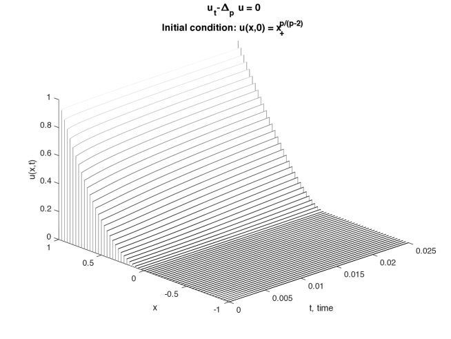
Figure 2. Waterfall plot of the numerical solution of 9.7, $p=4$, observe the difference in profile at beginning and end.

Since we are interested in the support of our numerical solution, we will consider the equation satisfied by the interface ($u\equiv 0$), actually we will be considering the equation of a basic level set. That is, we are looking for a curve $\gamma:{\mathbb{R}}_{+}\to{\mathbb{R}}$ such that for a given level $M\geq 0$ the following holds

$$u(\gamma(t),t)=M.$$

We will be considering the above problem with the initial point $\gamma(0)$ be be a point in the initial data that is equal to $M$, and for $M=0$ it will be the edge of the support, i.e. $x=0$. Proceeding formally and differentiating, the condition for $\gamma$ gives us,

$$u_{x}\gamma^{\prime}+u_{t}=0,$$ (9.8)

which after inserting the equation 2.1 into 9.8 yields

$$-\gamma^{\prime}(t)=\frac{\Delta_{p}u}{u_{x}}(\gamma(t),t)=(p-1)(u_{x}(\gamma(t),t))^{p-3}u_{xx}(\gamma(t),t).$$

In Fig. 3 we see the result of the above equation when using the numerical solution of 9.7 seen in Fig. 2 as the approximate values for $u$ and approximating the first and second derivative with the respective FD quotients, as described in 9.7.

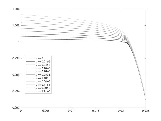
Figure 3. Level sets, conjectured critical time is $t\approx 0.0208$, $p=4$.

Upon visual inspection of Fig. 3 we see the sharp deviation of the support after roughly $t=0.02$, which coincides quite well with the conjectured value of $0.0208$ for $p=4$.

Based upon heuristic ideas we can expect that the profile of the solution towards the edge of the support will after the critical time behave like the Barenblatt solution, i.e. $u(x)\approx d(x,S(t)^{C})^{\frac{p-1}{p-2}}$, where $S(t)$ is the support of the solution at $t$. The numerical result of the behavior at $1.2\hat{t}$ can be found in Fig. 4 and the coincidence is striking, the edge of the support is estimated using the solution in Fig. 3.

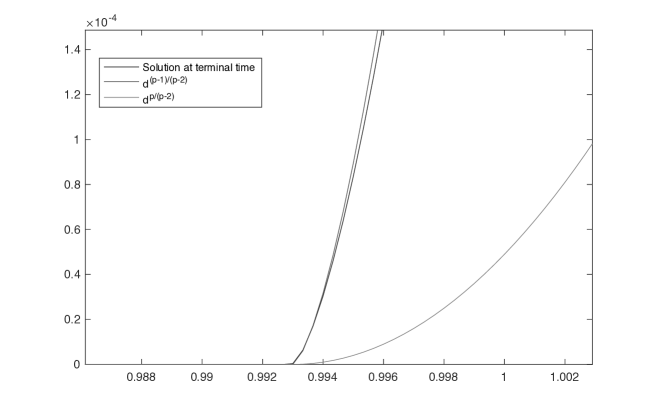
Figure 4. Plot of the numerical solution of 9.7, $p=4$ at time $1.2\hat{t}$, observe the coincidence of the profile of the solution with the profile of the Barenblatt, as compared to the profile of the initial datum (shifted to become zero at the same point as the other functions).

References

- [1] B. Avelin, On time dependent domains for the degenerate -parabolic equation: Carleson estimate and Hölder continuity, Math. Ann. 364(1) (2016), 667–686.
- [2] B. Avelin, U. Gianazza and S. Salsa, Boundary estimates for certain degenerate and singular parabolic equations, J. Eur. Math. Soc., 18(2) (2016), 381–426.
-
[3]
B. Avelin, T. Kuusi and K. Nyström, Boundary behavior of solutions to the
parabolic -Laplace equation, Anal. PDE, 12(1) (2019), 1–-42. - [4] A. Björn, J. Björn and U. Gianazza, The Petrovskiĭ criterion and barriers for degenerate and singular p-parabolic equations, U. Math. Ann, 368(3–4) (2017), 885–904.
- [5] A. Björn, J. Björn, U. Gianazza and M. Parviainen, Boundary regularity for degenerate and singular parabolic equations, Calc. Var. Partial Differential Equations 52(3) (2015), 797–827.
- [6] E. DiBenedetto, Degenerate parabolic equations, Springer Verlag, Series Universitext, New York, (1993).
- [7] U. Gianazza, N. Liao and T. Lukkari, A Boundary Estimate for Singular Parabolic Diffusion Equations, NoDEA Nonlinear Differential Equations Appl. 25(4) (2018).
- [8] U. Gianazza and S. Salsa, On the boundary behaviour of solutions to parabolic equations of −Laplacian type, Rend. Istit. Mat. Univ. Trieste 48 (2016), 463–-483.
- [9] D. Jerison and C. Kenig, Boundary behavior of harmonic functions in non-tangentially accessible domains, Adv. Math. 46 (1982), 80–147.
- [10] N. Ju, Numerical Analysis of Parabolic p-Laplacian: Approximation of Trajectories, SIAM Journal on Numerical Analysis 37(6) (2000), 1861–1884.
- [11] T. Kilpeläinen and P. Lindqvist, On the Dirichlet boundary value problem for a degenerate parabolic equation., SIAM J. Math. Anal. 27(3) (1996), 661–683.
- [12] T. Kuusi, G. Mingione and K. Nyström, A boundary Harnack inequality for singular equations of -parabolic type. Proc. Amer. Math. Soc. 142(8) (2014), 2705–2719.
- [13] J. Lewis and K. Nyström, Boundary behavior for -harmonic functions in Lipschitz and starlike Lipschitz ring domains. Ann. Sci. École Norm. Sup. (4) 40(5) (2007), 765–813.
- [14] J. Lewis and K. Nyström, Boundary behavior and the Martin boundary problem for -harmonic functions in Lipschitz domains. Ann. of Math. (2) 172(3) (2010), 1907–1948.
- [15] J.L. Vázquez, The porous medium equation. Mathematical theory. Oxford Mathematical Monographs. The Clarendon Press, Oxford University Press, Oxford, 2007. xxii+624 pp.