New inertial algorithm for a class of equilibrium problems

Abstract

The article introduces a new algorithm for solving a class of equilibrium problems involving strongly pseudomonotone bifunctions with a Lipschitz-type condition. We describe how to incorporate the proximal-like regularized technique with inertial effects. The main novelty of the algorithm is that it can be done without previously knowing the information on the strongly pseudomonotone and Lipschitz-type constants of cost bifunction. A reasonable explain for this is that the algorithm uses a sequence of stepsizes which is diminishing and non-summable. Theorem of strong convergence is proved. In the case, when the information on the modulus of strong pseudomonotonicity and Lispchitz-type constant is known, the rate of linear convergence of the algorithm has been established. Several of experiments are performed to illustrate the numerical behavior of the algorithm and also compare it with other algorithms.

1 Introduction

The equilibrium problem (briefly, EP) BO1994 ; MO1992 is well known as the Ky Fan inequality early studied in F1972 ; NI55 . Mathematically, problem (EP) can be considered as a generalization of many mathematical models such as variational inequality problems, optimization problems, fixed point problems, complementarity problems and Nash equilibrium problems, see, e.g., BO1994 ; FP2002 ; K2007 ; MO1992 . So, problem (EP) becomes an attractive field in mathematics as well as in applied sciences. In recent years, problem (EP) has been widely studied in both theoretically and algorithmically. Some methods for solving problem (EP) can be found, for instance, in A2013 ; A1995 ; BCCP13 ; BCP09 ; CH2005 ; FA1997 ; HMA2016 ; H2017COAP ; H2016c ; H2016e ; H2017 ; H2016 ; K2003 ; K2007 ; M2000 ; M2003 ; M1999 ; MQ2009 ; QMH2008 ; SS2011 ; SNN2013 . One of the most popular methods for solving problem (EP) is the proximal point method (PPM). This method was first introduced by Martinet M1970 for monotone variational inequality problems and after that it was extended by Rockafellar R1976 to monotone operators. Moudafi M1999 extended further the PPM to EPs for monotone bifunctions. In K2003 , Konnov also introduced another version of the PPM with weaker assumptions.
Another notable class of solution methods for solving problem (EP) is given by the so-called descent methods KA2006 ; KP2003 . They are based on the reformulation of the problem (EP) as a global optimization problem through the gap function or D-gap function and the regularization technique. The computations in these approaches often consist of evaluating the gap function at a point and searching the optimization direction based on the exact solution of a convex optimization problem. In recent years, the descent-like methods have been widely and intensively investigated under various types of weaker assumptions imposed on feasible set and cost bifunction, and also to reduce the computational complexity of algorithms, see, e.g., BP2015 ; BP2012 ; C2013 ; DPS2014 .
Now, we are interested in a method, which is based on the auxiliary problem principle, was early introduced in FA1997 and its convergence was also studied. Recently, the authors in QMH2008 have further extended and investigated the convergence of it under different assumptions that equilibrium bifunctions are pseudomonotone and satisfy a certain Lipschitz-type condition M2000 . The method in FA1997 ; QMH2008 was also called the extragradient method due to the results of Korpelevich K1976 on saddle point problems. Another similar method, which is called the two-step proximal method, has been recently considered by the authors in LS2016 . The main advantage of this method is that it only requires to proceed a value of bifunction at the current approximation. Its convergence was also established under the hypotheses of pseudomonotonicity and Lipschitz-type condition of bifunctions. In recent years, many iterative methods based on the extragradient-like methods have been proposed for solving problem (EP) under various types of conditions, see, for instance HMA2016 ; H2016c ; H2016e ; LS2016 ; SVN2015 and the references therein.
It is emphasized here that the aforementioned extragradient-like methods often use stepsizes which depend on Lipschitz-type constants of equilibrium bifunctions. This means that the Lipschitz-type constants must be the input parameters of used method, and so the prior knowledge of these constants is a requirement in actual fact for constructing sequences of solution approximations. That fact can make some restrictions in applications because the Lipschitz-type constants are often unknown or difficult to approximate. Very recently, the works H2017AA ; H2017NUMA have introduced the two extragradient-like methods (with two proximal-like steps over iteration) for solving strongly pseudomonotone and Lipschitz-type equilibrium problems where their main advantage is that they can be done without the prior knowledge of Lipschitz-type constants and of the modulus of strong pseudomonotonicity.
In this paper, we introduce continuously a new algorithm for solving problem (EP) involving strongly pseudomonotone bifunctions with a Lipschitz-type condition. As in H2017AA ; H2017NUMA , the new algorithm also can be performed in the case the information on strongly pseudomonotone and Lipschitz-type constant is unknown. This comes from a fact that the algorithm has used a variable sequence of stepsizes which is diminishing and non-summable. A theorem of strong convergence is proved. In the case, when the modulus of strong pseudomonotonicity and Lipschitz-type constants of cost bifunction are known, the rate of linear convergence of the algorithm is established. A notable difference in comparison with the extragradient-like methods in H2017AA ; H2017NUMA is that the proposed algorithm only uses a proximal-like regularized step per each iteration. In addition, the regularized step in the algorithm has been combined with inertial effects which has been studied recently by several authors, see, for instance, in AA2001 ; A2004 ; BCL2016 ; MM2008 ; Mo2003 and the references therein. As the results in AA2001 ; A2004 ; BCL2016 ; MM2008 ; Mo2003 , the extrapolation inertial term is intended to speed up the convergence properties. The main advantages of the new algorithm in this paper have been also confirmed by several numerical results.
The remainder of this paper is organized as follows: In Sect. 2 we recall some definitions and preliminary results used in the paper. Sect. 3 introduces in details the inertial regularized algorithm and gives an estimate on the sequence generated by the algorithm. Sect. 4 analyzes the convergence of the algorithm in the case the strongly pseudomonotone and Lipschitz-type constants are unknown. When these constants are known, we will establishe the rate of linear convergence of the algorithm in Sect. 5. Finally, in Sect. 6 we compare the numerical behavior of the new algorithm with the regularized algorithm (without inertial effect) and the extragradient-like ones having the same features proposed in H2017AA ; H2017NUMA .

2 Preliminaries

The paper concerns about solving an equilibrium problem in a real Hilbert space $H$. Let $C$ be a nonempty closed convex subset of $H$ and let $f$ be a bifunction from $H\times H$ to the set of real numbers $\Re$ such that $f(x,x)=0$ for all $x\in C$. Recall that the equilibrium problem (EP) for the bifunction $f$ on $C$ is to find $x^{*}\in C$ such that

$$f(x^{*},y)\geq 0,~{}\forall y\in C.$$

Solution methods for solving problem (EP) are often relative to theory of monotonicity of an operator or a bifunction. Now, we recall some concepts of monotonicity of a bifunction, see BO1994 ; MO1992 for more details. A bifunction $f:H\times H\to\Re$ is called:
(i) strongly monotone on $C$ if there exists a constant $\gamma>0$ such that

$$f(x,y)+f(y,x)\leq-\gamma||x-y||^{2},~{}\forall x,y\in C;$$

(ii) monotone on $C$ if

$$f(x,y)+f(y,x)\leq 0,~{}\forall x,y\in C;$$

(iii) pseudomonotone on $C$ if

$$f(x,y)\geq 0\Longrightarrow f(y,x)\leq 0,~{}\forall x,y\in C;$$

(iv) strongly pseudomonotone on $C$ if there exists a constant $\gamma>0$ such that

$$f(x,y)\geq 0\Longrightarrow f(y,x)\leq-\gamma||x-y||^{2},~{}\forall x,y\in C.$$

It is easy to see from the aforementioned definitions that the following implications hold,

$${\rm(i)}\Longrightarrow{\rm(ii)}\Longrightarrow{\rm(iii)}~{}{\rm and}~{}{\rm(i)}\Longrightarrow{\rm(iv)}\Longrightarrow{\rm(iii)}.$$

The converses in general are not true. We say that a bifunction $f:H\times H\to\Re$ satisfies Lipschitz-type condition if there exists a real number $L>0$ such that

$$f(x,y)+f(y,z)\geq f(x,z)-L||x-y||||y-z||,~{}\forall x,y,z\in H.$$

Note that if $A:H\to H$ is a Lipschitz continuous operator, i.e., there exists $L>0$ such that $||Ax-Ay||\leq L||x-y||$ for all $x,y\in H$, then the bifunction $f(x,y)=\left\langle Ax,y-x\right\rangle$ satisfies the Lipschitz-type condition (LC) with the constant $L$. Indeed, we have that $f(x,y)+f(y,z)-f(x,z)=\left\langle Ay-Ax,y-z\right\rangle\geq-||Ay-Ax||||y-z||\geq-L||y-x||||y-z||$. Thus, condition (LC) holds for $f$.

Remark 2.1

The Lipschitz-type condition (LC) implies the following condition which is called the Lipschitz-type condition in the sense of Mastroeni M2000 ,

$$f(x,y)+f(y,z)\geq f(x,z)-c_{1}||x-y||^{2}-c_{2}||y-z||^{2},~{}\forall x,y,z\in H,$$

where $c_{1}>0,~{}c_{2}>0$ are two given constants. Indeed, if condition (LC) holds then by the following relation

$$\left(\sqrt{\frac{L}{2\mu}}||x-y||-\sqrt{\frac{L\mu}{2}}||y-z||\right)^{2}\geq 0,$$

we have

$$f(x,y)+f(y,z)\geq f(x,z)-L||x-y||||y-z||\geq f(x,z)-\frac{L}{2\mu}||x-y||^{2}-\frac{L\mu}{2}||y-z||^{2}$$

for any $\mu>0$. This means that the Lipschitz-type condition of Mastroeni (MLC) in M2000 holds for the bifunction $f$ with $c_{1}=\frac{L}{2\mu}$ and $c_{2}=\frac{L\mu}{2}$.

Throughout this paper, for solving problem (EP), we assume that bifunction $f:H\times H\to\Re$ satisfies the following conditions:
(A1) $f(x,x)=0$ for all $x\in C$;
(A2) $f$ is strongly pseudomonotone on $C$ with some constant $\gamma$;
(A3) $f$ satisfies the Lipschitz-type condition (LC) on $H$ with some constant $L$;
(A4) $f(x,.)$ is convex and lower semicontinuous and $f(.,y)$ is hemicontinuous on $C$.
Note that, under hypotheses (A2) and (A4), problem (EP) has an unique solution, denoted by $x^{*}$. The Lipschitz-type conditions are often used in establishing the convergence of extragradient-like methods for EPs, see, e.g., HMA2016 ; H2016c ; H2016e ; LS2016 ; QMH2008 ; SVN2015 . Recall that a function $h:C\to\Re$ is called hemicontinuous on $C$ if $\lim\limits_{t\to 0}h(tz+(1-t)x)=h(x)$ for all $x,~{}z\in C$. The proximal mapping of a proper, convex and lower semicontinuous function $g:C\to\Re$ with a parameter $\lambda>0$ is defined by

$${\rm prox}_{\lambda g}(x)=\arg\min\left\{\lambda g(y)+\frac{1}{2}||x-y||^{2}:y\in C\right\},~{}x\in H.$$

The following is a property of the proximal mapping, see BC2011 for more details.

Lemma 2.1

For all $x\in H,~{}y\in C$ and $\lambda>0$, the following inequality holds,

$$\lambda\left\{g(y)-g({\rm prox}_{\lambda g}(x))\right\}\geq\left\langle x-{\rm prox}_{\lambda g}(x),y-{\rm prox}_{\lambda g}(x)\right\rangle.$$

Remark 2.2

From Lemma 2.1, it is easy to show that if $x={\rm prox}_{\lambda g}(x)$ then

$$x\in{\rm arg}\min\left\{g(y):y\in C\right\}:=\left\{x\in C:g(x)=\min_{y\in C}g(y)\right\}.$$

The following technical lemma will be used to prove theorem of convergence in Sect. 4.

Lemma 2.2

AA2001 Let $\{\Phi_{n}\}$, $\{\Delta_{n}\}$ and $\{\theta_{n}\}$ be sequences in $[0,+\infty)$ such that

$$\Phi_{n+1}\leq\Phi_{n}+\theta_{n}(\Phi_{n}-\Phi_{n-1})+\Delta_{n},~{}\forall n\geq 1,\quad\sum_{n=1}^{+\infty}\Delta_{n}<+\infty,$$

and there exists a real number $\theta$ with $0\leq\theta_{n}\leq\theta<1$ for all $n\geq 0$. Then the followings hold:
(i) $\sum_{n=1}^{+\infty}[\Phi_{n}-\Phi_{n-1}]_{+}<+\infty$, where $[t]_{+}:=\max\{t,0\}$;
(ii) There exists $\Phi_{*}\in[0,+\infty)$ such that $\lim_{n\to+\infty}\Phi_{n}=\Phi_{*}.$

Finally, in any Hilbert space, we have the following result, see, e.g., in (BC2011, , Corollary 2.14).

Lemma 2.3

For all $x,~{}y\in H$ and $\alpha\in\Re$, the following equality always holds

$$\|\alpha x+(1-\alpha)y\|^{2}=\alpha\|x\|^{2}+(1-\alpha)\|y\|^{2}-\alpha(1-\alpha)\|x-y\|^{2}.$$

3 Inertial regularized algorithm

This section introduces a new algorithm for solving problem (EP) involving strongly pseudomonotone and Lipschitz-type bifunctions. The algorithm can be considered as a combination of the proximal-like regularized technique and inertial effect. The following is the algorithm in details.
 

Algorithm 3.1 (Inertial Regularized Algorithm - IRA)

.
 
Initialization: Choose $x_{0},~{}x_{1}\in C$ and two sequences $\left\{\lambda_{n}\right\}\subset(0,+\infty)$ and $\left\{\theta_{n}\right\}\subset[0,1]$.
 
Iterative Steps: Assume that $x_{n-1},~{}x_{n}\in C$ are known, calculate $x_{n+1}$ as follows:

Step 1. Set $w_{n}=x_{n}+\theta_{n}(x_{n}-x_{n-1})$ and compute for each $n\geq 1$,

$$x_{n+1}={\rm prox}_{\lambda_{n}f(w_{n},.)}(w_{n}).$$

Step 2. If $x_{n+1}=w_{n}$ then stop and $x_{n+1}$ is the solution of problem (EP).

Otherwise, set $n:=n+1$ and go back Step 1.

 

Remark 3.3

The main task of Algorithm 3.1 is to compute the proximal mapping in Step 1. This can be equivalently rewritten as

$$x_{n+1}=\arg\min\left\{\lambda_{n}f(w_{n},y)+\frac{1}{2}||w_{n}-y||^{2}:y\in C\right\}.$$

Under hypotheses (A1) and (A4), from Lemma 2.1 and Remark 2.2, it is easy to see that if Algorithm 3.1 terminates at some iterate $n$, i.e., $x_{n+1}=w_{n}$ then $x_{n+1}$ is the solution of problem (EP). Throughout the paper, we assume that Algorithm 3.1 does not stop. This means that the sequence $\left\{x_{n}\right\}$ generated by Algorithm 3.1 is infinite. When $\theta_{n}=0$, Algorithm 3.1 can give us a regularized algorithm with a proximal-like step. As in AA2001 ; A2004 ; BCL2016 ; MM2008 ; Mo2003 , when $\theta_{n}\neq 0$, the extrapolation term $\theta_{n}(x_{n}-x_{n-1})$ is called the inertial effect and intended to speed up the convergence properties. This is also illustrated in our numerical experiments in the final part of this paper.

Also, under hypotheses (A2) and (A4), problem (EP) has an unique solution. This unique solution will be denoted by $x^{*}$ in what follows. The following lemma will be used repeatedly in the next two sections.

Lemma 3.4

Suppose that assumptions (A1) - (A4) hold. Then, the sequence $\left\{x_{n}\right\}$ generated by Algorithm 3.1 satisfies the following estimate,

$$(1+\lambda_{n}(2\gamma-L\sqrt{\lambda_{n}}))||x_{n+1}-x^{*}||^{2} \leq (1+\theta_{n})||x_{n}-x^{*}||^{2}-\theta_{n}||x_{n-1}-x^{*}||^{2}$$

$$-M_{n}||x_{n+1}-x_{n}||^{2}+N_{n}||x_{n}-x_{n-1}||^{2},$$

where

$$M_{n}=(1-\theta_{n})(1-L\sqrt{\lambda_{n}}),~{}N_{n}=\theta_{n}\left[1+\theta_{n}+(1-\theta_{n})(1-L\sqrt{\lambda_{n}})\right].$$

Proof

From the definitions of the proximal mapping and of $x_{n+1}$, we can write

$$x_{n+1}={\rm prox}_{\lambda_{n}f(w_{n},.)}(w_{n})=\arg\min\left\{f_{n}(x):x\in C\right\},$$ (1)

where $f_{n}(x)=\lambda_{n}f(w_{n},x)+\frac{1}{2}||x-w_{n}||^{2}$. From relation (1) and using the optimality condition, we obtain $0\in\partial f_{n}(x_{n+1})+N_{C}(x_{n+1})$. Thus, there exists $g^{*}_{n}\in\partial f_{n}(x_{n+1})$ such that $-g_{n}^{*}\in N_{C}(x_{n+1})$, i.e.,

$$\left\langle g^{*}_{n},x-x_{n+1}\right\rangle\geq 0,~{}\forall x\in C.$$ (2)

Since $f(w_{n},.)$ is convex, $f_{n}(x)$ is strongly convex with the modulus $1$. This implies that

$$f_{n}(x_{n+1})+\left\langle g_{n},x-x_{n+1}\right\rangle+\frac{1}{2}||x-x_{n+1}||^{2}\leq f_{n}(x),~{}\forall x\in C,$$ (3)

for any $g_{n}\in\partial f_{n}(x_{n+1})$. Substituting $g_{n}=g_{n}^{*}$ and $x=x^{*}$ into relation (3) and using relation (2), we get

$$f_{n}(x_{n+1})+\frac{1}{2}||x^{*}-x_{n+1}||^{2}\leq f_{n}(x^{*}),$$

which together with the definition of $f_{n}$ implies that

$$||x_{n+1}-x^{*}||^{2}\leq 2\lambda_{n}\left\{f(w_{n},x^{*})-f(w_{n},x_{n+1})\right\}+||w_{n}-x^{*}||^{2}-||x_{n+1}-w_{n}||^{2}.$$ (4)

Using the Lipschitz-type condition of $f$ and the Cauchy inequality, we obtain that

$$f(w_{n},x^{*})-f(w_{n},x_{n+1})\leq f(x_{n+1},x^{*})+L||x_{n+1}-w_{n}||||x_{n+1}-x^{*}||$$ (5)

$$\leq f(x_{n+1},x^{*})+\frac{L}{2}\left(\frac{1}{\sqrt{\lambda_{n}}}||x_{n+1}-w_{n}||^{2}+\sqrt{\lambda_{n}}||x_{n+1}-x^{*}||^{2}\right).$$

Since $x^{*}$ is the solution of problem (EP), $f(x^{*},x_{n+1})\geq 0$. Thus, from the strong pseudomotonicity of $f$, we obtain that $f(x_{n+1},x^{*})\leq-\gamma||x_{n+1}-x^{*}||^{2}$. This together with relation (5) implies that

$$f(w_{n},x^{*})-f(w_{n},x_{n+1})\leq-(\gamma-\frac{L\sqrt{\lambda_{n}}}{2})||x_{n+1}-x^{*}||^{2}+\frac{L}{2\sqrt{\lambda_{n}}}||x_{n+1}-w_{n}||^{2}.$$

Multiplying both two sides of the last inequality by $2\lambda_{n}$, we obtain

$$2\lambda_{n}\left(f(w_{n},x^{*})-f(w_{n},x_{n+1})\right) \leq -\lambda_{n}(2\gamma-L\sqrt{\lambda_{n}})||x_{n+1}-x^{*}||^{2}$$ (6)

$$+L\sqrt{\lambda_{n}}||x_{n+1}-w_{n}||^{2}.$$

It follows from relations (4) and (6) that

$$(1+\lambda_{n}(2\gamma-L\sqrt{\lambda_{n}}))||x_{n+1}-x^{*}||^{2}\leq||w_{n}-x^{*}||^{2}-(1-L\sqrt{\lambda_{n}})||x_{n+1}-w_{n}||^{2}.$$ (7)

From the definition of $w_{n}$ and Lemma 2.3 we have

$$||w_{n}-x^{*}||^{2} = ||(1+\theta_{n})(x_{n}-x^{*})-\theta_{n}(x_{n-1}-x^{*})||^{2}$$ (8)

$$= (1+\theta_{n})||x_{n}-x^{*}||^{2}-\theta_{n}||x_{n-1}-x^{*}||^{2}$$

$$+\theta_{n}(1+\theta_{n})||x_{n}-x_{n-1}||^{2}.$$

It also follows from the definition of $w_{n}$ that

$$||x_{n+1}-w_{n}||^{2}=||x_{n+1}-x_{n}-\theta_{n}(x_{n}-x_{n-1})||^{2}$$ (9)

$$= ||x_{n+1}-x_{n}||^{2}+\theta^{2}_{n}||x_{n}-x_{n-1}||^{2}-2\theta_{n}\left\langle x_{n+1}-x_{n},x_{n}-x_{n-1}\right\rangle$$

$$\geq ||x_{n+1}-x_{n}||^{2}+\theta^{2}_{n}||x_{n}-x_{n-1}||^{2}-2\theta_{n}||x_{n+1}-x_{n}||||x_{n}-x_{n-1}||$$

$$\geq ||x_{n+1}-x_{n}||^{2}+\theta^{2}_{n}||x_{n}-x_{n-1}||^{2}-\theta_{n}\left[||x_{n+1}-x_{n}||^{2}+||x_{n}-x_{n-1}||^{2}\right]$$

$$= (1-\theta_{n})||x_{n+1}-x_{n}||^{2}-\theta_{n}(1-\theta_{n})||x_{n}-x_{n-1}||^{2}.$$

Combining relations (7), (8) and (9), we get

$$(1+\lambda_{n}(2\gamma-L\sqrt{\lambda_{n}}))||x_{n+1}-x^{*}||^{2}\leq(1+\theta_{n})||x_{n}-x^{*}||^{2}-\theta_{n}||x_{n-1}-x^{*}||^{2}$$

$$-(1-\theta_{n})(1-L\sqrt{\lambda_{n}})||x_{n+1}-x_{n}||^{2}$$

$$+\theta_{n}\left[1+\theta_{n}+(1-\theta_{n})(1-L\sqrt{\lambda_{n}})\right]||x_{n}-x_{n-1}||^{2},$$

which together with the definitions of $M_{n}$, $N_{n}$ implies the desired conclusion. Lemma 3.4 is proved.

Remark 3.4

In the case, when $f$ satisfies the condition (MLC) of Mastroeni in M2000 with two constants $c_{1}$ and $c_{2}$ then we have the following estimate

$$(1+2\lambda_{n}(\gamma-c_{2}))||x_{n+1}-x^{*}||^{2} \leq (1+\theta_{n})||x_{n}-x^{*}||^{2}-\theta_{n}||x_{n-1}-x^{*}||^{2}$$ (10)

$$-\bar{M}_{n}||x_{n+1}-x_{n}||^{2}+\bar{N}_{n}||x_{n}-x_{n-1}||^{2},$$

where $\bar{M}_{n}=(1-\theta_{n})(1-2\lambda_{n}c_{1}),~{}\bar{N}_{n}=\theta_{n}\left[1+\theta_{n}+(1-\theta_{n})(1-2\lambda_{n}c_{1})\right].$ Indeed, from relation (4) and the condition (MLC) of $f$ that

$$f(w_{n},x^{*})-f(w_{n},x_{n+1})\leq f(x_{n+1},x^{*})+c_{1}||x_{n+1}-w_{n}||^{2}+c_{2}||x_{n+1}-x^{*}||^{2},$$

we obtain

$$||x_{n+1}-x^{*}||^{2} \leq 2\lambda_{n}\left[f(x_{n+1},x^{*})+c_{1}||x_{n+1}-w_{n}||^{2}+c_{2}||x_{n+1}-x^{*}||^{2}\right]$$

$$+||w_{n}-x^{*}||^{2}-||x_{n+1}-w_{n}||^{2}.$$

This together with the fact $f(x_{n+1},x^{*})\leq-\gamma||x_{n+1}-x^{*}||^{2}$ implies that

$$||x_{n+1}-x^{*}||^{2} \leq 2\lambda_{n}\left[-\gamma||x_{n+1}-x^{*}||^{2}+c_{1}||x_{n+1}-w_{n}||^{2}+c_{2}||x_{n+1}-x^{*}||^{2}\right]$$

$$+||w_{n}-x^{*}||^{2}-||x_{n+1}-w_{n}||^{2}.$$

Thus

$$(1+2\lambda_{n}(\gamma-c_{2}))||x_{n+1}-x^{*}||^{2}\leq||w_{n}-x^{*}||^{2}-(1-2\lambda_{n}c_{1})||x_{n+1}-w_{n}||^{2}.$$ (11)

It follows from relations (8), (9) and (11) that

$$(1+2\lambda_{n}(\gamma-c_{2}))||x_{n+1}-x^{*}||^{2} \leq (1+\theta_{n})||w_{n}-x^{*}||^{2}-\theta_{n}||x_{n+1}-w_{n}||^{2}$$

$$-(1-\theta_{n})(1-2\lambda_{n}c_{1})||x_{n+1}-x_{n}||^{2}$$

$$+\theta_{n}\left[1+\theta_{n}+(1-\theta_{n})(1-2\lambda_{n}c_{1})\right]||x_{n}-x_{n-1}||^{2},$$

which, from the definitons of $\bar{M}_{n}$ and $\bar{N}_{n}$, is equivalent to relation (10).

4 Inertial regularized algorithm without prior constants

In this section, we consider Algorithm 3.1 for solving problem (EP) for a bifunction $f$ which is strongly pseudomonotone with some modulus $\gamma$ (hypothesis (A2)) and satisfies the Lipschitz-type condition (LC) with some constant $L$ (hypothesis (A3)). However, as in H2017AA ; H2017NUMA , we will establish that Algorithm 3.1 can be done without the prior knowledge of the constants $\gamma$ and $L$. This is particularly interesting when those constants are unknown or difficult to approximate. In order to get that result, in Algorithm 3.1 we consider the sequence of stepsizes $\left\{\lambda_{n}\right\}\subset(0,+\infty)$ and the sequence of inertial parameters $\left\{\theta_{n}\right\}\subset[0,1]$ satisfying the following conditions:
(H1): $\lim_{n\to\infty}\lambda_{n}=0,\qquad{\rm(H2)}:\sum_{n=0}^{\infty}\lambda_{n}=+\infty.$
(H3): $\left\{\theta_{n}\right\}$ is non-decreasing and $\theta_{n}\in[0,\theta_{*}]$ for some $\theta_{*}\in[0,\frac{1}{3})$.
A simple example of sequence $\left\{\lambda_{n}\right\}$ satisfies conditions (H1) and (H2) as $\lambda_{n}=\frac{1}{(n+1)^{p}}$ for each $n\geq 0$, where $p\in(0,1]$. We have the following first main result.

Theorem 4.1

Under hypotheses (A1) - (A4) and (H1) - (H3), then the sequence $\left\{x_{n}\right\}$ generated by Algorithm 3.1 converges strongly to the unique solution $x^{*}$ of problem (EP).

Proof

Since $0\leq\theta^{*}<\frac{1}{3}$, we obtain $0\leq\frac{2\theta^{*}}{1-\theta^{*}}<1$. Now let $\sigma$ be fixed in the interval $(\frac{2\theta_{*}}{1-\theta_{*}},1)$. Since $\lambda_{n}\to 0$, there exists $n_{0}\geq 0$ such that for all $n\geq n_{0}$,

$$1-L\sqrt{\lambda_{n}}\geq\sigma~{}\mbox{and}~{}2\gamma-L\sqrt{\lambda_{n}}\geq\gamma>0.$$ (12)

It follows from Lemma 3.4 and relation (12) that, for all $n\geq n_{0},$

$$||x_{n+1}-x^{*}||^{2} \leq (1+\lambda_{n}(2\gamma-L\sqrt{\lambda_{n}}))||x_{n+1}-x^{*}||^{2}$$ (13)

$$\leq (1+\theta_{n})||x_{n}-x^{*}||^{2}-\theta_{n}||x_{n-1}-x^{*}||^{2}$$

$$-M_{n}||x_{n+1}-x_{n}||^{2}+N_{n}||x_{n}-x_{n-1}||^{2}.$$

where $M_{n}$ and $N_{n}$ are recalled that

$$M_{n}=(1-\theta_{n})(1-L\sqrt{\lambda_{n}}),~{}N_{n}=\theta_{n}\left[1+\theta_{n}+(1-\theta_{n})(1-L\sqrt{\lambda_{n}})\right].$$ (14)

Let $\varphi_{n}=||x_{n}-x^{*}||^{2}-\theta_{n}||x_{n-1}-x^{*}||^{2}+N_{n}||x_{n}-x_{n-1}||^{2}$. Thus, from the non-decreasing property of $\left\{\theta_{n}\right\}$ and relation (13), we obtain that

$$\varphi_{n+1}-\varphi_{n} = ||x_{n+1}-x^{*}||^{2}-\theta_{n+1}||x_{n}-x^{*}||^{2}+N_{n+1}||x_{n+1}-x_{n}||^{2}$$ (15)

$$-||x_{n}-x^{*}||^{2}+\theta_{n}||x_{n-1}-x^{*}||^{2}-N_{n}||x_{n}-x_{n-1}||^{2}$$

$$\leq ||x_{n+1}-x^{*}||^{2}-(1+\theta_{n})||x_{n}-x^{*}||^{2}+N_{n+1}||x_{n+1}-x_{n}||^{2}$$

$$+\theta_{n}||x_{n-1}-x^{*}||^{2}-N_{n}||x_{n}-x_{n-1}||^{2}$$

$$\leq -M_{n}||x_{n+1}-x_{n}||^{2}+N_{n+1}||x_{n+1}-x_{n}||^{2}$$

$$= -(M_{n}-N_{n+1})||x_{n+1}-x_{n}||^{2}.$$

Moreover, from the definitions of $M_{n},~{}N_{n+1}$, relation (12), and the facts $\sigma\in(\frac{2\theta_{*}}{1-\theta_{*}},1)$ and $1-L\sqrt{\lambda_{n+1}}<1$ , we have for all $n\geq n_{0}$ that

$$M_{n}-N_{n+1} = (1-\theta_{n})(1-L\sqrt{\lambda_{n}})-\theta_{n+1}\left[1+\theta_{n+1}+(1-\theta_{n+1})(1-L\sqrt{\lambda_{n+1}})\right]$$

$$\geq (1-\theta_{n})\sigma-\theta_{n+1}\left[1+\theta_{n+1}+(1-\theta_{n+1})\right]$$

$$\geq (1-\theta_{n+1})\sigma-2\theta_{n+1}~{}\qquad\qquad(\mbox{since}~{}\theta_{n}\leq\theta_{n+1})$$

$$\geq (1-\theta_{*})\sigma-2\theta_{*}:=K>0.$$

This together with relation (15) implies that

$$\varphi_{n+1}-\varphi_{n}\leq-K||x_{n+1}-x_{n}||^{2},~{}\forall n\geq n_{0}.$$ (16)

Thus, $\left\{\varphi_{n}\right\}_{n=n_{0}}^{+\infty}$ is non-increasing. It follows from the definition of $\varphi_{n}$ that $\varphi_{n}\geq||x_{n}-x^{*}||^{2}-\theta_{n}||x_{n-1}-x^{*}||^{2}$, and thus, we obtain for all $n\geq n_{0}$ that

$$||x_{n}-x^{*}||^{2}\leq\varphi_{n}+\theta_{n}||x_{n-1}-x^{*}||^{2}\leq\varphi_{n_{0}}+\theta_{*}||x_{n-1}-x^{*}||^{2}.$$

Hence, we get by the induction that

$$||x_{n}-x^{*}||^{2}\leq\varphi_{n_{0}}(1+\theta_{*}+\ldots+\theta_{*}^{n-n_{0}})+\theta_{*}^{n-n_{0}}||x_{n_{0}}-x^{*}||^{2},~{}\forall n\geq n_{0},$$

which implies that

$$||x_{n}-x^{*}||^{2}\leq\frac{\varphi_{n_{0}}}{1-\theta_{*}}+\theta_{*}^{n-n_{0}}||x_{n_{0}}-x^{*}||^{2}.$$ (17)

It also follows from the definition of $\varphi_{n+1}$ that $\varphi_{n+1}\geq-\theta_{n+1}||x_{n}-x^{*}||^{2}$, and thus, from relation (17),

$$-\varphi_{n+1}\leq\theta_{n+1}||x_{n}-x^{*}||^{2}\leq\theta_{*}||x_{n}-x^{*}||^{2}\leq\frac{\theta_{*}\varphi_{n_{0}}}{1-\theta_{*}}+\theta_{*}^{n-n_{0}+1}||x_{n_{0}}-x^{*}||^{2}.$$ (18)

Thus, from relation (16), we obtain for all $N\geq n_{0}$ that

$$K\sum_{n=n_{0}}^{N}||x_{n+1}-x_{n}||^{2}\leq\varphi_{n_{0}}-\varphi_{N+1}\leq\frac{\varphi_{n_{0}}}{1-\theta_{*}}+\theta_{*}^{N-n_{0}+1}||x_{n_{0}}-x^{*}||^{2}.$$ (19)

Passing to the limit in the last inequality as $N\to\infty$ and nothing that $\theta_{*}\in[0,\frac{1}{3})$ and $K>0$, we obtain

$$\sum_{n=n_{0}}^{\infty}||x_{n+1}-x_{n}||^{2}<+\infty,$$ (20)

which implies that

$$\lim\limits_{n\to\infty}||x_{n+1}-x_{n}||^{2}=0.$$ (21)

It follows from relation (13) that

$$||x_{n+1}-x^{*}||^{2} \leq (1+\theta_{n})||x_{n}-x^{*}||^{2}-\theta_{n}||x_{n-1}-x^{*}||^{2}$$ (22)

$$+N_{n}||x_{n}-x_{n-1}||^{2}.$$

Let $\Phi_{n}=||x_{n}-x^{*}||^{2}$, $\Delta_{n}=N_{n}||x_{n}-x_{n-1}||^{2}$ and rewrite shortly inequality (22) as follows

$$\Phi_{n+1}\leq\Phi_{n}+\theta_{n}(\Phi_{n}-\Phi_{n-1})+\Delta_{n}.$$ (23)

Note that $\left\{N_{n}\right\}$ is bounded, and thus, from (20) we obtain that $\sum_{n=n_{0}}^{\infty}\Delta_{n}<+\infty$. This together with (23) and Lemma 2.2 implies that $\lim\limits_{n\to\infty}\Phi_{n}=\Phi_{*}\in\Re$, i.e.,

$$\lim\limits_{n\to\infty}||x_{n}-x^{*}||^{2}=\Phi_{*}\in\Re.$$ (24)

It follows from relations (7) and (12) that, for all $n\geq n_{0}$,

$$(1+\gamma\lambda_{n})||x_{n+1}-x^{*}||^{2}\leq(1+\lambda_{n}(2\gamma-L\sqrt{\lambda_{n}}))||x_{n+1}-x^{*}||^{2}\leq||w_{n}-x^{*}||^{2}$$

which, together with (8) and the non-decreasing property of $\left\{\theta_{n}\right\}$, implies that for each $n\geq n_{0}$,

$$\gamma\lambda_{n}||x_{n+1}-x^{*}||^{2}\leq-||x_{n+1}-x^{*}||^{2}+||w_{n}-x^{*}||^{2}$$

$$= -||x_{n+1}-x^{*}||^{2}+(1+\theta_{n})||x_{n}-x^{*}||^{2}-\theta_{n}||x_{n-1}-x^{*}||^{2}$$

$$+\theta_{n}(1+\theta_{n})||x_{n}-x_{n-1}||^{2}$$

$$= \left[||x_{n}-x^{*}||^{2}-||x_{n+1}-x^{*}||^{2}\right]+\left[\theta_{n}||x_{n}-x^{*}||^{2}-\theta_{n}||x_{n-1}-x^{*}||^{2}\right]$$

$$+\theta_{n}(1+\theta_{n})||x_{n}-x_{n-1}||^{2}$$

$$\leq \left[||x_{n}-x^{*}||^{2}-||x_{n+1}-x^{*}||^{2}\right]+\left[\theta_{n}||x_{n}-x^{*}||^{2}-\theta_{n-1}||x_{n-1}-x^{*}||^{2}\right]$$

$$+\theta_{*}(1+\theta_{*})||x_{n}-x_{n-1}||^{2}.$$

Let $N\geq n_{0}$ be fixed. Using the last inequality for $n=n_{0},n_{0}+1,\ldots,N$ and summing up these inequalities, we obtain that

$$\gamma\sum_{n=n_{0}}^{N}\lambda_{n}||x_{n+1}-x^{*}||^{2} \leq ||x_{n_{0}}-x^{*}||^{2}-||x_{N+1}-x^{*}||^{2}+\theta_{N}||x_{N}-x^{*}||^{2}$$

$$-\theta_{n_{0}-1}||x_{n_{0}-1}-x^{*}||^{2}+\theta_{*}(1+\theta_{*})\sum_{n=n_{0}}^{N}||x_{n}-x_{n-1}||^{2}.$$

Passing to the limit in the last inequality as $N\to\infty$ and using relattions (20), (24) and the boundedness of $\left\{\theta_{n}\right\}$, we obtain that

$$\sum_{n=1}^{\infty}\lambda_{n}||x_{n+1}-x^{*}||^{2}<+\infty,$$

which, together with hypothesis (H2), implies that $\lim\limits_{n\to\infty}\inf||x_{n+1}-x^{*}||^{2}=0$. In view of relation (24), we see that the limit of $\left\{||x_{n+1}-x^{*}||^{2}\right\}$ exists. Thus, $\lim\limits_{n\to\infty}||x_{n+1}-x^{*}||^{2}=0$ which completes the proof of Theorem 4.1.

Now, we consider several corollaries of Theorem 4.1. By choosing $\theta_{n}=0$, we obtain the following corollary.

Corollary 4.1

Suppose that hypotheses (A1) - (A4) and (H1) - (H2) hold. Let $\left\{x_{n}\right\}$ be a sequence generated by the following manner: choose $x_{0}\in C$ and for each $n\geq 0$, compute

$$x_{n+1}={\rm prox}_{\lambda_{n}f(x_{n},.)}(x_{n}).$$

Then, the sequence $\left\{x_{n}\right\}$ converges strongly to the unique solution $x^{*}$ of problem (EP).

Remark 4.5

In the case when $\theta_{n}=0$, we see that $N_{n}=0$, $M_{n}\geq 0$ and $2\gamma-L\sqrt{\lambda_{n}}\geq\gamma$ for all $n\geq n_{0}$. Thus, it follows from relation (13) that

$$(1+\gamma\lambda_{n})||x_{n+1}-x^{*}||^{2} < (1+\lambda_{n}(2\gamma-L\sqrt{\lambda_{n}}))||x_{n+1}-x^{*}||^{2}$$

$$\leq ||x_{n}-x^{*}||^{2},~{}\forall n\geq n_{0}.$$

This is equivalent to $||x_{n+1}-x^{*}||^{2}<\frac{1}{1+\gamma\lambda_{n}}||x_{n}-x^{*}||^{2}$. Thus, by the induction, we obtain for each $n\geq n_{0}$ that $||x_{n+1}-x^{*}||^{2}<\frac{1}{\prod_{i=n_{0}}^{n}(1+\gamma\lambda_{i})}||x_{n_{0}}-x^{*}||^{2}$. Hence, as in H2017AA , we come to the following estimate, for each $n\geq n_{0}$,

$$||x_{n+1}-x^{*}||^{2}<\frac{||x_{n_{0}}-x^{*}||^{2}}{1+\gamma\sum_{i=n_{0}}^{n}\lambda_{i}}.$$ (25)

Next, we consider a special case when problem (EP) is a variational inequality problem (VIP). Let $A:H\to H$ be a nonlinear operator. The problem (VIP) for an operator $A$ on $C$ is to find $x^{*}\in C$ such that

$$\left\langle Ax^{*},x-x^{*}\right\rangle\geq 0,~{}\forall x\in C.$$

Recall that an operator $A:C\to H$ is called: (i) Lipschitz continuous on $H$ if there exists a real number $L>0$ such that $||Ax-Ay||\leq L||x-y||$ for all $x,y\in H$; (ii) strongly pseudomonotone on $C$ if there exists a real number $\gamma>0$ such that the following implication holds,

$$\left\langle Ax,y-x\right\rangle\geq 0\Longrightarrow\left\langle Ay,x-y\right\rangle\leq-\gamma||x-y||^{2},~{}\forall x,y\in C.$$

Let $f(x,y)=\left\langle Ax,y-x\right\rangle$ for all $x,y\in H$. Then, ${\rm prox}_{\lambda f(x,.)}(x)=P_{C}(x-\lambda Ax)$ for all $x,y\in H$ and $\lambda>0$, and if $A$ is Lipschitz continuous and strongly pseudomonotone then assumptions (A1) - (A4) hold for $f$. Thus, the following corollary follows directly from Theorem 4.1.

Corollary 4.2

Suppose that $A:H\to H$ is a strongly pseudomonotone and Lipschitz continuous operator and $x^{*}$ is the unique solution of problem (VIP) for $A$ on $C$. Let $\left\{x_{n}\right\}$ be a sequences generated as follows: Choose $x_{0},~{}x_{1}\in C$ and for each $n$ compute $w_{n}=x_{n}+\theta_{n}(x_{n}-x_{n-1})$ and

$$x_{n+1}=P_{C}(w_{n}-\lambda_{n}Aw_{n}),$$

where $\left\{\lambda_{n}\right\}\subset(0,+\infty)$, $\left\{\theta_{n}\right\}\subset[0,1]$ are two sequences satisfying hypotheses (H1) - (H3). Then $\left\{x_{n}\right\}$ converges strongly to the unique solution $x^{*}$ of problem (VIP).

Remark 4.6

Algorithm 3.1 cannot converge linearly under hypotheses (H1) and (H2). Indeed, consider our problem for $f(x,y)=x(y-x)$ for all $x,y\in C=H=\Re$ and Algorithm 3.1 for $\theta_{n}=0$ and $\lambda_{n}\neq 1$ for all $n\geq 0$. The unique solution of the problem is $x^{*}=0$. From Algorithm 3.1 we obtain $x_{n+1}=(1-\lambda_{n})x_{n}$. Since $\lim\limits_{n\to\infty}\lambda_{n}=0$ and $x_{n}\neq 0$ for all $n\geq 0$, we have

$$\lim\limits_{n\to\infty}\frac{||x_{n+1}-x^{*}||}{||x_{n}-x^{*}||}=\lim\limits_{n\to\infty}|1-\lambda_{n}|=1.$$

Thus, we cannot find any real number $\alpha\in(0,1)$ such that $||x_{n+1}-x^{*}||\leq\alpha||x_{n}-x^{*}||$ for each $n\geq 0$. This says that Algorithm 3.1 cannot be linearly convergent. In the next section, we will establish the rate of linear convergence of Algorithm 3.1 when the strongly pseudomonotone and Lipschitz-type constants are known.

5 Inertial regularized algorithm with prior constants

This section also studies the convergence of Algorithm 3.1 under hypotheses (A2) and (A3). However, unlike the previous section, we consider the case when the modulus of strong pseudomonotonicity $\gamma$ and the Lipschitz-type constant $L$ are known. In that case, we establish the rate of linear convergence of Algorithm 3.1. For the sake of simplicity, in Algorithm 3.1, we consider that $\lambda_{n}=\lambda$, $\theta_{n}=\theta$ for all $n\geq 0$. In order to obtain the rate of convergence of the algorithm, we consider the following assumptions:
(H4) $0<\lambda<\min\left\{\frac{4\gamma^{2}}{L^{2}},\frac{1}{L^{2}}\right\}$.
(H5) $0\leq\theta<\min\left\{\lambda(2\gamma-L\sqrt{\lambda}),\frac{1-L\sqrt{\lambda}}{3-L\sqrt{\lambda}+2\lambda(2\gamma-L\sqrt{\lambda})}\right\}$.
We have the following second main result.

Theorem 5.1

Under hypotheses (A1) - (A4) and (H4) - (H5), then the sequence $\left\{x_{n}\right\}$ generated by Algorithm 3.1 converges linearly to the unique solution $x^{*}$ of problem (EP). Moreover, there exists $M>0$ such that for all $n\geq 1$,

$$||x_{n+1}-x^{*}||\leq M\alpha^{n},$$

where

$$\alpha=\sqrt{\frac{1+\theta}{1+\lambda(2\gamma-L\sqrt{\lambda})}}\in(0,1).$$

Proof

It follows from Lemma 3.4 with $\lambda_{n}=\lambda$, $\theta_{n}=\theta$ for all $n\geq 0$ that

$$(1+\lambda(2\gamma-L\sqrt{\lambda}))||x_{n+1}-x^{*}||^{2}+(1-\theta)(1-L\sqrt{\lambda})||x_{n+1}-x_{n}||^{2}$$

$$\leq(1+\theta)||x_{n}-x^{*}||^{2}+\theta\left[1+\theta+(1-\theta)(1-L\sqrt{\lambda})\right]||x_{n}-x_{n-1}||^{2}.$$

Dividing both two sides of the last inequality by $1+\lambda(2\gamma-L\sqrt{\lambda})>0$, we obtain that

$$||x_{n+1}-x^{*}||^{2}+B||x_{n+1}-x_{n}||^{2}\leq A||x_{n}-x^{*}||^{2}+C||x_{n}-x_{n-1}||^{2},$$ (26)

where

$$A=\frac{1+\theta}{1+\lambda(2\gamma-L\sqrt{\lambda})},~{}B=\frac{(1-\theta)(1-L\sqrt{\lambda})}{1+\lambda(2\gamma-L\sqrt{\lambda})},$$ (27)

$$C=\frac{\theta\left[1+\theta+(1-\theta)(1-L\sqrt{\lambda})\right]}{1+\lambda(2\gamma-L\sqrt{\lambda})}.$$ (28)

Under hypotheses (H4) - (H5), we see that $A>0$, $B>0$ and $C\geq 0$. Relation (26) can be rewritten as follows:

$$||x_{n+1}-x^{*}||^{2}+B||x_{n+1}-x_{n}||^{2} \leq A\left(||x_{n}-x^{*}||^{2}+B||x_{n}-x_{n-1}||^{2}\right)$$ (29)

$$-(AB-C)||x_{n}-x_{n-1}||^{2}.$$

Now, under hypothesis (H4) and (H5) we will imply that $AB\geq C$. Indeed, it follows from (H5) that $\theta(3-L\sqrt{\lambda}+2\lambda(2\gamma-L\sqrt{\lambda}))\leq 1-L\sqrt{\lambda}$. Thus, since $3-L\sqrt{\lambda}=(1-L\sqrt{\lambda})+2$, we obtain $2\theta(1+\lambda(2\gamma-L\sqrt{\lambda}))\leq(1-\theta)(1-L\sqrt{\lambda})$. This together with the fact $1-\theta\leq 1-\theta^{2}$ implies that $2\theta(1+\lambda(2\gamma-L\sqrt{\lambda}))\leq(1-\theta^{2})(1-L\sqrt{\lambda})=(1+\theta)(1-\theta)(1-L\sqrt{\lambda})$. Multiplying both two sides of this inequality by $\frac{1}{(1+\lambda(2\gamma-L\sqrt{\lambda}))^{2}}$, we come to the following estimate

$$\frac{(1+\theta)(1-\theta)(1-L\sqrt{\lambda})}{\left(1+\lambda(2\gamma-L\sqrt{\lambda})\right)^{2}}\geq\frac{2\theta}{1+\lambda(2\gamma-L\sqrt{\lambda})}.$$

Thus, since $2\theta=\theta\left[1+\theta+(1-\theta)\right]\geq\theta\left[1+\theta+(1-\theta)(1-L\sqrt{\lambda})\right]$, one has

$$\frac{(1+\theta)(1-\theta)(1-L\sqrt{\lambda})}{\left(1+\lambda(2\gamma-L\sqrt{\lambda})\right)^{2}}\geq\frac{\theta\left[1+\theta+(1-\theta)(1-L\sqrt{\lambda})\right]}{1+\lambda(2\gamma-L\sqrt{\lambda})}.$$

This together with the definitions of $A,~{}B,~{}C$ is equivalent to the inequality $AB\geq C$ or $AB-C\geq 0$. Thus, from relation (29), we obtain

$$||x_{n+1}-x^{*}||^{2}+B||x_{n+1}-x_{n}||^{2} \leq A\left(||x_{n}-x^{*}||^{2}+B||x_{n}-x_{n-1}||^{2}\right).$$

Therefore, we obtain by the induction that

$$||x_{n+1}-x^{*}||^{2}+B||x_{n+1}-x_{n}||^{2} \leq A^{n}\left(||x_{1}-x^{*}||^{2}+B||x_{1}-x_{0}||^{2}\right),~{}\forall n\geq 0.$$

Thus $||x_{n+1}-x^{*}||^{2}\leq A^{n}\left(||x_{1}-x^{*}||^{2}+B||x_{1}-x_{0}||^{2}\right)$, i.e.,

$$||x_{n+1}-x^{*}||\leq M\alpha^{n},$$

where $M=\sqrt{||x_{1}-x^{*}||^{2}+B||x_{1}-x_{0}||^{2}}$ and

$$\alpha=\sqrt{A}=\sqrt{\frac{1+\theta}{1+\lambda(2\gamma-L\sqrt{\lambda})}}.$$

Note that from hypothesis (H5) we obtain that $\alpha\in(0,1)$. Theorem 5.1 is proved.

Remark 5.7

In view of Remark 3.4 and the proofs of Theorem 4.1 and 5.1, we can establish the same convergence results for equilibrium problem (EP) with the Lipschitz-type condition (MLC) in M2000 under some suitable conditions imposed on stepsize as well as inertial parameter. It is worth mentioning that from the left-hand side of inequality (10), we always need the condition $\gamma>c_{2}$. This condition was also used in the regularized method, see, e.g., (MQ2009, , Corollary 2.1). We leave the proof in details to the readers.

6 Numerical illustrations

This section presents several experiments to illustrate the numerical behavior of the proposed algorithm - IRA (Algorithm 3.1) with different parameters, and also to compare with three other algorithms having the same features, namely the regularized algorithm - RA (see, Corollary 4.1), the extragradient method (EGM) presented in (H2017AA, , Algorithm 1) and the modified extragradient method (M-EGM) proposed in (H2017NUMA, , Algorithm 3.1). As in H2017AA ; H2017NUMA , the main advantage of Algorithm 3.1 is that it can be done without the prior knowledge of strongly pseudomonotone and Lipschitz-type constants of cost bifunction. This, as mentioned above, comes from the use of sequences of stepsizes being diminishing and non-summable. We use the following five sequences of stepsizes,

$$\lambda_{n}=\frac{1}{(n+1)^{p}},~{}p=1,~{}0.7,~{}0.5,~{}0.3,~{}0.1,$$

and five inertial parameters as $\theta_{n}\in\left\{0.1,~{}0.15,~{}0.2,~{}0.25,~{}0.3\right\}$. In the case, when the solution of the problem is unknown we use the function

$$D(x)=||x-\mbox{\rm prox}_{\lambda f(x,.)}(x)||^{2}$$

for some $\lambda>0$ to describe and compare the computational performance of all the algorithms. Note that if $D(x)=0$ then $x$ is the solution of the problem. Otherwise, if the solution $x^{*}$ of the problem is known, we use the function $E(x)=||x-x^{*}||^{2}$. All the programs are written in Matlab 7.0 and computed on a PC Desktop Intel(R) Core(TM) i5-3210M CPU @ 2.50GHz, RAM 2.00 GB.

6.1 Numerical behavior of Algorithm 3.1

This subsection studies the numerical behavior of Algorithm 3.1 on two test problems for different control parameters. The followings are the examples in details.
Example 1. In this example, we consider a test problem generalized from the Nash-Cournot oligopolistic equilibrium model in CKK2004 ; FP2002 with the price and fee-fax functions being affine. The test problem is descibed as follows (also, see H2017AA ; H2017NUMA ; HMA2016 ): Assume that there are $m$ companies that produce a commodity. Let $x$ denote the vector whose entry $x_{j}$ stands for the quantity of the commodity produced by company $j$. We suppose that the price $p_{j}(s)$ is a decreasing affine function of $s$ with $s=\sum_{j=1}^{m}x_{j}$, i.e., $p_{j}(s)=\alpha_{j}-\beta_{j}s$, where $\alpha_{j}>0$, $\beta_{j}>0$. Then the profit made by company $j$ is given by $f_{j}(x)=p_{j}(s)x_{j}-c_{j}(x_{j})$, where $c_{j}(x_{j})$ is the tax and fee for generating $x_{j}$. Suppose that $C_{j}=[x_{j}^{\min},x_{j}^{\max}]$ is the strategy set of company $j$, then the strategy set of the model is $C:=C_{1}\times C_{2}\times...\times C_{m}$. Actually, each company seeks to maximize its profit by choosing the corresponding production level under the presumption that the production of the other companies is a parametric input. A commonly used approach to this model is based upon the famous Nash equilibrium concept. We recall that a point $x^{*}\in C=C_{1}\times C_{2}\times\cdots\times C_{m}$ is an equilibrium point of the model if

$$f_{j}(x^{*})\geq f_{j}(x^{*}[x_{j}])\ \forall x_{j}\in C_{j},\ \forall j=1,2,\ldots,m,$$

where the vector $x^{*}[x_{j}]$ stands for the vector obtained from $x^{*}$ by replacing $x^{*}_{j}$ with $x_{j}$. By taking $f(x,y):=\psi(x,y)-\psi(x,x)$ with $\psi(x,y):=-\sum_{j=1}^{m}f_{j}(x[y_{j}])$, the problem of finding a Nash equilibrium point of the model can be formulated as:

$$\mbox{Find}~{}x^{*}\in C~{}\mbox{such that}~{}f(x^{*},x)\geq 0~{}\forall x\in C.$$

Now, assume that the tax-fee function $c_{j}(x_{j})$ is increasing and affine for every $j$. This assumption means that both of the tax and fee for producing a unit are increasing as the quantity of the production gets larger. In that case, the bifunction $f$ can be formulated in the form

$$f(x,y)=\left\langle Px+Qy+q,y-x\right\rangle,$$

where $q\in\Re^{m}$ and $P,~{}Q$ are two matrices of order $m$ such that $Q$ is symmetric positive semidefinite and $Q-P$ is symmetric negative semidefinite. However, unlike in H2016c ; H2016e ; H2017 ; QMH2008 , we consider here that $Q-P$ is symmetric negative definite. From the property of $Q-P$, if $f(x,y)\geq 0$, we have

$$f(y,x) \leq f(y,x)+f(x,y)=(x-y)^{T}(Q-P)(x-y)\leq-\gamma||x-y||^{2},$$

where some $\gamma>0$. This shows that $f$ is strongly pseudomonotone, i.e., (A2) holds for $f$. Also, from the symmetric property of $Q$ and a straightforward computation, we obtain $f(x,y)+f(y,z)-f(x,z)=(y-x)^{T}(P-Q)(z-y)\geq-||P-Q||||y-x||||z-y||$. Thus, $f$ satisfies the condition (LC). The hypotheses (A1) and (A4) are automatically satisfied. A more general form of the bifunction $f$ above has been presented in QMH2008 and hypotheses (A2) and (A3) were also implied in details in (QMH2008, , Lemmas 6.1 and 6.2). Then, Algorithm 3.1 can be applied in this case. For experiments, our problem is done in $\Re^{m}$ with $m=100$; the feasible set is a polyhedral set, given by

$$C=\left\{x\in\Re^{m}_{+}:Ax\leq b\right\},$$

where $A$ is a random maxtrix of size $l\times m$ with $l=10$, and the vector $b\in\Re^{l}_{+}$ is chosen such that the following point $x_{0}\in C$. The starting points are $x_{0}=x_{1}=(1,1,\ldots,1)^{T}\in\Re^{m}$. The datas are as follows: all the entries of $q$ is generated randomly and uniformly in $(-2,2)$ and the two matrices $P,~{}Q$ are also generated randomly such that their conditions hold. All the optimization subproblems are effectively solved by the function quadprog in Matlab. Figs. 2 - 4 show the numerical behavior of algorithm IRA in this example for several different inertial parameters and sequences of stepsizes.

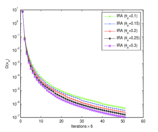
Figure 1: Example 1 with $\lambda_{n}=\frac{1}{n+1}$.

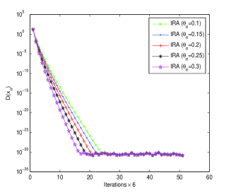
Figure 2: Example 1 with $\lambda_{n}=\frac{1}{\sqrt[10]{n+1}}$.

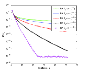
Figure 3: Example 1 with $\theta_{n}=0.1$.

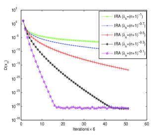
Figure 4: Example 1 with $\theta_{n}=0.3$.

Example 2. Now, consider the equilibrium problem in the Hilbert space $H=L^{2}[0,1]$ with the inner product $\left\langle x,y\right\rangle=\int_{0}^{1}x(s)y(s)ds$ and the induced norm $||x||^{2}=\int_{0}^{1}x^{2}(s)ds$. The feasible set $C$ is the unit ball $\mbox{B}[0,1]$ and the bifunction $f$ is of the form $f(x,y)=\left\langle Ax,y-x\right\rangle$ with the operator $A:H\to H$ defined by

$$A(x)(t)=\int_{0}^{1}\left[x(t)-F(t,s)f(x(s))\right]ds+g(t),~{}x\in H,~{}t\in[0,1],$$ (30)

where

$$F(t,s)=\frac{2tse^{t+s}}{e\sqrt{e^{2}-1}},~{}f(x)=\cos x,~{}g(t)=\frac{2te^{t}}{e\sqrt{e^{2}-1}}.$$

Note that $g(t)$ is chosen such that $x^{*}(t)=0$ is the solution of the problem. Since the mapping $S(x)(t)=\int_{0}^{1}F(t,s)f(x(s))ds$ is Fr$\rm\acute{e}$chet differentiable and $||S^{\prime}(x)h||\leq||x||||h||$ for all $x,~{}h\in H$. Thus, a straightforward computation implies that $f$ is monotone (so, pseudomonotone) and satisfies the Lipschitz-type condition. We do not know whether $f$ is strongly pseudomonotone or not?!, but we still wish to make numerical experiments for this example, and a fact that if yes, we also do not need to know the Lipschitz-type and strongly pseudomonotone constants of $f$. All the optimization problems in the algorithms are reduced to the projections on $C$ which are explicitly computed. The integral in (30) and others are computed by the trapezoidal formula with the stepsize $\tau=0.001$. The starting points are $x_{0}(t)=x_{1}(t)=t+0.5\cos t$. The numerical results are described in Figures 6 - 8.

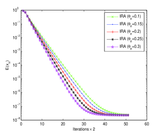
Figure 5: Example 2 with $\lambda_{n}=\frac{1}{n+1}$.

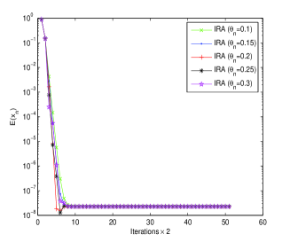
Figure 6: Example 2 with $\lambda_{n}=\frac{1}{\sqrt[10]{n+1}}$.

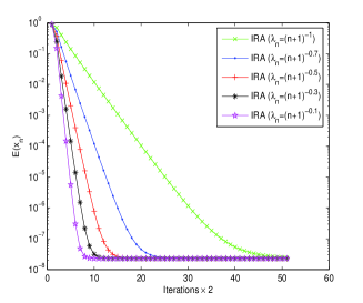
Figure 7: Example 2 with $\theta_{n}=0.1$.

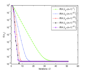
Figure 8: Example 2 with $\theta_{n}=0.3$.

From the aforementioned results, we see that the convergence rate of algorithm IRA depends strictly on the convergence rate of the sequence of stepsize $\lambda_{n}$, and that algorithm IRA seems to work better when $\lambda_{n}$ is more slowly diminishing, and also when inertial parameter $\theta_{n}$ is larger. For example, in view of Figures 2 and 2, after the first $300$ iterations, the sequence $D(x_{n})$ generated by algorithm IRA with $\lambda_{n}=\frac{1}{n+1}$ approximates $10^{-7}$ while that one with $\lambda_{n}=(n+1)^{-0.1}=\frac{1}{\sqrt[10]{n+1}}$ is $10^{-30}$.

6.2 Compare Algorithm 3.1 with others

In this part, we present several experiments in comparisons algorithm IRA with others. As mentioned above, we will compare algorithm IRA with three algorithms having the same features as RA, EGM and M-EGM. In comparisons, we use $\theta_{n}=0.3$ for algorithm IRA, and $\lambda_{n}=\frac{1}{n+1}$ or $\lambda_{n}=\frac{1}{\sqrt[10]{n+1}}$ for all the algorithms. The starting points are the same as in the previous part.
Table 1 reports the numerial results for Example 1. In this example, since the solution of problem is unknown, we have used the stopping criterion as $D(x_{n})\leq\mbox{\rm TOL}$. As in H2017AA ; H2017NUMA and the previous experiments, it is seen that the convergence rate of the algorithms depends strictly on the convergence rate of sequence of stepsize $\lambda_{n}$. So, we choose here the different tolerance TOL which is based the choice of $\lambda_{n}$. The comparisons include the number of iterations (Iter.) and the execution time in second (CPU(s)).

Table 1: A comparison between algorithm IRA (with $\theta_{n}=0.3$) and others in Example 1

			IRA (Alg. 3.1)		RA		EGM		M-EGM
$\lambda_{n}$	m	TOL	CPU(s)	Iter.	CPU(s)	Iter.	CPU(s)	Iter.	CPU(s)	Iter.
	50	$10^{-4}$	0.76	29	1.17	47	2.26	48	2.34	47
		$10^{-6}$	3.47	109	7.48	214	14.35	221	15.16	218
$\frac{1}{n+1}$	70	$10^{-4}$	1.45	34	2.02	54	4.25	56	4.41	55
		$10^{-6}$	7.02	131	14.25	256	27.30	263	28.32	260
	100	$10^{-4}$	3.54	37	5.59	64	9.88	67	9.83	66
		$10^{-6}$	16.66	148	31.07	293	62.75	299	66.16	297
	50	$10^{-20}$	2.69	55	4.57	95	9.60	104	10.09	104
		$10^{-25}$	3.41	72	6.11	123	11.51	134	11.59	134
$\frac{1}{\sqrt[10]{n+1}}$	70	$10^{-20}$	4.10	53	7.34	92	16.67	102	17.64	102
		$10^{-25}$	5.70	68	10.81	118	26.41	131	25.35	131
	100	$10^{-20}$	8.76	57	14.16	97	30.62	107	30.52	106
		$10^{-25}$	11.23	74	18.95	126	40.76	137	40.23	137

Table 2 shows the results for Example 2. The stopping criterion is used here as $E(x_{n})\leq\mbox{\rm TOL}$. In view of Tables 1 and 2, we see that algorithm IRA works the best in both number of iterations and execution time. Also, it is worth mentioning that algorithm IRA with inertial effects is better than the regularized algorithm RA which works without inertial term.

Table 2: A comparison between algorithm IRA (with $\theta_{n}=0.3$) and others in Example 2

		IRA (Alg. 3.1)		RA		EGM		M-EGM
$\lambda_{n}$	TOL	CPU(s)	Iter.	CPU(s)	Iter.	CPU(s)	Iter.	CPU(s)	Iter.
$\frac{1}{n+1}$	$10^{-5}$	4.21	38	6.44	56	13.43	63	9.03	63
	$10^{-7}$	7.41	55	10.04	83	22.74	92	14.10	92
$\frac{1}{\sqrt[10]{n+1}}$	$10^{-5}$	0.68	8	0.87	10	3.72	23	1.98	16
	$10^{-7}$	0.88	10	1.35	14	5.74	33	2.94	24

Remark 6.8

The rate of convergence proved in Theorem 5.1 shows that the smaller is the inertial parameter $\theta$, the smaller is the parameter $\alpha$ of the rate. Then, the convergence rate is better when the inertial parameter is not used, i.e., when $\theta=0$. This contradicts the numerical experiments presented in this section where the algorithm is considered with the sequence $\left\{\lambda_{n}\right\}$. This can be due to our bad choice of the rate parameter $\alpha$ (depends on $\theta$) which originates from the analyzied techniques in the paper. This also suggests for a forthcoming work to study and reanalyze Algorithm 3.1 where we can choose a function $\alpha=\alpha(\theta)$ which optimizes the convergence rate of the algorithm.

7 Conclusions

The paper has proposed a new inertial regularized algorithm for solving strongly pseudomonotone and Lipschitz-type equilibrium problems. The algorithm is a combination between the proximal-like regularized technique and inertial effects. By using a sequence of stepsizes being diminishing and non-summable, the proposed algorithm can be done without the prior knowledge of the modulus of strong pseudomonotonicity and the Lipschitz-type constant of cost bifunction. Theorem of strong convergence has been proved. In the case, when those constants are known, we have established the rate of linear convergence of the algorithm. Several numerical results have been reported to illustrate the computational performance of the algorithm in comparisons with other algorithms. These numerical results have also confirmed that the algorithm with inertial effects seems to work better than without inertial effects.

Disclosure statement

No potential conflict of interest was reported by the author.

References

• (1) Alvarez, F., Attouch, H.: An inertial proximal method for maximal monotone operators via discretization of a nonlinear oscillator with damping. Set-Valued Anal. 9, 3-11 (2001)
• (2) Alvarez, F.: Weak convergence of a relaxed and inertial hybrid projection-proximal point algorithm for maximal monotone operators in Hilbert space. SIAM J. Optim. 14, 773-782 (2004)
• (3) Anh, P.N.: A hybrid extragradient method extended to fixed point problems and equilibrium problems. Optimization 62, 271-283 (2013)
• (4) Antipin, A.S.: On convergence of proximal methods to fixed points of extremal mappings and estimates of their rate of convergence. Comp. Maths. Math. Phys. 35, 539-551 (1995)
• (5) Bauschke, H.H., Combettes, P.L.: Convex Analysis and Monotone Operator Theory in Hilbert Spaces. Springer, New York (2011)
• (6) Blum, E., Oettli, W.: From optimization and variational inequalities to equilibrium problems. Math. Program. 63, 123-145 (1994)
• (7) Bigi, G., Castellani, M., Pappalardo, M., Passacantando, M.: Existence and solution methods for equilibria, European J. Oper. Res. 227, 1-11 (2013)
• (8) Bigi, G., Castellani, M., Pappalardo, M.: A new solution method for equilibrium problems. Optim. Meth. Software 24, 895-911 (2009)
• (9) Bigi G., Passacantando M.: Descent and penalization techniques for equilibrium problems with nonlinear constraints. J. Optim. Theory Appl. 164, 804-818 (2015)
• (10) Bigi G., Passacantando M.: Gap functions and penalization for solving equilibrium problems with nonlinear constraints. Comput. Optim. Appl. 53, 323-346 (2012)
• (11) Bot, R.I., Csetnek, E.R., Laszlo, S.C.: An inertial forward-backward algorithm for the minimization of the sum of two nonconvex functions. EURO J. Comput. Optim. 4, 3-25 (2016)
• (12) Charitha, C.: A note on D-gap functions for equilibrium problems. Optimization 62, 211-226 (2013)
• (13) Combettes, P. L., Hirstoaga, S. A.: Equilibrium programming in Hilbert spaces. J. Nonlinear Convex Anal. 6(1), 117-136 (2005)
• (14) Contreras, J., Klusch, M., Krawczyk, J.B.: Numerical solutions to Nash-Cournot equilibria in coupled constraint electricity markets. IEEE Trans. Power Syst. 19 (1), 195-206 (2004)
• (15) Di Lorenzo D., Passacantando M., Sciandrone M.: A convergent inexact solution method for equilibrium problems. Optim. Meth. Software 29, 979-991 (2014)
• (16) Facchinei F, Pang JS. Finite-Dimensional Variational Inequalities and Complementarity Problems, Springer, Berlin (2002)
• (17) Fan, K.: A minimax inequality and applications, In: Shisha, O. (ed.) Inequality, III, Academic Press, New York, 103-113 (1972)
• (18) Flam, S.D., Antipin, A.S.: Equilibrium programming and proximal-like algorithms. Math. Program. 78, 29-41 (1997)
• (19) Hieu, D. V.: New extragradient method for a class of equilibrium problems in Hilbert spaces. Appl. Anal. 97, 811-824 (2018)
• (20) Hieu, D. V.: Convergence analysis of a new algorithm for strongly pseudomontone equilibrium problems. Numer. Algor. 77, 983-1001 (2018)
• (21) Hieu, D.V., Muu, L. D, Anh, P. K.: Parallel hybrid extragradient methods for pseudomonotone equilibrium problems and nonexpansive mappings. Numer. Algorithms 73, 197-217 (2016)
• (22) Hieu, D.V.: New subgradient extragradient methods for common solutions to equilibrium problems. Comput. Optim. Appl. 67, 571-594 (2017)
• (23) Hieu, D.V.: An extension of hybrid method without extrapolation step to equilibrium problems. J. Ind. Manag. Optim. 13, 1723-1741 (2017)
• (24) Hieu, D.V.: Halpern subgradient extragradient method extended to equilibrium problems. Rev. R. Acad. Cienc. Exactas Fís. Nat. Ser. A Math. RACSAM. 111, 823-840 (2017)
• (25) Hieu, D.V.: Hybrid projection methods for equilibrium problems with non-Lipschitz type bifunctions. Math. Meth. Appl. Sci. 40, 4065-4079 (2017)
• (26) Hieu, D.V.: Parallel extragradient-proximal methods for split equilibrium problems. Math. Model. Anal. 21, 478-501 (2016)
• (27) Konnov I. V.: Application of the proximal point method to non-monotone equilibrium problems. J. Optim. Theory Appl. 119, 317-333 (2003)
• (28) Konnov, I.V.: Equilibrium Models and Variational Inequalities. Elsevier, Amsterdam (2007)
• (29) Konnov, I. V., Ali, M. S. S.: Descent methods for monotone equilibrium problems in Banach spaces. J. Comput. Appl. Math. 188, 165-179 (2006)
• (30) Konnov, I. V., Pinyagina, O.V.: D-gap functions and descent methods for a class of monotone equilibrium problems. Lobachevskii J. Math. 13, 57-65 (2003)
• (31) Korpelevich, G. M.: The extragradient method for finding saddle points and other problems, Ekonomikai Matematicheskie Metody. 12, 747-756 (1976)
• (32) Lyashko, S. I, Semenov, V. V.: Optimization and Its Applications in Control and Data Sciences. Springer, Switzerland, Volume 115, 315-325 (2016)
• (33) Maingé P-E, Moudafi A.: Convergence of new inertial proximal methods for dc programming. SIAM J Optim 19, 397-413 (2008)
• (34) Mastroeni, G.: On auxiliary principle for equilibrium problems. In: P. Daniele, F. Giannessi, A. Maugeri (editors), Equilibrium problems and variational models, Kluwer Academic, 289-298 (2003)
• (35) Mastroeni, G.: Gap function for equilibrium problems. J. Global. Optim. 27, 411-426 (2003)
• (36) Martinet, B.: R$\rm\acute{e}$gularisation d$\rm\acute{}$ in$\rm\acute{e}$quations variationelles par approximations successives. Rev. Fr. Autom. Inform. Rech. Op$\rm\acute{e}$r., Anal. Num$\rm\acute{e}$r. 4, 154-159 (1970)
• (37) Moudafi, A.: Proximal point algorithm extended to equilibrum problem. J. Nat. Geometry, 15, 91-100 (1999)
• (38) Moudafi, A.: Second-order differential proximal methods for equilibrium problems. J. Inequal. Pure and Appl. Math. 4, Art. 18 (2003)
• (39) Muu, L.D., Oettli, W.: Convergence of an adative penalty scheme for finding constrained equilibria. Nonlinear Anal. TMA 18 (12), 1159-1166 (1992)
• (40) Muu, L.D., Quoc, T.D.: Regularization algorithms for solving monotone Ky Fan inequalities with application to a Nash-Cournot equilibrium model. J. Optim. Theory Appl. 142, 185-204 (2009)
• (41) Nikaido, H., Isoda, K.: Note on noncooperative convex games, Pacific J. Math. 5, 807-815 (1955)
• (42) Quoc, T.D., Muu, L.D., Nguyen, V.H.: Extragradient algorithms extended to equilibrium problems. Optimization 57, 749-776 (2008)
• (43) Rockafellar, R.T.: Monotone operators and the proximal point algorithm. SIAM J. Control Optim. 14, 877–898 (1976)
• (44) Santos, P., Scheimberg, S.: An inexact subgradient algorithm for equilibrium problems. Comput. Appl. Math. 30, 91-107 (2011)
• (45) Strodiot, J.J., Nguyen, T.T.V., Nguyen, V.H.: A new class of hybrid extragradient algorithms for solving quasi-equilibrium problems. J. Glob. Optim. 56, 373-397 (2013)
• (46) Strodiot, J.J., Vuong, P.T., Nguyen, T.T.V.: A class of shrinking projection extragradient methods for solving non-monotone equilibrium pro blems in Hilbert spaces. J. Glob. Optim. 64, 159-178 (2016)