M0.20$-$0.033: An Expanding Molecular Shell in the Galactic Center Radio Arc

Abstract

We present high-frequency Karl G. Jansky Very Large Array (VLA) continuum and spectral line (NH₃, H64$\alpha$, and H63$\alpha$) observations of the Galactic Center Radio Arc region, covering the Sickle H II region, the Quintuplet cluster, and molecular clouds M0.20$-$0.033 and M0.10$-$0.08. These observations show that the two velocity components of M0.20$-$0.033 ($\sim$25 & 80 km s^-1), previously thought to be separate clouds along the same line-of-sight, are physically connected in position-velocity space via a third southern component around 50 km s^-1. Further position-velocity analysis of the surrounding region, using lower-resolution survey observations taken with the Mopra and ATCA telescopes, indicates that both molecular components in M0.20$-$0.033 are physically connected to the M0.10$-$0.08 molecular cloud, which is suggested to be located on stream 1 in the Kruijssen et al. (2015) orbital model. The morphology and kinematics of the molecular gas in M0.20$-$0.033 indicate that the two velocity components in M0.20$-$0.033 constitute an expanding shell. Our observations suggest that the M0.20$-$0.033 expanding shell has an expansion velocity of 40 km s^-1, with a systemic velocity of 53 km s^-1, comparable to velocities detected in M0.10$-$0.08. The origin of the expanding shell is located near the Quintuplet cluster, suggesting that the energy and momentum output from this massive stellar cluster may have contributed to the expansion.

1 Introduction

The central molecular zone of the Galactic center (GC; a region $\sim$200 pc in extent) is known to be an extreme Galactic environment. Molecular clouds (MCs) in the GC are believed to have hotter gas temperatures (50$-$300 K; Mauersberger et al., 1986; Mills & Morris, 2013; Krieger et al., 2017), higher densities ($10^{4-5}$ cm^-3; Zylka et al., 1992), and broader line widths ($\sim$20$-$50 km s^-1; Bally et al., 1987) than clouds in the disk ($\sim$10$-$20 K, $10^{2-3}$ cm^-3, $\sim$1$-$10 km s^-1; Hüttemeister et al., 1993; Oka et al., 2001b; Longmore et al., 2013). The connection between these individual clouds and the larger structure of molecular gas in the GC is an area of active study (Molinari et al., 2011; Kruijssen et al., 2015). The molecular gas has been modeled as several ‘orbital streams’ by using the central velocities of the individual gas clouds and projecting their distances from Sgr A^∗. In some cases, the complex kinematics of the molecular gas in the GC, caused by local sources of energy injection, makes modeling the overall distribution of the molecular gas challenging.

The GC Radio Arc is located $\sim$25 pc in projection from Sgr A^∗  and is one of the regions where modeling the orbital stream is difficult. The Radio Arc region includes an extended MC (M0.20$-$0.033; Serabyn & Guesten, 1991; Serabyn & Morris, 1994), the Sickle H II region (G0.18$-$0.04; Yusef-Zadeh & Morris, 1987; Lang et al., 1997), and the Quintuplet cluster (Figer et al., 1999a). The Lyman continuum ionizing rate of the Sickle H II region (2.8$\times$10⁴⁹ photons s^-1) indicates the H II region is the result of ionization from the adjacent Quintuplet cluster heating the edge of M0.20$-$0.033 (Serabyn & Guesten, 1991; Lang et al., 1997). The southern extent of the Radio Arc region includes the core of a dense MC (M0.10$-$0.08). Single-dish ($\sim$35$-$18″ resolution) observations of H¹³CO⁺ (J=1$-0$) and SiO (J=1$-0$) show that M0.10$-$0.08 is a denser clump of a larger diffuse cloud (Tsuboi et al., 1997; Handa et al., 2006; Tsuboi et al., 2011).

Figure 1 (top) illustrates the orbital model proposed by Kruijssen et al. (2015) (their Figure 6). Figure 1 (bottom) shows the molecular gas velocities (data points) compared to the Kruijssen et al. (2015) orbital model (solid lines) from their Figure 4. At the location of the Radio Arc region there are two velocity components in the molecular gas, at $\sim$25 & 80 km s^-1 (M0.20$-$0.033, red box in Figure 1, bottom). Kruijssen et al. (2015) attributes these two components to being on the near side (80 km s^-1; stream 1) and far side (25 km s^-1; stream 3) of the GC (red box in Figure 1, top).

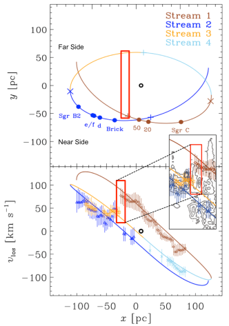
Figure 1: Orbital model from Figures 6 & 4 in Kruijssen et al. (2015), showing the spatial orientation (top) and velocity distribution (bottom), respectively. In their model the GC molecular gas has an open orbit solution that is divided into four orbital streams. The data points in the bottom panel show the observed molecular gas velocities compared to the modeled orbital streams (solid line). The red box in both panels shows the velocities (bottom) and locations (top) of the two molecular components in M0.20$-$0.033. (inset): [CII] contours from Langer et al. (2017) (cropped from their Figure 7), overlaid on the Kruijssen et al. (2015) orbital model.

We use high-resolution Karl G. Jansky Very Large Array (hereafter, VLA) observations, a facility operated by the National Radio Astronomy Observatory (NRAO), to investigate the complex kinematics in the Radio Arc region and how massive star clusters influence the GC ISM. In this paper we present the 24.5 GHz continuum and spectral line results for the Radio Arc region (Sections 3 & 4, respectively). All results presented in this paper are discussed in Section 5.

2 Observations and Data Calibration

2.1 Observational Set up

We used the WIDAR correlator of the VLA to simultaneously obtain wide bandwidth continuum and multiple spectral lines in the Radio Arc region. The data were taken with the K band receiver (18.0$-$26.5 GHz) on 2012 January 14. All observations used the hybrid DnC array in order to compensate for the low altitude of the GC at the VLA site. The radio observation subbands presented in this paper were centered at 24.054 and 25.374 GHz, each with a bandwidth of 0.84 GHz that is segmented into seven spectral windows. Two additional spectral windows were observed at X band ($\sim$8 GHz) to determine the pointing accuracy during the observations. We had 512 channels per spectral window in each subband, with a corresponding spectral resolution of 250 kHz ($\sim$3 km s^-1). This spectral configuration enabled us to accurately observe the NH₃ (3,3), H64$\alpha$, and H63$\alpha$ spectral lines. The NH₃ (3,3) transition (hereafter, NH₃), has a rest frequency of 23.87013 GHz. The H64$\alpha$ and H63$\alpha$ radio recombination lines have a rest frequency of 24.50990 GHz and 25.68628 GHz, respectively. The primary beam FWHM is $\sim$$3\farcm 4$ at K band, therefore six Nyquist sampled pointings were needed to survey the region with a total of $\sim$25 minutes on source per pointing.

2.2 Calibration and Imaging

We used the Common Astronomy Software Application (CASA) program provided by NRAO to perform all rudimentary calibration steps (i.e., bandpass, flux, and phase corrections), as well as correcting for atmospheric opacity and antenna delay solutions. These additional corrections were needed due to the increased water vapor opacity at higher VLA frequencies. These observations used 3C286 as the absolute flux calibrator and J1733-1304 as the bandpass calibrator. Our phase calibrator, J1744-3166, was observed at 25 minute intervals.

All continuum and molecular transitions were imaged using the CASA task CLEAN. Since all of the regions surveyed required multiple pointings, the CLEAN parameter ‘mosaic’ was used to combine the observed fields. The continuum images were obtained by flagging out all spectral lines and end channels. We used ‘briggs’ weighting with a ‘robust’ parameter of 0.5 to balance our point-source resolution ($1\farcs 86$$\times$$2\farcs 18$) with the sensitivity of the image (50 $\mu$Jy beam^-1, rms noise).

The spectral lines were first continuum subtracted using the CASA task IMCONTSUB on line-free channels. Spectral lines were imaged using their natural frequency resolution with no spectral smoothing and ‘natural’ weighting for all transitions. The spectral images for NH₃, H64$\alpha$, and H63$\alpha$ were then spatially smoothed from their natural resolution to boost the low signal-to-noise ratios (SNRs) in the Radio Arc region, resulting in a spatial resolution of 5$\farcs$0$-$5$\farcs$7. Due to the extended nature of the NH₃ emission, we used the CLEAN parameter ‘multiscale’ to maximize the sensitivity to large-scale diffuse structures in the images (where the largest angular size is $\sim$60″). The H64$\alpha$ and H63$\alpha$ recombination lines were averaged in the image plane to boost our SNR, using the CASA task IMMATH.

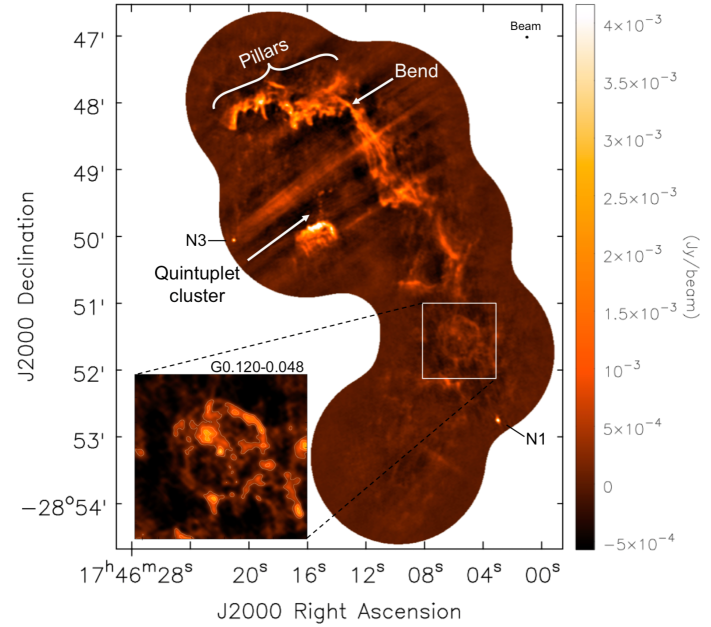
Figure 2: 24.5 GHz continuum image of the Sickle H II region and M0.10$-$0.08 (southernmost field), using 2 GHz bandwidth. Labeled are several features discussed in Section 3. (inset): The luminous blue variable: G0.120$-$0.048, at higher contrast, with grey contours showing: 4, 7, & 10 $\times$ 50 $\mu$Jy beam^-1 (rms noise). The restoring beam, shown in the top right corner, is $2\farcs 18$$\times$$1\farcs 86$, PA=82$\fdg$8.

3 Radio Continuum Emission

Figure 2 shows the 24.5 GHz continuum emission in the Radio Arc and M0.10$-$0.08 regions. The large-scale curved structure ($\sim$5′; 12 pc) in the four northern fields is the Sickle H II region (G0.18$-$0.04; Yusef-Zadeh & Morris, 1987; Lang et al., 1997). The Sickle H II region has several distinct features (indicated in Figure 2): the ‘Sickle H II pillars,’ the ‘Bend,’ and the striations associated with the non-thermal filaments (NTFs). The radio continuum emission in the Sickle H II region is clumpy in nature, with several knots of emission that are oriented along the southern edge of the pillars region. Several of these clumps protrude from the Sickle H II region towards decreasing declination, resulting in the pillar-like appearance. These pillar-like features are $\sim$10$-$20″ (0.4$-$0.8 pc) in length, with a width of $\sim$2$-$10″ (0.08$-$0.4 pc). Many of these pillars show a continuum brightening near one end. The $\sim$$90\arcdeg$ Bend in the Sickle H II region appears to separate the clumpy material in the Sickle H II pillars from the southern striations.

We also detect several Radio Arc NTFs at 24.5 GHz (Yusef-Zadeh & Morris, 1987). These NTFs are oriented perpendicular to the western portion of the the Sickle H II region and Galactic plane, as seen in Figure 2. At the apparent intersection of the NTFs and the Sickle H II region, there are several bright, compact knots of emission. Located along one of these NTFs is the Pistol nebula (Figer et al., 1999b), which contains the brightest diffuse emission in the entire Radio Arc region. North of the Pistol nebula are several point-like radio sources, produced by the stellar winds of massive stars from the Quintuplet cluster (Lang et al., 2005).

Located near the edge of our primary beam are two bright point sources: N1 and N3. These two unresolved sources contain the brightest compact emission in the Radio Arc region. When comparing the radio emission to Paschen-$\alpha$ (hereafter, P$\alpha$) emission in Wang et al. (2010), N1 has a P$\alpha$ counterpart, indicating that it is thermal in nature. N3 does not have a P$\alpha$ counterpart, suggesting that it is non-thermal in nature. This is consistent with the high frequency (10$-$49 GHz) spectral index of N3 ($\alpha=-$0.8; Ludovici et al., 2016).

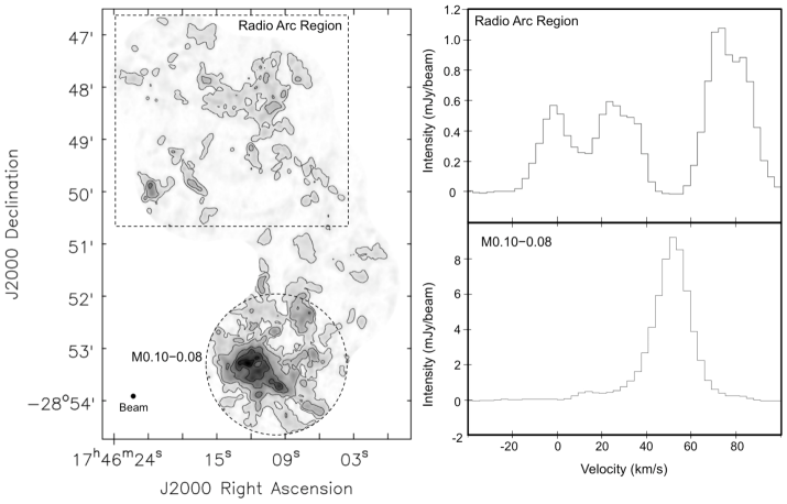
Figure 3: (left): maximum intensity NH₃ (3,3) emission ($5\farcs 0\times 5\farcs 0$, PA=0$\fdg$0, resolution), integrated over a velocity range of -20$-$100 km s^-1, with contours showing: 5, 15, 50, 100, & 200 $\times$ 3 mJy beam^-1 (rms noise). (right): spectra integrated over the outlined regions shown on the left for the Radio Arc region (top) and M0.10$-$0.08 (bottom).

The M0.10$-$0.08 MC is located in the southernmost field in Figure 2 and has very low-level continuum compared to the rest of the emission in the image. There is a very faint filamentary streak near the right edge of this field. At 0.3 mJy beam^-1, this feature is the only emission in this field that is detected above 5$\sigma$. This continuum feature is also seen in the P$\alpha$ emission from Wang et al. (2010), indicating that it is thermal in nature.

We also present the first radio detection of the recently discovered, isolated, luminous blue variable: G0.120$-$0.048 (Mauerhan et al., 2010; Lau et al., 2014) and surrounding shell (Figure 2, inset). Unlike the ejected material from the Pistol star (the Pistol nebula; G0.15$-$0.05), the shell surrounding G0.120$-$0.048 has a circular structure that is also seen in P$\alpha$ (Mauerhan et al., 2010). This circular structure suggests that the shell has not strongly interacted with the asymmetrically distributed ISM material that would distort the symmetric shape. The G0.120$-$0.048 shell is 37″ (1.4 pc) in diameter and shows a slight continuum brightening on the northern edge.

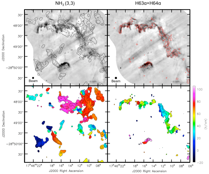
Figure 4: Distribution of NH₃ (3,3) ($5\farcs 0$$\times$$5\farcs 0$, PA=0$\fdg$0, resolution, left panels) and combined H63$\alpha$+H64$\alpha$ radio recombination lines ($5\farcs 68$$\times$$5\farcs 61$, PA=88$\fdg$5, resolution, right panels). The top panels show maximum intensity contours in: NH₃ at 5, 10, 20, & 50 $\times$ 3 mJy beam^-1 (rms level), and the combined H63$\alpha$+H64$\alpha$ radio recombination lines at 5, 6, 8, & 10 $\times$ 1.1 mJy beam^-1 (rms level) overlaid on the 24.5 GHz radio continuum, shown in greyscale. The bottom panels show the same maximum intensity contours, now overlaid on the intensity-weighted velocity distribution for emission between -20$-$100 km s^-1.

4 Spectral Line Emission

Figure 3 (left) shows widespread NH₃ emission throughout our surveyed regions, where the brightest emission is associated with M0.10$-$0.08. The NH₃ emission in M0.10$-$0.08 is over five times brighter than emission detected in the Radio Arc region. Figure 3 (right) shows spectral profiles integrated over the two regions indicated in the emission map. The NH₃ spectrum of the Radio Arc region shows three velocity components: -15$-$15 km s^-1, 15$-$40 km s^-1, and 60$-$90 km s^-1 (Figure 3, top right). The 15$-$40 km s^-1 and 60$-$90 km s^-1 molecular components are known to be associated with M0.20$-$0.033 (Serabyn & Guesten, 1991). Hereafter, the molecular gas features associated with the 15$-$40 km s^-1 and 60$-$90 km s^-1 emission will be identified as the ‘low-velocity’ and ‘high-velocity’ molecular components, respectively. The M0.10$-$0.08 spectrum (Figure 3, bottom right) shows most of the NH₃ emission is contained within a single component that ranges in velocity from $\sim$35$-$70 km s^-1, that peaks in intensity around 55 km s^-1. This velocity has an intermediate value between the low- and high-velocity molecular components in M0.20$-$0.033.

Figure 4 presents the NH₃ (left) and the combined H64$\alpha$ and H63$\alpha$ radio recombination lines (right) in the Radio Arc region. The top panels in Figure 4 show the distribution of the spectral line emission with respect to the 24.5 GHz continuum features. The bottom panels in Figure 4 show the velocity distribution of the spectral line emission.

4.1 Morphology and Kinematics of Molecular Gas

Most of the NH₃ emission in the Radio Arc region is associated with M0.20$-$0.033, as shown by the velocity distribution in Figure 4 (bottom left). The velocity distribution shows that most of the compact NH₃ emission in M0.20$-$0.033 is associated with the high-velocity molecular component, consistent with the integrated spectrum (Figure 3, top right). The largest emission region in the high velocity molecular component is $\sim$2$\arcmin$ (4.7 pc) in length and spatially overlaps with the western side of the Sickle H II pillars (Figure 4, top left). Very little NH₃ emission is detected near the eastern side of the Sickle H II pillars. The emission associated with the low-velocity molecular component of M0.20$-$0.033 (Figure 4, bottom left) is distributed in low level ($<$10$\sigma$) disjointed clumps that are $\sim$30″ or less in extent. The NH₃ emission associated with the -$15$$-$15 km s^-1 molecular component is primarily located in the N3 MC (M0.17$-$0.08; Ludovici et al., 2016). The NH₃ emission in the N3 MC is the brightest emission detected in Figure 4. There are also a few, faint, isolated clumps of emission at this velocity range that are located between the N3 MC and the Sickle H II pillars.

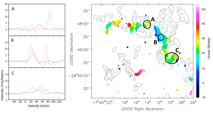
Figure 5: (left): spectra of both the molecular (red: NH₃ (3,3)) and ionized (blue: H63$\alpha$+H64$\alpha$) gas toward the Sickle H II region. (right): color scale shows the intensity-weighted velocity distribution of the combined H63$\alpha$+H64$\alpha$ radio recombination lines over -20$-$100 km s^-1, with black contours of the NH₃ (3,3) emission at 5, 10, 20, & 50 $\times$ 3 mJy beam^-1. The contours and color scale in right are from Figure 4, top left and bottom right, respectively.

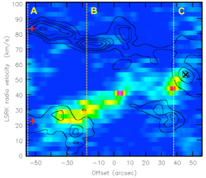
Figure 6: Position-velocity comparison of the ionized gas (color scale: H63$\alpha$+H64$\alpha$; width=18″) and the molecular gas (black contours: NH₃; width=41″) from 17^h46^m12$\fs$9, -28°48′02$\farcs$7 ($-$50 offset) to 17^h46^m09$\fs$1 -28°49′25$\farcs$8 (+50 offset). The spectral and spatial resolution for both transitions are $\sim$3 km s^-1 and $\sim$5″, respectively (see Section 2). The three yellow vertical dashed lines show the relative locations of the three regions in Figure 5. The red “$+$” signs mark the midpoint of the ellipse discussed in Section 5.2.2. The black “$\times$” sign indicates the edge of ellipse, also discussed in Section 5.2.2.

4.2 Morphology and Kinematics of Ionized Gas

Figure 4 (right) shows the ionized gas emission, as traced by the combined H64$\alpha$ and H63$\alpha$ radio recombination lines. Figure 4 (top right) shows that the morphology of the ionized gas emission follows the continuum emission. The brightest ionized gas emission in the Radio Arc region ($>$11 mJy beam^-1) coincides with the Pistol nebula. Ionized gas intensities in the Sickle H II region range from 6$-$10 mJy beam^-1. Central velocities fit to the ionized gas profiles in the Sickle H II region and Pistol nebula range from 15$-$75 km s^-1 and 80$-$150 km s^-1, respectively (Figure 4, bottom right). The velocity of the ionized gas in the Sickle H II pillars are typically higher (30$-$80 km s^-1) than velocities in the southern regions of the Sickle H II region (15$-$55 km s^-1). These velocities in the southern region of the Sickle H II region are increasing from $\sim$15 km s^-1 (at the Bend) to $\sim$55 km s^-1 in the direction of Sgr A^∗, for a gradient of $\sim$10 km s^-1 pc^-1 parallel to the Galactic plane. The ionized gas velocities in the Sickle H II pillars do not appear to follow a gradient, as seen in the southern regions, but are disjointed in velocity space at our resolution. We do not detect any emission above 5.5 mJy beam^-1 (5$\sigma$) from G0.120$-$0.048 or the surrounding shell. We also do not detect any ionized gas emission above 5$\sigma$ associated with the point source N3 or the M0.10$-$0.08 MC.

4.3 Comparison of Ionized and Molecular Gas along the Sickle H II region

Figure 5 (right) shows the spatial distribution of the molecular and ionized gas emission. The three selected locations, labeled A$-$C, were chosen because they contain both M0.20$-$0.033 molecular components and an ionized gas component. The molecular and ionized spectra for each location are shown as panels in Figure 5 (left). At all three locations we detect only one ionized component and 2$-$3 molecular components.

At region A, the high-velocity molecular component is roughly three times brighter than the low-velocity molecular component. The ionized gas emission is located at intermediate-velocities between the two components and is not associated with a single molecular component. Region B shows a comparable intensity between the low- and high-velocity molecular components. However, the velocity profile of the low-velocity molecular component is broader ($\sim$20 km s^-1) than the high-velocity molecular component ($\sim$10 km s^-1). The low-velocity molecular component also correlates fairly closely with the ionized gas emission (Figure 5).

The southernmost region, C, has the most complex molecular kinematics out these three regions. At region C there is a third molecular component (45$-$65 km s^-1) that is not detected in regions A & B. This ‘intermediate-velocity’ molecular component peaks in intensity around 55 km s^-1, similar to the molecular emission detected in M0.10$-$0.08 (Figure 3, bottom right). Region C is also located the closest in projection to M0.10$-$0.08 out of all three regions. The ionized gas in region C, overlaps in velocity space with the low- and intermediate-velocity molecular components. However, since the ionized gas emission peaks between these two components (at $\sim$45 km s^-1), it is not solely associated with either molecular component (compared to the ionized gas at region B).

Figure 6 compares the position and velocity distribution of the molecular and ionized emission along the Sickle H II region (from regions A$-$C). The high-velocity molecular component shows continuous emission along this region that is increasing in velocity from region C ($\sim$55 km s^-1) to region A ($\sim$90 km s^-1). The ionized gas also shows continuous emission along the same path, but is decreasing in velocity from region C ($\sim$60 km s^-1) to region A ($\sim$15 km s^-1), consistent with the gradient described in Section 4.2. The low-velocity molecular component is detected in small, disjointed clumps that are closely correlated in both position and velocity with the ionized gas emission. Both of these described velocity gradients, shown in Figure 6, are comparable in magnitude ($\sim$10 km s^-1 pc^-1) but opposite in sign. Further, these two velocity gradients are shown to spatially overlap in both position and velocity near region C.

5 Discussion

5.1 Arrangement of Gas Components in M0.20$-$0.033

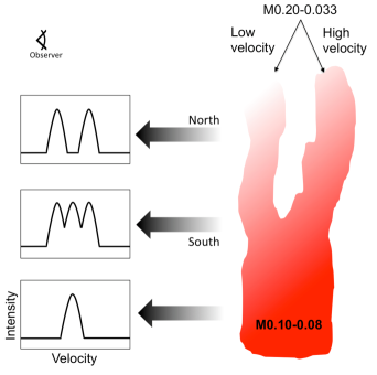
Figure 7: Schematic of the proposed possible arrangement of molecular components in M0.20$-$0.033 and M0.10$-$0.08 (see Section 5.1). The panels on the left show what the spectra for integrated regions in the proposed arrangement might look like, with the arrows indicating the corresponding region of the molecular gas.

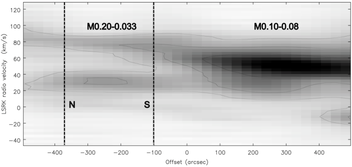
Figure 8: Position-velocity diagram of NH₃ (3,3) observed with the single-dish Mopra telescope as part of the HOPS survey ($\sim$2′ resolution; Walsh et al., 2011a). The emission covers a galactic longitude from 0$\fdg$025 (+450″ offset) to 0$\fdg$3 ($-$450″ offset), and is integrated over a 0$\fdg$15 wide slice, at a latitude of $b=-$0$\fdg$075. The vertical dashed lines represent the north (N) and south (S) regions of the cloud, as illustrated in Figure 7.

5.1.1 Physical Connection Between Low- and High-Velocity Components

Figure 6 shows two velocity gradients: a gradient increasing from C to A ($\sim$55$-$90 km s^-1; the high-velocity component) and a gradient decreasing from C to A ($\sim$60$-$15 km s^-1; the low-velocity component). These two velocity gradients spatially overlap in position-velocity space at an offset of $\sim$45″ in Figure 6 (i.e., near C). At this location we detect a faint bridge of continuous emission ranging in velocity from $\sim$35$-$80 km s^-1 over a distance of $\sim$10″. This large range of velocities is consistent with the spectrum of the molecular and ionized gas at region C in Figure 5. This spectrum shows continuous emission via a third intermediate-velocity molecular component around 55 km s^-1, which bridges the low- and high-velocity molecular components. Therefore, the bridge in position-velocity space suggests the two velocity components are physically connected near region C. The absence of this intermediate-velocity molecular component at regions A & B indicates the two velocity components are physically separated at these locations.

Figure 7 shows a schematic of the proposed possible arrangement of molecular components in M0.20$-$0.033 and M0.10$-$0.08 (see Section 5.1). The panels on the left show what the spectra for integrated regions in the proposed arrangement might look like, with the arrows indicating the corresponding region of the molecular gas based on data presented in Figure 5 and 6. For example, the profiles for Regions A and B in Figure 5 are illustrated by the ‘North’ M0.20$-$0.033 profile at the top of Figure 7. The proposed spectrum of molecular emission for Region C in Figure 5 is illustrated by the ‘South’ M0.20$-$0.033 profile in Figure 7, and the proposed spectrum for M0.10$-$0.08 is represented by the lower profile in Figure 7.

In the north of M0.20$-$0.033, our simple interpretation is that these molecular components may lie at physically different distances but are part of the same molecular structure. In contrast, our simple interpretation of the triple-peaked profile in the south of M0.20$-$0.033 is that the profile represents a superposition of the two molecular components from M0.20$-$0.033 as well as the molecular gas at an intermediate velocity, possibly associated with M0.10$-$0.08. However, the sight line to the GC is incredibly complex, and we acknowledge that our interpretation may be oversimplified. The discussion that follows is an attempt to quantify and characterize the arrangement in more detail.

However, it is important to note that we also have kinematic information of the ionized gas as well. Region A in Figure 5 shows two molecular components (as depicted in the north of Figure 7) with an intermediate-velocity ionized gas component. The combination of these three components (two molecular and one ionized) results in continuous emission, from $\sim$15 to 90 km s^-1, in the northern region of M0.20$-$0.033. This bridging of the two molecular components by an ionized gas component may be an indication that the emission in M0.20$-$0.033 is also physically connected in the north. This possible connection in the north, via an intermediate-velocity ionized gas component, is consistent with the gas distribution shown in Figure 4. For example, the bright clump of high-velocity ionized gas emission in the the Sickle H II pillars ($\sim$80 km s^-1; 17^h46^m17$\fs$5, $-$28°48′10″) is spatially adjacent to the large structure of high-velocity molecular emission evident in Figures 4 & 5, indicating that this feature is likely to be more closely related to the high-velocity molecular component than the low-velocity molecular component. A more detailed discussion of the ionized gas emission is presented in Section 5.3.2.

5.1.2 The Orbital Stream: Connection of M0.20$-$0.033 to Nearby Molecular Clouds

The molecular spectrum of M0.10$-$0.08 shows a single velocity component, $\sim$55 km s^-1, located between the low- and high-velocity components of M0.20$-$0.033 (Figure 3, right). The southern region of M0.20$-$0.033 is closest in projection to M0.10$-$0.08, suggesting the intermediate-velocity spectral feature detected toward region C might be an extension of emission from M0.10$-$0.08. Figure 7 further illustrates a possible relationship of the two velocity components of M0.20$-$0.033 to M0.10$-$0.08. In this schematic both velocity components of M0.20$-$0.033 are physically connected to M0.10$-$0.08.

The connection between M0.10$-$0.08 and the high-velocity molecular component in M0.20$-$0.033 is also posited in the Kruijssen et al. (2015) orbital model, which places both on the near side of the GC (stream 1). The low-velocity molecular component of M0.20$-$0.033, however, is proposed to be located on the far side of the GC in the Kruijssen et al. (2015) orbital model (stream 3). However, the data presented here and the single-dish observations of Serabyn & Guesten (1991) indicate that the two molecular components in M0.20$-$0.033 are spatially connected as they show continuous emission in position-velocity space (Section 5.1.1).

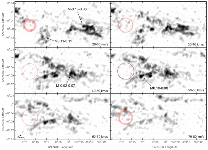
Figure 9: Maximum intensity NH₃ (3,3) emission from ATCA (SWAG survey; angular resolution of $\sim$20″ (bottom left corner); Ott et al., 2017) integrated over $\Delta$v=10 km s^-1 intervals, as indicated in the bottom right corners. The black contours show: 5, 25, & 75 $\times$ 15 mJy beam^-1 (average rms noise over all panels). The black dashed circle shows the size of the expanding shell at the systemic velocity (53 km s^-1; see Section 5.2.2). The red shaded annuli represented the predicted sizes of the shell over different velocity ranges and a spherical geometry (see Appendix A.1).

In order to further investigate the proposed connection between M0.20$-$0.033 and nearby clouds in the region, we incorporate observations made with the Mopra single-dish telescope. Figure 8 shows the position-velocity distribution of the large-scale cloud structures from M0.20$-$0.033 to M0.10$-$0.08. This position-velocity diagram covers a larger and wider spatial range than Serabyn & Guesten (1991), who focused on the region around M0.20$-$0.033 (see their Figures 2 & 4). Figure 8 supports the interpretation that the two velocity components in M0.20$-$0.033 are physically connected in the south near M0.10$-$0.08. Figure 8 also shows that the molecular gas appears to be physically connected between M0.20$-$0.033  and M0.10$-$0.08, further supporting the hypothesis that the two clouds reside along the same GC stream (stream 1 of Kruijssen et al., 2015). While these single-dish Mopra observations (Figure 8) are consistent with the kinematic structure inferred from our VLA observations (Figure 6), many of the small-scale features ($<$1′$-$2′) are not detected at the resolution of MOPRA. Therefore, we turn to a survey having intermediate resolution, and which therefore shows the relationship between large ($\sim$1′$-$2′) and small ($\sim$10″$-$20″) scale structures.

Figure 9 shows the NH₃ (3,3) distribution from the ATCA telescope, over a velocity range of $\sim$20$-$80 km s^-1. This velocity coverage includes both the low- and high-velocity molecular components of M0.20$-$0.033. The molecular emission generally appears to be concentrated towards the eastern Galactic side of the observed region at higher velocities (e.g., v $>$ 60 km s^-1). The brighter molecular emission at low velocities (e.g., v $<$ 30 km s^-1) is mainly concentrated towards the western Galactic side (e.g., M$-$0.13$-$0.08 cloud). As GC clouds are known to have large velocity dispersions ($\sim$20$-$50 km s^-1; Bally et al., 1987) individual clouds can span multiple velocity panels, as seen in Figure 9. However, there does appear to be a general trend of increasing velocity in the direction away from Sgr A^∗ (i.e., west to east). Assuming a $\Delta$v of $\sim$60 km s^-1 over a distance of 0$\fdg$3, implies a velocity gradient of $\sim$1.4 km s^-1 pc^-1, which is comparable to the slope of stream 1 ($\sim$1 km s^-1 pc^-1) in the Kruijssen et al. (2015) orbital model. This large-scale velocity gradient is an order of magnitude smaller than the velocity gradients observed in both molecular components of M0.20$-$0.033 ($\sim$10 km s^-1 pc^-1; see Figure 6 and Section 4.3). Therefore, the observed velocity gradients in M0.20$-$0.033 appear to be the result of localized kinematics in the cloud rather than the large scale motion of the orbital stream.

5.2 M0.20$-$0.033: an Expanding Shell?

A plausible way to describe the separation in the northern part of M0.20$-$0.033 is with an expanding shell. In this scenario the low- and high-velocity molecular components correspond to gas on opposite sides of the shell. The resulting Doppler shift from this scenario produces a blueshifted velocity component on the near side of the shell ($\sim$25 km s^-1; low-velocity molecular component). The far side of the shell would have a redshifted velocity component ($\sim$80 km s^-1; high-velocity molecular component). The systemic velocity of the shell would have a velocity centered roughly between the two values (i.e., $\sim$50 km s^-1). Emission detected at the systemic velocity would correspond to the edge of the shell (i.e., where the two velocity components are connected), since the gas at this location is expanding in a direction perpendicular to our line-of-sight.

The estimated systemic velocity is comparable to the intermediate-velocity component in region C ($\sim$55 km s^-1, Figure 5), which bridges the velocity range between the low- and high-velocity molecular components. Region C is also the location where we argue that the two velocity components are physically connected (see Section 5.1.1). The absence of $\sim$50 km s^-1 molecular emission in regions A & B (Figure 6) is consistent with the gas having been Doppler shifted away from the systemic velocity to higher and lower velocities (two sides of the shell). The suggested systemic velocity is also consistent with the velocities of other MCs located on the same orbital stream (e.g., M0.10$-$0.08) as argued in Section 5.1.2.

H I observations by Lang et al. (2010) support our arrangement of components in M0.20$-$0.033 (see line-of-sight placement in Figure 7). The 21 cm line of atomic hydrogen (H I), is found in the intermediary region between H II regions and molecular gas (e.g., H₂, NH₃). Therefore, detecting (or not detecting) H I absorption features is useful in the line-of-sight arrangement of components, with respect to bright continuum regions. Across the Sickle H II region, H I absorption is detected at velocities associated with the low-velocity molecular component of M0.20$-$0.033. This implies that some part of the M0.20$-$0.033 low-velocity molecular component is located in front of the Sickle H II region, along our line-of-sight. No H I absorption is detected at velocities consistent with the high-velocity molecular component M0.20$-$0.033, indicating this component is behind the Sickle H II region, and thus behind the low-velocity molecular component, along our line-of-sight. We note that the absorption-line data are therefore inconsistent with the Kruijssen et al. (2015) scenario in which the low-velocity component is located on the far sides of the GC and therefore behind the high-velocity component.

5.2.1 Morphological Evidence for an Expanding Shell

For a uniformly expanding shell, one would expect to see a circular ring of emission at the systemic velocity, corresponding to gas along the edge of the shell (see Section 5.2). The M0.20$-$0.033 expanding shell appears to have an angular extent of a few arcminutes (based on Figure 6), and a systemic velocity around 50 km s^-1 (see Section 5.2). The 50$-$60 km s^-1 panel in Figure 9 shows a cavity in the molecular emission that is open on the eastern Galactic side. This $\sim$50 km s^-1 cavity in the molecular gas can be described by an expanding shell that is centered at $\alpha$(2000)=17^h46^m17^s, $\delta$(2000)=$-$28°49′00″, with radius $r$=135″ (5.2 pc); consistent with the predicted values. However, the apparent radial size of an expanding shell changes as a function of the observed Doppler-shifted velocity (see Appendix A.1). The red annuli in Figure 9 show the predicted angular size of the shell, at the indicated velocities, using the technique shown in Figure A.1 and the expansion velocity derived in Section 5.2.2.

These ATCA observations show brighter molecular emission ridges along the western Galactic side of the dashed circle at 50$-$60 km s^-1, with little molecular emission detected towards the center and eastern Galactic side (Figure 9). Clumps of molecular emission are detected along the shaded red annuli in all six panels. For example, several clumps in the 20$-$30 km s^-1 panel, the low-velocity molecular component, correspond well with the predicted extent of the proposed shell. This correlation between the predicted distribution of gas and the detected large scale structure supports the idea that the low-velocity component is associated with the expanding shell. Although the detected molecular emission is not constrained to the region inside the shaded red annuli, we note that the schematic in Figure A.1 assumes a thin shell ($\Delta$r$<<$r) and isotropic expansion. Thus deviations in the expansion velocity, from possible density fluctuations, could distort the ring-like structure predicted for an expanding shell.

The lack of molecular emission towards the eastern Galactic side of the proposed expanding shell, at 50-60 km s^-1, is noticeable. However, molecular emission is detected towards the north-eastern Galactic side of the red annulus at slightly higher velocities (see the 60$-$70 km s^-1 panel in Figure 9). Additionally, the 40$-$50 km s^-1 panel also shows several clumps of emission along the eastern edge of the red annulus with relatively low emission ($\sim$5$\sigma$) inside the region. These detections may be an indication that the systemic velocity of the proposed M0.20$-$0.033 expanding shell extends over a range of velocities within 15 km s^-1 of $\sim$55 km s^-1).

The physical size of the described molecular cavity in M0.20$-$0.033 is consistent with that of other molecular shells in the GC (2$-$8 pc; Tsuboi et al., 1997; Oka et al., 2001a; Tsuboi et al., 2009). The edges along this cavity in the molecular gas also coincide with ridges of brighter dust emission detected in the Herschel SPIRE 160, 250, 350, and 500 $\mu$m bands (see the 250 $\mu$m emission in Molinari et al., 2011, their Figure 2). The correlation between the dust ridges and molecular gas implies that the proposed expanding shell could also be influencing the dust in the region. Although the morphology of the molecular gas in the 50$-$60 km s^-1 range does suggest an expanding shell, detailed analysis of position-velocity slices can help constrain the estimated values of the expansion and systemic velocities for the proposed expanding shell.

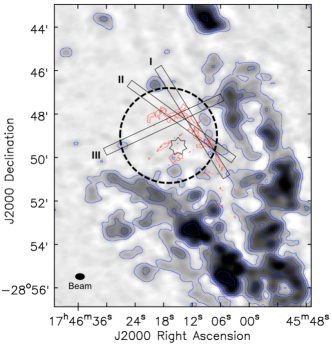
Figure 10: Maximum intensity NH₃ (3,3) emission from ATCA (SWAG survey; $\sim$20″ resolution, bottom left corner; Ott et al., 2017) over a velocity range of 45$-$65 km s^-1, with blue contours showing 5, 15, 25, 50 & 125 $\times$ 20 mJy beam^-1 (rms level). The red contour represents the 24.5 GHz continuum emission (from Figure 2) above 0.5 mJy beam^-1 (10$\sigma$ level). The black dashed circle shows the proposed size and location of the M0.20$-$0.033 expanding shell (see Figure 9 and Section 5.2.1). The star shows the location of the Quintuplet cluster. The black boxes show the relative lengths (350″) and integrated widths (5″) of slices I$-$III in Figure 11.

5.2.2 Kinematic Properties of the M0.20$-$0.033 Expanding Shell

Using the geometry of an expanding shell, we can estimate the systemic velocity, $v_{sys}$, and expansion velocity, $v_{exp}$, (see Appendix A for more details). We will assume the gas distribution in Figure 6 delineates the right half of the ellipse (i.e., semi-major axis in Figure A.2, right). Therefore, we identify the dashed line at location ‘A,’ in Figure 6, as the midpoint of the chord. Thus, the semi-major axis of this ellipse (i.e., r$\cdot$cos$\theta$, where r=135″) has an angular length of $\sim$100″. We measure a minimum velocity ($v_{min}$) of 23$\pm$3 km s^-1 and a maximum velocity ($v_{max}$) of 83$\pm$3 km s^-1 at the midpoint of this chord, resulting $v_{sys}$ equal to 53$\pm$3 km s^-1. This $v_{sys}$ corresponds well to the velocity measured at the edge of the shell (52$\pm$3 km s^-1) in Figure 6. Using $v_{min}$ and $v_{max}$ for this chord, located at an angle $\theta$ of 42° from the origin, we estimate $v_{exp}$=40$\pm$3 km s^-1.

Next, we can look for consistency between predicted values for $v_{min}$ and $v_{max}$ and the values of the $v_{min}$ and $v_{max}$ velocities measured in the molecular gas on a slightly larger scale. We can compare predicted values for $v_{min}$ and $v_{max}$ (using $v_{sys}$ and $v_{exp}$ as above) with the distribution of velocities in the position-velocity diagram for the lower resolution ($\sim$2′ resolution) molecular gas data shown in Figure 8. The predicted values for $v_{min}$ range from 20$-$35 km s^-1 and for $v_{max}$ range from 75$-$90 km s^-1 for a range of angles, $\theta$, 30$-$60°. The $v_{min}$ and $v_{max}$ measured in Figure 8 along the northern region of the cloud (‘N’) are 20$-$40 km s^-1 and 75$-$85 km s^-1, respectively. These values are in good agreement with the predicted values, illustrating that the parameters we suggest for the expanding shell are consistent with the data.

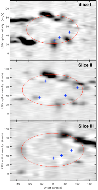
Figure 11: Position-velocity distribution of NH₃ (3,3) from ATCA of slices I$-$III (Figure 10). The red dashed ellipse shows the derived position-velocity distribution from Figure A.2 using a $v_{sys}$ of 53 km s^-1 and a $v_{exp}$ of 40 km s^-1 from Section 5.2.1. The chord length of the three different slices varies from 229″ (Slice I) to 255″ (Slice III). The blue crosses show the central velocity emission of the ionized gas at several locations across the slice (Section 5.3.2).

In order to further examine the position-velocity structure expected from an expanding shell (Figure A.2, right), we examine the ATCA data, as its angular resolution of $\sim$20″ provides a compromise between the VLA data (5″ resolution) and the Mopra data ($\sim$2′ resolution). Figure 10 shows the 45$-$65 km s^-1 molecular emission (i.e., roughly $\pm$10 km s^-1 from the suggested 53 km s^-1 systemic velocity, see discussion in Section 5.2.1), with the relative locations of: the M0.20$-$0.033 expanding shell, the Sickle H II region, and the Quintuplet cluster. We performed a position-velocity analysis on three slices (labeled slice I$-$III) across the M0.20$-$0.033 expanding shell as indicated by the black boxes in Figure 10. The three panels in Figure 11 (grayscale) show the position-velocity distribution of the observed molecular emission for each slice. These three panels were created using the CASA task IMPV, with a fixed length of 350″ and the center location of the chord. We measured the chord length for each slice and inferred the corresponding $v_{min}$ and $v_{max}$ of the ellipse, using the derived $v_{sys}$ and $v_{exp}$ from above. The dashed lines in Figure 11 show the resulting predicted ellipse, with the end points ($\pm$r$\cdot$cos$\theta$) corresponding to the edge of the shell (outlined in Figures 9 & 10). All three predicted ellipses generally follow the observed position-velocity distribution, indicating that our estimated systemic and expansion velocities are consistent with the observed emission. We conclude that the position-velocity structure supporting an expanding shell in the MC M0.20$-$0.033 is present in all of our observations that represent a range of spatial scales (from the high-resolution VLA data to the single-dish Mopra data).

5.2.3 Age and Orbital Stream of the M0.20$-$0.033 Expanding Shell

Using the assumption that the time derivative of $v_{exp}$ is zero, we can estimate an upper limit on the age of the shell ($t_{age}$=1.3$\times$10⁵ yr). The age and expansion velocity (40 km s^-1) of the M0.20$-$0.033 expanding shell are comparable with properties of other molecular shells in the GC (0.7$-$1.5$\times$10⁵ yr, and $\sim$20$-$30 km s^-1; Tsuboi et al., 1997; Oka et al., 2001a; Tsuboi et al., 2009). These molecular shells are all located within the inner 100 pc of the GC and are thought to be the result of several supernovae or a few hypernovae.

The central velocities detected in M0.10$-$0.08 (Section 5.1.2) are consistent with the derived systemic velocity of the M0.20$-$0.033 expanding shell (53 km s^-1). The consistency between the systemic velocities of these two clouds further supports our argument that these clouds are physically connected. If these two clouds are physically connected (i.e., on the same orbital stream) then the Doppler shifted velocities detected in M0.20$-$0.033 might be the result of a perturbation by the expanding shell. The perturbation in this stream might be the result of the Quintuplet cluster, which is $\sim$30″ (1.2 pc in projection) from the center of the M0.20$-$0.033 expanding shell (Figure 10). The expansion velocity of the M0.20$-$0.033 expanding shell is also consistent with velocities from wind-blown bubbles around massive clusters (e.g., Dent et al., 2009), indicating that this massive cluster might be the driving force behind the expanding shell.

The proposed interaction between the Quintuplet cluster and the expanding shell is consistent with the location of the cluster in the Kruijssen et al. (2015) orbital model. Based on the velocity of the Quintuplet cluster ($\sim$90$-$100 km s^-1; Stolte et al., 2014), Kruijssen et al. (2015) suggest that the cluster is also located on the near side of the GC (stream 1). In addition, our observations help to support the conclusions of Stolte et al. (2014), who argue that the parent cloud of the Quintuplet cluster is not on a circular orbit around the GC, but rather a non-circular orbit, such as the Kruijssen et al. (2015) orbital streams.

5.3 The Quintuplet cluster: Driving Force Behind the Expanding Shell?

The massive Quintuplet star cluster ($\sim$10^50.9 photons s^-1, age: 4.8$\pm$1.1 Myr; Figer et al., 1999a; Schneider et al., 2014) has a large population of massive stars (OB supergiants) and several unusual types of Wolf-Rayet stars. In total, this cluster is capable of ionizing the edge of the nearby ($\sim$1′; 2.3 pc in projection) M0.20$-$0.033 MC, producing the Sickle H II region (2.8$\times$10⁴⁹ photons s^-1, 240 M_⊙; Lang et al., 1997). In addition, radio detections of a number of the most powerful stellar winds from this cluster have been detected by Lang et al. (2005) and the collective winds are likely to be influencing the surrounding ISM. In order to determine whether the cluster is capable of driving the expansion, we compare the radiative momentum of the cluster ($\textrm{p}_{rad}$) to the momentum of the expanding shell (p_shell). Since the radiative and wind energy of the cluster can be lost by cooling processes and dissipated in shocks the conserved momentum, which cannot be dissipated, provides the most informative comparison.

Stellar clusters inject momentum into the surrounding ISM through a combination of radiation and winds (which are radiation driven). Radiative momentum from a cluster is injected into the surrounding ISM at a rate of $\dot{\textrm{p}}_{rad}$$\sim$$\epsilon$L_bol/c, where $\epsilon$ is the fraction of the radiation absorbed by the ISM (or covering factor; i.e., $\epsilon$$\leq$1). We assume $\epsilon$=0.5 based on the distribution of molecular gas in Figure 9, which shows an open cavity in the emission. We will also assume the bolometric luminosity of the Quintuplet cluster (L_bol=10⁸ L_⊙; Lang et al., 2005) is constant over the lifetime of the expanding shell: $t_{age}$. Therefore, the total momentum ($\textrm{p}_{rad}$=$\epsilon$$\dot{\textrm{p}}_{rad}$$t_{age}$) injected into the ISM by the Quintuplet cluster is 6.6$\times$10⁴ M_⊙ km s^-1.

Estimations of the molecular gas mass in M0.20$-$0.033 range from 0.6 to 1.3$\times 10^{5}$ M_⊙ (Serabyn & Guesten, 1991; Tsuboi et al., 2011). However, both of these mass estimates only account for the low-velocity molecular component. Therefore, the total mass of M0.20$-$0.033 would be twice these estimates, assuming the high-velocity molecular component has roughly the same amount of molecular gas. However, the area over which this mass is derived is approximately twice the size of the shell. Thus, we will assume the mass of the shell is M$\simeq$1$\times$10⁵ M_⊙, for the momentum calculation, with a $v$=$v_{exp}$. Therefore, the momentum of the expanding shell is $\sim$4$\times$10⁶ M_⊙ km s^-1.

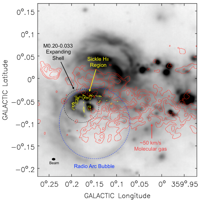
Figure 12: 21 $\mu$m MSX emission (Band E; greyscale, 18$\farcs$3 resolution) from Price et al. (2001). The blue dashed circle outlines the Simpson et al. (2007) Radio Arc bubble (see their Figure 1, right). The black dashed circle shows the M0.20$-$0.033 expanding shell (see Section 5.2.1). The red contours represent the 45$-$65 km s^-1 molecular emission at 5, 20 & 80 $\times$ 20 mJy beam^-1 (from Figure 10; $\sim$20″ resolution, bottom left corner). The yellow contour shows the 10$\sigma$ level of the 24.5 GHz radio continuum (Figure 2).

Clearly, the Quintuplet cluster alone does not have enough radiative momentum to drive the expansion. An additional source of momentum is needed to produce the observed expanding shell. This additional momentum could be in the form of supernova explosions. Given the age of the Quintuplet cluster (4.8$\pm$1.1 Myr) and the large number of evolved massive stars (Figer et al., 1999a), there is a high probability that some stars in the cluster have undergone a supernova explosion. The momentum injected by a single supernova into the surrounding ISM is $\textrm{p}_{sn}$=$\epsilon$M${}_{sn}v_{sn}$, where M_sn is the total ejecta mass and $v_{sn}$ is the initial blast wave expansion velocity. We will again assume a covering factor of $\epsilon$=0.5, since the molecular emission in Figure 9 shows an half-open cavity. Thus, $\textrm{p}_{sn}$$\sim$1.3$\times$10⁵ M_⊙ km s^-1 assuming a $v_{sn}$$\sim$10⁴ km s^-1 and M_sn$\sim$25 M_⊙. Therefore, approximately 30 supernovae (or a few hypernovae, M_sn$>$100 M_⊙) are needed to produce the expanding molecular shell detected. The production of this molecular shell by a number of supernova explosions would be reminiscent of the hypothesized production of other molecular shells detected in the GC (Tsuboi et al., 1997; Oka et al., 2001a; Tsuboi et al., 2009).

5.3.1 Connection to the Radio Arc Bubble?

The connection between the Quintuplet cluster and the molecular shell echoes several previous studies of this region. The GC ‘Radio Arc bubble’ (Simpson et al., 2007) is a large (d$\sim$10′; 20 pc) infrared bubble, that is suggested to be due to the outflow of matter and energy from the Quintuplet cluster. Figure 12 shows the relative location of the M0.20$-$0.033 expanding shell compared to the Radio Arc bubble presented in Simpson et al. (2007). The north and northeastern Galactic rim of the Radio Arc bubble coincide with the north and northeastern Galactic rim of the M0.20$-$0.033 expanding shell. Additionally, there is relatively bright 21 $\mu$m emission located $\sim$1′ inside the eastern Galactic rim of the M0.20$-$0.033 expanding shell. The southwest Galactic side of the Radio Arc bubble, however, extends $\sim$6′ ($\sim$15 pc) past the edge of the M0.20$-$0.033 expanding shell (see Figure 12) and is much fainter than emission detected near the M0.20$-$0.033 expanding shell.

We propose that the southwest side of the Radio Arc bubble corresponds to directions in which matter and energy flowing out of the cluster have encountered the least resistance (i.e., a relatively low-density ISM) and have broken out of the smaller region confined by molecular clouds. The circular structure of the Radio Arc bubble is well preserved towards the southern and western sides (Simpson et al., 2007, their Figure 1) indicating a weak interaction with the ambient ISM. This idea of a larger evacuated region has been evoked in the literature, as blown out (or broken) bubbles are quite common in the Galaxy and are detected in 38% of the 322 bubbles sampled by Churchwell et al. (2006). The velocities measured along this southwest rim of the Radio Arc bubble are consistent with velocities in the low-velocity molecular component (22$-$26 km s^-1, positions 10$-$12 in Simpson et al., 2007). Therefore, if the Radio Arc bubble is associated with the M0.20$-$0.033 expanding shell, then the bubble emission is predicted to be located on the near side of the region. Additionally, this breakout hypothesis might also account for the lack of emission in the low-velocity molecular component along regions of our shell (e.g., slice III in Figure 11) and in the single-dish observations by Serabyn & Guesten (1991).

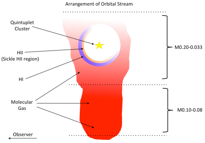
Figure 13: Schematic depicting our suggested arrangement of molecular components in the orbital stream (stream 1; Kruijssen et al., 2015), connecting M0.20$-$0.033 to M0.10$-$0.08 as discussed in Section 5.3. The molecular gas is shown in red, the H I gas is in purple, and the ionized gas is in orange. The yellow star shows the location of the Quintuplet cluster.

Hot X-ray emission is present inside the Radio Arc bubble (Ponti et al., 2015). Ponti et al. (2015) suggest that the hot gas inside this bubble is the combined result of winds from massive stars in the Quintuplet cluster and multiple supernovae explosions. This theory is consistent with our momentum calculations for the M0.20$-$0.033 expanding shell, which indicate that multiple supernovae are required to produce the shell.

5.3.2 The Sickle H II Region: an Inner Ionized Layer

As originally proposed by Serabyn & Guesten (1991) and Lang et al. (1997), and supported by our observations here, the Sickle H II region appears to be the ionized edge of the M0.20$-$0.033 MC by the Quintuplet cluster. This orientation of the ionizing cluster, H II region, and MC is consistent with predicted models of expanding shells produced by star clusters (Weaver et al., 1977; Dent et al., 2009). Figure 13 shows a possible arrangement of the interstellar and stellar components in the Radio Arc region where the Sickle H II region represents an inner ionized layer between the cluster and the cloud. The bent morphology of the Sickle H II region and location inside the M0.20$-$0.033 expanding shell (Figure 10), supports this suggestion. Additionally, 21 $\mu$m dust emission (MSX Band E; Price et al., 2001) is also detected $\sim$1′ inside the eastern Galactic rim of the M0.20$-$0.033 expanding shell (see Figure 12). Further, this relatively bright dust emission closely follows the Sickle H II region. Although no velocity information is obtained from these MSX observations, warm dust is known to be associated with H II regions (Paladini et al., 2012). While the morphology of the thermal radio continuum and warm dust support the hypothesis of an inner ionized gas layer, our VLA data can reveal some additional position velocity information. We can examine the distribution of ionized gas in position-velocity space along the same slices (where we have data from the Sickle H II region) as in Figure 11.

Given the proposed arrangement in Figure 13, we would expect to see that the velocities of the ionized gas would have values similar to the proposed position-velocity distribution for the expanding molecular shell (shown by the red dashed ellipses in Figure 11). The blue crosses in Figure 11 show the approximate central velocity of the ionized gas (estimated to within 5 km s^-1) at several locations along the respective slice. In nearly all cases, the values for the velocity of the ionized gas along slices I$-$III are close to the predictions for the velocities of expanding molecular shell. For example, the lowest ionized gas emission detected in slices I$-$III are located towards the predicted center of the shell, with values closer to the systemic velocity near the edge of the shell (Figure 11). This distribution supports the idea that the ionized gas is associated with the molecular shell.

Slices I$-$III in Figure 11 indicate that most of the ionized gas in the Sickle H II region have velocities lower than the systemic velocity of the M0.20$-$0.033 expanding shell ($v$ $\leq$ 53 km s^-1; Figures 11). These low velocities of the ionized gas are comparable with velocities detected in the low-velocity molecular component (e.g., see Figure 6), indicating the two components are physically connected. The similar velocities between most of the ionized gas and the low-velocity molecular component further suggests that the ionized gas is located on the nearside of the molecular shell. This orientation of components is consistent with the H I observations from Lang et al. (2010) (see Section 5.2). Additionally, the correlation between most of the ionized gas and low-velocity molecular component is consistent with the analysis in Serabyn & Guesten (1991) and Lang et al. (1997).

While most of the detected ionized gas emission is associated with the low-velocity component, we also detect relatively bright ionized emission from a high velocity clump ($\sim$75 km s^-1) that is located in the Sickle H II pillars (see Figure 4). Slice II in Figure 11 further shows that the location of this clump in position-velocity space correlates to molecular emission in the high-velocity component. The detection of ionized gas correlated with the high-velocity component supports our analysis that both molecular components of M0.20$-$0.033 are physically associated with the Quintuplet cluster. Thus, the distribution of the molecular and ionized gas, in position-velocity space, further supports our suggestion that the ionized gas is an inner layer between the cluster and cloud, as illustrated in Figure 13.

Even though little ionized gas is detected in the high-velocity component (see Figure 11), the results of Martín et al. (2008) support the hypothesis that the high-velocity component is associated with the Quintuplet cluster. They observed low HNCO/¹³CS abundance ratios in both velocity components, compared to other regions in the GC, and they therefore argue that both velocity components have photodissociation regions (PDRs). These low abundance ratios are typically found in regions around massive star clusters as the HCNO molecule is destroyed in strong UV radiation fields. Martín et al. (2008) find a factor of 3 difference in the abundance ratios between the low- and high-velocity components, with the high-velocity component having a higher value. They attribute this difference to a slight offset in the physical distance of the two components to the ionizing source, concluding that the low-velocity component is physically closer to the Quintuplet cluster. These findings are consistent with our results of the ionized gas distribution, which show considerably less ionized emission in the high-velocity component than in the low-velocity component.

The suggestion that the Sickle H II region is an inner ionized layer on the M0.20$-$0.033 expanding shell is also supported by the data of Langer et al. (2017). They observed [CII] towards the GC and argue that the [CII] emission within the inner 0$\fdg$25 of the GC is from highly ionized gas. Additionally, Figure 7 in Langer et al. (2017) shows an elliptical ring in position-velocity space at the Radio Arc region (e.g., Figure 1, inset). The velocity of the [CII] emission in this region range from 20 to 80 km s^-1 on both sides of the position-velocity ellipse. This range of velocities detected in the ionized gas emission (Langer et al., 2017) are consistent with the molecular gas velocities detected in this study. This elliptical ring in the [CII] emission is located in position-velocity space between streams 1 and 3 in the Kruijssen et al. (2015) orbital model and overlaps with molecular emission from both velocity components. As [CII] is also a known tracer of PDRs, the distribution of [CII] in Langer et al. (2017) is consistent with the results from Martín et al. (2008), who argue that both velocity components of M0.20$-$0.033 contain evidence of PDRs. Therefore, the consistency in the location and velocities of [CII] and the molecular gas indicates an inner PDR region ([CII]) between the cluster and molecular gas, as depicted in Figure 13.

The presence of ionized gas, most likely on the inside of the shell, may help to explain the lack of molecular emission detected towards the north-eastern side of the molecular shell (Figure 10). The lack of molecular emission near the eastern side is also evident in single-dish observations by Serabyn & Guesten (1991) (see their Figure 2). However, as stated in Section 5.2.1, there is molecular emission towards the north-eastern side of the shell at slightly lower and higher velocities (see the 40$-$50 & 60$-$70 km s^-1 panels in Figure 9). Ionized gas emission is detected on the north-eastern Galactic side of the Sickle H II region (i.e., the Sickle H II pillars) at velocities around 50 km s^-1 (see Figure 4, bottom right). The central velocities of the ionized gas in this region are comparable to the systemic velocities of M0.10$-$0.08 and the M0.20$-$0.033 expanding shell. The spectral profiles of the ionized and molecular gas lines in Figure 5, region A, also support this suggestion. The profile of the ionized gas emission in the Sickle H II pillars shows an intermediate-velocity that bridges the velocity space between the two molecular components (see Section 5.1.1).

The potential age we derive for the M0.20$-$0.033 expanding shell (1.3$\times$10⁵ yr; Section 5.2.3) is also comparable to the timescales needed for pillar formation by ionizing radiation from a single O-type star (2$-$4$\times$10⁵ yrs; Freyer et al., 2003; Mackey & Lim, 2010; Stolte et al., 2014). In conclusion, the morphological, chemical, and kinematic features detected in this region support a model in which the Sickle H II region represents a foreground inner layer between the M0.20$-$0.033 expanding molecular shell and the Quintuplet cluster.

6 Conclusions

We present high-resolution (5″) radio observations made with the VLA of molecular (NH₃) and ionized gas (H64$\alpha$ and H63$\alpha$ radio recombination lines) in the Radio Arc region of the Galactic center. This paper focuses on the region around M0.20$-$0.033, the Sickle H II region, and the Quintuplet cluster, but also addresses their physical relationship to other molecular clouds in the region (e.g., M0.10$-$0.08). These high-resolution observations were compared with intermediate-resolution ($\sim$20″; ATCA) and low-resolution ($\sim$2′; Mopra) observations to yield the following conclusions:

(1) The low and high-velocity components in M0.20-0.033 are physically connected in position-velocity space toward the Galactic western side of the cloud, via an intermediate-velocity component (around 55 km s^-1). The connection between both velocity components is also observed on larger scales ($\sim$2′; $\sim$5 pc).

(2) In the orbital model proposed by Kruijssen et al. (2015), the kinematics of M0.20$-$0.033 place this complex on their stream 1. The physical connection in position-velocity space between M0.20$-$0.033 and M0.10$-$0.08 is consistent with this suggestion.

(3) We interpret the morphology and kinematic structure of M0.20$-$0.033 as an expanding shell. In this scenario, the low-velocity component in the ionized and molecular gas lies on the foreground side of the shell and the high-velocity component on the backside.

(4) The M0.20$-$0.033 expanding shell has a systemic velocity of 53 km s^-1, comparable to the central velocities detected in M0.10$-$0.08, and a radius of $r$=135″ (5.2 pc). The expansion velocity of the shell is 40 km s^-1, implying an upper limit on the age of $\sim$1.3$\times$10⁵ years.

(5) The origin of the proposed expanding shell is located near the Quintuplet cluster, which is also on stream 1. The connection between the Quintuplet cluster and the M0.20$-$0.033 expanding shell is supported by our momentum calculations (Section 5.3). These show that $\sim$30 supernovae, or a few hypernovae, are needed to power the shell. The expansion of the M0.20$-$0.033 shell by multiple supernovae is analogous with other molecular shells in the GC.

7 Acknowledgements

The research presented in this paper was supported by grants from the National Science Foundation (no. AST-0907934 and no. AST-15243000) and the NASA Iowa Space Grant Consortium (ISCG) 2015-2016 fellowship. Support for this work was also provided by the NSF through the Grote Reber Fellowship Program administered by Associated Universities, Inc./National Radio Astronomy Observatory. We would also like to thank Diederik Kruijssen, Miguel Requena-Torres, Allison Costa, and Sarah Sadavoy for their helpful discussion on this work. We would also like to thank the anonymous referee for reviewing this work.

Appendix A Geometry of an Expanding Shell

A.1 Projected Radial Size of an Expanding Shell

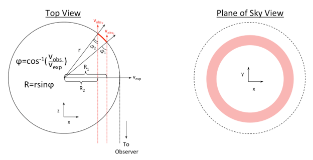
Figure A.1: (left): Schedmatic illustrating the line-of-sight geometry of a uniformly expanding shell, where v_obs is the observed doppler-shifted velocity, for an expansion velocity of v_exp, and R is the projected radius of the shell at v_obs. The two equations in left show the calculation of R using v_obs and v_exp. (right): shows the plane of sky orientation of left.

The apparent radial size of an expanding shell, projected in the sky, changes as a function of the observed Doppler-shifted velocity: v_obs. Figure A.1 (left) shows the line of sight geometry of an expanding shell viewed at different Doppler-shifted velocities. In this schematic we are assuming that (1) we are in the reference frame of the expanding shell, (2) the shell is thin compared to the radius ($\Delta$r$<<$r), and (3) the shell is expanding isotropically in all directions. Under these assumptions, v_obs changes as a function of $\varphi$, where $\varphi$ is the angle normal to the radial expansion vector: v_exp. The observed location of emission with v_obs (R in Figure A.1, left), is also dependent on the sine of $\varphi$, for a fixed shell radius: r. For observed Doppler-shifted emission between v_obs1 and v_obs2, the projected radial size of the shell would range from R₁ to R₂ (Figure A.1, left).

Figure A.1 (right) shows the plane of sky orientation of the schematic depicted on the left. The black dashed circle represents the radial size of the shell at the systemic velocity (i.e., v_obs=0; see black dashed line in Figure A.1, left). The red shaded annulus shows the projected size of the two Doppler-shifted velocities from Figure A.1, left. When viewed in the plane of the sky, gas between these velocities would form an annulus with an outer radius, R₁, and inner radius, R₂ (e.g., Figure A.1, right).

A.2 An Expanding Shell in Position-Velocity Space

An expanding shell is known to produce an elliptical distribution in position-velocity space. However, because the expanding shell is viewed in 2D space, the line-of-sight expansion velocity detected is dependent on the $x$$-$$y$ coordinate of the shell in the plane of the sky. Figure A.2 (left) illustrates an observed shell in the plane of the sky that has radius, $r$, expansion velocity, $v_{exp}$, and systemic velocity, $v_{sys}$. The red and blue dotted lines in Figure A.2 (left) represent potential ‘slices’ across the shell. Figure A.2 (right) shows a position-velocity schematic of these two example slices. The position axis (Figure A.2, right) corresponds to the length across the shell (Figure A.2 left), or chord length, where 0 denotes the midpoint of the chord. The total length of any chord across the shell is equal to the major axis of the ellipse (i.e., 2r$\cdot$cos$\theta$). The blue slice (hereafter, slice 1) corresponds to a chord length equal to the diameter of the shell (i.e., $\theta$=0). The measured minimum and maximum velocities for slice 1 would reflect the expansion velocity ($v_{exp}$) as the vector is oriented parallel to our line-of-sight. The red slice (hereafter, slice 2) is located at some position angle, $\theta$, above (or below) a slice through the origin (i.e., slice 1). At the midpoint of slice 2, the expansion velocity vector is also at an angle $\theta$ from our line-of-sight. Therefore the maximum Doppler shift of the gas we would detect along slice 2 is dependent on the cosine of the angle. For a uniformly expanding spherical shell, this schematic can be applied to any slice across the shell.

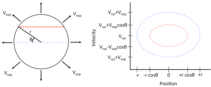
Figure A.2: Schematic depicting a translation of slices across an expanding shell into position-velocity space. (left): illustration of the expanding shell, with a systemic velocity of $v_{sys}$, an expansion velocity of $v_{exp}$, and radius $r$. (right): position-velocity diagram of an expanding shell for the two different cuts across the shell on the left.

References

- Bally et al. (1987) Bally, J., Stark, A. A., Wilson, R. W., & Henkel, C. 1987, ApJS, 65, 13
- Boehle et al. (2016) Boehle, A., Ghez, A. M., Schödel, R., et al. 2016, ApJ, 830, 17
- Churchwell et al. (2006) Churchwell, E., Povich, M. S., Allen, D., et al. 2006, ApJ, 649, 759
- Dent et al. (2009) Dent, W. R. F., Hovey, G. J., Dewdney, P. E., et al. 2009, MNRAS, 395, 1805
- Figer et al. (1999a) Figer, D. F., McLean, I. S., & Morris, M. 1999a, ApJ, 514, 202
- Figer et al. (1999b) Figer, D. F., Morris, M., Geballe, T. R., et al. 1999b, ApJ, 525, 759
- Freyer et al. (2003) Freyer, T., Hensler, G., & Yorke, H. W. 2003, ApJ, 594, 888
- Handa et al. (2006) Handa, T., Sakano, M., Naito, S., Hiramatsu, M., & Tsuboi, M. 2006, ApJ, 636, 261
- Hüttemeister et al. (1993) Hüttemeister, S., Wilson, T. L., Bania, T. M., & Martin-Pintado, J. 1993, Astronomy and Astrophysics (ISSN 0004-6361), 280, 255
- International Consortium Of Scientists (2011) International Consortium Of Scientists. 2011, CASA: Common Astronomy Software Applications, Astrophysics Source Code Library, , , ascl:1107.013
- Krieger et al. (2017) Krieger, N., Ott, J., Walter, F., Kruijssen, J. M. D., & Beuther, H. 2017, in IAU Symposium, Vol. 322, The Multi-Messenger Astrophysics of the Galactic Centre, ed. R. M. Crocker, S. N. Longmore, & G. V. Bicknell, 160–161
- Kruijssen et al. (2015) Kruijssen, J. M. D., Dale, J. E., & Longmore, S. N. 2015, MNRAS, 447, 1059
- Lang et al. (2010) Lang, C. C., Goss, W. M., Cyganowski, C., & Clubb, K. I. 2010, ApJS, 191, 275
- Lang et al. (1997) Lang, C. C., Goss, W. M., & Wood, O. S. 1997, ApJ, 474, 275
- Lang et al. (2005) Lang, C. C., Johnson, K. E., Goss, W. M., & Rodríguez, L. F. 2005, AJ, 130, 2185
- Langer et al. (2017) Langer, W. D., Velusamy, T., Morris, M. R., Goldsmith, P. F., & Pineda, J. L. 2017, A&A, 599, A136
- Lau et al. (2014) Lau, R. M., Herter, T. L., Morris, M. R., & Adams, J. D. 2014, ApJ, 785, 120
- Longmore et al. (2013) Longmore, S. N., Bally, J., Testi, L., et al. 2013, MNRAS, 429, 987
- Ludovici et al. (2016) Ludovici, D. A., Lang, C. C., Morris, M. R., et al. 2016, ApJ, 826, 218
- Mackey & Lim (2010) Mackey, J., & Lim, A. J. 2010, MNRAS, 403, 714
- Martín et al. (2008) Martín, S., Requena-Torres, M. A., Martín-Pintado, J., & Mauersberger, R. 2008, ApJ, 678, 245
- Mauerhan et al. (2010) Mauerhan, J. C., Morris, M. R., Cotera, A., et al. 2010, ApJ, 713, L33
- Mauersberger et al. (1986) Mauersberger, R., Henkel, C., Wilson, T. L., & Walmsley, C. M. 1986, A&A, 162, 199
- Mills & Morris (2013) Mills, E. A. C., & Morris, M. R. 2013, ApJ, 772, 105
- Molinari et al. (2011) Molinari, S., Bally, J., Noriega-Crespo, A., et al. 2011, ApJ, 735, L33
- Oka et al. (2001a) Oka, T., Hasegawa, T., Sato, F., Tsuboi, M., & Miyazaki, A. 2001a, PASJ, 53, 779
- Oka et al. (2001b) Oka, T., Hasegawa, T., Sato, F., et al. 2001b, ApJ, 562, 348
- Ott et al. (2017) Ott, J., Meier, D. S., Krieger, N., & Rickert, M. 2017, in IAU Symposium, Vol. 322, The Multi-Messenger Astrophysics of the Galactic Centre, ed. R. M. Crocker, S. N. Longmore, & G. V. Bicknell, 143–144
- Paladini et al. (2012) Paladini, R., Umana, G., Veneziani, M., et al. 2012, ApJ, 760, 149
- Ponti et al. (2015) Ponti, G., Morris, M. R., Terrier, R., et al. 2015, MNRAS, 453, 172
- Price et al. (2001) Price, S. D., Egan, M. P., Carey, S. J., Mizuno, D. R., & Kuchar, T. A. 2001, AJ, 121, 2819
- Purcell et al. (2012) Purcell, C. R., Longmore, S. N., Walsh, A. J., et al. 2012, MNRAS, 426, 1972
- Schneider et al. (2014) Schneider, F. R. N., Izzard, R. G., de Mink, S. E., et al. 2014, ApJ, 780, 117
- Serabyn & Guesten (1991) Serabyn, E., & Guesten, R. 1991, A&A, 242, 376
- Serabyn & Morris (1994) Serabyn, E., & Morris, M. 1994, ApJ, 424, L91
- Simpson et al. (2007) Simpson, J. P., Colgan, S. W. J., Cotera, A. S., et al. 2007, ApJ, 670, 1115
- Stolte et al. (2014) Stolte, A., Hußmann, B., Morris, M. R., et al. 2014, ApJ, 789, 115
- Tsuboi et al. (2009) Tsuboi, M., Miyazaki, A., & Okumura, S. K. 2009, PASJ, 61, 29
- Tsuboi et al. (2011) Tsuboi, M., Tadaki, K.-I., Miyazaki, A., & Handa, T. 2011, PASJ, 63, 763
- Tsuboi et al. (1997) Tsuboi, M., Ukita, N., & Handa, T. 1997, ApJ, 481, 263
- Walsh et al. (2008) Walsh, A. J., Lo, N., Burton, M. G., et al. 2008, PASA, 25, 105
- Walsh et al. (2011a) Walsh, A. J., Breen, S. L., Britton, T., et al. 2011a, in EAS Publications Series, Vol. 52, EAS Publications Series, ed. M. Röllig, R. Simon, V. Ossenkopf, & J. Stutzki, 135–138
- Walsh et al. (2011b) Walsh, A. J., Breen, S. L., Britton, T., et al. 2011b, MNRAS, 416, 1764
- Wang et al. (2010) Wang, Q. D., Dong, H., Cotera, A., et al. 2010, MNRAS, 402, 895
- Weaver et al. (1977) Weaver, R., McCray, R., Castor, J., Shapiro, P., & Moore, R. 1977, ApJ, 218, 377
- Yusef-Zadeh & Morris (1987) Yusef-Zadeh, F., & Morris, M. 1987, AJ, 94, 1178
- Zylka et al. (1992) Zylka, R., Guesten, R., Henkel, C., & Batrla, W. 1992, A&AS, 96, 525