An ensemble algorithm for numerical solutions to deterministic and random parabolic PDEs

Abstract

In this paper, we develop an ensemble-based time-stepping algorithm to efficiently find numerical solutions to a group of linear, second-order parabolic partial differential equations (PDEs). Particularly, the PDE models in the group could be subject to different diffusion coefficients, initial conditions, boundary conditions, and body forces. The proposed algorithm leads to a single discrete system for the group with multiple right-hand-side vectors by introducing an ensemble average of the diffusion coefficient functions and using a new semi-implicit time integration method. The system could be solved more efficiently than multiple linear systems with a single right-hand-side vector. We first apply the algorithm to deterministic parabolic PDEs and derive a rigorous error estimate that shows the scheme is first-order accurate in time and is optimally accurate in space. We then extend it to find stochastic solutions of parabolic PDEs with random coefficients and put forth an ensemble-based Monte Carlo method. The effectiveness of the new approach is demonstrated through theoretical analysis. Several numerical experiments are presented to illustrate our theoretical results.

65C05, 65C20, 65M60

1 Introduction

In many application problems involving numerical simulations of PDEs, one is not interested in a single simulation, but a number of simulations with different computational settings such as distinct initial condition, boundary conditions, body force, and physical parameters. For instance, data assimilation methods used in meteorology, such as the ensemble Kalman filter [14], run a numerical weather model forward for many times by perturbing initial conditions and uncertain parameters. The ensemble of outputs is then used to update not only the forecast, but also the covariance matrix. Similarly, when a random sampling method is used in uncertainty quantification, a model is run forward for a large number of times at the selected parameter sample values in order to collect outputs and determine the underlying statistical information [7]. Such a group of simulations is computationally expensive, especially, when the forward simulation is of a large scale.

Aiming at developing a fast algorithm for such applications, an ensemble time-stepping algorithm was proposed in [12], where a group of size $J$ Navier-Stokes equations (NSE) with different initial conditions and forcing terms is simulated. All solutions are found by solving a single linear system with one shared coefficient matrix and $J$ right-hand-side (RHS) vectors at each time step. Thus, it reduces the storage requirements and computational cost for the group of simulations. The algorithm is first-order accurate in time, which was extended to higher-order accurate schemes in [9, 10]. For high Reynolds number incompressible flows, ensemble regularization methods were developed in [9, 13, 21], and a turbulence model based on ensemble averaging was developed in [11]. The ensemble algorithm has also been extended to simulate MHD flows in [17] and to the reduced-order modeling setting in [4, 5]. For parametrized flows, the ensemble algorithms were developed in [6] for multiple numerical simulations subject to not only different initial condition, boundary conditions and body force, but also physical parameters. It is worth mentioning that the ensemble method is only applied to problems with constant physical parameters so far.

In this paper, we consider a group of numerical solutions to second-order parabolic PDEs. We first develop an ensemble algorithm for deterministic problems, in which the physical parameter—diffusion coefficient—is a function of space and time; and then extend the method to stochastic problems. To our knowledge, this is the first time that an ensemble scheme is derived for problems with non-constant parameters and is further applied to PDEs with random coefficients.

The initial boundary value problem we consider is as follows.

(1) $$\left\{\begin{aligned} u_{t}-\nabla\cdot[a({\bf x},t)\nabla u]&=f({\bf x},t),&\text{ in }D\times(0,T){,}\\ u({\bf x},t)&=g({\bf x},t),\qquad&\text{ on }\partial D\times(0,T){,}\\ u({\bf x},0)&=u^{0}({\bf x}),&\text{ in }D{,}\end{aligned}\right.$$

where $D$ is a bounded Lipschitz domain in $\mathbb{R}^{d}$ for $d=1,2,3$, the diffusion coefficient $a({\bf x},t)\in L^{2}(W^{1,\infty}(D);0,T)$, body force $f({\bf x},t)\in L^{2}(H^{-1}(D);0,T)$, initial condition $u^{0}({\bf x})\in H_{0}^{1}(D)\cap H^{l+1}(D)$ with $l\geq 1$.

We consider the setting in which one needs to run a group of simulations. Each of these simulations is subject to independent initial and boundary conditions, body force and diffusion coefficient. Suppose the ensemble of simulations includes $J$ independent members, in which the $j$-th member satisfies:

(2) $$\left\{\begin{aligned} u_{j,t}-\nabla\cdot[a_{j}({\bf x},t)\nabla u_{j}]&=f_{j}({\bf x},t),&\text{ in }D\times(0,T){,}\\ u_{j}({\bf x},t)&=g_{j}({\bf x},t),&\text{ on }\partial D\times(0,T){,}\\ u_{j}({\bf x},0)&=u_{j}^{0}({\bf x}),&\text{ in }D{,}\end{aligned}\right.$$

for $j=1,2,\ldots,J$. In general, when an implicit time stepping method is applied to the above system, the related discrete system would change as $j$ varies. As a result, one needs to solve $J$ linear systems at each time step. In order to improve its efficiency, we develop an ensemble-based time-stepping scheme. For illustrating the main idea, we first present the semi-discrete (in time) system.

For simplicity, we consider a uniform time partition on $[0,T]$ with the step size $\Delta t$. Denote by $u_{j}^{n}$, $a_{j}^{n}$ and $f_{j}^{n}$ the functions $u_{j}$, $a_{j}$ and $f_{j}$ evaluated at the time instant $t_{n}=n\Delta t$. Define the ensemble mean of the diffusion coefficient functions at time $t_{n}$ by

(3) $$\overline{a}^{n}:=\frac{1}{J}\sum\limits_{j=1}^{J}a_{j}({\bf x},t_{n}).$$

The new ensemble-based time stepping scheme reads, for $j=1,\ldots,J$:

(4) $$\frac{u_{j}^{n+1}-u_{j}^{n}}{{\Delta t}}-\nabla\cdot({\overline{a}^{n+1}}\nabla u_{j}^{n+1})-\nabla\cdot[(a_{j}^{n+1}-{\overline{a}}^{n+1})\nabla u_{j}^{n}]=f_{j}^{n+1}$$

with the same boundary and initial conditions as those in (2). Rearranging the equation gives

(5) $$\frac{1}{\Delta t}{u_{j}^{n+1}}-\nabla\cdot({\overline{a}}^{n+1}\nabla u_{j}^{n+1})=f_{j}^{n+1}+\frac{1}{\Delta t}{u_{j}^{n}}+\nabla\cdot[(a_{j}^{n+1}-{\overline{a}}^{n+1})\nabla u_{j}^{n}].$$

It is easy to see, after a spatial discretization, the coefficient matrix of the resulting linear system will be independent of $j$. This represents the key feature of the ensemble method, that is, the discrete systems associated with an ensemble of simulations share a unique coefficient matrix and only the RHS vectors vary among the ensemble members. Thus, when the considered problem has a small scale, one only needs to do LU factorization of the coefficient matrix once and use it to find the solutions of the group; when the problem is of a large scale, the proposed scheme together with the block Krylov subspace iterative methods will improve the efficiency of a number of numerical simulations (see, e.g. [20] and references therein).

The rest of this paper is structured as follows. In Section 2, we introduce some notations and mathematical preliminaries. In Section 3, we analyze the ensemble scheme (4) under a full discretization in both space and time, and prove its stability and convergence. In Section 4, we discuss the random parabolic equations and provide stability analysis and error estimations. Several numerical experiments are presented in Section 5, which illustrates the effectiveness of our proposed scheme on both deterministic and random parabolic problems. A few concluding remarks are given in Section 6.

2 Notations and preliminaries

Denote the $L^{2}(D)$ norm and inner product by $\|\cdot\|$ and $(\cdot,\cdot)$, respectively. Let $L^{\infty}(D)$ be the set of bounded measurable functions equipped with the norm $|v|_{\infty}:=\text{ess sup}_{{\bf x}\in D}|v|$. Denoted by $W^{s,q}(D)$ the Sobolev space of functions having generalized derivatives up to the order $s$ in the space $L^{q}(D)$, where $s$ is a nonnegative integer and $1\leq q\leq+\infty$. The equipped Sobolev norm of $v\in W^{s,q}(D)$ is denoted by $\|v\|_{W^{s,q}(D)}$. When $q=2$, we use the notation $H^{s}(D)$ instead of $W^{s,2}(D)$. As usual, the function space $H_{0}^{1}(D)$ is the subspace of $H^{1}(D)$ consisting of functions that vanish on the boundary of $D$ in the sense of trace, equipped with the norm $\|v\|_{H^{1}_{0}(D)}=\left(\int_{D}|\nabla v|^{2}\,d{\bf x}\right)^{1/2}$. When $s=0$, we shall keep the notation with $L^{q}(D)$ instead of $W^{0,q}(D)$. The space $H^{-s}(D)$ is the dual space of bounded linear functions on $H_{0}^{s}(D)$. A norm for $H^{-1}(D)$ is defined by $\|f\|_{-1}=\sup_{0\neq v\in H_{0}^{1}(D)}{(f,v)}/{\|\nabla v\|}.$

Stochastic functions have different structures. Let $(\Omega,\mathcal{F},P)$ be a complete probability space, where $\Omega$ is the set of outcomes, $\mathcal{F}\subset 2^{\Omega}$ is the $\sigma-$algebra of events, and $P:\mathcal{F}\rightarrow[0,1]$ is a probability measure. If $Y$ is a random variable in the space and belongs to $L_{P}^{1}(\Omega)$, its expected value is defined by

$$E[Y]=\int_{\Omega}Y(\omega)dP(\omega).$$

With the multi-index notation, $\alpha=(\alpha_{1},\ldots,\alpha_{d})$ is a $d$-tuple of nonnegative integers with the length $|\alpha|=\sum_{i=1}^{d}\alpha_{i}$. The stochastic Sobolev spaces $\widetilde{W}^{s,q}(D)=L^{q}_{P}(\Omega,W^{s,q}(D))$ containing stochastic function, $v:\Omega\times D\rightarrow R$, that are measurable with respect to the product $\sigma$-algebra $\mathcal{F}\bigotimes B(D)$ and equipped with the averaged norms $\|v\|_{\widetilde{W}^{s,q}(D)}=\left(E\left[\|v\|^{q}_{W^{s,q}(D)}\right]\right)^{1/q}=\left(E\left[\sum_{|\alpha\leq s|}\int_{D}|\partial^{\alpha}v|^{q}d{\bf x}\right]\right)^{1/q},1\leq q<+\infty$. Observe that if $v\in\widetilde{W}^{s,q}(D)$, then $v(\omega,\cdot)\in W^{s,q}(D)$ almost surely (a.s.) and $\partial^{\alpha}v(\cdot,{\bf x})\in L^{q}_{P}(\Omega)$ almost everywhere (a.e.) on the $D$ for $|\alpha|\leq s$. Whenever $q=2$, the above space is a Hilbert space, i.e., $\widetilde{W}^{s,2}(D)=\widetilde{H}^{s}(D)\simeq L^{2}_{P}(\Omega)\bigotimes H^{s}(D)$. In this paper, we consider the tensor product Hilbert space $H=\widetilde{L}^{2}(H^{1}_{0}(D);0,T)\simeq L^{2}_{P}(\Omega;H_{0}^{1}(D);0,T)$ endowed with the inner product $(v,u)_{H}\equiv E\left[\int_{0}^{T}\int_{D}\nabla v\cdot\nabla u\,d{\bf x}\,dt\right]$.

3 The ensemble scheme of deterministic parabolic equations

We first consider the deterministic parabolic equations and analyze the full discretization of the proposed ensemble scheme (4). For simplicity of presentation, we consider the problem with a homogeneous boundary condition, while the nonhomogeneous cases can be similarly analyzed incorporating the method of shifting (see Section 5.4 in [2]). Furthermore, we include numerical test cases with nonhomogeneous boundary conditions in Section 5.

Suppose the following two conditions are valid:

• There exists a positive constant $\theta$ such that, for any $t\in[0,T]$,

  (6) $$\min\limits_{{\bf x}\in{\overline{D}}}a({\bf x},t)\geq\theta;$$

• There exist positive constants $\theta_{-}$ and $\theta_{+}$ such that, for any $t\in[0,T]$,

  (7) $$\theta_{-}\leq|a_{j}({\bf x},t)-\overline{a}({\bf x},t)|_{\infty}\leq\theta_{+}.$$

Obviously, Condition (i) guarantees the uniform coercivity of the problem; Condition (ii) states that the distance from coefficient $a_{j}({\bf x},t)$ to the ensemble average $\overline{a}({\bf x},t)$ is uniformly bounded.

Let ${\mathcal{T}}_{h}$ be a quasi-uniform triangulation of the domain $D$, made of elements $K$, such that $\overline{D}=\bigcup_{K\in{\mathcal{T}}_{h}}\overline{K}$. Define the mesh size $h:=\max_{K\in\mathcal{T}_{h}}h_{K}$, where $h_{K}$ is the diameter of the element $K$. Denoted by $V_{h}$ the finite element space

$$V_{h}:=\{v\in H_{0}^{1}(D)\cap H^{l+1}(D);v|_{K}\text{ is a polynomial of degree }l,\forall K\in{\mathcal{T}}_{h}\}.$$

With the assumed uniform time partition on $[0,T]$ and set $N=T/\Delta t$, the fully discrete approximation of (4) is as follows: Find $u_{j,h}^{n+1}\in V_{h}$ satisfying, for $n=0,\ldots,N-1$ and $j=1,\cdots,J$ :

(8) $$\left(\frac{u_{j,h}^{n+1}-u_{j,h}^{n}}{\Delta t},v_{h}\right)+\left(\overline{a}^{n+1}\nabla u_{j,h}^{n+1},\nabla v_{h}\right) +\left((a_{j}^{n+1}-\overline{a}^{n+1})\nabla u_{j,h}^{n},\nabla v_{h}\right)$$

$$=\left(f_{j}^{n+1},v_{h}\right),\quad\forall\,v_{h}\in V_{h}$$

with the initial condition $u_{j,h}^{0}\in V_{h}$ satisfying $(u_{j,h}^{0},v_{h})=(u_{j}^{0},v_{h})$, $\forall\,v_{h}\in V_{h}$.

3.1 Stability and convergence

We first discuss the stability of the ensemble algorithm (8).

Theorem 3.1.

Suppose $f_{j}\in L^{2}(H^{-1}(D);0,T)$ and conditions (i) and (ii) are satisfied, the ensemble scheme (8) is stable provided that

(9) $$\theta>\theta_{+}.$$

Furthermore, the numerical solution to (8) satisfies

(10) $$\|u_{j,h}^{N}\|^{2}+\theta_{-}\Delta t\|\nabla u_{j,h}^{N}\|^{2}+(\theta-\theta_{+})\Delta t\sum_{n=1}^{N}\|\nabla u_{j,h}^{n}\|^{2}\leq C\Delta t\sum\limits_{n=1}^{N}\|f_{j}^{n}\|_{-1}^{2}$$

$$+C\Delta t\|\nabla u_{j,h}^{0}\|^{2}+\|u_{j,h}^{0}\|^{2},$$

where $C$ is a generic positive constant independent of $J$, $h$ and $\Delta t$.

Proof 3.2.

Taking $v_{h}=u_{j,h}^{n+1}$ in (8), we have

$$\frac{1}{\Delta t}(u_{j,h}^{n+1}-u_{j,h}^{n},u_{j,h}^{n+1})+(\overline{a}^{n+1}\nabla u_{j,h}^{n+1},\nabla u_{j,h}^{n+1}) +((a_{j}^{n+1}-\overline{a}^{n+1})\nabla u_{j,h}^{n},\nabla u_{j,h}^{n+1})$$

$$=(f_{j}^{n+1},u_{j,h}^{n+1}).$$

Multiplying both sides by $\Delta t$, and using the polarization identity and coercivity of $\overline{a}^{n+1}$, we get

(11) $$\frac{1}{2}\|u_{j,h}^{n+1}\|^{2}-\frac{1}{2}\|u_{j,h}^{n}\|^{2} +\frac{1}{2}\|u_{j,h}^{n+1}-u_{j,h}^{n}\|^{2}+\Delta t\,\theta\|\nabla u_{j,h}^{n+1}\|^{2}$$

$$\leq-\Delta t((a_{j}^{n+1}-\overline{a}^{n+1})\nabla u_{j,h}^{n},\nabla u_{j,h}^{n+1})+\Delta t(f_{j}^{n+1},u_{j,h}^{n+1}).$$

By the Cauchy-Schwarz and Young’s inequalities, we have, for some $\mu$, $\alpha>0$,

(12) $$\Delta t\left|((a_{j}^{n+1}-\overline{a}^{n+1})\nabla u_{j,h}^{n},\nabla u_{j,h}^{n+1})\right| \leq \Delta t{\left|a_{j}^{n+1}-\overline{a}^{n+1}\right|_{\infty}}\|\nabla u_{j,h}^{n}\|\|\nabla u_{j,h}^{n+1}\|$$

$$\leq \Delta t{\left|a_{j}^{n+1}-\overline{a}^{n+1}\right|_{\infty}}\left(\frac{1}{2\mu}\|\nabla u_{j,h}^{n}\|^{2}+\frac{\mu}{2}\|\nabla u_{j,h}^{n+1}\|^{2}\right)$$

and

(13) $$\Delta t|(f_{j}^{n+1},u_{j,h}^{n+1})|\leq\Delta t\|f_{j}^{n+1}\|_{-1}\|\nabla u_{j,h}^{n+1}\|\leq\frac{\Delta t}{4\alpha}\|f_{j}^{n+1}\|_{-1}^{2}+\alpha\Delta t\|\nabla u_{j,h}^{n+1}\|^{2}.$$

Substituting (12) and (13) into (11) and dropping the non-negative term $\frac{1}{2}\|u_{j,h}^{n+1}-u_{j,h}^{n}\|^{2}$, we get

$$\frac{1}{2}\left(\|u_{j,h}^{n+1}\|^{2}-\|u_{j,h}^{n}\|^{2}\right) + \Delta t\left[\theta-\alpha-\left(\frac{\mu}{2}+\frac{1}{2\mu}\right)\left|a_{j}^{n+1}-\overline{a}^{n+1}\right|_{\infty}\right]\|\nabla u_{j,h}^{n+1}\|^{2}$$

$$+ \frac{\Delta t}{2\mu}\left|a_{j}^{n+1}-\overline{a}^{n+1}\right|_{\infty}\left(\|\nabla u_{j,h}^{n+1}\|^{2}-\|\nabla u_{h}^{n}\|^{2}\right)\leq\frac{\Delta t}{4\alpha}\|f_{j}^{n+1}\|_{-1}^{2}.$$

Multiplying both sides by $2$, summing over $n$ from 0 to $N-1$ and taking $\mu=1$ yields

(14) $$\|u_{j,h}^{N}\|^{2} - \|u_{j,h}^{0}\|^{2}+2\Delta t\sum\limits_{n=0}^{N-1}\left(\theta-\alpha-\left|a_{j}^{n+1}-\overline{a}^{n+1}\right|_{\infty}\right)\|\nabla u_{j,h}^{n+1}\|^{2}$$

$$+ \Delta t\sum\limits_{n=0}^{N-1}\left|a_{j}^{n+1}-\overline{a}^{n+1}\right|_{\infty}\left(\|\nabla u_{j,h}^{n+1}\|^{2}-\|\nabla u_{j,h}^{n}\|^{2}\right)\leq\frac{\Delta t}{2\alpha}\sum\limits_{n=0}^{N-1}\|f_{j}^{n+1}\|_{-1}^{2}.$$

We then choose $\alpha=(\theta-{\left|a_{j}^{n+1}-\overline{a}^{n+1}\right|}_{\infty})/2$ and use the conditions (7) and (9), and obtain

$$\|u_{j,h}^{N}\|^{2}+\theta_{-}\Delta t\|\nabla u_{j,h}^{N}\|^{2}+(\theta-\theta_{+})\Delta t\sum_{n=0}^{N-1}\|\nabla u_{j,h}^{n+1}\|^{2}\leq{\frac{\Delta t}{\theta-\theta_{+}}}\sum\limits_{n=0}^{N-1}\|f_{j}^{n+1}\|_{-1}^{2}$$

$$+{\theta_{-}}\Delta t\|\nabla u_{j,h}^{0}\|^{2}+\|u_{j,h}^{0}\|^{2}.$$

This completes the proof.

Remark 3.3.

The stability condition (9) requires, for $\{a_{j}\}_{j=1}^{J}$, the deviation of $a_{j}$ from the ensemble average $\overline{a}$ to be less than the coercivity constant $\theta$. If this is not the case, one might divide the ensemble into smaller groups so that the stability condition holds in each of them and the algorithm is stable and applicable.

Next, we estimate the approximation error of the ensemble algorithm (8). We assume the exact solution of the PDEs is smooth enough, in particular,

$$u_{j}\in L^{2}(H_{0}^{1}(D)\cap H^{l+1}(D);0,T)\cap H^{1}(H^{l+1}(D);0,T)\cap H^{2}(L^{2}(D);0,T).$$

Theorem 3.4.

Let $u_{j}^{n}$ and $u_{j,h}^{n}$ be the solutions of equations (2) and (8) at time $t_{n}$, respectively. Assume $f_{j}\in L^{2}({H}^{-1}(D);0,T)$ and conditions (i) and (ii) hold. Then there exists a generic constant $C>0$ independent of $J$, $h$ and $\Delta t$ such that

(15) $$\|u_{j}^{N}-u_{j,h}^{N}\|^{2}+\theta_{-}\Delta t\|\nabla(u_{j}^{N}-u_{j,h}^{N})\|^{2}+{\big{(}\theta-\theta_{+}\big{)}} \Delta t\sum\limits_{n=1}^{N}\|\nabla(u_{j}^{n}-u_{j,h}^{n})\|^{2}$$

$$\leq C(\Delta t^{2}+h^{2l}){,}$$

provided that the stability condition (9) holds, that is, $\theta>\theta_{+}.$

Proof 3.5.

In order to estimate the approximation error of (8), we first find the error equation. Evaluating the equation (2) at $t=t_{n+1}$, tested by $v_{h}\in V_{h}$, yields

(16) $$\frac{1}{\Delta t}(u_{j}^{n+1}-u_{j}^{n},v_{h})+(a_{j}^{n+1}\nabla u_{j}^{n+1},\nabla v_{h})=(f_{j}^{n+1},v_{h})-(r^{n+1}_{j},v_{h}),$$

where $r^{n+1}_{j}=u_{j,t}^{n+1}-\frac{u_{j}^{n+1}-u_{j}^{n}}{\Delta t}$. Denoted by $e_{j}^{n}:=u_{j}^{n}-u_{j,h}^{n}$ the approximation error of the $j$-th simulation at time $t_{n}$. Subtracting (8) from (16), we have

(17) $$\frac{1}{\Delta t}(e_{j}^{n+1}-e_{j}^{n},v_{h}) + (\overline{a}^{n+1}\nabla e_{j}^{n+1},\nabla v_{h})+((a_{j}^{n+1}-\overline{a}^{n+1})\nabla e_{j}^{n},\nabla v_{h})$$

$$+ ((a_{j}^{n+1}-\overline{a}^{n+1})\nabla(u_{j}^{n+1}-u_{j}^{n}),\nabla v_{h})+(r^{n+1}_{j},v_{h})=0.$$

Now we decompose the error as

$$e_{j}^{n}=(u_{j}^{n}-P_{h}(u_{j}^{n}))-(u_{j,h}^{n}-P_{h}(u_{j}^{n}))=\rho_{j}^{n}-\phi_{j,h}^{n},$$

where $\rho_{j}^{n}=u_{j}^{n}-P_{h}(u_{j}^{n})$ and $\phi_{j,h}^{n}=u_{j,h}^{n}-P_{h}(u_{j}^{n})$ with $P_{h}(u_{j}^{n})$ the $L^{2}$ projection of $u_{j}^{n}$ onto $V_{h}$, that is, $(\rho_{j}^{n},v_{h})=0$ for any $v_{h}\in V_{h}$. We then use the decomposition in (17) and obtain

(18) $$\frac{1}{\Delta t}(\phi_{j,h}^{n+1}-\phi_{j,h}^{n},v_{h}) + (\overline{a}^{n+1}\nabla\phi_{j,h}^{n+1},\nabla v_{h})+((a_{j}^{n+1}-\overline{a}^{n+1})\nabla\phi_{j,h}^{n},\nabla v_{h})$$

$$= (\overline{a}^{n+1}\nabla\rho_{j}^{n+1},\nabla v_{h})+((a_{j}^{n+1}-\overline{a}^{n+1})\nabla\rho_{j}^{n},\nabla v_{h})$$

$$+ ((a_{j}^{n+1}-\overline{a}^{n+1})\nabla(u_{j}^{n+1}-u_{j}^{n}),\nabla v_{h})+(r_{j}^{n+1},v_{h}).$$

Letting $v_{h}=\phi_{j,h}^{n+1}$ and using the polarization identity and coercivity (6), we have

$$\frac{1}{2\Delta t}\big{(}\|\phi_{j,h}^{n+1}\|^{2} - \|\phi_{j,h}^{n}\|^{2}+\|\phi_{j,h}^{n+1}-\phi_{j,h}^{n}\|^{2}\big{)}+\theta\|\nabla\phi_{j,h}^{n+1}\|^{2}$$

(19) $$\leq |((a_{j}^{n+1}-\overline{a}^{n+1})\nabla\phi_{j,h}^{n},\nabla\phi_{j,h}^{n+1})|$$

$$+ |(\overline{a}^{n+1}\nabla\rho_{j}^{n+1},\nabla\phi_{j,h}^{n+1})|+|((a_{j}^{n+1}-\overline{a}^{n+1})\nabla\rho_{j}^{n},\nabla\phi_{j,h}^{n+1})|$$

$$+ |((a_{j}^{n+1}-\overline{a}^{n+1})\nabla(u_{j}^{n+1}-u_{j}^{n}),\nabla\phi_{j,h}^{n+1})|+|(r_{j}^{n+1},\phi_{j,h}^{n+1})|.$$

The Cauchy-Schwarz and Young’s inequalities applied to the RHS terms of (19) give, for any positive constants $\beta_{i}$ ($i=0,\ldots,3$), that

$$|((a_{j}^{n+1}-\overline{a}^{n+1})\nabla\phi_{j,h}^{n},\nabla\phi_{j,h}^{n+1})|\leq{\left|a_{j}^{n+1}-\overline{a}^{n+1}\right|}_{\infty}\left(\frac{\|\nabla\phi_{j,h}^{n}\|^{2}}{2}+\frac{\|\nabla\phi_{j,h}^{n+1}\|^{2}}{2}\right),$$

$$|(\overline{a}^{n+1}\nabla\rho_{j}^{n+1},\nabla\phi_{j,h}^{n+1})|\leq{|\overline{a}^{n+1}|_{\infty}}\left(\frac{\|\nabla\rho_{j}^{n+1}\|^{2}}{2\beta_{0}}+\frac{\beta_{0}\|\nabla\phi_{j,h}^{n+1}\|^{2}}{2}\right),$$

$$|((a_{j}^{n+1}-\overline{a}^{n+1})\nabla\rho_{j}^{n},\nabla\phi_{j,h}^{n+1})|\leq{\left|a_{j}^{n+1}-\overline{a}^{n+1}\right|}_{\infty}\left(\frac{\|\nabla\rho_{j}^{n}\|^{2}}{2\beta_{1}}+\frac{\beta_{1}\|\nabla\phi_{j,h}^{n+1}\|^{2}}{2}\right),$$

$$|((a_{j}^{n+1}-\overline{a}^{n+1})\nabla(u_{j}^{n+1}-u_{j}^{n}),\nabla\phi_{j,h}^{n+1})|$$

$$\hskip 56.9055pt\leq{\left|a_{j}^{n+1}-\overline{a}^{n+1}\right|}_{\infty}\left(\frac{\|\nabla u_{j}^{n+1}-\nabla u^{n}_{j}\|^{2}}{2\beta_{2}}+\frac{\beta_{2}\|\nabla\phi_{j,h}^{n+1}\|^{2}}{2}\right),$$

$$|(r_{j}^{n+1},\phi_{j,h}^{n+1})|\leq\left(\frac{\|r_{j}^{n+1}\|_{-1}^{2}}{2\beta_{3}}+\frac{\beta_{3}\|\nabla\phi_{j,h}^{n+1}\|^{2}}{2}\right).$$

Using the above inequalities in (19) and dropping the non-negative term, $\frac{1}{2\Delta t}\|\phi_{j,h}^{n+1}-\phi_{j,h}^{n}\|^{2}$ on the left hand side (LHS), we get

$$\frac{1}{2\Delta t}(\|\phi_{j,h}^{n+1}\|^{2}-\|\phi_{j,h}^{n}\|^{2})+\frac{{\left|a_{j}^{n+1}-\overline{a}^{n+1}\right|}_{\infty}}{2}(\|\nabla\phi_{j,h}^{n+1}\|^{2}-\|\nabla\phi_{j,h}^{n}\|^{2})$$

$$\qquad+\left(\theta-\frac{\beta_{0}}{2}{|\overline{a}^{n+1}|_{\infty}}-\frac{\beta_{1}+\beta_{2}+2}{2}{\left|a_{j}^{n+1}-\overline{a}^{n+1}\right|}_{\infty}-\frac{\beta_{3}}{2}\right)\|\nabla\phi_{j,h}^{n+1}\|^{2}$$

$$\quad\leq\left(\frac{{|\overline{a}^{n+1}|_{\infty}}}{2\beta_{0}}\|\nabla\rho_{j}^{n+1}\|^{2}+\frac{{\left|a_{j}^{n+1}-\overline{a}^{n+1}\right|}_{\infty}}{2\beta_{1}}\|\nabla\rho_{j}^{n}\|^{2}+\frac{{\left|a_{j}^{n+1}-\overline{a}^{n+1}\right|}_{\infty}}{2\beta_{2}}\|\nabla u_{j}^{n+1}-\nabla u_{j}^{n}\|^{2}\right.$$

$$\qquad\left.+\frac{\|r_{j}^{n+1}\|_{-1}^{2}}{2\beta_{3}}\right).$$

Selecting $\beta_{0}=\frac{\delta|a_{j}^{n+1}-\overline{a}^{n+1}|_{\infty}}{2|\overline{a}^{n+1}|_{\infty}}$, $\beta_{1}=\beta_{2}=\frac{\delta}{2}$, and $\beta_{3}=\frac{\delta{\left|a_{j}^{n+1}-\overline{a}^{n+1}\right|}_{\infty}}{2}$ for some positive $\delta$, yields

$$\frac{1}{2\Delta t}(\|\phi_{j,h}^{n+1}\|^{2}-\|\phi_{j,h}^{n}\|^{2})+\frac{{\left|a_{j}^{n+1}-\overline{a}^{n+1}\right|}_{\infty}}{2}(\|\nabla\phi_{j,h}^{n+1}\|^{2}-\|\nabla\phi_{j,h}^{n}\|^{2})$$

$$+{\left[\theta-(1+\delta){\left|a_{j}^{n+1}-\overline{a}^{n+1}\right|}_{\infty}\right]}\|\nabla\phi_{j,h}^{n+1}\|^{2}$$

$$\leq{\frac{|\overline{a}^{n+1}|_{\infty}^{2}}{\delta{\left|a_{j}^{n+1}-\overline{a}^{n+1}\right|}_{\infty}}}\|\nabla\rho_{j}^{n+1}\|^{2}+{\frac{{\left|a_{j}^{n+1}-\overline{a}^{n+1}\right|}_{\infty}}{\delta}}\|\nabla\rho_{j}^{n}\|^{2}$$

(20) $$+{\frac{{\left|a_{j}^{n+1}-\overline{a}^{n+1}\right|}_{\infty}}{\delta}}\|\nabla u_{j}^{n+1}-\nabla u_{j}^{n}\|^{2}+\frac{\|r_{j}^{n+1}\|_{-1}^{2}}{{\delta{\left|a_{j}^{n+1}-\overline{a}^{n+1}\right|}_{\infty}}}.$$

Taking $\delta=\frac{\theta-\theta_{+}}{2\theta_{+}}$, we have $\theta-(1+\delta)\left|a_{j}^{n+1}-\overline{a}^{n+1}\right|_{\infty}>\frac{\theta-\theta_{+}}{2}>0$ based on the stability condition (9) and the upper bound in condition (7). In the last two terms on the RHS of (20), note that

$$\|\nabla u_{j}^{n+1}-\nabla u_{j}^{n}\|^{2}=\int_{D}|\nabla u_{j}^{n+1}-\nabla u_{j}^{n}|^{2}dx=\int_{D}\left|\int_{t_{n}}^{t_{n+1}}(\nabla u_{j})_{t}\,dt\right|^{2}\,d{\bf x}$$

$$\leq\Delta t\int_{t_{n}}^{t_{n+1}}\int_{D}|(\nabla u_{j})_{t}|^{2}\,d{\bf x}\,dt=\Delta t\|\nabla u_{j,t}\|^{2}_{L^{2}(L^{2}(D);t_{n},t_{n+1})}{.}$$

By the integral form of Taylor’s theorem

$$u_{j}^{n}=u_{j}^{n+1}-\Delta t\,u_{j,t}^{n+1}{-}\int_{t_{n}}^{t_{n+1}}u_{j,tt}(\cdot,s)(t_{n}-s)\,ds,$$

we have

$$\|r_{j}^{n+1}\| = \frac{1}{\Delta t}\left\|\int_{t_{n}}^{t_{n+1}}u_{j,tt}(\cdot,s)(s-t_{n})\,ds\right\|\leq\int_{t_{n}}^{t_{n+1}}\|u_{j,tt}(\cdot,s)\|\cdot 1\,ds$$

$$\leq {\left[\int_{t_{n}}^{t_{n+1}}\|u_{j,tt}(\cdot,s)\|^{2}\,ds\right]^{1/2}\left(\int_{t_{n}}^{t_{n+1}}1^{2}\,ds\right)^{1/2}}$$

$$\leq \sqrt{\Delta t}\|u_{j,tt}\|_{L^{2}(L^{2}(D);t_{n},t_{n+1})}$$

and

$$\|r_{j}^{n+1}\|_{-1}^{2}\leq C\|r_{j}^{n+1}\|^{2}\leq C\Delta t\|u_{j,tt}\|_{L^{2}(L^{2}(D);t_{n},t_{n+1})}^{2}.$$

Substituting these inequalities in (20), considering the uniform bounds of $\left|a_{j}-\overline{a}\right|_{\infty}$ given in (7), multiplying both sides of (20) by $2\Delta t$, and summing over $n$, we get

$$\|\phi_{j,h}^{N}\|^{2}+\left(\theta-\theta_{+}\right)\Delta t\sum\limits_{n=1}^{N}\|\nabla\phi_{j,h}^{n}\|^{2}+\theta_{-}\Delta t\|\nabla\phi_{j,h}^{N}\|^{2}$$

$$\quad\leq\frac{4\Delta t\theta_{+}}{\theta-\theta_{+}}\sum_{n=0}^{N-1}\left(\frac{1}{\theta_{-}}|\overline{a}^{n+1}|_{\infty}^{2}\|\nabla\rho_{j}^{n+1}\|^{2}+\theta_{+}\|\nabla\rho_{j}^{n}\|^{2}+\theta_{+}\Delta t\|\nabla u_{j,t}\|_{L^{2}(L^{2}(D);t_{n},t_{n+1})}^{2}\right.$$

$$\quad+\left.\frac{C}{\theta_{-}}\Delta t\|u_{j,tt}\|_{L^{2}(L^{2}(D);t_{n},t_{n+1})}^{2}\right),$$

where we used the assumption that $u_{j,h}^{0}=P_{h}(u_{j}^{0})$, thus $\|\phi_{j,h}^{0}\|=\|\nabla\phi_{j,h}^{0}\|=0$. By the regularity assumption and standard finite element estimates of the $L^{2}$ projection error in the $H^{1}$ norm (see, e.g., Section 4.4 in [2]), namely, for any $u_{j}^{n}\in H^{l+1}(D)\cap H_{0}^{1}(D),$

(21) $$\|\nabla\rho_{j}^{n}\|=\|\nabla\big{(}P_{h}(u_{j}^{n})-u_{j}^{n}\big{)}\|^{2}\leq Ch^{2l}\|u_{j}^{n}\|_{l+1}^{2},$$

we have

(22) $$\|\phi_{j,h}^{N}\|^{2}+{\left(\theta-\theta_{+}\right)}\Delta t\sum\limits_{n=0}^{N-1}\|\nabla\phi_{j,h}^{n+1}\|^{2}+\theta_{-}\Delta t\|\nabla\phi_{j,h}^{N}\|^{2}\leq C(\Delta t^{2}+h^{2l}),$$

where $C$ is a generic constant independent of the time step $\Delta t$ and mesh size $h$. By the triangle inequality, we have the error estimate (15).

The proposed ensemble scheme can be easily extended to more general parabolic equations such as those with random coefficients. Next we discuss the ensemble solution to unsteady random diffusion equations.

4 The ensemble scheme of parabolic equations with random coefficients

We consider numerical simulations of an unsteady heat equation for a spatially and temporally varying medium, in the absence of convection. That is, to find a random function, $u:\Omega\times\overline{D}\times[0,T]\rightarrow\mathbb{R}$ satisfying a.s.,

(23) $$\left\{\begin{aligned} &u_{t}-\nabla\cdot[{a(\omega,{\bf x},t)}\nabla u]=f(\omega,{\bf x},t),&\text{ in }\Omega\times D\times[0,T]{,}\\ &u(\omega,{\bf x},t)={g(\omega,{\bf x},t)},&\text{ on }\Omega\times\partial D\times[0,T]{,}\\ &u(\omega,{\bf x},0)={u^{0}(\omega,{\bf x})},&\text{ in }\Omega\times D{,}\end{aligned}\right.$$

where $D$ is a bounded Lipschitz domain in $\mathbb{R}^{d}$, $\Omega$ is the set of outcomes in the complete probability space, diffusion coefficient $a$, source term $f$ and boundary condition $g$: $\Omega\times D\times[0,T]\rightarrow\mathbb{R}$, and initial condition $u^{0}$: $\Omega\times D\rightarrow\mathbb{R}$ are random fields with continuous and bounded covariance functions.

As a first step of the investigations on the ensemble method to random PDEs, we choose the Monte Carlo method for random sampling because it is nonintrusive, easy to implement, and its convergence is independent of the dimension of the uncertain model parameters. However, other methods like Quasi Monte Carlo, Latin Hypercube Sampling, Stochastic Collocation (see, e.g., [18, 8, 1, 22, 16, 3, 7, 23] and references therein) are applicable, too. When the Monte Carlo method is applied, a large number of samples are randomly selected first, then a group of independent simulations needs to be implemented in order to quantify the underlying stochastic information of the problem. To improve its computational efficiency, we propose an ensemble-based Monte-Carlo (EMC) method for the purpose of uncertainty quantification. The method consists of the following steps:

1. Choose a set of random samples for the random medium coefficient, source term, boundary and initial conditions: $a_{j}\equiv a(\omega_{j},\cdot,\cdot)$, $f_{j}\equiv f(\omega_{j},\cdot,\cdot)$, $g_{j}\equiv g(\omega_{j},\cdot,\cdot)$, and $u_{j}^{0}\equiv u^{0}(\omega_{j},\cdot)$ for $j=1,\ldots,J$. Note that the corresponding solutions $u(\omega_{j},\cdot,\cdot)$ are independent, identically distributed (i.i.d.).

2. Use the uniform time partition on $[0,T]$ with the step size $\Delta t=T/N$. Define $u_{j}^{n}=u(\omega_{j},{\bf x},t_{n})$ and $\overline{a}^{n}=\frac{1}{J}\sum_{j=1}^{J}a(\omega_{j},{\bf x},t_{n})$. For $j=1,\ldots,J$ and $n=0,\ldots,N-1$, one finds $u_{j}^{n+1}$ satisfying the ensemble scheme (4). In practice, an appropriate finite element space on the mesh $\mathcal{T}_{h}$ could be chosen, on which one finds the finite dimensional approximation $u_{h}(\omega_{j},\cdot,\cdot)$.

3. Approximate $E[u]$ by the EMC sample average $\frac{1}{J}\sum_{j=1}^{J}u_{h}(\omega_{j},\cdot,\cdot)$. If a quantity of interest $Q(u)$ is given, one analyzes the outputs from the ensemble simulations, $Q\left(u_{h}(\omega_{1},\cdot,\cdot)\right),\ldots,Q\left(u_{h}(\omega_{J},\cdot,\cdot)\right)$, to extract the stochastic information.

It is seen that the EMC method naturally synthesizes the ensemble-based time-stepping algorithm (4) with the Monte-Carlo random sampling approach. It keeps the same advantage of the ensemble algorithm when applying to the deterministic PDEs: all the simulations on the selected samples would share a single coefficient matrix at each time step, thus one only needs to solve a linear system with multiple RHS vectors, which leads to the reduction of computational cost. Next, we derive some numerical analysis for the proposed method.

4.1 Stability and convergence

Similar to the deterministic case, we consider problems with homogeneous boundary conditions in the following analysis, which could be extended to the inhomogeneous cases by means of the method of shifting. Choose the same finite element space $V_{h}$ as defined in Section 3. Denote $u_{j,h}^{n}=u_{h}(\omega_{j},{\bf x},t_{n})$. For the $j$-th ensemble member and for $n=0,\cdots,N-1$, find an approximation solution $u_{j,h}^{n+1}\in V_{h}$ such that

(24) $$\left(\frac{u_{j,h}^{n+1}-u_{j,h}^{n}}{\Delta t},v_{h}\right)+({\overline{a}^{n+1}}\nabla u_{j,h}^{n+1},\nabla v_{h}) + ({(a_{j}^{n+1}-\overline{a}^{n+1})}\nabla u_{j,h}^{n},\nabla v_{h})$$

$$= (f_{j}^{n+1},v_{h}),\quad\forall v_{h}\in V_{h}$$

with the initial condition $u_{j,h}^{0}\in V_{h}$ satisfying $(u_{j,h}^{0},v_{h})=(u_{j}^{0},v_{h})$, $\forall\,v_{h}\in V_{h}$. Although (24) has the same form as (8), we still present it here because $u_{j,h}^{n}$ in (24) changes from a real-valued function to a random variable.

Suppose the following two conditions are valid:

• There exists a positive constant $\theta$ such that, for any $t\in[0,T]$,

  (25) $$P\{\omega\in\Omega;\min\limits_{x\in\overline{D}}{a(\omega,{\bf x},t)}>\theta\}=1.$$

• There exist positive constants $\theta_{-}$ and $\theta_{+}$ such that, for any $t\in[0,T]$,

  (26) $$P\{\omega_{j}\in\Omega;\theta_{-}\leq|a(\omega_{j},{\bf x},t)-\overline{a}|_{\infty}\leq\theta_{+}\}=1.$$

Here, condition (iii) guarantees the uniform coercivity a.s.; condition (iv) gives the uniform bounds of the distance from coefficient $a(\omega_{j},{\bf x},t)$ to the ensemble average $\overline{a}=\frac{1}{J}\sum_{j=1}^{J}a(\omega_{j},{\bf x},t)$ a.s.

Theorem 3.1 together with the property of expectation lead to the following stability analysis for the finite element solution $u_{j,h}^{n}$:

Theorem 4.1.

Suppose $f_{j}\in{\widetilde{L}}^{2}({H}^{-1}(D);0,T)$ and conditions (iii) and (iv) are satisfied, the finite element solution $u_{j,h}^{n}$ to (24) is stable provided

(27) $$\theta>\theta_{+}.$$

Especially, for any $\Delta t>0$, the solution satisfies

(28) $$E\left[\|u_{j,h}^{N}\|^{2}\right] +\theta_{-}\Delta tE\left[\|\nabla u_{j,h}^{N}\|^{2}\right]+(\theta-\theta_{+})\Delta t\sum\limits_{n=1}^{N}E\left[\|\nabla u_{j,h}^{n}\|^{2}\right]$$

$$\leq C\Delta t\sum\limits_{n=1}^{N}E\left[\|f_{j}^{n}\|_{-1}^{2}\right]+C\Delta tE\left[\|\nabla u_{j,h}^{0}\|^{2}\right]+E\left[\|u_{j,h}^{0}\|^{2}\right],$$

where $C$ is a generic constant independent of $J$, $h$ and $\Delta t$.

The stability condition (27) restricts the deviation of random diffusion coefficients from the ensemble average. Similar to the deterministic case (see Remark 3.3), if it does not hold, one might separate the entire ensemble into smaller groups to ensure that (27) is true for each of the small groups, then the EMC method will be applicable to all the groups.

The full-discrete EMC approximation is defined to be $\Psi_{h}^{n}\equiv\frac{1}{J}\sum_{j=1}^{J}u_{j,h}^{n}$. Next, we will derive an estimate for $E[u^{n}]-\Psi_{h}^{n}$ in certain averaged norms. Note that $E[u^{n}]-\Psi_{h}^{n}$ can be naturally split into two parts:

$$E[u^{n}]-\Psi_{h}^{n} = \left(E[u_{j}^{n}]-E[u_{j,h}^{n}]\right)+\left(E[u_{j,h}^{n}]-\Psi_{h}^{n}\right)$$

$$= \mathcal{E}_{h}^{n}+\mathcal{E}_{S}^{n},$$

where we use $E[u^{n}]=E[u_{j}^{n}]$ in the first equality. The first part, $\mathcal{E}_{h}^{n}=E[u_{j}^{n}-u_{j,h}^{n}]$, is related to the finite element discretization error controlled by the size of the spatial triangulation and time step; while the second part, $\mathcal{E}_{S}^{n}=E[u_{j,h}^{n}]-\Psi_{h}^{n}$, is the statistical error controlled by the number of realizations. In the following, we will analyze $\mathcal{E}_{h}^{n}$ in Theorem 4.2, bound $\mathcal{E}_{S}^{n}$ in Theorem 4.4, and obtain an error estimate of the EMC approximation in Theorem 4.6.

For $\mathcal{E}_{h}^{n}$, we have the following estimate:

Theorem 4.2.

Let $u_{j}^{n}$ be the solution to equation (23) when $\omega=\omega_{j}$ and $t=t_{n}$, and $u_{j,h}^{n}$ be the solution to (24). Suppose $u^{0}_{j}\in\widetilde{L}^{2}({H}_{0}^{1}(D)\cap{H}^{l+1}(D))$, $f_{j}\in\widetilde{L}^{2}({H}^{-1}(D);0,T)$. Under conditions (iii) and (iv), there exists a generic constant $C>0$ independent of $J$, $h$ and $\Delta t$ such that

$$E\left[\|u_{j}^{N}-u_{j,h}^{N}\|^{2}\right]+{\big{(}\theta-\theta_{+}\big{)}}\Delta t\sum\limits_{n=1}^{N}E\left[\|\nabla(u_{j}^{n}-u_{j,h}^{n})\|^{2}\right]$$

(29) $$+\theta_{-}\Delta tE\left[\|\nabla(u_{j}^{N}-u_{j,h}^{N})\|^{2}\right]\leq C(\Delta t^{2}+h^{2l}),$$

provided that the stability condition (27) holds.

Proof 4.3.

The conclusion follows Theorem 3.4 after applying the expectation on (15).

With the standard error estimate of the Monte Carlo method (e.g., see [15]), the statistical error $\mathcal{E}_{S}^{n}$ can be bounded as follows:

Theorem 4.4.

Suppose conditions (iii) and (iv), and the stability condition (27) hold, $f_{j}\in{\widetilde{L}}^{2}({H}^{-1}(D);0,T)$ and $u^{0}_{j}\in\widetilde{L}^{2}({H}_{0}^{1}(D)\cap{H}^{l+1}(D))$, then there is a generic constant $C>0$ independent of $J$, $h$ and $\Delta t$ such that

(30) $$E\left[\|\mathcal{E}_{S}^{N}\|^{2}\right]+\theta_{-}\Delta tE\left[\|\nabla\mathcal{E}_{S}^{N}\|^{2}\right]+(\theta-\theta_{+}){\Delta t\sum\limits_{n=1}^{N}E\left[\|\nabla\mathcal{E}_{S}^{n}\|^{2}\right]}$$

$$\leq\frac{C}{J}\Big{(}\Delta t\sum\limits_{n=1}^{N}E\left[\|f_{j}^{n}\|_{-1}^{2}\right]+\Delta tE\left[\|\nabla u_{j,h}^{0}\|^{2}\right]+E\left[\|u_{j,h}^{0}\|^{2}\right]\Big{)}.$$

Proof 4.5.

We first estimate $E[\|\nabla\mathcal{E}_{S}^{n}\|]$, define $\langle u_{h}^{n},u_{h}^{n}\rangle:=(\nabla u_{h}^{n},\nabla u_{h}^{n})$, then we have

$$E\left[{\|\nabla{\mathcal{E}_{S}^{n}}\|^{2}}\right] = E\Big{[}\Big{\langle}\frac{1}{J}\sum\limits_{i=1}^{J}(E[u_{h}^{n}]-u_{i,h}^{n}),\frac{1}{J}\sum\limits_{j=1}^{J}(E[u_{h}^{n}]-u_{j,h}^{n})\Big{\rangle}\Big{]}$$

$$= \frac{1}{J^{2}}\sum\limits_{i=1}^{J}\sum\limits_{j=1}^{J}E\left[\langle E[u_{h}^{n}]-u_{i,h}^{n},E[u_{h}^{n}]-u_{j,h}^{n}\rangle\right]$$

$$= \frac{1}{J^{2}}\sum\limits_{j=1}^{J}E\left[\langle E[u_{h}^{n}]-u_{j,h}^{n},E[u_{h}^{n}]-u_{j,h}^{n}\rangle\right].$$

The last equality is due to the fact that $u_{h}^{n}(\omega_{1},{\cdot}),\ldots,u_{h}^{n}(\omega_{J},{\cdot})$ are i.i.d., and thus the expected value of $\langle E[u_{h}^{n}]-u_{i,h}^{n},E[u_{h}^{n}]-u_{j,h}^{n}\rangle$ is a zero for $i\neq j$. We now expand the quantity $\langle E[u_{h}^{n}]-u_{j,h}^{n},E[u_{h}^{n}]-u_{j,h}^{n}\rangle$ and use the fact that $E[u_{h}^{n}]=E[u_{j,h}^{n}]$ and $E[(u_{h}^{n})^{2}]=E[(u_{j,h}^{n})^{2}]$ to obtain

$$E\left[{\|\nabla\mathcal{E}_{S}^{n}\|^{2}}\right]=-\frac{1}{J}{\|\nabla E[u_{j,h}^{n}]\|^{2}}+\frac{1}{J}E\left[{\|\nabla u_{j,h}^{n}\|^{2}}\right].$$

Therefore, we have

$$E\left[{\|\nabla\mathcal{E}_{S}^{n}\|^{2}}\right]\leq\frac{1}{J}E\left[{\|\nabla u_{j,h}^{n}\|^{2}}\right].$$

By Theorem 4.1, we get

$${(\theta-\theta_{+})\Delta t\sum\limits_{n=1}^{N}E\left[\|\nabla u_{j,h}^{n}\|^{2}\right]} \leq C\Delta t\sum\limits_{n=1}^{N}E\left[\|f_{j}^{n}\|_{-1}^{2}\right]$$

$$+ C\Delta tE\left[\|\nabla u_{j,h}^{0}\|^{2}\right]+E\left[\|u_{j,h}^{0}\|^{2}\right].$$

The other terms on the LHS of (30) involving $E[\|\mathcal{E}_{S}^{N}\|^{2}]$ and $E[\|\nabla\mathcal{E}_{S}^{N}\|^{2}]$ can be treated in the same manner. This completes the proof.

The combination of error contributions from the finite element approximation and Monte Carlo sampling yields a bound for the EMC approximation error in the following sense:

Theorem 4.6.

For the given source function $f_{j}\in\widetilde{L}^{2}({H}^{-1}(D);0,T)$ and $u^{0}_{j}\in\widetilde{L}^{2}({H}_{0}^{1}(D)\cap{H}^{l+1}(D))$. Under conditions (iii) and (iv), and suppose the stability condition (27) is satisfied, that is, $\theta>\theta_{+}$, then there holds

(31) $$E\left[\|E[u^{N}]-\Psi_{h}^{N}\|^{2}\right] + \theta_{-}\Delta tE\left[\|\nabla(E[u^{N}]-\Psi_{h}^{N})\|^{2}\right]$$

$$+ {\big{(}\theta-\theta_{+}\big{)}\Delta t\sum\limits_{n=1}^{N}E\left[\|\nabla(E[u^{n}]-\Psi_{h}^{n})\|^{2}\right]}$$

$$\leq \frac{1}{J}\left(C\Delta t\sum\limits_{n=1}^{N}E\left[\|f_{j}^{n}\|_{-1}^{2}\right]+C\Delta tE\left[\|\nabla u_{j,h}^{0}\|^{2}\right]+E\left[\|u_{j,h}^{0}\|^{2}\right]\right)$$

$$+C(\Delta t^{2}+h^{2l}),$$

where $C>0$ is a constant independent of $J$, $h$ and $\Delta t$.

Proof 4.7.

Consider the first term on the LHS of (31). By the triangle and Young’s inequality, we have

$$E\left[\|E[u^{N}]-\Psi_{h}^{N}\|^{2}\right]\leq 2\left(E\left[\|E[u^{N}]-E[u_{h}^{N}]\|^{2}\right]+E\left[\|E[u_{h}^{N}]-\Psi_{h}^{N}\|^{2}\right]\right).$$

Applying Jensen’s inequality to the first term on the RHS of the above inequality, we have

$$E\left[\|E[u^{N}]-E[u_{h}^{N}]\|^{2}\right]\leq E\left[E[\|u^{N}-u_{h}^{N}\|^{2}]\right]=E\left[\|u^{N}-u_{h}^{N}\|^{2}\right].$$

Then the conclusion follows from Theorems 4.2-4.4. The other terms on the LHS of (31) can be estimated in a similar manner.

5 Numerical experiments

We present two numerical tests on the ensemble schemes for second-order parabolic PDEs in this section: the first problem is deterministic heat transfer with an a prior known exact solution, which aims to illustrate Theorem 3.4; the second problem is random heat transfer without a known exact solution, which is used to illustrate Theorem 4.6 and shows the effectiveness of the ensemble method by comparing the results with those of independent, individual simulations.

5.1 Deterministic heat transfer

We first test the numerical performance of the ensemble algorithm on the deterministic second-order parabolic equation (2). A group of simulations is considered, which contains $J=3$ members. The diffusion coefficient and the exact solution of $j$-th simulation are selected as follows.

$$a_{j}({\bf x},t) =1+(1+\epsilon_{j})\sin(t)\sin(xy),$$

$$u_{j}({\bf x},t) =(1+\epsilon_{j})[\sin(2\pi x)\sin(2\pi y)+\sin(4\pi t)],$$

where $\epsilon_{j}$ is a perturbation randomly selected from $[0,1]$, $t\in[0,1]$ and $(x,y)\in[0,1]^{2}$. The initial condition, Dirichlet boundary condition and source term are chosen to match the exact solution.

The group is simulated by using the ensemble scheme (8). In the test, the ensemble contains three members with $\epsilon_{1}=0.6207$, $\epsilon_{2}=0.1841$, and $\epsilon_{3}=0.2691$. In order to check the convergence order in time, we use quadratic finite elements, a uniform time partition, and uniformly refine the mesh size $h$ and time step size $\Delta t$ from the initial mesh size $\sqrt{2}/4$ and initial time step size $1/10$. Let the maximum numerical approximation errors in $L^{2}$ norm be

$$\mathcal{E}_{L^{2}}^{j}=\max_{n\in\{1,\ldots,N\}}\|u_{j}^{n}-u_{j,h}^{n}\|$$

and errors in the time average $H^{1}$ semi-norm be

$$\mathcal{E}_{H^{1}}^{j}=\sqrt{\Delta t\sum_{n=1}^{N}\|\nabla u_{j}^{n}-\nabla u_{j,h}^{n}\|^{2}}$$

for $j=1,2,3$, respectively. The approximation errors of the ensemble method (denoted by $\mathcal{E}_{L^{2}}^{E,j}$ and $\mathcal{E}_{H^{1}}^{E,j}$) are listed in Table 1. It is seen that the rate of convergence is nearly linear, which matches our theoretical analysis in Theorem 3.4.

Table 1: Numerical errors of the ensemble simulations.

$\sqrt{2}/h$	$\mathcal{E}_{L^{2}}^{E,1}$	rate	$\mathcal{E}_{L^{2}}^{E,2}$	rate	$\mathcal{E}_{L^{2}}^{E,3}$	rate
4	2.2271$\times 10^{-1}$	-	2.2168$\times 10^{-1}$	-	2.2177$\times 10^{-1}$	-
8	1.1477$\times 10^{-1}$	0.96	1.1623$\times 10^{-1}$	0.93	1.1594$\times 10^{-1}$	0.94
16	5.9080$\times 10^{-2}$	0.96	5.9921$\times 10^{-2}$	0.96	5.9756$\times 10^{-2}$	0.96
32	3.0007$\times 10^{-2}$	0.98	3.0445$\times 10^{-2}$	0.98	3.0359$\times 10^{-2}$	0.98
$\sqrt{2}/h$	$\mathcal{E}_{H^{1}}^{E,1}$	rate	$\mathcal{E}_{H^{1}}^{E,2}$	rate	$\mathcal{E}_{H^{1}}^{E,3}$	rate
4	1.3678$\times 10^{0}$	-	1.0922$\times 10^{0}$	-	1.1437$\times 10^{0}$	-
8	4.7311$\times 10^{-1}$	1.53	4.2423$\times 10^{-1}$	1.36	4.3280$\times 10^{-1}$	1.40
16	1.9969$\times 10^{-1}$	1.24	1.9560$\times 10^{-1}$	1.12	1.9618$\times 10^{-1}$	1.14
32	9.5767$\times 10^{-2}$	1.06	9.6972$\times 10^{-2}$	1.01	9.6692$\times 10^{-2}$	1.02

To compare with the individual simulations, we list in Table 2 the numerical errors of independent simulations (denoted by $\mathcal{E}_{L^{2}}^{I,j}$ and $\mathcal{E}_{H^{1}}^{I,j}$) in the same computational setting. It is observed that the ensemble simulation results in Table 1 are close to those obtained from individual simulations in Table 2. Indeed, the errors are at the same order of magnitude and the convergence rates are almost same.

Table 2: Numerical errors of the independent simulations.

$\sqrt{2}/h$	$\mathcal{E}_{L^{2}}^{I,1}$	rate	$\mathcal{E}_{L^{2}}^{I,2}$	rate	$\mathcal{E}_{L^{2}}^{I,3}$	rate
4	2.2206$\times 10^{-1}$	-	2.2215$\times 10^{-1}$	-	2.2200$\times 10^{-1}$	-
8	1.1469$\times 10^{-1}$	0.95	1.1629$\times 10^{-1}$	0.93	1.1597$\times 10^{-1}$	0.94
16	5.9072$\times 10^{-2}$	0.96	5.9928$\times 10^{-2}$	0.96	5.9759$\times 10^{-2}$	0.96
32	3.0007$\times 10^{-2}$	0.98	3.0446$\times 10^{-2}$	0.98	3.0359$\times 10^{-2}$	0.98
$\sqrt{2}/h$	$\mathcal{E}_{H^{1}}^{I,1}$	rate	$\mathcal{E}_{H^{1}}^{I,2}$	rate	$\mathcal{E}_{H^{1}}^{I,3}$	rate
4	1.3641$\times 10^{0}$	-	1.0955$\times 10^{0}$	-	1.1453$\times 10^{0}$	-
8	4.7186$\times 10^{-1}$	1.53	4.2529$\times 10^{-1}$	1.37	4.3331$\times 10^{-1}$	1.40
16	1.9933$\times 10^{-1}$	1.24	1.9588$\times 10^{-1}$	1.12	1.9632$\times 10^{-1}$	1.14
32	9.5677$\times 10^{-2}$	1.06	9.7041$\times 10^{-2}$	1.01	9.6726$\times 10^{-2}$	1.02

5.2 Random heat transfer

Next we consider the second-order parabolic equation with a random diffusion coefficient (23) on the unit square domain. The test problem is associated with the zero forcing term $f$, zero initial conditions, and homogeneous Dirichlet boundary conditions on the top, bottom and right edges of the domain but nonhomogeneous Dirichlet boundary condition, $u=y(1-y)$, on the left edge. The random coefficient varies in the vertical direction and has the following form

(32) $$a(\omega,{\bf x})=a_{0}+\sigma\sqrt{\lambda_{0}}Y_{0}(\omega)+\sum_{i=1}^{n_{f}}\sigma\sqrt{\lambda_{i}}\left[Y_{i}(\omega)\cos(i\pi y)+Y_{n_{f}+i}(\omega)\sin(i\pi y)\right]$$

with $\lambda_{0}=\frac{\sqrt{\pi L_{c}}}{2}$, $\lambda_{i}=\sqrt{\pi}L_{c}e^{-\frac{(i\pi L_{c})^{2}}{4}}$ for $i=1,\ldots,n_{f}$ and $Y_{0}$, …, $Y_{2n_{f}}$ are uncorrelated random variables with zero mean and unit variance. In the following numerical test, we take $a_{0}=1$, $L_{c}=0.25$, $\sigma=0.15$, $n_{f}=3$ and assume the random variables $Y_{0},\ldots,Y_{2n_{f}}$ are independent and uniformly distributed in the interval $[-\sqrt{3},\sqrt{3}]$. We use linear finite elements for spatial discretization and simulate the system over the time interval $[0,0.5]$. This choice of final time guarantees a steady-state can be achieved at the end of simulations. A similar computational setting is used in [19] to compare several numerical methods for parabolic equations with random coefficients. In the following tests, the uniform triangulation with the maximum mesh size $h=\sqrt{2}/32$ and the uniform time partition with the time step size $\Delta t=2.5\times 10^{-3}$ are used.

For the implementation of the EMC method as discussed in Section 4, we first select a set of $J$ random samples by the MC sampling, then run our deterministic code for simulating the ensemble of the deterministic PDEs associated with the $J$ realizations. Since the numerical accuracy with respect to the mesh size and time step size for the deterministic case has been verified in the first example, here we only check the rate of convergence in the EMC approximation error with respect to the number of samples, $J$. As the exact solution is unknown, we choose the EMC solution using $J_{0}=5000$ samples as our benchmark, vary the values of $J$ in the EMC simulations, and then evaluate the approximation errors based on the benchmark. Furthermore, we repeat such error analysis for $M=10$ independent replicas and compute the average of the output errors. Denote the EMC solution at time $t_{n}$ in the $m$-th independent replica by $\Psi_{J,h}^{n,m}=\frac{1}{J}\sum_{j=1}^{J}u_{j,h}^{n,m}$, where $u_{j,h}^{n,m}$ when $J$ sample points are considered. Define

$$\mathcal{E}_{L^{2}}=\max_{n\in\{1,\ldots,N\}}\sqrt{\frac{1}{M}\sum_{m=1}^{M}\|\Psi_{J_{0},h}^{n,m}-\Psi_{J,h}^{n,m}\|^{2}}\,,$$

$$\mathcal{E}_{H^{1}}=\sqrt{\frac{\Delta t}{M}\sum_{m=1}^{M}\sum_{n=1}^{N}\|\nabla\Psi_{J_{0},h}^{n,m}-\nabla\Psi_{J,h}^{n,m}\|^{2}}\,.$$

The numerical results at $J=10,20,40,80,160$ are listed in Table 3. We further apply the linear regression analysis on these numerical results, which shows $\mathcal{E}_{L^{2}}\approx 0.0032\,J^{-0.5133}$ and $\mathcal{E}_{H^{1}}\approx 0.0104\,J^{-0.4877}$. The values of $\mathcal{E}_{L^{2}}$ and $\mathcal{E}_{H^{1}}$ together with their linear regression models are plotted in Figure 1 respectively. It is seen that the rate of convergence with respect to $J$ is close to $-0.5$, which coincides with our theoretical results in Theorem 4.6.

Figure 1: Ensemble simulations: errors converge on the order of $\mathcal{O}(1/\sqrt{J})$.

Table 3: Numerical errors of ensemble simulations.

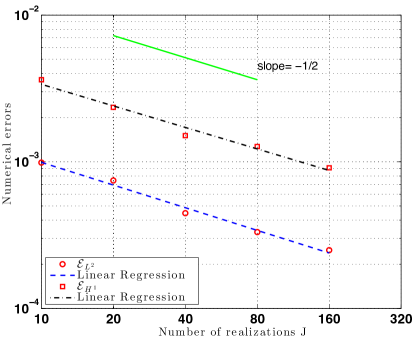
$J$	10	20	40	80	160
$\mathcal{E}_{L^{2}}$	9.8672e-04	7.4471e-04	4.4640e-04	3.3151e-04	2.4966e-04
$\mathcal{E}_{H^{1}}$	3.6240e-03	2.3475e-03	1.5080e-03	1.2696e-03	9.0903e-04

Next, we analyze some stochastic information of the system including the expectation of $u$ at the final time and a quantity of interest. In particular, we are mainly interested in comparing the ensemble simulation outputs with those from the individual simulations when the same set of samples is used. More precisely, we approximate the expected value $E[u(\omega,{\bf x},T)]$ by the EMC approximation

$$\Psi_{h}^{E}({\bf x})\coloneqq\frac{1}{J}\sum_{j=1}^{J}u_{h}^{E}(\omega_{j},{\bf x},T),$$

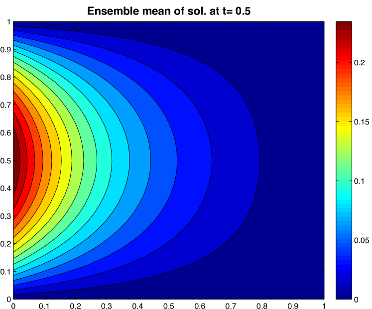
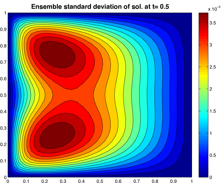
where $u_{h}^{E}(\omega_{j},{\bf x},T)$ is the $j$-th member solution in the ensemble-based simulation at time $T$. Taking the number of sample points to be $J=5000$, we compute the mean and standard deviation of the solutions at the final time, which are plotted in Figure 2 (left and middle).

Figure 2: Ensemble simulations: mean (left), standard deviation (middle) of solution at $t=0.5$, difference of the mean from that of the individual FEMC simulations (right).

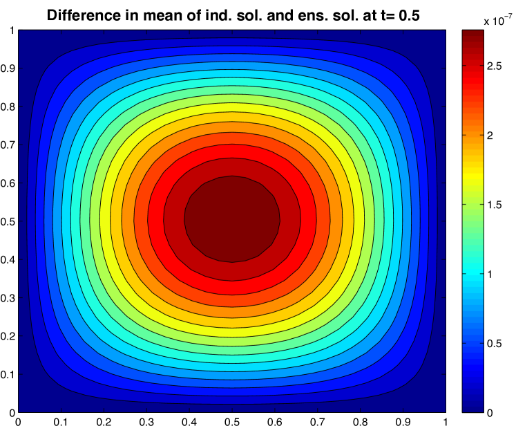
To quantify the performance of the EMC method, we compare the result with that of individual finite element Monte Carlo (FEMC) simulations using the same set of sample values. Denote the FEMC approximation solution by

$$\Psi_{h}^{I}({\bf x})\coloneqq\frac{1}{J}\sum_{j=1}^{J}u_{h}^{I}(\omega_{j},{\bf x},T),$$

where $u_{h}^{I}(\omega_{j},{\bf x},T)$ is the $j$-th independent solution at time $T$. The difference between $\Psi_{h}^{E}$ and $\Psi_{h}^{I}$ is shown in Figure 2 (right). It is observed that the difference is on the order of $10^{-7}$, which indicates the EMC method is able to provide the same accurate approximation as the individual FEMC simulations. However, the CPU time for the ensemble simulation is $1.4494\times 10^{4}$ seconds, while that of the individual simulations is $4.9197\times 10^{4}$ seconds. The former improves the computational efficiency by about 70%. Here, because the size of discrete system is small, we use Matlab and its LU matrix factorization for solving the linear system.

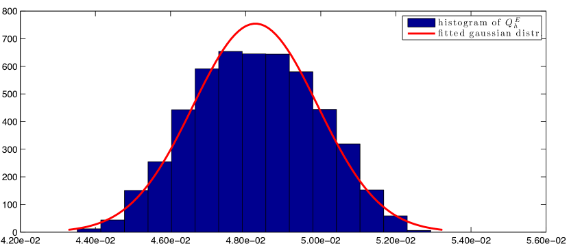
Following [19], we also calculate the quantity of interest

$$Q(\omega)=\int_{D}u(\omega,{\bf x},T)\,dD.$$

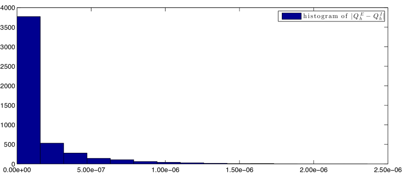
When the sample size is $J=5000$, the histogram of the quantity of interest obtained from the ensemble simulations, $Q_{h}^{E}$, is shown in Figure 3 (left) with a fitted gaussian distribution. We then do a comparison with the quantity of interest, $Q_{h}^{I}$, achieved from individual simulations at the same sampling set. The histogram of the differences in absolute value, $\left|Q_{h}^{E}-Q_{h}^{I}\right|$, is plotted in Figure 3 (right), which also illustrates that the EMC method outputs a close quantity of interest to the standard FEMC method.

Figure 3: Ensemble simulations: histogram of the quantity of interest $Q_{h}^{E}$ with a fitted gaussian distribution (left); histogram of the difference of the quantity in absolute value, $\left|Q_{h}^{E}-Q_{h}^{I}\right|$, between ensemble simulations and individual simulations (right).

6 Conclusion

We propose an ensemble-based algorithm in this paper to improve the computational efficiency for a group of numerical solutions to parabolic problems. The fundamental idea is to turn the linear systems associated to the group into a linear system with multiple right-hand-side vectors, which would reduce the computational time. We first analyze the ensemble scheme for deterministic equations, then develop the ensemble-based Monte Carlo method for stochastic equations. The effectiveness of both cases is demonstrated through rigorous error estimates and illustrated with numerical experiments. The approach can be easily extended to more general, nonlinear parabolic equations, which is one of the research directions we are pursuing.

References

- [1] I. Babuška, R. Tempone, and G. E. Zouraris, Solving elliptic boundary value problems with uncertain coefficients by the finite element method: the stochastic formulation, Computer methods in applied mechanics and engineering, 194 (2005), pp. 1251–1294.
- [2] S. Brenner and R. Scott, The mathematical theory of finite element methods, vol. 15, Springer Science & Business Media, New York, USA, 2007.
- [3] B. Ganapathysubramanian and N. Zabaras, Sparse grid collocation schemes for stochastic natural convection problems, Journal of Computational Physics, 225 (2007), pp. 652–685.
- [4] M. Gunzburger, N. Jiang, and M. Schneier, An ensemble-proper orthogonal decomposition method for the nonstationary navier–stokes equations, SIAM Journal on Numerical Analysis, 55 (2017), pp. 286–304.
- [5] M. Gunzburger, N. Jiang, and M. Schneier, A higher-order ensemble/proper orthogonal decomposition method for the nonstationary navier-stokes equations, (in press).
- [6] M. Gunzburger, N. Jiang, and Z. Wang, An efficient algorithm for simulating ensembles of parameterized flow problems, (submitted).
- [7] M. D. Gunzburger, C. G. Webster, and G. Zhang, Stochastic finite element methods for partial differential equations with random input data, Acta Numerica, 23 (2014), pp. 521–650.
- [8] J. C. Helton and F. J. Davis, Latin hypercube sampling and the propagation of uncertainty in analyses of complex systems, Reliability Engineering & System Safety, 81 (2003), pp. 23–69.
- [9] N. Jiang, A higher order ensemble simulation algorithm for fluid flows, Journal of Scientific Computing, 64 (2015), pp. 264–288.
- [10] N. Jiang, A second-order ensemble method based on a blended backward differentiation formula timestepping scheme for time-dependent navier–stokes equations, Numerical Methods for Partial Differential Equations, 33 (2017), pp. 34–61.
- [11] N. Jiang, S. Kaya, and W. Layton, Analysis of model variance for ensemble based turbulence modeling, Computational Methods in Applied Mathematics, 15 (2015), pp. 173–188.
- [12] N. Jiang and W. Layton, An algorithm for fast calculation of flow ensembles, International Journal for Uncertainty Quantification, 4 (2014).
- [13] N. Jiang and W. Layton, Numerical analysis of two ensemble eddy viscosity numerical regularizations of fluid motion, Numerical Methods for Partial Differential Equations, 31 (2015), pp. 630–651.
- [14] E. Kalnay, Atmospheric modeling, data assimilation and predictability, Cambridge University Press, New York, USA, 2003.
- [15] K. Liu and B. M. Rivière, Discontinuous galerkin methods for elliptic partial differential equations with random coefficients, International Journal of Computer Mathematics, 90 (2013), pp. 2477–2490.
- [16] L. Mathelin, M. Y. Hussaini, and T. A. Zang, Stochastic approaches to uncertainty quantification in CFD simulations, Numerical Algorithms, 38 (2005), pp. 209–236.
- [17] M. Mohebujjaman and L. G. Rebholz, An efficient algorithm for computation of mhd flow ensembles, Computational Methods in Applied Mathematics, 17 (2017), pp. 121–137.
- [18] H. Niederreiter, Random number generation and quasi-Monte Carlo methods, SIAM, Philadelphia, PA, USA, 1992.
- [19] F. Nobile and R. Tempone, Analysis and implementation issues for the numerical approximation of parabolic equations with random coefficients, International journal for numerical methods in engineering, 80 (2009), pp. 979–1006.
- [20] M. L. Parks, K. M. Soodhalter, and D. B. Szyld, A block recycled gmres method with investigations into aspects of solver performance, arXiv preprint arXiv:1604.01713, (2016).
- [21] A. Takhirov, M. Neda, and J. Waters, Time relaxation algorithm for flow ensembles, Numerical Methods for Partial Differential Equations, 32 (2016), pp. 757–777.
- [22] D. Xiu and J. S. Hesthaven, High-order collocation methods for differential equations with random inputs, SIAM Journal on Scientific Computing, 27 (2005), pp. 1118–1139.
- [23] X. Zhu, E. M. Linebarger, and D. Xiu, Multi-fidelity stochastic collocation method for computation of statistical moments, Journal of Computational Physics, 341 (2017), pp. 386–396.