Turbulent density fluctuations and proton heating rate in the solar wind from $9-20~{}R_{\odot}$

Abstract

We obtain scatter-broadened images of the Crab nebula at 80 MHz as it transits through the inner solar wind in June 2016 and 2017. These images are anisotropic, with the major axis oriented perpendicular to the radially outward coronal magnetic field. Using these data, we deduce that the density modulation index ($\delta N_{e}/N_{e}$) caused by turbulent density fluctuations in the solar wind ranges from 1.9 $\times 10^{-3}$ to 7.7 $\times 10^{-3}$ between 9 —- 20 $R_{\odot}$. We also find that the heating rate of solar wind protons at these distances ranges from $2.2\times 10^{-13}$ to $1.0\times 10^{-11}~{}\rm erg~{}cm^{-3}~{}s^{-1}$. On two occasions, the line of sight intercepted a coronal streamer. We find that the presence of the streamer approximately doubles the thickness of the scattering screen.

1 Introduction

The solar wind exhibits turbulent fluctuations in velocity, magnetic field, and density. Traditionally, researchers have attempted to understand this phenomenon within the framework of incompressible magnetohydrodynamic (MHD) turbulence (e.g., Goldstein et al. (1995)). However, density fluctuations are not explained in this framework, and remain a relative enigma despite noteworthy progress (e.g., Hnat et al. (2005); Shaikh & Zank (2010); Banerjee & Galtier (2014)). While most of the data used for solar wind turbulence studies are from in-situ measurements made by near-Earth spacecraft, density fluctuations can often been inferred via remote sensing observations, typically at radio wavelengths. Examples include angular broadening of point-like radio sources observed through the solar wind (Machin & Smith, 1952; Hewish & Wyndham, 1963; Erickson, 1964; Blesing & Dennison, 1972; Dennison & Blesing, 1972; Sastry & Subramanian, 1974; Armstrong et al., 1990; Anantharamaiah et al., 1994; Ramesh et al., 1999, 2001, 2012; Kathiravan et al., 2011; Mugundhan et al., 2016; Sasikumar Raja et al., 2016), interplanetary scintillations (IPS; Hewish et al. (1964); Cohen & Gundermann (1969); Ekers & Little (1971); Rickett (1990); Bisi et al. (2009); Manoharan et al. (2000); Tokumaru et al. (2012, 2016)), spacecraft beacon scintillations (Woo & Armstrong, 1979), interferometer phase scintillations using Very Long Baseline Interferometers (VLBI; Cronyn (1972)), spectral broadening using coherent spacecraft beacons (Woo & Armstrong, 1979) and radar echoes (Harmon & Coles, 1983).

A related problem is the issue of turbulent heating in the inner solar wind. It is well known that the expansion of the solar wind leads to adiabatic cooling, which is offset by some sort of heating process (Richardson et al., 1995; Matthaeus et al., 1999). The candidates for such extended heating range from resonant wave heating (Cranmer, 2000; Hollweg & Isenberg, 2002) to reconnection events (e.g., Cargill & Klimchuk (2004)). Some studies have attempted to link observations of density turbulence with kinetic Alfven waves that get resonantly damped on protons, consequently heating them (Ingale, 2015b; Chandran et al., 2009).

In this paper, we investigate the characteristics of turbulent density fluctuations and associated solar wind heating rate from $9-20~{}R_{\odot}$ using the anisotropic angular broadening of radio observations of the Crab nebula from June 9 to 22 in 2016 and 2017. The Crab nebula passes close to the Sun on these days every year. Since its radiation passes through the foreground solar wind, these observations give us an opportunity to explore the manner in which its angular extent is broadened due to scattering off turbulent density fluctuations in the solar wind. Anisotropic scatter-broadening of background sources observed through the solar wind has hitherto been reported only for small elongations ($\approx 2-6~{}R_{\odot}$) e.g., (Anantharamaiah et al., 1994; Armstrong et al., 1990). Imaging observations of the Crab nebula (e.g., Blesing & Dennison (1972); Dennison & Blesing (1972)) offer us an opportunity to investigate this phenomenon for elongations $\gtrsim 10R_{\odot}$. On 17 June 2016, 17 and 18 June 2017, a coronal streamer was present along the line of sight to the Crab nebula; this gives us an additional opportunity to study streamer characteristics. The Parker Solar Probe (Fox et al., 2016) is expected to sample the solar wind as close as 10 $R_{\odot}$. In-situ measurements from the SWEAP instrument aboard the PSP can validate our findings regarding the density turbulence level and the proton heating rate.

The rest of the paper is organized as follows: in § 2, we describe imaging observations of the Crab nebula made at Gauribidanur in June 2016 and 2017. The next section (§ 3) explains the methodology for obtaining the turbulence levels from these images. This includes a brief discussion of the structure function, some discussion of the inner scale of the density fluctuations, followed by the prescription we follow in computing the density fluctuations and solar wind heating rate at the inner scale. § 4 summarizes our main results and conclusions.

2 Observations: scatter-broadened images of the Crab nebula

The radio data were obtained with the Gauribidanur RAdioheliograPH (GRAPH; Ramesh et al. (1998); Ramesh (2011)) at 80 MHz during the local meridian transit of the Crab nebula. The GRAPH is a T-shaped interferometer array with baselines ranging from $\approx 80$ to $\approx 2600$ meters. The angular resolution is $\approx$ 5 arcmin at 80 MHz, and the minimum detectable flux ($5\sigma$ level) is $\approx 50$ Jy for 1 sec integration time and 1 MHz bandwidth. Cygnus A was used to calibrate the observations. Its flux density is $\approx 16296$ Jy at 80 MHz. The flux density of Crab nebula (when it is far from the Sun and is not therefore scatter-broadened by solar coronal turbulence) is $\approx 2015$ Jy at 80 MHz. We imaged the Crab nebula at different projected heliocentric distances shown in column (3) of Table-1 in the years 2016 and 2017.

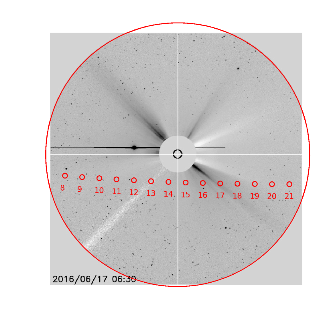
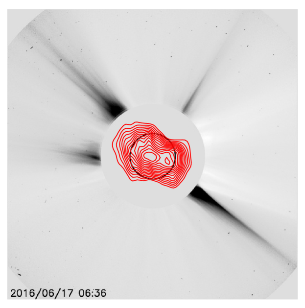
Figure 1: (left) SOHO/LASCO C3 image of the solar corona (inverted grey scale image) observed on 17 June 2016 at 06:30 UT is shown. The innermost black circle indicates the solar disk (radius $=1~{}R_{\odot}$). The next concentric circle is the occulting disk of the coronagraph and its radius is $3.5~{}R_{\odot}$. The outermost circle marks a heliocentric distance of $30~{}R_{\odot}$. In both the images, the black features are coronal streamers. Solar north is up and east is to the left. The small circles superposed on the image represent the location of the Crab nebula on different days during the period 8 June 2016 to 21 June 2016. Its closest approach to the Sun is on 14 June 2016 at a heliocentric distance of $\approx 5~{}R_{\odot}$. The coronal streamer in the south-west quadrant occults the Crab nebula on 17 June 2016 at a projected heliocentric distance $\approx 10.2~{}R_{\odot}$. The position angle (PA, measured counterclockwise from north) of the streamer is $\approx 235^{\circ}$. (right) SOHO/LASCO C2 image of the solar corona (inverted grey scale) on 17 June 2016 at 06:36 UT is shown. The red contours represent observations of the solar corona using the GRAPH at 80 MHz. The elongated radio contours correspond to emission from the streamers in north-east and south-west quadrants.

We have used white light images of the solar corona obtained with the Large Angle and Spectrometric Coronagraph (LASCO) onboard the SOlar and Heliospheric Observatory (SOHO) (Brueckner et al., 1995) for general context, and to identify features like coronal streamers. Figure 1 shows the white light images of the solar corona obtained with the LASCO C3 (left) and C2 (right) coronagraphs on 17 June 2016. The black features in both inverted grey scale images are coronal streamers. The location of the Crab nebula between 8 and 21 June 2016 is marked by the red circles on the LASCO C3 images. On 17 June 2016, the Crab nebula was observed through a streamer in the south-west quadrant. The streamer was associated with an active region NOAA 12555 located at heliographic coordinates S09W71. The contours superposed over the LASCO C2 image are from the GRAPH observations at 80 MHz showing radio emission from the streamers in north-east and south-west quadrants (Ramesh, 2000).

Some representative 80 MHz GRAPH images of the Crab nebula are shown in Figure 2. The image on 12 June 2016 was observed through the solar wind at $10.18~{}R_{\odot}$ during ingress. The one on 17 June 2016 was observed at $10.20~{}R_{\odot}$, while the one on 17 June 2017 at $9.41~{}R_{\odot}$ and the one on 18 June 2017 at $12.61~{}R_{\odot}$ during egress. The Crab nebula was occulted by a coronal streamer on 17 June 2016 and on 17 and 18 June 2017. These scatter-broadened images are markedly anisotropic. This aspect has been noted earlier, for the Crab nebula (Blesing & Dennison, 1972; Dennison & Blesing, 1972) as well as other sources (Anantharamaiah et al., 1994; Armstrong et al., 1990). Note that the major axis of these images is always perpendicular to the heliocentric radial direction (which is typically assumed to be the magnetic field direction at these distances) - this is especially evident when the Crab is occulted by a streamer. The parameters for all observations of the Crab nebula in 2016 and 2017 are tabulated in Table 1.

Figure 2: The image on 12 June 2016 shows the scatter broadened Crab nebula at a projected heliocentric distance of $10.18~{}R_{\odot}$ during its ingress into the inner solar wind. The images on 17 June 2016 (at $10.2~{}R_{\odot}$), 17 ($9.41~{}R_{\odot}$) and 18 June 2017 ($12.61~{}R_{\odot}$) depict the scatter broadened Crab nebula observed through coronal streamers during its egress from the solar wind. The arrows depict the sunward direction on each day. The major axis of each image is perpendicular to the magnetic field lines, which are directed radially outward from the Sun.

Figure 3 shows the observed peak flux density of the Crab nebula with respect to its projected heliocentric distance. The red circles and blue squares are for the 2016 and 2017 observations respectively. Note that, in a given year the data points obtained during ingress and egress were plotted together with the (projected) heliocentric distance.

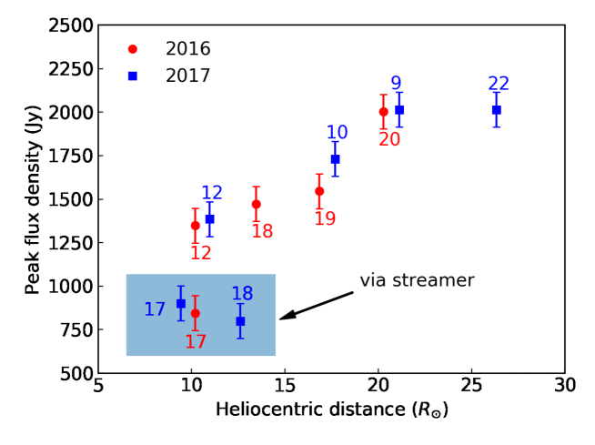
Figure 3: Peak flux density of the Crab nebula on different days of June 2016 (red circles) and 2017 (blue squares). The red and blue data points shown in the shaded area indicate instances when the Crab nebula was observed through a streamer in 2016 and 2017 respectively.

The observations shown in the shaded region in Figure 3 represent instances where the Crab nebula was occulted by a coronal streamer. Evidently, the peak flux density in these instances in considerably lower (as compared to the flux corresponding to a similar heliocentric distance, when the Crab is not occulted by a streamer). This could be because the line of sight to the Crab nebula passes through more coronal plasma during instances of streamer occultation, leading to enhanced scatter broadening. In turn, this leads to a larger scatter-broadened image and a consequent reduction in the peak flux density.

3 Turbulent density fluctuations and solar wind proton heating rate

The angular broadening observations of the Crab nebula described in the previous section can be used to infer the amplitude of turbulent density fluctuations and associated heating rate of protons in the solar wind. The main quantity inferred from the observations is the structure function, which is essentially the spatial Fourier transform of the visibility observed with a given baseline. The structure function is used to estimate $C_{N}^{2}$, the so-called “amplitude” of the turbulent density spectrum. The density spectrum is modelled as a power law with an exponential cutoff at an “inner scale”. We assume that the inner scale is given by the proton inertial length. We elaborate on these aspects in the subsections below.

3.1 Background electron density and the inner scale

Since our aim is to estimate the level of turbulent density fluctuations in relation to the background density ($N_{e}$), we use Leblanc density model (Leblanc et al., 1998) to estimate the $N_{e}$ in the solar wind,

$$N_{e}(R)=7.2~{}R^{-2}+1.95\times 10^{-3}~{}R^{-4}+8.1\times 10^{-7}~{}R^{-6}\,\,\,\,{\rm cm}^{-3}.$$ (1)

where ‘R’ is the heliocentric distance in units of astronomical units (AU, 1 AU = $215R_{\odot}$). The background electron density is used to compute the inner scale of the turbulent density spectrum. We assume that the inner scale $l_{i}$ is given by the proton inertial length (Verma et al., 1996; Leamon et al., 1999, 2000; Smith et al., 2001; Chen et al., 2014; Bruno & Trenchi, 2014), which is related to the background electron density by

$$l_{i}(R)=v_{A}(R)/\Omega_{p}(R)=2\pi/k_{i}(R)=228\times\sqrt{N_{e}(R)}\,\,\,{\rm km},$$ (2)

where $N_{e}$ is the electron density in ${\rm cm}^{-3}$, $k_{i}$ is the wavenumber, $v_{A}$ is the $\rm Alfv\acute{e}n$ speed and $\Omega_{i}$ is the proton gyrofrequency. We note that our definition differs slightly from that of Coles & Harmon (1989); Harmon (1989); Yamauchi et al. (1998) who use $l_{i}=3\times v_{A}(R)/\Omega_{p}(R)$ and $k_{i}=3/l_{i}$.

3.2 The structure function $D_{\phi}$

The structure function $D_{\phi}(s)$ is defined by (Prokhorov et al., 1975; Ishimaru, 1978; Coles & Harmon, 1989; Armstrong et al., 1990),

$$D_{\phi}(s)=-2ln\Gamma(s)=-2ln\left[V(s)/V(0)\right]\,,$$ (3)

where the quantity $s$ represents the baseline length, $\Gamma(s)$ is the mutual coherence function, $V(s)$ denotes the visibility obtained with a baseline of length $s$ and $V(0)$ denotes the “zero-length” baseline visibility. The quantity $V(0)$ is the peak flux density when the Crab nebula is situated far away from the Sun, and is unresolved; we set it to be $\approx 2015$ Jy at 80 MHz (Braude et al., 1970; McLean & Labrum, 1985). The images of the Crab nebula in Figure 2 are obtained by combining the visibilities from all the baselines available in the GRAPH. We are interested in the turbulent density fluctuations at the inner scale, which is the scale at which the turbulent spectrum transitions from a power law to an exponential turnover. This is typically the smallest measurable scale; we therefore compute the structure function corresponding to the longest available baseline (s = 2.6 km), since that corresponds to the smallest scale.

3.3 The amplitude of density turbulence spectrum ($C_{N}^{2}$)

The turbulent density inhomogeneities are represented by a spatial power spectrum, comprising a power law together with an exponential turnover at the inner scale:

$$P_{\delta n}(k,R)=C_{N}^{2}(R)(\rho^{2}~{}k_{x}^{2}+k_{y}^{2})^{-\alpha/2}\times\exp\biggl{[}-(\rho^{2}~{}k_{x}^{2}+k_{y}^{2})\bigg{(}{l_{i}(R)\over 2\pi}\bigg{)}^{2}\biggr{]}\,,$$ (4)

where $k=\sqrt{\rho~{}k_{x}^{2}+k_{y}^{2}}$ is the wavenumber, $k_{x}$ and $k_{y}$ are the wavenumber along and perpendicular to the large-scale magnetic field respectively. The quantity $\rho$ is a measure of the anisotropy of the turbulent eddies. In our calculations, we use the axial ratio of the scatter broadened images at 80 MHz (shown in Table 1) for $\rho$. The quantity $C_{N}^{2}$ is the amplitude of density turbulence, and has dimensions of ${\rm cm}^{-\alpha-3}$, where $\alpha$ is the power law index of the density turbulent spectrum. At large scales the density spectrum follows the Kolmogorov scaling law with $\alpha=11/3$. At small scales, (close to the inner scale, when $s\approx l_{i}$) the spectrum flattens to $\alpha=3$ (Coles & Harmon, 1989). Since we are interested in the density fluctuations near the inner scale, we use $\alpha=3$.

Many authors use analytical expressions for the structure function that are applicable in the asymptotic limits $s\ll l_{i}$ or $s\gg l_{i}$ (Coles et al., 1987; Armstrong et al., 2000; Bastian, 1994; Subramanian & Cairns, 2011). However, these expressions are not valid for situations (such as the one we are dealing with in this paper) where the baseline is comparable to the inner scale; i.e., $s\approx l_{i}$. We therefore choose to use the General Structure Function (GSF) which is valid in the $s\ll l_{i}$ and $s\gg l_{i}$ regimes as well as when $s\approx l_{i}$ (Ingale et al., 2015a). In the present case, largest baseline length $\approx 2.6$ km is comparable to the inner scale lengths $\approx 4.56$ km. The GSF is given by the following expression:

$${D_{\phi}(s)}=\frac{8\pi^{2}r_{e}^{2}\lambda^{2}\Delta L}{\rho~{}2^{\alpha-2}(\alpha-2)}{\Gamma\bigg{(}1-{{\alpha-2}\over 2}\bigg{)}}{{C_{N}^{2}(R)l_{i}^{\alpha-2}(R)}\over{(1-f_{p}^{2}(R)/f^{2})}}$$

$${\times\bigg{\{}{{}_{1}F_{1}}{\bigg{[}-{{\alpha-2}\over 2},~{}1,~{}-\bigg{(}{s\over l_{i}(R)}\bigg{)}^{2}\bigg{]}}-1\bigg{\}}}\,\,\,\,{\rm rad}^{2},$$ (5)

where ${{}_{1}F_{1}}$ is the confluent hyper-geometric function, $r_{e}$ is the classical electron radius, $\lambda$ is the observing wavelength, $R$ is the heliocentric distance (in units of $R_{\odot}$), $\Delta L$ is the thickness of the scattering medium, $f_{p}$ and f are the plasma and observing frequencies respectively. Substituting the model densities and $\alpha=3$ in Equation 3.3 enables us to calculate $C_{N}^{2}$. Following Sasikumar Raja et al. (2016), we assume the thickness of the scattering screen to be $\Delta L=(\pi/2)R_{0}$, where, $R_{0}$ is the impact parameter related to the projected heliocentric distance of the Crab nebula in units of cm. When the Crab nebula is occulted by a streamer, however, this estimate of $\Delta L$ is not valid. It is well known that the streamer owes its appearance to the fact that the line of sight to the streamer intercepts excess coronal plasma that is contained around the current sheet “fold”. It therefore stands to reason that the $\Delta L$ along a line of sight that intercepts a streamer will be larger than that along a line of sight that does not include a streamer. In view of this, we use the formula $\Delta L=(\pi/2)R_{0}$ and compute the density fluctuation amplitude and turbulent heating rate only for the instances where the Crab nebula is not occulted by a streamer.

In the instances where it is occulted by a streamer, we can estimate the extra line of sight path length implied by the presence of the streamer. In order to do this, we first compute the structure function (Eq 3.3) in the instances when the line of sight to the Crab nebula contains a streamer. We then estimate the ratio of this quantity to the structure function (at a similar heliocentric distance) when the line of sight does not intercept a streamer turns out to be $\approx 2$. For instance, $D_{\phi}(s=2.6\,{\rm km},\,\,{\rm June}\,17\,2016)/D_{\phi}(s=2.6\,{\rm km},\,\,{\rm June}\,12\,2016)=2.16$. On June 12 2016, the Crab nebula was situated at $10.18R_{\odot}$ and the line of sight to it did not pass through a streamer. On June 17 2016, the Crab nebula was situated at a similar projected heliocentric distance ($10.2R_{\odot}$), but the line of sight to it passed through a coronal streamer. From Eq (3.3), it is evident that this ratio is equal to the ratio of the $\Delta L$s in the two instances. In other words, the presence of a streamer approximately doubles the path length along the line of sight over which scattering takes place.

Although we show 80 MHz observations in this paper, we also have simultaneous observations at 53 MHz. The structure function (equation 3.3) is proportional to the square of the observing frequency (i.e., $D_{\phi}(s)~{}\propto~{}\lambda^{2}$). This predicts that the ratio of the structure functions at 80 and 53.3 MHz should be 0.44. Our observations yield a value of 0.43 for this ratio, and are thus consistent with the expected scaling.

3.4 Estimating the density modulation index ($\epsilon_{N_{e}}=\delta N_{k_{i}}/N_{e}$)

The density fluctuations $\delta N_{k_{i}}$ at the inner scale can be related to the spatial power spectrum (Equation 4) using the following prescription (Chandran et al., 2009)

$${\delta}N_{k_{i}}^{2}(R)\sim 4\pi k_{i}^{3}P_{\delta N}(R,k_{i})=4\pi C_{N}^{2}(R)k_{i}^{3-\alpha}e^{-1}\,,$$ (6)

where $k_{i}\equiv 2\pi/l_{i}$. We estimate ${\delta}N_{k_{i}}$ by substituting $C_{N}^{2}$ calculated in § 3.3 and using $\alpha=3$ in Equation 6. We then use this ${\delta}N_{k_{i}}$ and the background electron density ($N_{e}$, § 3.1) to estimate the density modulation index ($\epsilon_{N_{e}}$) defined by

$$\epsilon_{N_{e}}(R)\equiv{~{}\delta N_{k_{i}}(R)\over N_{e}(R)}\,$$ (7)

The density modulation index in the solar wind at different heliocentric distances is computed using Eq 7. The results are listed in column (6) of table 1. The numbers in table 1 show that the density modulation index ($\epsilon_{N_{e}}$) in the solar wind ranges from 1.9 $\times 10^{-3}$ to 7.7 $\times 10^{-3}$ in the heliocentric range $\approx 10-20~{}R_{\odot}$. We have carried out these calculations only for the instances where the Crab nebula is not occulted by a streamer.

3.5 Solar wind heating rate

We next use our estimates of the turbulent density fluctuations (${\delta}N_{k_{i}}$) to calculate the rate at which energy is deposited in solar wind protons, following the treatment of Ingale (2015b). The basic assumption used is that the density fluctuations at small scales are manifestations of low frequency, oblique ($k_{\perp}\gg k_{\parallel}$), $\rm Alfv\acute{e}n$ wave turbulence. The quantities $k_{\perp}$ and $k_{\parallel}$ refer to components of the wave vector perpendicular and parallel to the background large-scale magnetic field respectively. The turbulent $\rm Alfv\acute{e}n$ wave cascade transitions to such oblique $\rm Alfv\acute{e}n$ waves (often referred to as kinetic $\rm Alfv\acute{e}n$ waves) near the inner/dissipation scale. We envisage a situation where the turbulent $\rm Alfv\acute{e}n$ wave cascade resonantly damps on (and thereby heats) the protons at the inner scale. Since this implicitly assumes that the $\rm Alfv\acute{e}n$ waves do not couple to other modes at the inner scale, our estimate of the proton heating rate is an upper limit. As explained in § 3.1, we assume that the inner scale is the proton inertial length, which is expressible as $l_{i}=v_{\rm A}/\Omega_{p}$, where $v_{\rm A}$ is the $\rm Alfv\acute{e}n$ speed and $\Omega_{p}$ is the proton gyrofrequency. This way of writing the the proton inertial length emphasizes its relation to the resonant damping of $\rm Alfv\acute{e}n$ waves on protons.

The specific energy per unit time ($\epsilon\,,\,{\rm erg~{}cm^{-3}~{}s^{-1}}$) in the turbulent $\rm Alfv\acute{e}n$ wave cascade is transferred from large scales to smaller ones, until it dissipates at the inner/dissipation scale. The proton heating rate equals the turbulent energy cascade rate at the inner scale ($\epsilon_{k_{i}}$), which is given by (Hollweg, 1999; Chandran et al., 2009; Ingale, 2015b),

$$\epsilon_{k_{i}}(R)=c_{0}\rho_{p}k_{i}(R)\delta v_{k_{i}}^{3}(R)~{}\rm erg~{}cm^{-3}~{}s^{-1}\,,$$ (8)

where $c_{0}$ is a constant usually taken to be 0.25 (Howes et al., 2008; Chandran et al., 2009) and $\rho_{p}=m_{p}N_{e}(R)~{}\rm g~{}cm^{-3}$, with $m_{p}$ representing the proton mass in grams. The quantity $k_{i}=2\pi/l_{i}$ is the wavenumber corresponding to the inner scale (Eq 2) and $\delta v_{k_{i}}$ represents the magnitude of turbulent velocity fluctuations at the inner scale. The density modulation index $\epsilon_{N_{e}}$ and the turbulent velocity fluctuations are related via the kinetic $\rm Alfv\acute{e}n$ wave dispersion relation (Howes et al., 2008; Chandran et al., 2009; Ingale, 2015b)

$$\delta v_{k_{i}}(R)=\Bigg{(}{1+{\gamma_{i}k_{i}^{2}(R)\rho_{i}^{2}(R)}\over{k_{i}(R)l_{i}(R)}}\Bigg{)}\epsilon_{N_{e}}(R,k_{i})v_{A}(R)\,.$$ (9)

The adiabatic index $\gamma_{i}$ is taken to be 1 (Chandran et al., 2009) and the proton gyroradius ($\rho_{i}$) is given by

$$\rho_{i}(R)=102\times\mu^{1/2}T_{i}^{1/2}B^{-1}(R)~{}\rm cm,$$ (10)

where $\mu$ is the ion mass expressed in terms of proton mass ($\approx 1$) and $T_{i}$ is the proton temperature in eV. We use $T_{i}=86.22$ eV which corresponds to a temperature of $1\times 10^{6}$ K.

The $\rm Alfv\acute{e}n$ speed ($v_{A}$) in the solar wind is given by

$$v_{A}(R)=2.18\times 10^{11}\mu^{-1/2}N_{e}^{-1/2}(R)B(R)~{}\rm cm~{}s^{-1},$$ (11)

and the magnetic field stength (B) is taken to be the Parker spiral mangetic field in the ecliptic plane (Williams, 1995)

$$B(R)=3.4\times 10^{-5}R^{-2}(1+R^{2})^{1/2}~{}\rm Gauss,$$ (12)

where, ‘R’ is the heliocentric distance in units of AU. Equations (12), (11), (10), (9) and the density modulation index computed in § 3.4 are used in Eq (8) to compute the solar wind heating rate at different heliocentric distances. These values are tabulated in column (7) of Table 1. Figure 4 depicts the density modulation index and the solar wind heating rate graphically as a function of heliocentric distance.

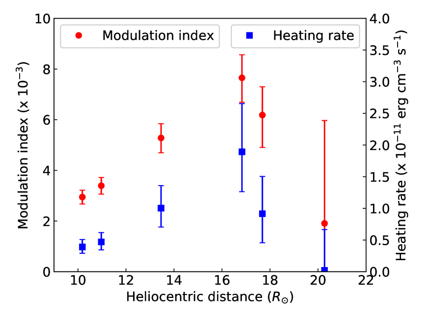
Figure 4: The variation of the density modulation index (red circles) and the solar wind proton heating rate (blue squares) with projected heliocentric distance. We note that the proton heating rate is correlated with the density modulation index.

S.No	Date	R	Peak flux density	$\rm\rho$	$\epsilon_{N_{e}}$	Heating rate
		$\rm(R_{\odot})$	(Jy)			($\rm erg~{}cm^{-3}~{}s^{-1}$)
(1)	(2)	(3)	(4)	(5)	(6)	(7)
Line of sight to the Crab does not include a streamer
1	12 June 2016	10.18	1349	1.48	2.9E-3	3.9E-12
2	18 June 2016	13.46	1473	1.76	5.3E-3	1.0E-11
3	19 June 2016	16.83	1546	1.69	7.7E-3	1.9E-11
4	20 June 2016	20.27	2003	1.98	1.9E-3	2.2E-13
5	09 June 2017	21.13	2015	1.48	-	-
6	10 June 2017	17.68	1732	1.57	6.2E-3	9.2E-12
7	12 June 2017	10.97	1386	1.50	3.4E-3	4.7E-12
8	22 June 2017	26.34	2015	1.40	-	-
Line of sight to the Crab includes a streamer
9	17 June 2016	10.20	845	2.44	-	-
10	17 June 2017	9.41	901	2.51	-	-
11	18 June 2017	12.61	800	1.65	-	-

Table 1: The table describes the observational quantities and the derived plasma parameters in the solar wind.

4 Summary and conclusions

4.1 Summary

We have imaged (figure 2) the Crab nebula at 80 MHz using the GRAPH in June 2016 and 2017, when it passed close to the Sun, and was obscured by the turbulent solar wind. Since the Crab nebula is a point source at 80 MHz when it is far from the Sun, these images are evidence of anisotropic scatter-broadening of radiation emanating from it as it passes through the turbulent solar wind. We calculate the structure function with the visibilities from the longest baselines (2.6 km) used in making these images. The structure function is used to infer the amplitude of the density turbulence spectrum ($C_{N}^{2}$), which is then used to compute the magnitude of the turbulent density fluctuations at the inner scale (Eq 6). This is then used to compute the density modulation index (Eq 7). Assuming that the turbulent $\rm Alfv\acute{e}n$ wave cascade in the solar wind dissipates on protons at the inner scale, we calculate the heating rate of protons in the solar wind (Eq 8). The density modulation index and solar wind proton heating rate are plotted in Figure 4 as a function of heliocentric distance.

4.2 Conclusions

The main conclusions of this paper pertain to the anisotropy of the scatter-broadened image of the Crab nebula, the density modulation index of the turbulent fluctuations in the solar wind and the solar wind proton heating rate from $9-20~{}R_{\odot}$. Some of the conclusions are:

• The 80 MHz scatter broadened images of the Crab nebula at heliocentric distances ranging from $9$ to $20~{}R_{\odot}$ in the solar wind are anisotropic, with axial ratios typically $\lesssim 2$ (table 1). The major axis of the Crab nebula is typically oriented perpendicular to the magnetic field direction, as in Anantharamaiah et al. (1994); Armstrong et al. (1990) (although their observations were at much smaller distances from the Sun).

• On 17 June 2016 and 17 June 2017, a coronal streamer was present along the line of sight to the Crab nebula. The line of sight to the Crab encountered more coronal plasma on these days, as compared to the days when a streamer was not present. The axial ratio of the scatter-broadened images on these days was somewhat larger ($\approx 2$, see table 1) and the peak flux density is considerably lower (figure 3), reflecting this fact. In the presence of a streamer, the path length over which scattering takes place was found to be approximately twice of that when the streamer was not present.

• The density modulation index ($\epsilon_{N_{e}}\equiv\delta N_{e}/N_{e}$) at the inner scale of the turbulent spectrum in the solar wind from $9-20~{}R_{\odot}$ ranges from 1.9 $\times 10^{-3}$ to 7.7 $\times 10^{-3}$ (see table 1). Earlier estimates of $\epsilon_{N_{e}}$ include Sasikumar Raja et al. (2016) who reported $0.001\lesssim\epsilon_{N_{e}}\lesssim 0.1$ from 10-45 $R_{\odot}$, $0.001\lesssim\epsilon_{N_{e}}\lesssim 0.02$ reported by Bisoi et al. (2014) in the distance range 56-—185 $R_{\odot}$ and $0.03\lesssim\epsilon_{N_{e}}\lesssim 0.08$ reported by Spangler & Spitler (2004) at 1 AU (215 $R_{\odot}$). The red circles in Figure 4 depict the modulation index as a function of heliocentric distance. Figure 4 shows that the modulation index in the heliocentric distance $12-18~{}R_{\odot}$ is relatively higher. As explained in Sasikumar Raja et al. (2016), this might be because the line of sight to the Crab nebula at these distances passes through the fast solar wind, which has relatively higher proton temperatures (Lopez & Freeman, 1986). Furthermore, the density modulation index is correlated with the proton temperature (Celnikier et al., 1987). Taken together, this implies that one could expect higher values for the density modulation index in the fast solar wind.

• We interpret the turbulent density fluctuations as manifestations of kinetic $\rm Alfv\acute{e}n$ wave turbulence at small scales. Assuming that the turbulent $\rm Alfv\acute{e}n$ wave cascade damps resonantly on the protons at the inner scale, we use our estimates of the density modulation index to calculate the proton heating rate in the solar wind. We find that the estimated proton heating rate in the solar wind from $9-20~{}R_{\odot}$ ranges from $2.2\times 10^{-13}$ to $1.0\times 10^{-11}~{}\rm erg~{}cm^{-3}~{}s^{-1}$ (blue squares in figure 4).

5 Acknowledgments

KSR acknowledges the financial support from the Science $\&$ Engineering Research Board (SERB), Department of Science $\&$ Technology, India (PDF/2015/000393). PS acknowledges support from the ISRO RESPOND program. AV is supported by NRL grant N00173-16-1-G029. We thank the staff of the Gauribidanur observatory for their help with the observations and maintenance of the antenna and receiver systems there. KSR acknowledges C. Kathiravan for the valuable discussions related to the GRAPH observations. SOHO/LASCO data used here are produced by a consortium of the Naval Research Laboratory (USA), Max-Planck-Institut fuer Aeronomie (Germany), Laboratoire d’Astronomie (France), and the University of Birmingham (UK). SOHO is a project of international cooperation between ESA and NASA. The authors would like to thank the anonymous referee for the valuable and constructive suggestions.

References

- Anantharamaiah et al. (1994) Anantharamaiah, K. R., Gothoskar, P., & Cornwell, T. J. 1994, J. Astrophys. Astron., 15, 387
- Armstrong et al. (2000) Armstrong, J. W., Coles, W. A., & Rickett, B. J. 2000, Journal of Geophysical Research (Space Physics), 105, 5149
- Armstrong et al. (1990) Armstrong, J. W., Coles, W. A., Rickett, B. J., & Kojima, M. 1990, The Astrophysical Journal, 358, 685
- Banerjee & Galtier (2014) Banerjee, S., & Galtier, S. 2014, Journal of Fluid Mechanics, 742, 230
- Bastian (1994) Bastian, T. S. 1994, The Astrophysical Journal, 426, 774
- Bisi et al. (2009) Bisi, M. M., Jackson, B. V., Buffington, A., et al. 2009, Solar Physics, 256, 201
- Bisoi et al. (2014) Bisoi, S. K., Janardhan, P., Ingale, M., et al. 2014, The Astrophysical Journal, 795, 69
- Blesing & Dennison (1972) Blesing, R. G., & Dennison, P. A. 1972, Proceedings of the Astronomical Society of Australia, 2, 84
- Braude et al. (1970) Braude, S. Y., Megn, A. V., Ryabov, B. P., & Zhouck, I. N. 1970, Ap&SS, 8, 275
- Brueckner et al. (1995) Brueckner, G. E., Howard, R. A., Koomen, M. J., et al. 1995, Sol. Phys., 162, 357
- Bruno & Trenchi (2014) Bruno, R., & Trenchi, L. 2014, The Astrophysical Journal, Letters, 787, L24
- Cargill & Klimchuk (2004) Cargill, P. J., & Klimchuk, J. A. 2004, ApJ, 605, 911
- Celnikier et al. (1987) Celnikier, L. M., Muschietti, L., & Goldman, M. V. 1987, A&A, 181, 138
- Chandran et al. (2009) Chandran, B. D. G., Quataert, E., Howes, G. G., Xia, Q., & Pongkitiwanichakul, P. 2009, The Astrophysical Journal, 707, 1668
- Chen et al. (2014) Chen, C. H. K., Leung, L., Boldyrev, S., Maruca, B. A., & Bale, S. D. 2014, Geophysical Research Letters, 41, 8081
- Cohen & Gundermann (1969) Cohen, M. H., & Gundermann, E. J. 1969, The Astrophysical Journal, 155, 645
- Coles & Harmon (1989) Coles, W. A., & Harmon, J. K. 1989, The Astrophysical Journal, 337, 1023
- Coles et al. (1987) Coles, W. A., Rickett, B. J., Codona, J. L., & Frehlich, R. G. 1987, The Astrophysical Journal, 315, 666
- Cranmer (2000) Cranmer, S. R. 2000, ApJ, 532, 1197
- Cronyn (1972) Cronyn, W. M. 1972, ApJ, 174, 181
- Dennison & Blesing (1972) Dennison, P. A., & Blesing, R. G. 1972, Proceedings of the Astronomical Society of Australia, 2, 86
- Ekers & Little (1971) Ekers, R. D., & Little, L. T. 1971, Astronomy & Astrophysics, 10, 310
- Erickson (1964) Erickson, W. C. 1964, ApJ, 139, 1290
- Fox et al. (2016) Fox, N. J., Velli, M. C., Bale, S. D., et al. 2016, Space Sci. Rev., 204, 7
- Goldstein et al. (1995) Goldstein, M. L., Roberts, D. A., & Matthaeus, W. H. 1995, ARA&A, 33, 283
- Harmon (1989) Harmon, J. K. 1989, Journal of Geophysical Research (Space Physics), 94, 15399
- Harmon & Coles (1983) Harmon, J. K., & Coles, W. A. 1983, ApJ, 270, 748
- Hewish et al. (1964) Hewish, A., Scott, P. F., & Wills, D. 1964, Nature, 203, 1214
- Hewish & Wyndham (1963) Hewish, A., & Wyndham, J. D. 1963, Monthly Notices of the Royal Astronomical Society, 126, 469
- Hnat et al. (2005) Hnat, B., Chapman, S. C., & Rowlands, G. 2005, Physical Review Letters, 94, 204502
- Hollweg (1999) Hollweg, J. V. 1999, J. Geophys. Res., 104, 14811
- Hollweg & Isenberg (2002) Hollweg, J. V., & Isenberg, P. A. 2002, Journal of Geophysical Research (Space Physics), 107, 1147
- Howes et al. (2008) Howes, G. G., Cowley, S. C., Dorland, W., et al. 2008, Journal of Geophysical Research (Space Physics), 113, A05103
- Ingale (2015b) Ingale, M. 2015b, ArXiv e-prints, arXiv:1509.07652
- Ingale et al. (2015a) Ingale, M., Subramanian, P., & Cairns, I. 2015a, Monthly Notices of the Royal Astronomical Society, 447, 3486
- Ishimaru (1978) Ishimaru, A. 1978, Wave propagation and scattering in random media, Vol.1 (New York: Academic Press)
- Kathiravan et al. (2011) Kathiravan, C., Ramesh, R., Barve, I. V., & Rajalingam, M. 2011, ApJ, 730, 91
- Leamon et al. (2000) Leamon, R. J., Matthaeus, W. H., Smith, C. W., et al. 2000, The Astrophysical Journal, 537, 1054
- Leamon et al. (1999) Leamon, R. J., Smith, C. W., Ness, N. F., & Wong, H. K. 1999, Journal of Geophysical Research (Space Physics), 104, 22331
- Leblanc et al. (1998) Leblanc, Y., Dulk, G. A., & Bougeret, J.-L. 1998, Sol. Phys., 183, 165
- Lopez & Freeman (1986) Lopez, R. E., & Freeman, J. W. 1986, Journal of Geophysical Research (Space Physics), 91, 1701
- Machin & Smith (1952) Machin, K. E., & Smith, F. G. 1952, Nature, 170, 319
- Manoharan et al. (2000) Manoharan, P. K., Kojima, M., Gopalswamy, N., Kondo, T., & Smith, Z. 2000, ApJ, 530, 1061
- Matthaeus et al. (1999) Matthaeus, W. H., Zank, G. P., Smith, C. W., & Oughton, S. 1999, Physical Review Letters, 82, 3444
- McLean & Labrum (1985) McLean, D. J., & Labrum, N. R. 1985, Solar radiophysics: Studies of emission from the sun at metre wavelengths
- Mugundhan et al. (2016) Mugundhan, V., Ramesh, R., Barve, I. V., et al. 2016, ApJ, 831, 154
- Prokhorov et al. (1975) Prokhorov, A. M., Bunkin, F. V., Gochelashvili, K. S., & Shishov, V. I. 1975, Proc. IEEE, 63, 790
- Ramesh (2000) Ramesh, R. 2000, Journal of Astrophysics and Astronomy, 21, 237
- Ramesh (2011) —. 2011, Bull. Astron. Soc. India Conf. Ser., 2, 55
- Ramesh et al. (2012) Ramesh, R., Kathiravan, C., Barve, I. V., & Rajalingam, M. 2012, ApJ, 744, 165
- Ramesh et al. (2001) Ramesh, R., Kathiravan, C., & Sastry, C. V. 2001, The Astrophysical Journal, 548, L229
- Ramesh et al. (1999) Ramesh, R., Subramanian, K. R., & Sastry, C. V. 1999, Sol. Phys., 185, 77
- Ramesh et al. (1998) Ramesh, R., Subramanian, K. R., SundaraRajan, M. S., & Sastry, C. V. 1998, Solar Physics, 181, 439
- Richardson et al. (1995) Richardson, J. D., Paularena, K. I., Lazarus, A. J., & Belcher, J. W. 1995, Geophys. Res. Lett., 22, 325
- Rickett (1990) Rickett, B. J. 1990, Annual Review of Astronomy & Astrophysics, 28, 561
- Sasikumar Raja et al. (2016) Sasikumar Raja, K., Ingale, M., Ramesh, R., et al. 2016, Journal of Geophysical Research (Space Physics), 121, 11605
- Sastry & Subramanian (1974) Sastry, C. V., & Subramanian, K. R. 1974, Indian Journal of Radio and Space Physics, 3, 196
- Shaikh & Zank (2010) Shaikh, D., & Zank, G. P. 2010, MNRAS, 402, 362
- Smith et al. (2001) Smith, C. W., Mullan, D. J., Ness, N. F., Skoug, R. M., & Steinberg, J. 2001, Journal of Geophysical Research (Space Physics), 106, 18625
- Spangler & Spitler (2004) Spangler, S. R., & Spitler, L. G. 2004, Physics of Plasmas, 11, 1969
- Subramanian & Cairns (2011) Subramanian, P., & Cairns, I. 2011, Journal of Geophysical Research (Space Physics), 116, A03104
- Tokumaru et al. (2016) Tokumaru, M., Fujiki, K., Kojima, M., et al. 2016, AIP Conference Proceedings, 1720, doi:http://dx.doi.org/10.1063/1.4943827
- Tokumaru et al. (2012) Tokumaru, M., Kojima, M., & Fujiki, K. 2012, Journal of Geophysical Research (Space Physics), 117, A06108
- Verma et al. (1996) Verma, M. K., Roberts, D. A., Goldstein, M. L., Ghosh, S., & Stribling, W. T. 1996, Journal of Geophysical Research (Space Physics), 101, 21619
- Williams (1995) Williams, L. L. 1995, The Astrophysical Journal, 453, 953
- Woo & Armstrong (1979) Woo, R., & Armstrong, J. W. 1979, Journal of Geophysical Research (Space Physics), 84, 7288
- Yamauchi et al. (1998) Yamauchi, Y., Tokumaru, M., Kojima, M., Manoharan, P. K., & Esser, R. 1998, Journal of Geophysical Research (Space Physics), 103, 6571