A \DeclareBoldMathCommand\cBB \DeclareBoldMathCommand\cQQ \DeclareBoldMathCommand\cCC \DeclareBoldMathCommand\cII
Solving nonlinear circuits with pulsed excitation by multirate partial differential equations
Abstract
In this paper the concept of Multirate Partial Differential Equations (MPDEs) is applied to obtain an efficient solution for nonlinear low-frequency electrical circuits with pulsed excitation. The MPDEs are solved by a Galerkin approach and a conventional time discretization. Nonlinearities are efficiently accounted for by neglecting the high-frequency components (ripples) of the state variables and using only their envelope for the evaluation. It is shown that the impact of this approximation on the solution becomes increasingly negligible for rising frequency and leads to significant performance gains.
Index Terms:
Finite element analysis, Nonlinear circuits, Numerical simulation, Multirate partial differential equations.I Introduction
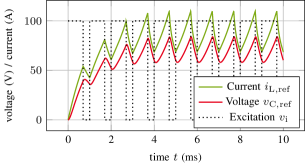
Multiscale and multirate problems occur naturally in many applications from electrical engineering. Classical discretization schemes are often inefficient in these cases and it is preferable to address the dynamics of each scale separately. In time domain the multirate phenomenon is often characterized by the fact that some solution components are active while the majority is latent (e.g. behind a low-pass filter [1]) or by problems with oscillatory solutions that are composed of multiple frequencies. An example is depicted in Fig. 1, it consists of a fast periodically varying ripple and a slowly varying envelope.
Multirate Partial Differential Equations (MPDEs) have been successfully applied in nonlinear high-frequency applications with largely separated time scales [2, 3]. Various methods have been proposed for the numerical solution of the MPDEs, e.g. harmonic balance [2], shooting methods, classical time stepping [4] or a combination of both [5]. Instead of the Fourier basis functions, one can also use classical nodal basis functions or more sophisticated problem-specific basis functions as for example the pulse width modulation (PWM) basis functions [6, 7].
This contribution focuses on improving the efficiency of the numerical solution of nonlinear MPDEs with a high-frequent pulsed excitation. In contrast to prior works, we propose neglecting the influence of high-frequency components on the nonlinearity. Consequently, the nonlinear relation is evaluated using only the envelope of the state variables.
The paper is structured as follows: after this introduction, Section II presents the multirate formulation. Section III discusses the Galerkin approach in time domain and the extraction of the envelope to evaluate nonlinear behavior. Section IV gathers numerical results based on the buck converter benchmark example and discusses the accuracy and efficiency of the modified method. Finally, conclusions are drawn.
II Multirate formulation
Spatial discretization of low-frequency field formulations as, e.g. electro- or magneto-quasi-statics [8], or network models of power converter circuits as, e.g. the buck converter in Fig. 2 lead to (nonlinear) systems of ordinary or differential algebraic equations of the form
| (1) |
with an initial condition , where is the vector of state variables, are matrices that may depend on the solution and is the excitation vector.
The system of equations (1) is hereafter rewritten as MPDEs [2, 3, 7] in terms of the two time scales and
| (2) |
where and are the multivariate forms of and . If fulfills the relation , the solution of the original problem can be extracted from the solution of the MPDEs by [2].
Let denote the slow time scale and the fast time scale, which is furthermore assumed to be periodic. Without limiting the generality of the approach, we choose such that the right-hand-side only depends on the fast time scale [7].

III Numerical method
System (2) can be numerically solved either using a Galerkin framework, shooting methods, classical time stepping or a combination. Here, we propose to use a variational setting, i.e. a Galerkin approach, for the fast time scale and a conventional time stepping for the slowly varying envelope.
III-A Galerkin in time domain
We represent the solution by an expansion of suitable basis functions and coefficients . The approximated state variables can be written as the series
| (3) |
with , where is the switching cycle of the excitation and mod denotes the modulo operation. Since we deal with pulsed right-hand-sides, we choose the PWM basis functions of [7], although constructed for linear problems [6]. The zero-th basis function is constant and the corresponding coefficient defines the envelope of the -th solution component. The first basis function is defined by
where is a free parameter, which can be chosen according to the duty cycle of the PWM, i.e. between 0 and 1. The basis functions of higher degree , are obtained recursively by integrating and orthonormalizing with respect to the scalar product, [6, 7].
Finally, a Galerkin approach is applied on the interval of one period, which yields
| (4) | ||||
for all . The integration with respect to leads to a system of differential (algebraic) equations in , which can be solved by conventional time integration.
III-B Treatment of nonlinearity
During time integration of (4), the integrals have to be evaluated every time step due to their nonlinear dependency on the solution. This may lead to an unnecessary increase of the computational effort as the ripple components are often small in comparison with the magnitude of the envelope. Consequently, one can save computational time by ignoring the ripple components of the solution and only using its envelope for the evaluation of the nonlinearity.
As mentioned before, the envelope is stored in the vector of coefficients given by
| (5) |
Let us abstractly define a function , which extracts the envelope from , i.e.
| (6) |
which is in the case of PWM basis functions the zero-th components, i.e.
| (7) |
Therefore the matrices , only depend on and the evaluation of (4) simplifies significantly. Equation (4) becomes
| (8) | ||||
for all , where the matrices and are independent of . Introducing
| (9) | ||||
| (10) |
in equation (8), we get
| (11) |
where the matrices are given by
| (12) | ||||
| (13) | ||||
| and denotes the Kronecker product. The right-hand-side vector is given by | ||||
| (17) | ||||
Eventually, system (11) can be more efficiently solved by conventional time discretization in the sense that larger time steps can be used than for the original problem (1). However, drawbacks are the approximation of the nonlinearity and the increased size of the matrices, i.e. , and , which is a similar tradeoff as in harmonic balance [2].
IV Numerical Results
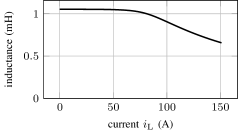
The numerical tests are performed on the simplified buck converter model [6] using a nonlinear coil, whose characteristic is shown in Fig. 4. The code is implemented in GNU Octave [9]; for time integration the high-order implicit Runge-Kutta method Radau5 from odepkg is used, [10, 11]. As basis functions we choose the problem-specific PWM basis functions introduced earlier.
The reference solution to which all results are compared is calculated directly by solving (1) with a very accurate time discretization (). The buck converter is operated in the range of frequencies from to . To determine the accuracy of the MPDE approach the relative -error of the buck converter voltage
| (18) |
with respect to is approximated by numerical quadrature. This calculation is performed for each frequency .
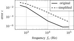
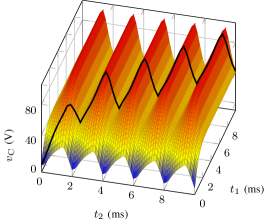
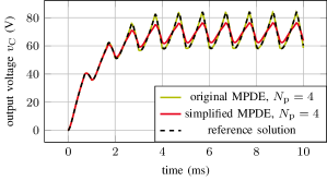
The MPDE solution is expanded using basis functions and (11) is solved using a tolerance of . The result is exemplary depicted in Fig. 3. Fig. 5 shows the error of the approach without (denoted as “original approach”) and with the simplified evaluation of the nonlinearity (8) (denoted as “simplified approach”) with respect to the frequency. Without the simplification, the integrals in (4) are evaluated using Gauss-Kronrod quadrature and lead to an accuracy of for frequencies kHz. As expected, the higher the frequency, the higher the accuracy of the method since the magnitude of the ripples in relation to the envelope decreases. The simplified approach introduces an additional error due to the approximation of the integrals. However, the accuracy for kHz, i.e., , is still sufficient for most applications. Fig. 7 shows the solutions of reference, simplified and original MPDE approach versus time at a low frequency Hz. Here, the error committed in the simplified approach is clearly distinguishable.
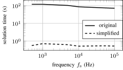
Table I shows the speedup (in terms of time for solving the equation systems) of the simplified MPDE approach compared to a conventional time discretization at the same accuracy. For higher frequency, the conventional time discretization of (1) becomes more and more inefficient as a higher number of ripples has to be resolved. The MPDE approach on the contrary resolves the ripples with the Galerkin approach so that the time discretization resolves only the envelope. This leads to a solution time almost independent of the frequency, i.e., approximately s for the simplified and s for the original approach, see Fig. 6. The higher solution time of the original approach is a result of the evaluation of the integrals in each time step. Thus the speedup of the original approach is much lower compared to the simplified approach.
V Conclusion
The MPDE approach is applied to a nonlinear low-frequency example with pulsed excitation. The solution is obtained by a Galerkin approach and time discretization. To evaluate the nonlinearity the ripple components due to the pulsed excitation are neglected and only the envelope is used. The accuracy of the proposed method rises with increasing excitation frequency and the method offers a considerable speedup compared to conventional time discretization with the same accuracy.
Acknowledgement
This work is supported by the ‘Excellence Initiative’ of German Federal and State Governments and the Graduate School CE at TU Darmstadt and in part by the Walloon Region of Belgium (WBGreen FEDO, grant RW-1217703).
| (kHz) | approx. speedup | approx. error |
|---|---|---|
| 10 | 60 | |
| 50 | 400 | |
| 100 | 1000 |
References
- [1] S. Schöps, H. De Gersem, and A. Bartel, “A cosimulation framework for multirate time-integration of field/circuit coupled problems,” IEEE Trans. Magn., vol. 46, no. 8, pp. 3233–3236, Jul. 2010.
- [2] H. G. Brachtendorf, G. Welsch, R. Laur, and A. Bunse-Gerstner, “Numerical steady state analysis of electronic circuits driven by multi-tone signals,” Electr. Eng., vol. 79, no. 2, pp. 103–112, 1996.
- [3] J. Roychowdhury, “Analyzing circuits with widely separated time scales using numerical PDE methods,” IEEE Trans. Circ. Syst. Fund. Theor. Appl., vol. 48, no. 5, pp. 578–594, May 2001.
- [4] T. Mei, J. Roychowdhury, T. Coffey, S. Hutchinson, and D. Day, “Robust, stable time-domain methods for solving MPDEs of fast/slow systems,” IEEE Trans. Comput. Aided. Des. Integrated Circ. Syst., vol. 24, no. 2, pp. 226–239, Feb. 2005.
- [5] K. Bittner and H. G. Brachtendorf, “Adaptive multi-rate wavelet method for circuit simulation,” Radioengineering, vol. 23, no. 1, Apr. 2014.
- [6] J. Gyselinck, C. Martis, and R. V. Sabariego, “Using dedicated time-domain basis functions for the simulation of pulse-width-modulation controlled devices – application to the steady-state regime of a buck converter,” in Electromotion 2013, Cluj-Napoca, Romania, Oct. 2013.
- [7] A. Pels, J. Gyselinck, R. V. Sabariego, and S. Schöps, “Multirate partial differential equations for the efficient simulation of low-frequency problems with pulsed excitations,” 2017, arXiv 1707.01947.
- [8] H. A. Haus and J. R. Melcher, Electromagnetic Fields and Energy. Prentice-Hall, 1989.
- [9] J. W. Eaton, D. Bateman, S. Hauberg, and R. Wehbring, The GNU Octave 4.0 Reference Manual 1/2: Free Your Numbers. Samurai Media Limited, Oct. 2015. [Online]. Available: http://www.gnu.org/software/octave/doc/interpreter
- [10] E. Hairer and G. Wanner, “Stiff differential equations solved by radau methods,” J. Comput. Appl. Math., vol. 111, no. 1–2, pp. 93–111, 1999.
- [11] T. Treichl and J. Corno, ODEpkg – A package for solving ordinary differential equations and more., 0th ed., GNU Octave, 2015. [Online]. Available: https://octave.sourceforge.io/odepkg/