Analysis of blood flow in one dimensional elastic artery using Navier-Stokes conservation laws

Student: Cristóbal Rodero Gómez^1,3

Tutors: J. Alberto Conejero²
    Ignacio García-Fernández³

¹Facultat de Matemàtiques, Universitat de València
²IUMPA, Universitat Politècnica de València
³CoMMLab, Departament d’Informàtica, Universitat de València

“Remember that all models are wrong; the practical question is how wrong do they have to be to not be useful.”

George Box, statistician.

“Applied math pattern: In principle you could just … but here’s why that won’t work in practice, and what you need to do instead.”

@AnalysisFact, tweet from Aug. 14th, 2017.

Abstract

In the last years, medical computer simulation has seen a great growth in several scientific branches, from modelling to numerical methods, going through computer science. The main goals of this incipient discipline are testing hypotheses before an intervention, or see what effect could have a drug in the system before actually taking it, among others.
In this work we deduce from the most basic physical principles a one dimensional model for the simulation of blood flow in elastic arteries. We will provide some historical background, as well as a brief state of the art of these models. We will also study from a calculus point of view the equations of the model obtained, achieving an original result for the formation of shock waves in compliant vessels. Afterwards we will make some numerical simulations using Galerkin Discontinuous Finite Element Method. Since this is actually a family of methods, we will motivate and detail the elections and the implementation strategies.

Contents

1. 1 Introduction and brief historical background
   1. 1.1 Historical review
   2. 1.2 Objectives and structure of the work
2. 2 One-dimensional blood flow modelling with non-rigid artery
   1. 2.1 Governing equations
      1. 2.1.1 Continuity equation
      2. 2.1.2 Momentum equation
      3. 2.1.3 The tube laws
3. 3 Theoretical analysis applied to the Navier-Stokes problem
   1. 3.1 Method of characteristics
      1. 3.1.1 Derivation of the method via calculus of variations
      2. 3.1.2 Setting of the Navier-Stokes system
      3. 3.1.3 Characteristic variables
   2. 3.2 Sufficient conditions for smooth flow
      1. 3.2.1 Shock wave formation in compliant arteries
4. 4 Discontinuous Galerkin Method
   1. 4.1 Notation
      1. 4.1.1 Measure and integral Lebesgue notation
   2. 4.2 DG space (semi)discretisation
      1. 4.2.1 Election of test and basis functions
      2. 4.2.2 Numerical flux
5. 5 Implementation and results
   1. 5.1 Spatial integration
   2. 5.2 Temporal integration
   3. 5.3 Test case
   4. 5.4 Convergence and stability
   5. 5.5 Biomedical simulations dependent on the parameters
6. 6 Conclusions and future work
7. A Biological parameters

List of Figures

1. 2.1 Artery as a compliant tube.
2. 2.2 Chronology of the models presented on the tube law subsection.
3. 3.1 Scheme of different types of characteristic curves.
4. (a) Characteristic curves with constant slope.
5. (b) (Forward) characteristic curves with variable slope.
6. (c) Formation of a shock wave.
7. 3.2 The subdomains $D_{1}$, $D_{2}$ and $D_{2}^{T}$.
8. 4.1 One dimensional finite element discretisation.
9. 4.2 Change of coordinates from global to local at an element.
10. 4.3 Condition number (in norm $1$) of the matrix $\mathcal{M}$. As we can see, it grows almost exponentially.
11. 4.4 Legendre’s polynomials up to degree $5$.
12. 4.5 Condition number (in norm $1$) of the matrix $\mathcal{M}$. As we can see, it grows linearly.
13. 5.1 Inflow velocity in the same units as the initial velocity.
14. 5.2 Advection of travelling waves at times $t=2.5$, $t=12.5$, $t=20$.
15. 5.3 Discontinuity measure varying $N_{\textrm{el}}$, $\Delta t$, $P$ and the time when it is measured.
16. 5.4 Maximum arterial amplitude (in centimetres) as a function of the BPM and $\beta$.
17. 5.5 Maximum blood flow velocity (in m/s) as a function of the BPM and $\beta$.

Chapter 1 Introduction and brief historical background

In the last years, medical computer simulation has seen a great growth in several scientific branches, from modelling to numerical methods, going through computer science. The main goals of this incipient discipline are testing hypotheses before an intervention, or see what effect could have a drug in the system before actually taking it, among others. In this chapter we will name some of the most important contributors to this discipline. We will focus on the physics’ (specially mechanics’) point of view, and for historical reasons, up to $20$^th century. In subsequent chapters the most recent computational scientific progress will be presented.

1.1 Historical review

For obvious reasons, one of the most important systems to be simulated is the cardiovascular system. Here, medicine works together with physics: electrophysiology (the nerve impulses that stimulates the heart), elasticity theory (in the movement of the heart, the arteries…) or fluid dynamics (the blood’s behaviour). The first models are often simplified versions of reality, neglecting some effects or reducing dimensionality. Taking this into account, the modelling of human arterial system can be traced back to Euler in $1775$, who submitted an essay as an entry in a prize competition set by the Academy of Sciences in Dijon [35]. He derived a one-dimensional simplification using partial differential equations, arriving to the equations of conservation of mass and momentum — they will be explained later — in a distensible tube. Euler posited some rather unrealistic constitutive laws (tube laws) for arteries and unsuccessfully tried to solve the equations. He tried to solve the problem as he had done for rigid tubes: by reducing them to a single equation that could be solved by integration. Quoting, “In motu igitur sanguinis explicando easdem offendimus insuperabiles difficultates[…]”, loosely translated as “On the explanation of the blood motion we stumble upon the same insuperable difficulties”. This letter was lost over a century, being discovered and published by the Euler Opera postuma project in $1862$.

Now, according to [85], the next major event in the history of quantitative haemodynamics is the lecture delivered to the Royal Society in $1808$ by Young [131]. In the lecture, he stated the correct formula for the wave speed in an artery but gave no derivation of it. In an associated paper, he does give a derivation based on an analogy to Newton’s derivation of the speed of sound in a compressible gas, altogether with some numerical guesses [130].

The development by Poiseuille ($1799$–-$1869$) of his law of flow in tubes is the next landmark in arterial mechanics. Because of its simplicity, this law has become the benchmark against which all other flows in tubes are compared, although in arteries is quite difficult to observe it. Despite its shortcomings, it is cited by many medical and physiological textbooks as the law that governs flow in the whole of vasculature. Poiseuille, who trained as a physician, conducted a very thorough investigation of flow in capillary tubes motivated by his studies of the mesenteric microcirculation of the frog. All his experiments and conclusions were finally approved for publication in $1846$ [91]. It seems that Stokes also derived Poiseuille’s law from the Navier-Stokes equation as early as $1845$ but did not publish the work because he was unsure about the validity of the no-slip condition at the tube walls [115].

The question of the speed of travel of waves in elastic tubes was studied theoretically and experimentally by Weber and Weber and published in 1866 [123, 124].

Riemann ($1826$–$1866$) did not work on arterial mechanics or waves in elastic tubes, but he did make an important contribution to the subject when he published a general solution for hyperbolic systems of partial differential equations in $1853$ [99]. Briefly, his work provides a general solution for a whole class of linear and nonlinear partial differential equations by observing that along directions defined by the eigenvalues of the matrix of coefficients of the differential terms, the partial differential equations reduce to ordinary differential equations. This method (the method of characteristics) will be explained in a more detailed way in subsequent chapters. The first application of the theory to arterial flows is probably the work of Lambert, who applied the theory to arteries using experimental measurements of the radius of the artery as a function of pressure [67]. The approach was developed by Skalak [107] and most completely by Anliker and his colleagues who mounted a systematic study of the different elements of the vascular system with the goal of synthesising a complete description of the arterial system using the method of characteristics [3, 53] [113, 114].

In $1877$–$1878$, two more important works on the wave speed in elastic tubes were published. Moens ($1846$–$1891$) [81] published a very careful experimental paper on wave speed in arteries and Korteweg ($1848$–$1941$) [62] published a theoretical study of the wave speed. Korteweg’s analysis showed that the wave speed was determined both by the elasticity of the tube wall and the compressibility of the fluid.

Frank ($1865$–$1944$) was another important contributor in quantitative physiology. One of his major contributions is a series of three papers. In [43], he introduces the theory of waves in arteries. In [45], he correctly derives the wave speed in terms of the elasticity. Finally, in [44], he considers the effect of viscosity, the motion of the wall and the energy of the pulse wave before turning to a number of examples of special cases. These examples include the use of Fourier analysis and probably the first treatment of the reflections of the pulse wave, including the reflection and transmission coefficients due to a bifurcation.

Many clinical cardiologists in the early twentieth century contributed to our understanding of the form and function of the cardiovascular system, but relatively few contributed significantly to our understanding of arterial mechanics (see [85] and the references therein).

1.2 Objectives and structure of the work

Now that a brief historical background has been introduced we notice that we are dealing with a non trivial and relevant problem. The main aim of this work is, therefor, to achieve an efficient simulation of blood flow in compliant arteries. In order to do that, the physical model will be presented for a further mathematical analysis. Once the main features of this analysis have been extracted, via an appropriate numerical method, some simulations will be performed. A review of some of the most important models, both numerical and theoretical has been made along the work.

Hence, this document is structured as follow. In chapter 2 we present the main equations for the modelling of arterial flow. We will present the widely accepted conservation equations in section 2.1. In the same section, the main problem of no scientific agreement will be presented, along with a brief state of the art. When the model is stated, we will try to use some theoretical results before numerical implementation. This will be done in chapter 3. In this chapter we present a useful theoretical analysis, based on the method of characteristics (detailed in section 3.1). The reader can find in this chapter a theorem regarding shock waves in compliant arteries, genuine of this work. This result was presented in $2017$ in the 4º Congreso de jóvenes investigadores (IV Conference for young researchers) (see [101]). Afterwards, we will motivate and present the numerical scheme used for the simulations: Galerkin Discontinuous Finite Element Method. All the necessary details for the understanding of this method will be presented in chapter 4. Thereafter, we can find in chapter 5 and subsequents some numerical results validating the model and studying its stability, convergence and sensitivity to the parameters. In the appendix A, the reader can find a list of reasonable values for the parameters of the model. Some of these values are used through this work, but for completeness all the possible parameters have been listed and referenced.

Chapter 2 One-dimensional blood flow modelling with non-rigid artery

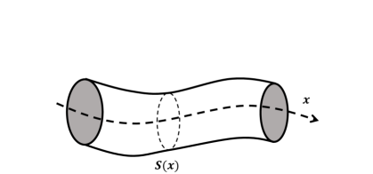
Figure 2.1: Artery as a compliant tube.

The object to model is a simplification of an artery as a compliant cylinder, illustrated in figure 2.1. We will start from a 3D reasoning and we will be making assumptions and simplifications until we arrive to the one-dimensional version of the equations. This way of modelling non-rigid arteries was presented in $2003$ by Sherwin et al. in [104] and [103].

The rest of the chapter will consist on motivating and detailing the main assumptions of the model. As we will see, a system of partial differential equations will appear, and each one of the equations will be detailed in different subsections. Before presenting them, we start with the notation and the main variables.

2.1 Governing equations

The first simplification will be to assume that the local curvature of the artery is small enough so we can indeed reduce the problem to one dimension. If we denote by $S(x)$ a cross section (we can think of it as a slice of the artery) we define

$$A(x,t)=\int_{S(x)}\mathrm{d}\sigma,$$ (2.1)

as the area of the cross section $S$;

$$u(x,t)=\frac{1}{A(x,t)}\int_{S(x)}\hat{u}(x,t)\mathrm{d}\sigma,$$ (2.2)

as the average velocity over the cross section where $\hat{u}(x,t)$ denote the value of velocity within a constant $x$-section; and

$$p(x,t)=\frac{1}{A(x,t)}\int_{S(x)}\hat{p}(x,t)\mathrm{d}\sigma,$$ (2.3)

as the internal pressure over the cross section where $\hat{p}(x,t)$ denote the value of pressure within a constant $x$-section. As it is usual in the literature, $x$ will denote the spatial coordinate and $t$ the temporal one. We remark that in order to avoid a cumbersome notation, if no confusion is added, some arguments of the functions could be avoided. Hence, in some places of this work we could write $A,u$ and $p$ for the functions previously presented. This will allow us to treat them as variables. We will also assume that the blood is an incompressible and Newtonian fluid and so the density $\rho$ and dynamic viscosity $\mu$ are constant.

Finally, for the derivation of the dynamics equations we introduce the dependent variable

$$Q(x,t)=A(x,t)u(x,t),$$ (2.4)

that will represent the volume flux at a given section. Therefor, since we have three variables, $A,u$ and $p$, or equivalently $A,Q$ and $p$, we need three equations to relate them. The first two will be conservative equations, i.e., equations that express the conservation of some quantity. The third equation will be the responsible for modelling the artery as an elastic material.

2.1.1 Continuity equation

Here we use the fluid dynamics’ continuum hypothesis what is an idealisation of continuum mechanics under which fluids can be treated as continuous, even though, on a microscopic scale, they are composed of molecules. Under the continuum assumption, macroscopic properties such as density, pressure, and velocity are taken to be well-defined at infinitesimal volume elements — small in comparison to the characteristic length scale of the system, but large in comparison to molecular length scale. Fluid properties can vary continuously from one volume element to another and they are averaged values of the molecular properties.

With this, if we take one portion of the artery as our control volume, conservation of mass requires that, if there are nor sources neither sinks, nothing disappears spontaneously, i.e., the rate of change of mass within the control volume is only due to what comes into the artery portion minus what comes out of this portion (assuming impermeable walls too). If this control volume has length $l$, we can write it as

$$V(t)=\int_{0}^{l}A(x,t)\mathrm{d}x,$$ (2.5)

and hence, due to the reasoning made before, we can write the rate of change of mass (or volume, actually) as

$$\rho\frac{\partial V(t)}{\partial t}=\rho(Q(0,t)-Q(l,t)).$$ (2.6)

We have corrected the equation with the density of the blood $\rho$ for completeness, although in our case it will have no effect. If $\rho$ depended on time, for example, this could not be simplified (we would be dealing with a compressible fluid). Now, we can rewrite this expression using the definition of $V(t)$ and the fundamental theorem of Calculus as

$$\rho\frac{\partial}{\partial t}\int_{0}^{l}A(x,t)\mathrm{d}x+\rho\int_{0}^{l}\frac{\partial Q(x,t)}{\partial x}\mathrm{d}x=0.$$ (2.7)

We have no issues in doing this since all the functions we are considering (amplitude $A$, velocity $u$ and flux $Q$) are smooth enough due to its physical meaning to integrate them and take derivatives. If we assume $l$ does not depend on time, we can take the derivative with respect to $t$, inside the integral to arrive to

$$\int_{0}^{l}\frac{\partial A}{\partial t}+\frac{\partial Q}{\partial x}\mathrm{d}x=0.$$ (2.8)

We have no problems in deriving inside the integral symbol due to the smoothness of the functions involved. Since the control volume is arbitrary, the integrand of the above equation must be zero. We therefor obtain the differential one-dimensional mass conservation equation

$$\frac{\partial A}{\partial t}+\frac{\partial Q}{\partial x}\equiv\frac{\partial A}{\partial t}+\frac{\partial(uA)}{\partial x}=0.$$ (2.9)

2.1.2 Momentum equation

The second equation comes from the concept of momentum of Newtonian dynamics. Analogously as we have done with the mass-conservation equation (or continuity equation), the momentum equation states that the rate of change of momentum within the control volume plus the net flux of momentum out the control volume is equal to the applied forces on the control volume. Again, we have to weight with the blood density since the flux is involved. This is,

$$\frac{\partial}{\partial t}\int_{0}^{l}\rho Q\mathrm{d}x+\rho\left(Q(l,t)u(l,t)-Q(0,t)u(0,t)\right)=F,$$ (2.10)

where $F$ is the set of forces acting in the control volume. In this term we have to take into account the friction with the walls, the pressure of the flow against the walls and the force at the inlet minus the force at the outlet. Since the pressure is force per unit area, we can write this term as

$$F(t)=\underbrace{p(0,t)A(0,t)}_{\textrm{Force at the inlet}}-\underbrace{p(l,t)A(l,t)}_{\textrm{Force at the outlet}}+\underbrace{\int_{0}^{l}\int_{\partial S}\hat{p}n_{x}\mathrm{d}s\mathrm{d}x}_{\textrm{Pressure against the walls}}+\underbrace{\int_{0}^{l}f\mathrm{d}x}_{\textrm{Friction}},$$ (2.11)

where $\partial S$ is the boundary of section $S$, $n_{x}$ is the $x$-component of the surface normal and $f$ represents the friction force per unit length. The side wall pressure force given by the double integral can be simplified if we assume constant sectional pressure and we treat the tube as axisymmetric:

$$\int_{0}^{l}\int_{\partial S}\hat{p}n_{x}\mathrm{d}s\mathrm{d}x=\int_{0}^{l}p\frac{\partial A}{\partial x}\mathrm{d}x.$$ (2.12)

Putting everything altogether we arrive to the control-volume statement of momentum conservation

$$\begin{split}&\frac{\partial}{\partial t}\int_{0}^{l}\rho Q\mathrm{d}x+\rho(Q(l,t)u(l,t)-Q(0,t)u(0,t))\\ =&p(0,t)A(0,t)-p(l,t)A(l,t)+\int_{0}^{l}\left(p\frac{\partial A}{\partial x}+f\right)\mathrm{d}x.\end{split}$$ (2.13)

As we have done before, using the fundamental theorem of Calculus and assuming $l$ is independent of time and $\rho$ is constant, we obtain

$$\int_{0}^{l}\left[\rho\left(\frac{\partial Q}{\partial t}+\frac{\partial(Qu)}{\partial x}\right)+\frac{\partial(pA)}{\partial x}-p\frac{\partial A}{\partial x}-f\right]\mathrm{d}x=0.$$ (2.14)

Since this equation is satisfied for an arbitrary control volume, the integrand must be zero, so the equation has the form

$$\frac{\partial Q}{\partial t}+\frac{\partial(Qu)}{\partial x}=-\frac{A}{\rho}\frac{\partial p}{\partial x}+\frac{f}{\rho}.$$ (2.15)

Finally, due to the appearance of $u^{2}$ in (2.15) ($Qu=Au^{2}$), it is convenient to introduce the Coriolis coefficient $\alpha$ as a correction factor for the non-linearity of the momentum, so as to satisfy

$$\alpha(x,t)=\frac{\int_{S}\hat{u}\mathrm{d}\sigma}{Au^{2}},$$ (2.16)

where $\hat{u}$ stands for velocity within a constant $x$-section. Although in some papers such as [104] this coefficient is simplified to $\alpha=1$, which means a flat profile, some others as [119] set them to $\alpha=4/3$ for a parabolic profile. With this, the final conservation of momentum equation reads

$$\frac{\partial Q}{\partial t}+\frac{\partial(\alpha Qu)}{\partial x}=-\frac{A}{\rho}\frac{\partial p}{\partial x}+\frac{f}{\rho}.$$ (2.17)

2.1.3 The tube laws

We recall that we have three variables, $A,u$ and $p$ (or the combinations using the volume flux $Q$) and up to this moment only two equations: mass and momentum conservation. Consequently, to close the system given by equations (2.9) and (2.17) either we need one equation more or we have to remove one variable. This is commonly done defining a relationship, either differential or algebraic, between pressure and amplitude (known as the local tube law). One could expect one well-established equation, as is the case of the conservation equations but, to the best of our knowledge there is no scientific agreement at this point. The reason of this, is because they are generally simplifications of the physical reality, so depends on the author which assumptions to make. Other ones leave free parameters in order to fit them with experimental data and other group of authors uses expressions purely mathematical. In this part we will make a brief review of some of the most important ones.

Before exposing them one clarification must be done. Depending on the reference, we will be using an initial pressure $p_{0}(x)=p(x,0)$, a reference pressure $p_{\textrm{ref}}(x,t)$, an external pressure $p_{\textrm{ext}}(x,t)$ or none of them. These usually appear as a difference with the current pressure so the idea is that we are in a non-equilibrium situation. Some authors assume that at the beginning of the simulation we are in equilibrium so they use $p_{0}(x)$; other models embrace other pressures such as atmospheric pressure (to distinguish if the artery is in vertical position or not) or they treat it as a different term ($p_{\textrm{ext}}(x,t)$) and most of them assume that the initial/reference pressure is zero in order to simplify. This is not a great issue since the reasoning is the same and for further simulations we will simplify these terms.

1. Historically, one of the first approaches has been to assume that the cross-sectional area is a linear function of pressure and also that changes in area are relatively small. That is,

   $$A(x,t)=A_{0}(x)+(p(x,t)-p_{0}(x))C(x,t)$$ (2.18)

   with

   $$|(p(x,t)-p_{0}(x))C(x,t)|\ll A_{0}(x)$$ (2.19)

   where $C(x,t)=\left.\frac{\partial A(x,t)}{\partial p(x,t)}\right|_{A_{0}(x)}$ is the vessel compliance per unit length,
   $p_{0}(x)=p(x,0)$ and $A_{0}(x)=A(x,0)$. These equations, together with experimental values of $C(x,t)$ (assumed constant) can be found in [96].

2. We can think of the previous expression as a Taylor expansion neglecting terms higher than first order. The natural question is if it is possible to get a higher order and, indeed, this has been studied back in $1986$ in [93]. They presented the equation

   $$A(x,t)=A_{0}(x)\left[1+C_{0}(p(x,t)-p_{0}(x))+C_{1}(p(x,t)-p_{0}(x))^{2}\right],$$ (2.20)

   which is particularly convenient for numerical manipulation.

3. In [104] and [103], Sherwin et al. assumed a thin wall tube where each section is independent of the others. This model is based on linear elasticity where, using Hooke’s law (first formulated in [55]) for continuous media we have that

   $$\sigma=E\varepsilon$$ (2.21)

   being $\sigma$ the stress, $\varepsilon$ the strain and $E$ the Young’s modulus. We recall that, despite they are actually tensors, the stress can be defined as a physical quantity that expresses the internal forces that neighbouring particles of a continuous material exert on each other, while strain is the measure of the deformation of the material. Young’s modulus characterise the stiffness of an elastic material.

   Let us denote the radius of the artery by $R(x,t)$ and $R_{0}(x)=R(x,0)$. Here $h_{0}(x)$ will be used to denote the vessel-wall thickness and sectional area at the equilibrium state $(p,u)=(p_{\textrm{ref}},0)$, where $p_{\textrm{ref}}$ is the reference pressure. We assume a cross section of a vessel with a thin wall ($h\ll R$), an isotropic, homogeneous, incompressible arterial wall that it deforms axisymmetrically with each circular cross-section independently of the others. Making these assumptions, we can express the strain as

   $$\varepsilon=\frac{R-R_{0}}{(1-\nu^{2})R_{0}},$$ (2.22)

   where $\nu(x)$ is the other elasticity parameter, Poisson’s ratio. It is defined as the ratio of transverse contraction strain to longitudinal extension strain in the direction of stretching force, so along with Young’s modulus one can univocally determine the properties of a (linear) elastic material. By Young-Laplace’s law, assuming there is not external pressure we can relate the pressure with the stress as

   $$p=\frac{h_{0}\sigma}{\pi R}.$$ (2.23)

   Combining the previous equations we arrive to the tube law

   $$p(x,t)=p_{\textrm{ext}}+\beta(x)\left(\sqrt{A(x,t)}-\sqrt{A_{0}(x)}\right),$$ (2.24)

   where

   $$\beta(x)=\frac{\sqrt{\pi}h_{0}(x)E(x)}{\left(1-\nu(x)^{2}\right)A_{0}(x)}$$ (2.25)

   is the parameter embracing the material properties and $p_{\textrm{ext}}$ is the external pressure. There are no problems with the denominator since in most of the materials $\nu(x)\in[0,0.5]$ and, although in capillaries the amplitude $A_{0}$ is very small, the wall thickness $h_{0}$ is too. Nevertheless, if this is the case, we must pay attention because of computational issues.

4. Another approach, similar to the previous model, is to assume a linear pressure-area constitutive relation, as in [111], and hence the pressure is proportional to arterial amplitude difference, that is

   $$p(x,t)=\gamma(x,t)(A(x,t)-A_{0}(x))$$ (2.26)

   where $\gamma$ is a proportionality coefficient. To the best of our knowledge this coefficient has no explicit physical meaning.

5. All of these models can be found in a more general way in a recent review (see [119]). Here, Toro wrote the tube law as

   $$p(x,t)=\psi(A;K,A_{0}),$$ (2.27)

   where

   $$\psi(A;K,A_{0})=K(x)\phi(A,A_{0})$$ (2.28)

   and

   $$\phi(A,A_{0})=\left[\left(\frac{A(x,t)}{A_{0}(x)}\right)^{m}-\left(\frac{A(x,t)}{A_{0}(x)}\right)^{n}\right],$$ (2.29)

   where $m,n$ and $K(x)$ are free parameters and a function. We can recover equation (2.24) by setting $m=1/2$, $n=0$ and

   $$K(x)=\sqrt{\frac{\pi}{A_{0}(x)}}\left(\frac{h_{0}(x)E(x)}{1-\nu^{2}(x)}\right).$$ (2.30)

   In this case, we would have that $\beta(x)=K(x)/\sqrt{A_{0}(x)}$. If it is not specified, we can always replace $p(x,t)$ by $p(x,t)-p_{\textrm{ref}}(x,t)$ because in most of the models the reference pressure is set to $0$ for simplicity.

   
   

   Up to this point, the tube laws presented have been based on a purely elastic behaviour of the artery wall. Another parallel line of work has been to consider the artery wall as a viscoelastic material. For the arterial wall (or viscoelastic solids in general), when a fixed stress is loaded, the wall keeps extending gradually (creeping) after an instantaneous extension. The main issue for the simulation of viscoelastic materials is the significant increase of theoretical and computational complexity (both in running time as in code development) but, for completeness, we present some of the most used models. We will do it in a more enumerating way, since the deduction of all the equations is out of the scope of this work.

6. We can find a complex formulation of viscoelasticity for blood vessels back in $1970$ in [126]. The following tube law of the generalised viscoelastic model can be derived using knowledge of solid mechanics:

   $$p(x,t)=\frac{1}{C(x,t)}\left[A(x,t)-A_{0}(x)+\int_{0}^{t}\sum_{i=1}^{n}f_{i}e^{-(t-u)/\tau_{i}}\frac{\partial A(x,u)}{\partial t}\mathrm{d}u\right]$$ (2.31)

   where $C(x,t)=\left.\frac{\partial A(x,t)}{\partial p(x,t)}\right|_{A_{0}(x)}$. The viscoelastic property of the tube wall is reflected in the dynamic viscoelasticity parameters $f_{i}$ and relaxation time parameter $\tau_{i}$. It is possible to determine the term number $n$ from the viscoelastic characteristics of the material.

7. A widely used viscoelastic model is Kelvin-Voigt model which writes

   $$\sigma(t)=E\varepsilon(t)+\phi\frac{\partial\varepsilon(t)}{\partial t},$$ (2.32)

   being $\phi$ a coefficient for the viscosity of the material. We note that if $\phi=0$ we have a linear relationship and hence we recover the elastic model. If we suddenly apply some constant stress $\sigma_{0}$ to a Kelvin–Voigt material, then the deformations would approach the deformation for the pure elastic material $\sigma_{0}/E$ with the difference decaying exponentially:

   $$\varepsilon(t)=\frac{\sigma_{0}}{E}\left(1-e^{-\lambda t}\right),$$ (2.33)

   where $\lambda$ can be interpreted as the rate of relaxation

   $$\lambda=\frac{E}{\phi}.$$ (2.34)

   Hence, it is the description of a elastic material but with some delay. This is the reason why it is the description of a viscoelastic material.

   Using the same reasoning as in the third model we get the tube law

   $$p=\beta\left(\sqrt{A}-\sqrt{A_{0}}\right)+\nu_{s}\frac{\partial A}{\partial t},$$ (2.35)

   with stiffness coefficient

   $$\beta=\frac{\sqrt{\pi}Eh}{(1-\nu^{2})A_{0}}$$ (2.36)

   and viscosity coefficient

   $$\nu_{s}=\frac{\sqrt{\pi}\phi h}{2(1-\nu^{2})\sqrt{A_{0}}A}.$$ (2.37)

   This model was first used in by Čanić et al. in [16] (although in a more general way).

8. Finally, one of the most novel approaches has been to use the concept of fractional derivative. This branch of calculus consider not only the first, second… derivatives, but “intermediate” ones. One of the most used definitions (specially oriented to computational purposes) starts with the basic definition of derivative:

   $$\begin{split}f^{\prime}(x)&=\lim_{h\to 0}\frac{f(x+h)-f(x)}{h},\\ f^{\prime\prime}(x)&=\lim_{h\to 0}\frac{f^{\prime}(x+h)-f^{\prime}(x)}{h}=\lim_{h\to 0}\frac{f(x+2h)-2f(x+h)+f(x)}{h^{2}},\\ &\vdots\\ f^{(n)}(x)&=\lim_{h\to 0}\frac{\sum_{0\leq m\leq n}(-1)^{m}\binom{n}{m}f(x+(m-n)h)}{h^{n}}.\end{split}$$ (2.38)

   In order to achieve real (even complex) values of the derivative’s degree we replace the factorial with the Euler’s gamma function (which returns the factorial for integer values). With some algebra we arrive to:

   $$\begin{split}\mathrm{D}^{\alpha}f(x)&=\lim_{h\to 0}h^{-\alpha}\sum_{m=0}^{\frac{x-a}{h}}\frac{(-1)^{m}\Gamma(\alpha+1)}{\Gamma(m+1)\Gamma(\alpha-m+1)}f(x-mh)\\ &=\lim_{n\to\infty}\left(\frac{n}{x-a}\right)^{\alpha}\sum_{m=0}^{n}\frac{(-1)^{m}\Gamma(\alpha+1)}{\Gamma(m+1)\Gamma(\alpha-m+1)}f\left(x-m\left(\frac{x-a}{n}\right)\right),\end{split}$$ (2.39)

   where now $\alpha\in\mathbb{C}$ and $a<x$ is the point from where the derivative corresponding to $x$ will be calculated. This definition is called the Grünwald-Letnikov formula, first used in [74]. It is not the unique definition, since there are more than thirty (see [18]) and some of them are not even equivalent. Nevertheless, what all of them have in common is that they have some “memory”, in the sense that previous values of the derivative’s degree, affect the current value. Using this idea, Perdikaris et al. modelled arterial viscoelasticity with fractional calculus and they run its interaction with blood flow in [89]. For this, they use the Grünwald-Letnikov formula in a recursive way:

   $$D_{t}^{\alpha}f(t)=\lim_{\Delta t\to 0}\Delta t^{-\alpha}\sum_{k=0}^{\infty}GL_{k}^{\alpha}f(t-k\Delta t),$$ (2.40)

   $$GL_{k}^{\alpha}=\frac{k-\alpha-1}{k}GL_{k-1}^{\alpha}$$ (2.41)

   with $GL_{0}^{\alpha}=1$ and $t-k\Delta t$ must be in the domain of $f$. The fractional stress-strain relation reads as

   $$\sigma(t)+\tau_{\sigma}^{\alpha}D_{t}^{\alpha}\sigma(t)=E\left[\varepsilon(t)+\tau_{\varepsilon}^{\alpha}D_{t}^{\alpha}\varepsilon(t)\right].$$ (2.42)

   And, as before

   $$\sigma=\frac{R(p-p_{\textrm{ext}})}{h_{0}}\qquad\textrm{and}\qquad\varepsilon=\frac{R-R_{0}}{(1-\nu^{2})R_{0}}.$$ (2.43)

   So, replacing the equations of (2.43) and the expression of fractional derivative of (2.40) in the stress-strain relationship (2.42) we arrive to

   $$\begin{split}p(x,t)=\frac{1+\tau_{\varepsilon}^{\alpha}\Delta t^{-\alpha}}{1+\tau_{\sigma}^{\alpha}\Delta t^{-\alpha}}p^{E}(x,t)+\frac{\Delta t^{-\alpha}}{1+\tau_{\sigma}^{\alpha}\Delta t^{-\alpha}}\\ \times\sum_{k=0}^{\infty}GL_{k}^{\alpha}\left[\tau_{\varepsilon}^{\alpha}p^{E}(t-k\Delta t)-\tau_{\sigma}^{\alpha}p(t-k\Delta t)\right]\end{split}$$ (2.44)

   where $p^{E}$ correspond to the elastic pressure contribution

   $$p^{E}(x,t)=\left(\frac{\tau_{\varepsilon}}{\tau_{\sigma}}\right)^{\alpha}\beta\left(\sqrt{A}-\sqrt{A_{0}}\right).$$ (2.45)

   The parameters $\tau_{\varepsilon},\tau_{\sigma}$ and the fractional exponent $\alpha$ have to be properly chosen each case. We notice that for the case $\tau_{\sigma}^{\alpha}=0$, $\tau_{\varepsilon}^{\alpha}=1/E$ and $\alpha=1$ we recover the Kelvin-Voigt model.

We have provided a briefly overview of several ways of modelling the elastic or viscoelastic behaviour of the arterial wall, since the seventies up to the most recent models. We can visually check the appearing of these ideas in figure 2.2.

 M7 1970 Westerhof M1 1974 Raines M2 1986 Porenta M3 2003 Sherwin

  M5 2016 Toro M6 2006 Čanić M8 2014 Capelas de Oliveira M4 2013 Sochi

Figure 2.2: Chronology of the models presented on the tube law subsection.

With this, we have shown in this chapter the statement of our problem with some of the most important options for the tube law. Although we will remark it in the following sections, due to its usefulness and because it is not purely phenomenological, we will use the third model, i.e., the purely elastic wall model where the proportionality constant has a clear physical sense. With this, in the next chapter we will use the aforementioned Navier-Stokes problem and with theory of partial differential equations (specifically, hyperbolic problems) we will prove some statements that will be useful for practical cases.

Chapter 3 Theoretical analysis applied to the Navier-Stokes problem

In this chapter we will use some mathematical tools to analyse the system of partial differential equations presented in the previous chapter. This analysis will be mainly based on a widely known (specially in engineering areas) method, the so-called method of characteristics. Although it is sometimes used as a numerical method, we will use the theoretical background of it (explained in section 3.1) to prove some useful theorems in the section 3.2.

3.1 Method of characteristics

Since the rest of the chapter is based on the method of characteristics, we will use this section to explain the main ideas of this method and apply it to our problem.

The method of Riemann characteristics has been used for more than a century to describe linear and nonlinear waves propagating in a medium [100]. The main useful properties of this method, as are discussed in [87], are that it may be applied to both linear and nonlinear systems; that it may be applied equally well to solids, liquids, and gases; and that it provides a clear picture of the causal relations governing system behaviour. The method of characteristics was first developed by Riemann in an article published in $1860$. Riemann limits himself to consideration of gases and begins with a discussion of the ideal gas law. He then progresses to a development of the method of characteristics and a discussion of applications of the method.

Riemann’s work is built upon previous work on finite amplitude waves in air. An important contribution was made by Poisson [92] whose $1808$ article showed that the wave velocity is the sum of the sound speed and the mean flow velocity. Properties of waves of finite amplitude were discussed in $1860$ by Earnshaw [32], but only for progressive waves.

Very roughly, a characteristic is a propagation path: a path followed by some entity, such a geometrical form or a physical disturbance when this entity is propagated. Thus, a “gridiron” of roads could be considered as propagation paths, as is shown in figure 3.1(a). With this very intuitive notion of characteristic (extracted from [1]), the two families of lines correspond to two families of characteristics, usually named forward characteristic and backward characteristic.

(a) Characteristic curves with constant slope.

(b) (Forward) characteristic curves with variable slope.

(c) Formation of a shock wave.

Figure 3.1: Scheme of different types of characteristic curves.

With this method we want to transform a partial differential equation (or a system of equations) into an ordinary differential equation (or a system of equations). The usual way of achieving this is making linear combinations of certain terms choosing properly the multipliers. In the following subsection we will explain the general procedure for the case of a quasi-linear system with two variables. The problem with this derivation of the method is that it is based on calculus of variations where infinitesimal quantities are treated as manipulable entities. This approach is very common in engineering and physics but, regarding its rigour, it is not well appreciated in some mathematical fields. Nevertheless, for completeness and for historical reasons we will show this procedure.

3.1.1 Derivation of the method via calculus of variations

In this subsection we will follow the notation and discussion of the $15$^th chapter of [97] written by Lister.

The general form of a quasi-linear system of equations for the case of two independent variables $x,y$ and two dependent variables $u,v$ can be written as a system of two equations, $L_{1}$ and $L_{2}$:

$$L_{1}:A_{1}u_{x}+B_{1}u_{y}+C_{1}v_{x}+D_{1}v_{y}+E_{1}=0$$ (3.1)

$$L_{2}:A_{2}u_{x}+B_{2}u_{y}+C_{2}v_{x}+D_{2}v_{y}+E_{2}=0$$ (3.2)

where $A_{1},A_{2},\dots,E_{2}$ are known functions of $x,y,u,v$.

In the following considerations, it is assumed that all the functions introduced above are continuous and possess as many continuous derivatives as may be required. Consider a linear combination of $L_{1}$ and $L_{2}$:

$$\begin{split}L=\lambda_{1}L_{1}+\lambda_{2}L_{2}=&(\lambda_{1}A_{1}+\lambda_{2}A_{2})u_{x}+(\lambda_{1}B_{1}+\lambda_{2}B_{2})u_{y}+(\lambda_{1}C_{1}+\lambda_{2}C_{2})v_{x}\\ &+(\lambda_{1}D_{1}+\lambda_{2}D_{2})v_{y}+(\lambda_{1}E_{1}+\lambda_{2}E_{2}).\end{split}$$ (3.3)

Now, if $u=u(x,y)$ and $v=v(x,y)$ are solutions to (3.1) and (3.2) then

$$\mathrm{d}u=\frac{\partial u}{\partial x}\mathrm{d}x+\frac{\partial u}{\partial y}\mathrm{d}y,\qquad\mathrm{d}v=\frac{\partial v}{\partial x}\mathrm{d}x+\frac{\partial v}{\partial y}\mathrm{d}y.$$ (3.4)

The differential expression $L$ can be written in the form

$$\mathrm{d}xL=(\lambda_{1}A_{1}+\lambda_{2}A_{2})\mathrm{d}u+(\lambda_{1}C_{1}+\lambda_{2}C_{2})\mathrm{d}v+(\lambda_{1}E_{1}+\lambda_{2}E_{2})\mathrm{d}x$$ (3.5)

if the constants $\lambda_{1}$ and $\lambda_{2}$ are chosen so that

$$\frac{\mathrm{d}x}{\mathrm{d}y}=\frac{\lambda_{1}A_{1}+\lambda_{2}A_{2}}{\lambda_{1}B_{1}+\lambda_{2}B_{2}}=\frac{\lambda_{1}C_{1}+\lambda_{2}C_{2}}{\lambda_{1}D_{1}+\lambda_{2}C_{2}}.$$ (3.6)

In this case, in the differential expression $L$, the derivatives of $u$ and those of $v$ are combined so that their derivatives are in the same direction, namely, $\mathrm{d}y/\mathrm{d}x$. This direction is called a characteristic direction.

From equation (3.6), the ratio $\lambda_{1}/\lambda_{2}$ can be obtained:

$$-\frac{\lambda_{1}}{\lambda_{2}}=\frac{A_{2}\mathrm{d}y-B_{2}\mathrm{d}x}{A_{1}\mathrm{d}y-B_{1}\mathrm{d}x}=\frac{C_{2}\mathrm{d}y-D_{2}\mathrm{d}x}{C_{1}\mathrm{d}y-D_{1}\mathrm{d}x}$$ (3.7)

hence

$$a(\mathrm{d}y)^{2}-2b\ \mathrm{d}x\mathrm{d}y+c(\mathrm{d}x)^{2}=0.$$ (3.8)

Here,

$$a =A_{1}C_{2}-A_{2}C_{1},$$ (3.9)

$$2b =A_{1}D_{2}-A_{2}D_{1},$$ (3.10)

$$c =B_{1}D_{2}-B_{2}D_{1}.$$ (3.11)

For the case of hyperbolic partial differential equations, two distinct roots of the quadratic equation (3.8) exist. Therefor

$$b^{2}-ac>0.$$ (3.12)

This excludes the exceptional case of all three coefficients vanishing. Moreover, it is assumed for convenience that

$$a\neq 0.$$ (3.13)

The latter condition can always be satisfied, if necessary, by introducing new coordinates instead of $x$ and $y$. Consequently, $\mathrm{d}x\neq 0$ for a characteristic direction $(\mathrm{d}x,\mathrm{d}y)$ as seen from (3.8); thus the slope

$$\zeta=\frac{\mathrm{d}y}{\mathrm{d}x}$$ (3.14)

can be introduced, and $\zeta$ satisfies the equation:

$$a\zeta^{2}-2b\zeta+c=0.$$ (3.15)

This equation has two different real solutions $\zeta_{+}$ and $\zeta_{-}$,

$$\zeta_{+}\neq\zeta_{-}.$$ (3.16)

Thus, at the point $(x,y)$, the two different characteristic directions are given by:

$$\frac{\mathrm{d}y}{\mathrm{d}x}=\zeta_{+},\quad\frac{\mathrm{d}y}{\mathrm{d}x}=\zeta_{-}.$$ (3.17)

Since $a,b$ and $c$ are in general functions of $u,v,x$ and $y$, $\zeta_{+}$ and $\zeta_{-}$ will also be functions of these quantities:

$$\frac{\mathrm{d}y}{\mathrm{d}x}=\zeta_{+}(x,y,u,v),\quad\frac{\mathrm{d}y}{\mathrm{d}x}=\zeta_{-}(x,y,u,v).$$ (3.18)

Once a solution $u(x,y),v(x,y)$ of (3.1) and (3.2) has been obtained, equations
(3.18) become two separate ordinary differential equations of the first order. These ODEs define two one-parameter families of characteristic curves (often abbreviated to characteristics), in the $(x,y)$ plane, belonging to this solution $u(x,y),v(x,y)$. These two families form a curvilinear coordinate net (as could be figure 3.1(b)).

If $\zeta_{+}$ and $\zeta_{-}$ are functions of $x$ and $y$ only, then

$$\frac{\mathrm{d}y}{\mathrm{d}x}=\zeta_{+}(x,y),\quad\frac{\mathrm{d}y}{\mathrm{d}x}=\zeta_{-}(x,y),$$ (3.19)

and it is not necessary to find a solution to (3.1) and (3.2) in order to find the equations of the characteristics; hence the problem is simplified.

Substituting the solutions (3.17) into the expressions for $\lambda_{1}/\lambda_{2}$ given in (3.7) yields

$$\frac{\lambda_{1}}{\lambda_{2}}=-\frac{A_{2}\zeta_{+}-B_{2}}{A_{1}\zeta_{+}-B_{1}},\quad\frac{\lambda_{1}}{\lambda_{2}}=-\frac{A_{2}\zeta_{-}-B_{2}}{A_{1}\zeta_{-}-B_{1}}.$$ (3.20)

Finally, combining (3.20) and (3.5) gives

$$F\mathrm{d}u+(a\zeta_{+}-G)\mathrm{d}v+(K\zeta_{+}-H)\mathrm{d}x =0,$$ (3.21)

$$F\mathrm{d}u+(a\zeta_{-}-G)\mathrm{d}v+(K\zeta_{-}-H)\mathrm{d}x =0,$$ (3.22)

where

$$F =A_{1}B_{2}-A_{2}B_{1}, G =B_{1}C_{2}-B_{2}C_{1},$$

$$K =A_{1}E_{2}-A_{2}E_{1}, H =B_{1}E_{2}-B_{2}E_{1}.$$

Thus, the following four characteristic equations have been obtained:

$$\mathrm{d}y-\zeta_{+}\mathrm{d}x =0$$ (3.24)

$$F\mathrm{d}u+(a\zeta_{+}-G)\mathrm{d}v+(K\zeta_{+}-H)\mathrm{d}x =0$$ (3.25)

$$\mathrm{d}y-\zeta_{-}\mathrm{d}x =0$$ (3.26)

$$F\mathrm{d}u+(a\zeta_{-}-G)\mathrm{d}v+(K\zeta_{-}-H)\mathrm{d}x =0$$ (3.27)

Equations (3.24)–(3.27) are of a particularly simple form, inasmuch as each equation contains only total derivatives of all the variables.

According to the derivation, every solution of the original system (3.1) and (3.2) satisfies the system (3.24)–(3.27). Courant and Friedrichs showed that the converse is also true in [23].

At this point we could apply the previous reasoning to our case (previously checking the hyperbolicity) but we will avoid this path. The reasoning followed is more typical in physics’ and engineering areas, but we can provide more rigour to this method. The method of characteristics can also be achieved by means of linear algebra and standard calculus: we will dedicate the following subsections to the derivation of the method in this way. This will also provide the notation and the tools for a posterior analysis of the problem.

3.1.2 Setting of the Navier-Stokes system

First of all, let us manipulate the expression of the momentum equation (2.17) for convenience (the left-hand side):

$$\begin{split}\frac{\partial Q}{\partial t}+\frac{\partial\alpha Qu}{\partial x}&=\frac{uA}{\partial t}+\frac{\partial\overbrace{\alpha u^{2}A}^{(\alpha uA)u}}{\partial x}=A\frac{\partial u}{\partial t}+u\frac{\partial A}{\partial t}+u\frac{\partial\alpha uA}{\partial x}+\alpha uA\frac{\partial u}{\partial x}\\ &=A\frac{\partial u}{\partial t}+u\frac{\partial A}{\partial t}+u\frac{\partial\alpha uA}{\partial x}+\alpha uA\frac{\partial u}{\partial x}+u\frac{uA}{\partial x}-u\frac{uA}{\partial x}\\ &=u\frac{\partial A}{\partial t}+u\frac{\partial uA}{\partial x}+u\frac{\partial\alpha uA}{\partial x}-u\frac{\partial\alpha uA}{\partial x}+\alpha uA\frac{\partial u}{\partial x}\\ &=u\left\{\frac{\partial A}{\partial t}+\frac{\partial uA}{\partial x}\right\}+u\frac{\partial(\alpha-1)uA}{\partial x}+A\left\{\frac{\partial u}{\partial t}+\alpha u\frac{\partial u}{\partial x}\right\}.\end{split}$$ (3.28)

The first term is the mass conservation equation (2.9) and is therefor zero. Following the simplifications made by [103] we now assume inviscid flow with a flat profile, which implies that $f=0$ and $\alpha=0$.

This will not be a big deal, since it was shown in [15] that the source term is one order of magnitude smaller than the effects of non-linear advection. Since the inviscid flow does not generate boundary layer it is physically reasonable to assume the aforementioned flat velocity profile.

Even though this might seem a crude assumption, comparison with experimental data [57] has shown that blood velocity profiles are rather flat on average. Furthermore, this assumption simplifies the analysis. However, we should stress that the methods to be presented in the following sections may be readily extended to the case $\alpha\neq 1$. Moreover, due to its wide use in the literature we will also assume the model M3) for the pressure of subsection 2.1.3.

Using this and the continuity equation (2.9) we can write the governing equations in terms of the $(A,u)$ variables as

$$\frac{\partial A}{\partial t}+\frac{\partial uA}{\partial x} =0,$$ (3.29)

$$\frac{\partial uA}{\partial t}+\frac{\partial u^{2}/2}{\partial x} =-\frac{1}{\rho}\frac{\partial p}{\partial x}.$$ (3.30)

Equivalently, we can write the system in conservative form as

$$\textbf{U}_{t}+\textbf{F}_{x}=0,$$ (3.31)

with

$$\textbf{U}=\begin{bmatrix}A\\ u\end{bmatrix},\qquad\textbf{F}=\begin{bmatrix}uA\\ \frac{u^{2}}{2}+\frac{p}{\rho}\end{bmatrix},$$ (3.32)

denoting the derivatives with subscripts. With this rearrangement of the system, we will obtain now the characteristic curves and variables.

3.1.3 Characteristic variables

The first step is to use the chain rule in the equation (2.24). Thus, we have

$$\frac{\partial p}{\partial x}=\frac{\partial p}{\partial A}\frac{\partial A}{\partial x}+\frac{\partial p}{\partial\beta}\frac{\partial\beta}{\partial x}+\frac{\partial p}{\partial A_{0}}\frac{\partial A_{0}}{\partial x}=\frac{\beta}{2\sqrt{A}}\frac{\partial A}{\partial x}+\frac{\partial p}{\partial\beta}\frac{\partial\beta}{\partial x}+\frac{\partial p}{\partial A_{0}}\frac{\partial A_{0}}{\partial x}.$$ (3.33)

Hence, we can rewrite system (3.31) in its quasi-linear form as

$$\textbf{U}_{t}+\textbf{H}\textbf{U}_{x}=\begin{bmatrix}A_{t}\\ u_{t}\end{bmatrix}+\begin{bmatrix}u&A\\ c^{2}/A&u\end{bmatrix}\begin{bmatrix}A_{x}\\ u_{x}\end{bmatrix}=\begin{bmatrix}0\\ g\end{bmatrix}=\textbf{G},$$ (3.34)

with

$$\begin{split}c^{2}&=\frac{\beta\sqrt{A}}{2\rho},\\ g&=\frac{1}{\rho}\left(-\frac{\partial p}{\beta}\frac{\partial\beta}{\partial x}+\frac{\partial p}{\partial A_{0}}\frac{\partial A_{0}}{\partial x}\right).\end{split}$$ (3.35)

To see what kind of problem we are dealing with, we look at the eigenvalues of H. We can diagonalise H as

$$\textbf{H}=\textbf{P}^{-1}\textbf{D}\textbf{P}$$ (3.36)

with

$$\textbf{P}=\begin{bmatrix}\frac{c}{A}&1\\ -\frac{c}{A}&1\end{bmatrix},\qquad\textbf{D}=\begin{bmatrix}u+c&0\\ 0&u-c\end{bmatrix}.$$ (3.37)

Now, $\textbf{D}_{11}>0$ and, since $\beta$ is usually considerably bigger than the typical blood velocities, we have that $\textbf{D}_{22}<0$. For the typical values of the parameters found in the literature we refer to appendix A. Hence, we have two real and distinct eigenvalues for the quasi-linear problem. This means that our problem is strictly hyperbolic.

We recall that we are looking for the characteristic variables, the Riemann invariants. This is equivalent to find some variables that satisfy some equation in conservative form such as equation (3.31). We do this in the following way. With the decomposition (3.36) (left eigensystem) we can reformulate the system (3.34) as

$$\textbf{U}_{t}+\textbf{H}\textbf{U}_{x}=\textbf{G}\equiv\textbf{U}_{t}+\textbf{P}^{-1}\textbf{D}\textbf{P}\textbf{U}_{x}=\textbf{G}\equiv\textbf{P}\textbf{U}_{t}+\textbf{D}\textbf{P}\textbf{U}_{x}=\textbf{P}\textbf{G}.$$ (3.38)

If P were a constant matrix with respect to the solution variables, we could rename $\textbf{P}\textbf{U}=:\textbf{W}$ so we could get a conservative system. Following this idea, we are looking for W such that

$$\textbf{W}_{t} =\textbf{P}\textbf{U}_{t},$$ (3.39)

$$\textbf{W}_{x} =\textbf{P}\textbf{U}_{x},$$ (3.40)

where we recall that the matrix P depends on $A$. On the other hand, by the chain rule we have

$$\frac{\partial\textbf{W}(A,u)}{\partial t}=\textbf{W}_{A}A_{t}+\textbf{W}_{u}u_{t}=\left(\nabla\textbf{W}\right)\textbf{U}_{t},$$ (3.41)

being $\nabla\textbf{W}$ the gradient of W (the procedure with $\textbf{W}_{x}$ is the same). Therefor

$$\textbf{P}\textbf{U}_{x} =\textbf{W}_{x}=(\nabla\textbf{W})\textbf{U}_{x},$$ (3.42)

$$\textbf{P}\textbf{U}_{t} =\textbf{W}_{t}=(\nabla\textbf{W})\textbf{U}_{t}$$ (3.43)

which implies that

$$\textbf{P}=\nabla\textbf{W}$$ (3.44)

if and only if

$$\frac{\partial W_{1}}{\partial A} =\frac{c}{A}, \frac{\partial W_{1}}{\partial u} =1,$$ (3.45)

$$\frac{\partial W_{2}}{\partial A} =-\frac{c}{A}, \frac{\partial W_{2}}{\partial u} =1.$$ (3.46)

Integrating we arrive to:

$$\begin{split}W_{1,2}&=\int_{u_{\textrm{ref}}}^{u}\mathrm{d}u\pm\int_{A_{\textrm{ref}}}^{A}\frac{c}{A}\mathrm{d}A=u-u_{\textrm{ref}}\pm\int_{A_{\textrm{ref}}}^{A}\frac{c}{A}\mathrm{d}A\\ &=u\pm 4\sqrt{\frac{\beta}{2\rho}}A^{1/4},\end{split}$$ (3.47)

where $(u_{\textrm{ref}},A_{\textrm{ref}})=(0,0)$ is taken as the reference state. This assumption has been made previously in [104]. The characteristic variables given by equation (3.47) are also Riemann invariants of the system (3.29) and (3.30) in terms of the $(A,u)$ variables. We have achieved an explicit expression for the characteristic curves. This will allow us to use them and to check some interesting properties for practical uses. Among others, in section 3.2 we will be able to use these expressions to check the existence of a global smooth solution.

Finally, since in a coherent solution $\beta(x,t)$ is always positive, we can write the variables $(A,u)$ in terms of $(W_{1},W_{2})$ as

$$A=\left(\frac{W_{1}-W_{2}}{4}\right)^{4}\left(\frac{\rho}{2\beta}\right)^{2},$$ (3.48)

$$u=\frac{W_{1}+W_{2}}{2}.$$ (3.49)

The above result has been previously obtained in [104, 103] and with a more general system in terms of the variables $(A,Q)$ in [42, 39].

3.2 Sufficient conditions for smooth flow

In this section we will prove some useful theoretical results of hyperbolic systems. Theorems 1 and 2 first appeared in [15] and theorem 3 is an adaptation of the one stated by [15] but using our own problem and assumptions. The proofs are mainly based on the study of the behaviour of the solution and its derivative along the characteristics (see [70, 71]).

Let

$$\textbf{U}_{t}+\textbf{F}\left(\textbf{U}\right)_{x}=0,\qquad x\in\mathbb{R},\ t>0$$ (3.50)

be a $2\times 2$ system of conservation laws where $\textbf{U}\left(x,t\right)\in\mathbb{R}^{2}$ and $\textbf{F}\colon\mathbb{R}^{2}\to\mathbb{R}^{2}$ is a smooth function of U. We shall assume that the system is strictly hyperbolic, that is, there exist two real and distinct eigenvalues $\lambda_{1}>\lambda_{2}$. Suppose we have the above system in its characteristic form

$$\frac{\partial W_{1}}{\partial t}+\lambda_{1}\left(W_{1},W_{2}\right)\frac{\partial W_{1}}{\partial x} =0,$$ (3.51)

$$\frac{\partial W_{2}}{\partial t}+\lambda_{2}\left(W_{1},W_{2}\right)\frac{\partial W_{2}}{\partial x} =0$$ (3.52)

where $W_{1},W_{2}$, the characteristic variables or Riemann invariants, are the unknown functions and $\lambda_{1},\lambda_{2}$ are smooth functions of $W_{1}$ and $W_{2}$. We note that due to the hyperbolicity of the system (3.50) we can always do this at least locally. We will also assume that the system (3.50) is non-linear in the considered domain, that is

$$\frac{\partial\lambda_{1}}{\partial W_{1}}\neq 0\qquad\textrm{and}\qquad\frac{\partial\lambda_{2}}{\partial W_{2}}\neq 0.$$

Consider the domain

$$D=\{\left(x,t\right)\colon t\geq 0,x_{1}\left(t\right)\leq x<+\infty\}$$ (3.53)

with $x_{1}\left(t\right)\in\mathbb{R}$. Here we have the initial boundary–value problem

$$W_{1}\left(x,0\right)=W_{1}^{0}\left(x\right),\qquad W_{2}\left(x,0\right)=W_{2}^{0}\left(x\right)\quad\forall x\in[x_{1}(0),+\infty[$$ (3.54)

$$W_{2}\left(x_{1}\left(t\right),t\right)=g\left(W_{1}\left(x,t\right),t\right)$$ (3.55)

where we can assume without loss of generality that $x_{1}\left(0\right)=0$.

The first important result is if we can assure that the tube does not collapse spontaneously. If this did not happen, the arterial amplitude could shrink over time until the vessel gets blocked. Indeed, with the notation and conclusions from the previous subsection, taking $\lambda_{1}=\textbf{D}_{11}$ and $\lambda_{2}=\textbf{D}_{22}$ we have:

Theorem 1.

Suppose that the left boundary $x_{1}(t)=0$ is non-characteristic (i.e. $\lambda_{1}<x_{1}^{\prime}<\lambda_{2}$). Let $x_{2}(t)$ be the forward characteristic emanating from the origin. If $A(x,0)>0$ and if $A(x_{1}(t),t)>0$ on the left boundary, then $A(x,t)>0$, $\forall(x,t)\in D_{2}^{T}$, and so system (3.29) and (3.30) is strictly hyperbolic in $D_{2}^{T}$ where

$$D_{2}^{T}=\left\{(x,t)\colon 0\leq t\leq T,\;x_{1}(t)\leq x\leq x_{2}(t)\right\},$$ (3.56)

for every $T>0$.

Proof.

Let $x=x(t)$ be a solution curve of the ODE

$$\frac{\mathrm{d}x}{\mathrm{d}t}=u(x,t).$$ (3.57)

Mass-conservation equation (3.29) implies that along $x=x(t)$ the cross-sectional area satisfies

$$\frac{\partial A}{\partial t}+u\frac{\partial A}{\partial x}=-A\frac{\partial u}{\partial x}.$$ (3.58)

Suppose that $(x^{*},t^{*})\in D_{2}^{T}$ is such that $A(x^{*},t^{*})=0$ with $t^{*}>0$, $x^{*}>x_{1}$. This implies, due to equation (3.37) $\lambda_{1}=\lambda_{2}=u(x^{*},t^{*})$. We also see that up to $(x^{*},t^{*})$ the integral curve $x=x(t)$ passing through $(x^{*},t^{*})$ lies between the characteristic curves through $(x^{*},t^{*})$. Therefor, it either intersects the $t=0$ axis or it intersects the left boundary. Suppose that $x=x(t)$ intersects the initial line $t=0$; denote that point by $(x(t^{*},x^{*}),0)=(x_{0},0)$. The solution of the ODE satisfied by $A$ along $x=x(t)$ is given by

$$A(x^{*},t^{*})=A(x_{0},0)e^{-\int_{0}^{t^{*}}(\partial u/\partial x)\mathrm{d}\tau},$$ (3.59)

and we see that $A(x^{*},t^{*})=0$ if and only if $A(x_{0},0)=0$ which contradicts the assumption that initially $A(x,0)>0$ for every $x$. The same reasoning applies to the case when $x=x(t)$ intersects the left boundary. Hence, by contradiction the conclusion holds. ∎

Now that we have assure this, the natural question would be if there is a unique, smooth solution. For this, we have the following theorem:

Theorem 2.

With the previous notation, let us suppose that the following hypotheses hold:

1. Initial values $W_{1}^{0},W_{2}^{0}$ and the function $g$ are $\mathcal{C}^{1}$ and the boundary $x_{1}\in\mathcal{C}^{2}$.

2. The boundary $x_{1}$ satisfies

   $$\lambda_{2}\left(W_{1},W_{2}\right)<x_{1}^{\prime}\left(t\right)<\lambda_{1}\left(W_{1},W_{2}\right)$$ (3.60)

   on $x=x_{1}\left(t\right)$ and

   $$\lambda_{1}\left(W_{1},W_{2}\right)-x_{1}^{\prime}\left(t\right)\geq M\left(\overline{t},\overline{W_{1}},\overline{W_{2}}\right),$$ (3.61)

   $$\forall 0\leq t\leq\overline{t},\;\forall|W_{1}|\leq\overline{W_{1}},\;\forall|W_{2}|\leq\overline{W_{2}}$$ (3.62)

   where $M\left(\overline{t},\overline{W_{1}},\overline{W_{2}}\right)>0$.

3. $\|\left(W_{1}^{0},W_{2}^{0}\right)\|_{\mathcal{C}^{0}}$ is bounded and $\left(W_{2}^{0}\right)^{\prime}\left(x\right)\leq 0,\left(W_{1}^{0}\right)^{\prime}\left(x\right)\geq 0$ for $0\leq x<+\infty$.

4. The dependence of $g$ on $W_{2}$ is such that $\partial g/\partial W_{2}\geq 0$.

5. The eigenvalues satisfy $\partial\lambda_{2}/\partial W_{2}<0$, $\partial\lambda_{1}/\partial W_{1}>0$.

6. The following compatibility conditions holds:

   $$W_{1}^{0}\left(0\right)=g\left(W_{2}^{0}\left(0\right),0\right),$$ (3.63)

   $$x_{1}^{\prime}\left(0\right)-\lambda_{1}\left(W_{1}^{0}\left(0\right),W_{2}^{0}\left(0\right)\right)\left(W_{1}^{0}\right)^{\prime}\left(0\right)$$ (3.64)

   $$=\frac{\partial g}{\partial t}\left(W_{2}^{0}\left(0\right),0\right)+\frac{\partial g}{\partial W_{2}}\left(W_{2}^{0}\left(0\right),0\right)\left(x_{1}^{\prime}\left(0\right)-\lambda_{2}\left(W_{1}^{0}\left(0\right),W_{2}^{0}\left(0\right)\right)\right)\left(W_{2}^{0}\right)^{\prime}\left(0\right).$$ (3.65)

If $\partial g/\partial t\leq 0$ the initial boundary problem (3.51), (3.54) admits a unique global $\mathcal{C}^{1}$ solution $\left(W_{1}\left(x,t\right),W_{2}\left(x,t\right)\right)$ on the domain $D$.

Proof.

Let $x_{2}\left(t\right)$ be the forward characteristic emanating from the origin $(x,t)=(0,0)$. Using the results presented in the book of Li [77] we can assure due to hypotheses H3, H4 and H5 that there exists a unique, global, $\mathcal{C}^{1}$ solution in the domain

$$D_{1}=\{\left(x,t\right)\colon x\geq x_{2}\left(t\right),t\geq 0\}.$$ (3.66)

Furthermore, the behaviour of $W_{2}$ along the characteristic $x_{2}\left(t\right)$ passing through the origin is such that

$$\frac{\partial W_{2}}{\partial t}\left(x_{2}\left(t\right),t\right)\leq 0.$$ (3.67)

In the rest of the proof we will try to extend the previous solution to the remaining domain

$$D_{2}=\{\left(x,t\right)\colon x_{1}\left(t\right)\leq x\leq x_{2}\left(t\right),t\geq 0\}.$$ (3.68)

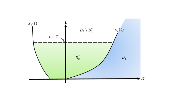
Figure 3.2: The subdomains $D_{1}$, $D_{2}$ and $D_{2}^{T}$.

Let us see that for any fixed $\overline{t}>0$ and $0<T\leq\overline{t}$, the $\mathcal{C}^{1}$ norm of the solution over the domain

$$D_{2}^{T}=\{\left(x,t\right)\colon 0\leq t\leq T,\ x_{1}\left(t\right)\leq x\leq x_{2}\left(t\right)\}$$ (3.69)

is bounded independently of $T$, namely, $\|\left(W_{1},W_{2}\right)\|_{\mathcal{C}^{1}\left(D_{2}^{T}\right)}\leq C\left(\overline{t}\right)$, where
$C\left(\overline{t}\right)>0$ is independent of $0<T\leq\overline{t}$. For a scheme of the situation see figure 3.2. This will be done in two steps. First we will check the boundedness in $\mathcal{C}^{0}$ norm. Afterwards, we will see the boundedness of the derivative (the spatial derivative).

Let $\left(x,t\right)\in D_{2}^{T}$. In order to check the boundedness in $\mathcal{C}^{0}$ norm, we will study the behaviour of the solution and its derivative along the forward and backward characteristics passing through this point. Using H2, any forward characteristic (it will have slope $\lambda_{1}>0$) passing through $\left(x,t\right)$ must intersect the boundary $x_{1}$ at one (only one) point: let this point be $\left(\xi\left(x,t\right),\omega\left(x,t\right)\right)$. Analogously, due to the hiperbolicity, any backward characteristic (slope $\lambda_{2}<0$) must intersect the characteristic curve $x_{2}$ at one (only one) point: let this point be $\left(\eta\left(x,t\right),\beta\left(x,t\right)\right)$. Denote by $W_{2}^{2}\left(t\right)$ the value of $W_{2}$ along the characteristic boundary $x_{2}$. Then

$$W_{2}\left(x,t\right) =W_{2}^{2}\left(\beta\left(x,t\right)\right),$$ (3.70)

$$W_{1}\left(x,t\right) =g\left(W_{2}\left(\xi\left(x,t\right),\omega\left(x,t\right)\right),\omega\left(x,t\right)\right).$$ (3.71)

Since $\beta\left(x,t\right)\leq t$ we have

$$\|W_{2}\|_{\mathcal{C}^{0}\left(D_{2}^{T}\right)}\leq C\left(\overline{t}\right),\;\forall\left(x,t\right)\in D_{2}^{T}\quad\textrm{with }0<T<\overline{t}.$$ (3.72)

Now, since $\omega\left(x,t\right)\leq t$, equations (3.71) and estimation (3.72) imply

$$\|W_{1}\|_{\mathcal{C}^{0}\left(D_{2}^{T}\right)}\leq C\left(\overline{t}\right),\;\forall\left(x,t\right)\in D_{2}^{T}\quad\textrm{with }0<T<\overline{t}.$$ (3.73)

So we have achieved a uniform $\mathcal{C}^{0}$ estimate of the solution.

Let us focus now on its derivatives, starting with the estimation of $\partial W_{2}/\partial x$. When this is done, we repeat the process with $\partial W_{1}/\partial x$ (although a different strategy will be needed). Let

$$v=e^{k\left(W_{1},W_{2}\right)}\frac{\partial W_{2}}{\partial x}$$ (3.74)

where $k$ is defined by means of

$$\frac{\partial k}{\partial W_{1}}=-\frac{1}{\lambda_{1}-\lambda_{2}}\frac{\partial\lambda_{2}}{\partial W_{1}}.$$ (3.75)

It is straight-forward to check that the following ordinary differential equation is satisfied by $v$ along the backward characteristic $x^{\prime}\left(t\right)=\lambda$ where $W_{2}$ is constant:

$$\frac{\partial v}{\partial t}+\lambda_{2}\left(W_{1},W_{2}\right)\frac{\partial v}{\partial x}=-e^{k\left(W_{1},W_{2}\right)}\frac{\partial\lambda_{2}}{\partial W_{2}}v^{2}$$ (3.76)

whose initial condition will be given on $x_{2}\left(t\right)=\lambda_{1}\left(W_{1}^{0},W_{2}^{2}\right)$. In order to see what form has it we note that, on $x_{2}$, we have that

$$\left(W_{2}^{2}\right)^{\prime}\left(t\right)=\frac{\partial W_{2}}{\partial t}+\lambda_{1}\frac{\partial W_{2}}{\partial x}.$$ (3.77)

Since

$$\frac{\partial W_{2}}{\partial t}=-\lambda_{2}\frac{\partial W_{2}}{\partial x}\implies\frac{\partial W_{2}}{\partial x}=\frac{\left(W_{2}^{2}\right)^{\prime}\left(t\right)}{\lambda_{1}-\lambda_{2}}$$ (3.78)

on $x_{2}$. Therefor, the initial condition can be written as

$$v|_{x_{2}}=\frac{e^{k\left(W_{1}^{0},W_{2}^{2}\right)}}{\left(\lambda_{1}\left(W_{1}^{0},W_{2}^{2}\right)-\lambda_{2}\left(W_{1}^{0},W_{2}^{2}\right)\right)}\left(W_{2}^{2}\right)^{\prime}\left(t\right).$$ (3.79)

The initial-value problem (3.76) and (3.79) has a solution $v$ which is given by

$$v\left(x,t\right)=\frac{e^{k\left(W_{1}^{0},W_{2}^{2}\left(\beta\right)\right)}\left(W_{2}^{2}\right)^{\prime}\left(\beta\right)}{B\left(\beta\left(x,t\right),t\right)}$$ (3.80)

where

$$B\left(\beta,t\right)= \lambda_{1}\left(W_{1}^{0},W_{2}^{2}\left(\beta\right)\right)-\lambda_{2}\left(W_{1}^{0},W_{2}^{2}\left(\beta\right)\right)$$ (3.81)

$$+\left(W_{2}^{2}\right)^{\prime}\left(\beta\right)e^{k\left(W_{1}^{0},W_{2}^{2}\left(\beta\right)\right)}$$ (3.82)

$$\times\int_{\beta}^{t}\left[\frac{\partial\lambda_{2}}{\partial W_{2}}\left(W_{1}\left(\widetilde{x}\left(\beta,\tau\right),\tau\right),W_{2}^{2}\left(\beta\right)\right)e^{k\left(W_{1}\left(\widetilde{x}\left(\beta,\tau\right),\tau\right),W_{2}^{2}\left(\beta\right)\right)}\right]\mathrm{d}\tau.$$ (3.83)

Here, $x=\widetilde{x}\left(\beta,\tau\right)$ denotes the backward characteristic passing through the point $\left(\eta,\beta\right)$. Using hypothesis H2 we have that $\lambda_{1}-\lambda_{2}$ is bounded uniformly away from zero, and using hypotheses H3 and H5 we have that $\left(W_{2}^{2}\right)^{\prime}\partial\lambda_{2}/\partial W_{2}\geq 0$. With this, we conclude that $B$ is non-zero and hence we have arrived to a uniform bound of $v$, that is, a uniform bound of $\partial W_{2}/\partial x$:

$$\left|\frac{\partial W_{2}}{\partial x}\left(x,t\right)\right|\leq C\left(\overline{t}\right),\quad\forall\left(x,t\right)\in D_{2}^{T},\quad 0<T\leq\overline{t}.$$ (3.84)

Furthermore, we get that the sign of $\partial W_{2}/\partial x$ is the same that $\left(W_{2}^{2}\right)^{\prime}\left(t\right)$ which is negative.

Finally, we estimate $\partial W_{1}/\partial x$, in turn, in three steps:

1. Let us see the sign of $\partial W_{1}/\partial x$ on $x=x_{1}\left(t\right)$. Differentiating $W_{1}=g\left(W_{2},t\right)$ along $x=x_{1}\left(t\right)$ we have

   $$\frac{\partial W_{1}}{\partial x}=\frac{1}{x_{1}^{\prime}\left(t\right)-\lambda_{1}}\left[\frac{\partial g}{\partial W_{2}}\cdot\left(x_{1}^{\prime}\left(t\right)-\lambda_{2}\right)\cdot\frac{\partial W_{2}}{\partial x}\right].$$ (3.85)

   Now, since

   • $\lambda_{2}<x_{1}^{\prime}\left(t\right)<\lambda_{1}$ by H2;

   • $\partial W_{2}/\partial x<0$ as we said previously;

   • $\partial g/\partial W_{2}\geq 0$ by H4;

   • $\partial g/\partial t\leq 0$ by assumption

   we obtain that

   $$\frac{\partial W_{1}}{\partial x}=\underbrace{\frac{1}{x_{1}^{\prime}\left(t\right)-\lambda_{1}}}_{<0}\left[\underbrace{\frac{\partial g}{\partial W_{2}}}_{\geq 0}\cdot\left(\underbrace{x_{1}^{\prime}\left(t\right)-\lambda_{2}}_{>0}\right)\cdot\underbrace{\frac{\partial W_{2}}{\partial x}}_{<0}\right].$$ (3.86)

   and hence $\partial W_{1}/\partial x\geq 0$ on $x_{1}\left(t\right)$.

2. Now we check the sign of $\partial W_{1}/\partial x$ but now in $D_{2}^{T}$. Since $W_{1}$ is constant along the forward characteristic (is a Riemann invariant) we have

   $$W_{1}\left(x,t\right)=W_{1}\left(\xi\left(x,t\right),\omega\left(x,t\right)\right),\quad\forall\left(x,t\right)\in D_{2}^{T}$$ (3.87)

   where $\xi\left(x,t\right)=x_{1}\left(\omega\left(x,t\right)\right)$. Therefor,

   $$\frac{\partial W_{1}}{\partial x}\left(x,t\right) =\frac{\partial W_{1}}{\partial t}\left(\xi,\omega\right)\frac{\partial\omega}{\partial x}\left(x,t\right)+\frac{\partial W_{1}}{\partial x}\left(\xi,\omega\right)\frac{\partial\xi}{\partial x}\left(x,t\right)$$ (3.88)

   $$=\left(x_{1}^{\prime}\left(t\right)-\lambda_{1}\right)\frac{\partial W_{1}}{\partial x}\left(\xi,\omega\right)\frac{\partial\omega}{\partial x}\left(x,t\right).$$ (3.89)

   To determine the sign of $\partial W_{1}/\partial x$ in $D_{2}^{T}$ we first notice that $x_{1}^{\prime}-\lambda_{1}<0$ and $\partial W_{1}/\partial x\left(\xi,\omega\right)\geq 0$. From the definition of $\omega$, we see that it decreases as $x$ increases, so $\partial\omega/\partial x\leq 0$. With this, we conclude that $\partial W_{1}/\partial x\geq 0$ in $D_{2}^{T}$.

3. Finally, let us see the $\mathcal{C}^{0}$-estimate of $\partial W_{1}/\partial x$ in $D_{2}^{T}$. Let

   $$u=e^{h\left(W_{2},W_{1}\right)}\frac{\partial W_{2}}{\partial x}$$ (3.90)

   where

   $$\frac{\partial h}{\partial W_{2}}=\frac{1}{\lambda_{1}-\lambda_{2}}\frac{\partial\lambda_{1}}{\partial W_{2}}.$$ (3.91)

   This function $u$ satisfies the ODE

   $$\frac{\partial u}{\partial t}=-e^{-h\left(W_{2},W_{1}\right)}\frac{\partial\lambda_{1}}{\partial W_{1}}u^{2}$$ (3.92)

   along the characteristic $x^{\prime}=\lambda_{1}$. The initial condition is given on
   $x_{1}\left(t\right)=\left(\xi\left(x,t\right),\omega\left(x,t\right)\right)$ and has the form

   $$u\left(\xi,\omega\right)=e^{h\left(W_{1}\left(\xi,\omega\right),W_{2}\left(\xi,\omega\right)\right)}\frac{\partial W_{1}}{\partial x}\left(\xi,\omega\right).$$ (3.93)

   By integration we get

   $$u\left(x,t\right)=\frac{e^{h\left(W_{1}\left(\xi,\omega\right),W_{2}\left(\xi,\omega\right)\right)}}{A\left(\omega,t\right)}\frac{\partial W_{1}}{\partial x}\left(\xi,\omega\right)$$ (3.94)

   with

   $$\begin{split}A\left(\omega,t\right)&=1+\frac{\partial W_{1}}{\partial x}\left(\xi,\omega\right)e^{h\left(W_{1}\left(\xi,\omega\right),W_{2}\left(\xi,\omega\right)\right)}\\ &\times\int_{\omega}^{t}\frac{\partial\lambda_{1}}{\partial W_{1}}\left(W_{1}\left(\widetilde{x}\left(\omega,\tau\right),\tau\right),W_{2}\left(\xi,\omega\right)\right)e^{-h\left(W_{1}\left(\widetilde{x}\left(\omega,\tau\right),\tau\right),W_{2}\left(\xi,\omega\right)\right)}\mathrm{d}\tau\end{split}$$ (3.95)

   where $x=\widetilde{x}\left(\omega,\tau\right)$ is the forward characteristic passing through the point $\left(\xi,\omega\right)$. Now, due to hypothesis H5 we have that $\partial\lambda_{1}/\partial W_{1}\geq 0$ and due to Step 1 we have that $\partial W_{1}/\partial x\geq 0$ on $x_{1}\left(t\right)$ so, we see that $A\left(\omega,t\right)$ is never zero. With this, using hypothesis H2 and the uniform estimates of $W_{2},W_{1}$ and $\partial W_{2}/\partial x$ in $D_{2}^{T}$ we get the uniform estimate for $\partial W_{1}/\partial x$ on $D_{2}^{T}$.

   Concluding, since this estimate is independent of $T$ and $D=D_{1}\cup D_{2}$ we complete the proof.

∎

Let us check if these hypotheses are satisfied for our problem. Writing all together we have:

$$W_{1,2} =u\pm 4\sqrt{\frac{\beta}{2\rho}}A^{1/4},$$ (3.96)

$$A =\left(\frac{W_{1}-W_{2}}{4}\right)^{4}\left(\frac{\rho}{2\beta}\right)^{2},$$ (3.97)

$$u =\frac{W_{1}+W_{2}}{2},$$ (3.98)

$$x_{1}(t) =0\;\forall t,$$ (3.99)

$$W_{2}(x_{1}(t),t) =W_{2}(0,t)=u_{\textrm{inflow}}-4\sqrt{\frac{\beta}{2\rho}}A_{\textrm{inflow}}^{1/4},$$ (3.100)

$$\lambda_{1,2} =u\pm 4\sqrt{\frac{\beta}{2\rho}}A^{1/4},$$ (3.101)

$$W_{1}^{0}(x) =W_{2}^{0}(x)=u_{0}(x)\pm 4\sqrt{\frac{\beta}{2\rho}}A_{0}^{1/4},$$ (3.102)

where $u_{\textrm{inflow}}=u(0,t)$ and $A_{\textrm{inflow}}=A(0,t)$. Now, regarding the hypotheses:

1. We need the initial velocity and the boundary conditions to be $\mathcal{C}^{1}$, which is physically correct (without abrupt accelerations).

2. Since $\lambda_{1}>0$ and $\lambda_{2}<0$ as we said before, this hypothesis is satisfied.

3. The boundedness is achieved due to biological reasons, and we need to choose $u_{0}$ to be constant.

4. Replacing equations (3.97) and (3.98) into the expression of $g$ (3.100), we see that this hypothesis is also satisfied.

But the problem comes with the fifth and sixth hypotheses, that are false in our case. Indeed,

$$\lambda_{2}=W_{2}\implies\frac{\partial\lambda_{2}}{\partial W_{2}}=1>0.$$ (3.103)

Nevertheless, since it is a sufficient condition, we could get smoothness of the solution in this case too. In fact, this is checked via numerical simulations in chapter 5.

With a slightly modification of the equations and other tube law, it is shown in [15] that under some plausible conditions such as the no-singularity of the cross-sectional area and a pulsating boundary conditions (such as heart beats) the thesis of the previous theorem is achieved.

3.2.1 Shock wave formation in compliant arteries

We have just seen that we can not assure smooth solutions. This makes also clinical sense since if the heart beats are too abrupt, for example, the blood could be faster than the usual blood wave: this is precisely the condition for a shock wave to form.

Motivated for this fact, we study when and where the first shock wave could be formed and which factors are relevant to it.

Next we present an original result where we obtain an explicit formulation for when the first shock wave appears. Furthermore, we will see the direct influence of the physical parameters to characterise from clinical data if this pathology happens. We have followed the steps of Čanić and Kim [15], although they used a slight different formulation. Keener and Sneyd also obtained a similar (but less general) result in [61]. This result was presented in $2017$ in the 4º Congreso de jóvenes investigadores (IV Conference for young researchers) (see [101])

Theorem 3.

Assuming constant initial data

$$A(x,0)=A_{0},\qquad u(x,0)=0,$$ (3.104)

the time $t_{s}$ of the first shock formation is given by

$$t_{s}=\omega+\frac{\lambda_{1}}{u_{\textrm{inflow}}^{\prime}(t)}=\omega+\frac{u_{\textrm{inflow}}+4\sqrt{\beta/(2\rho)}A_{\textrm{inflow}}^{1/4}}{u_{\textrm{inflow}}^{\prime}(t)}.$$ (3.105)

where $\omega$ is the first time when the forward characteristic intersects the left spatial boundary.

Proof.

In terms of the Riemann invariants, the initial data read $W_{1}^{0}(x)=W_{2}^{0}(x)=u_{0}(x)\pm 4\sqrt{\frac{\beta}{2\rho}}A_{0}^{1/4}$. For this set of initial data, $W_{1}$ is constant everywhere in the region of smooth flow; the characteristics are straight lines in

$$D_{2}=\{(x,t)\colon x_{2}(t)\leq x<+\infty,\ t\geq 0\},$$ (3.106)

where $x_{2}(t)$ is the forward characteristic $x_{2}^{\prime}=\lambda_{1}$ emanating from $(0,0)$. The solution in region

$$D_{1}=\{(x,t)\colon 0\leq x\leq x_{2}(t),\ t\geq 0\},$$ (3.107)

bounded by the left boundary $x_{1}=0$ and the forward characteristic $x_{2}$, is driven by $u(\cdot,t)$ on $x_{1}$ and will develop shock waves due to the fact that $u^{\prime}(\cdot,t)$ changes sign.

To estimate the time $t_{s}$ we note that at the point $(t_{s},x_{s})$ the partial derivative $\partial W_{1}/\partial x$ blows up, as we can see in figure 3.1(c). This occurs at the point where the denominator $A(\omega,t)$ in (3.94) becomes equal to zero. We recall that its expression was

$$\begin{split}A\left(\omega,t\right)&=1+\frac{\partial W_{1}}{\partial x}\left(\xi,\omega\right)e^{h\left(W_{1}\left(\xi,\omega\right),W_{2}\left(\xi,\omega\right)\right)}\\ &\times\int_{\omega}^{t}\frac{\partial\lambda_{1}}{\partial W_{1}}\left(W_{1}\left(\widetilde{x}\left(\omega,\tau\right),\tau\right),W_{2}\left(\xi,\omega\right)\right)e^{-h\left(W_{1}\left(\widetilde{x}\left(\omega,\tau\right),\tau\right),W_{2}\left(\xi,\omega\right)\right)}\mathrm{d}\tau.\end{split}$$ (3.108)

Hence, it can be calculated by recalling that $\lambda_{1}=W_{1}$, what means that $\partial\lambda_{1}/\partial W_{1}=1$ and that $W_{1}=W_{1}^{0}$ everywhere. This implies that in (3.108)

$$e^{h\left(W_{1}\left(\xi,\omega\right),W_{2}\left(\xi,\omega\right)\right)-h\left(W_{1}\left(\widetilde{x}\left(\omega,\tau\right),\tau\right),W_{2}\left(\xi,\omega\right)\right)}=1$$ (3.109)

and so

$$A(\omega,t)=1+\frac{\partial W_{1}}{\partial x}(\xi,\omega)(t-\omega).$$ (3.110)

From equation (3.85) we see that

$$\left.\frac{\partial W_{1}}{\partial x}\right|_{x_{1}=0}=-2\frac{u^{\prime}(t)}{\lambda_{1}}+\frac{\lambda_{1}}{\lambda_{2}}\frac{\partial W_{2}}{\partial x}.$$ (3.111)

Since $\partial W_{2}/\partial x=0$, we obtain

$$A(\omega,t)=1-\frac{u^{\prime}(t)}{\lambda_{1}}(t-\omega).$$ (3.112)

Therefor, isolating, the first time the shock forms is equal to

$$t_{s}=\omega+\frac{\lambda_{1}}{u_{\textrm{inflow}}^{\prime}(t)}=\omega+\frac{u_{\textrm{inflow}}+4\sqrt{\beta/(2\rho)}A_{\textrm{inflow}}^{1/4}}{u_{\textrm{inflow}}^{\prime}(t)}.$$ (3.113)

∎

Two remarkable conclusions become deduced from this result: the shock will be produced earlier if the inflow accelerates and if the walls of the vessel are less rigid (due to the $\beta$ factor).

A case that could be interesting from a medical point of view is to see, in the case of the aorta since is the one where we can find more literature, if this model can explain the pistol-shot heard in aortic insufficiency. Taking as an approximation the measures done in [34, 80, 24] we assume $A_{0}=A_{\textrm{inflow}}\approx 4\times 10^{-2}m$. Regarding blood flow velocity we have assumed $1$ m/s, following the measures found in [82]. Recalling that

$$\beta=\frac{\sqrt{\pi}Eh}{(1-\nu^{2})A_{0}},$$ (3.114)

we will use the parameters of appendix A.

Now, for a healthy human being we have taken $u_{\textrm{inflow}}^{\prime}=7$m/s², following the correlations of [82] and a Young’s modulus of $E=10^{5}\ Pa$. Hence, the value for the first time and place when shock forms is

$$t_{s}\approx\frac{1+4\sqrt{29633.5/(2\times 1050)}(4\times 10^{-2})^{1/4}}{7}\approx 1.1\text{s}$$ (3.115)

and

$$x_{s}=t_{s}\lambda_{1}\approx 8.5\textrm{m},$$ (3.116)

which, according to [31] is far from the mean length value of the aorta, $33.2$ cm.

Now, for a sick human being, say by aortic insufficiency, the heart increases its volume and since the aortic valve does not close properly, the muscle must do a greater contraction, so a greater blood flow acceleration happens in each heart beat (see [50]). Using the same bibliography as we have previously consulted, we could have that $u_{\textrm{inflow}}^{\prime}=15$ m/s². Moreover, the arteries could be not rigid enough (what may cause an aneurysm), say $E=2\cdot 10^{3}Pa$. With this variation we would have:

$$t_{s}\approx\frac{1+4\sqrt{592.67/(2\times 1050)}(4\times 10^{-2})^{1/4}}{15}\approx 0.13\text{s}$$ (3.117)

and

$$x_{s}=t_{s}\lambda_{1}\approx 0.25\textrm{m}.$$ (3.118)

As it should be, this case is worse for the patient and a shock wave is formed inside the typical length of the aorta. For the interested reader, some research has been done in this line, although with different and sometimes less general models. See [33, 84, 105]. Henceforth, we move on to the numerical simulations. Although shock waves have not been simulated due to complexity of controlling the inflow data, healthy cases have been simulated. For these simulations the method used has been the Galerkin Discontinuous Finite Element Method, presented in the next chapter.

Chapter 4 Discontinuous Galerkin Method

In computational fluid dynamics, specially in medical applications, accuracy is preferred rather than velocity or simplicity in numerical methods. We must require a number of key properties such as flexibility in geometry, robustness, efficiency, high-order or variable order accuracy — since long time integration is needed — and, if possible, possibility of high performance computing.

During the last decades, a number of numerical techniques for the solution of nonlinear conservation laws, nonlinear convection-diffusion problems and compressible flow have been developed. We first review briefly the three most popular: finite differences, finite volumes and finite elements.

• Finite-difference methods (FDM) are discretisation methods for solving differential equations by approximating them with difference equations, in which finite differences approximate the derivatives. This is usually done using Taylor series expansion and truncating at the desired order. Due to this, we can achieve any order desired for the method, which is an advantage.

  The two sources of error in finite difference methods are round-off error — loss of precision due to computer machine — and discretisation error, the difference between the exact solution and the exact approximation assuming perfect arithmetic (that is, assuming no round-off).

  This method relies on discretising a function on a grid, so to approximate the solution to a problem, one must first discretise the problem’s domain. This is usually done by dividing the domain into a uniform grid. Therefor, the solution is recovered in a pointwise way. It can be shown that the truncation error is proportional to the step sizes (time and space steps). If we reduce the step size or increase the truncation of the Taylor’s expansion the accuracy of the approximate solution increases, but also the simulation’s duration. Therefor, a reasonable balance between data quality and simulation duration is necessary for practical usage. Large time steps are useful for increasing simulation speed in practice. However, time steps which are too large may create instabilities and affect the data quality [54, 79]. There are quite a lot of variations of the FDM, both explicit and implicit cases and quite a lot of theory behind these methods, since FDMs are the dominant approach to numerical solutions of partial differential equations [49]. For a first approach to these methods we refer the interested reader to [58, 5, 6]. The main drawback of these methods is that complex geometries are not allowed in a simple way.

• Similar to the FDM, in the finite volume method (FVM), values are calculated at discrete places on a meshed geometry [76, 118, 65]. “Finite volume” refers to the small volume surrounding each node point on a mesh (control volumes, or cells). In the finite volume method, volume integrals in a partial differential equation that contain a divergence term are converted to surface integrals, using the divergence theorem. These terms are then evaluated as fluxes at the surfaces of each finite volume. Thus, FVMs use piecewise constant approximations. Because the flux entering a given volume is identical to that leaving the adjacent volume, these methods are conservative. Another advantage of the finite volume method is that it is easily formulated to allow for unstructured meshes and, since it uses cell averages, it allows discontinuities. The problem comes when we want to achieve high order on general grids. Also, there are requirements of grid smoothness non trivial at all [47, 10, 51]. For a survey of various techniques and results from the FVM, we refer the reader to the monograph [36].

• The next step is the family of finite element methods (FEM). It is also referred to as finite element analysis (FEA). The main basic steps of the FEM are [78]:

  1. Divide the whole domain of the problem into subdomains (can be a regular or unstructured mesh) called finite elements.

  2. Convert the differential equations we are dealing with into its weak form, multiplying by an arbitrary function and integrating.

  3. Choose appropriate test functions (they are usually polynomials) to arrive to an algebraic system, and solve it.

  Regarding the history, as it is often the case with original developments, it is rather difficult to quote an exact date of invention, but in [12], the roots of the FEM are traced back to three separate research groups: applied mathematicians [22], physicists [116] and engineers [52], although the FEM obtained its real impetus from the development of engineers. These methods can achieve high order and can deal without many problems complex geometries. The main issue is that they are implicit in time and when we are dealing problems with direction (such a diffusion) are not really well suited.

To sum up the observations, we have:

	Complex geometries	High-order accuracy	Explicit semi-discrete form
FDM	$\times$	✓	✓
FVM	✓	$\times$	✓
FEM	✓	✓	$\times$

Table 4.1: Advantages and disadvantages of the most used methods for solving differential equations numerically.

The ideal case would be to have a scheme with local high-order and flexible elements as in the FEM; the nice handling of discontinuities as in the FVM; and the explicit and relatively simple (semi-)discrete form of the FDM. We can find indeed a method with these components, inside the FEMs, called Discontinuous Galerkin Finite Element Method (DG-FEM, DGM or simply DG).

As happened with FEM, DG methods can be considered as numerical schemes for the weak formulation of the equations. They were first applied to first-order equations by Reed and Hill in [98], but their widespread use followed from the application to hyperbolic problems by Cockburn and collaborators in a series of articles [20, 19, 21]. In the DG-FEM framework, the solution is recovered in a more continuous way, with polynomials, without the need of using a reconstruction operator (such as interpolation). This feature of DG schemes is in common with the classical FEM. But, unlike classical finite elements, the numerical solution given by a DG scheme is discontinuous at element interfaces and this discontinuity is resolved by the use of a so-called numerical flux function, which is a common feature with FVM.

Hence, in the next sections we will give more details about this method, starting from definitions and some mathematical notation up to the computational implementation. As we said in the previous chapters, we are treating with a one-dimensional problem, so both the theory as the implementation are a little simpler. For a more general theoretical treatment (dimensions $2$ and $3$) we refer the interested reader to the lecture notes [30].

4.1 Notation

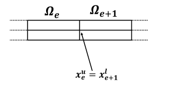
Figure 4.1: One dimensional finite element discretisation.

The idea of this family of methods is to split the domain we are dealing with, namely $\Omega=[a,b]$, into a set of the so-called elements, in our case they are subintervals as shown in figure 4.1. Formally we have

$$\Omega=\bigcup_{e=1}^{N_{\textrm{el}}}\Omega_{e},$$ (4.1)

$$\Omega_{e}=[x^{u}_{e},x^{l}_{e}]$$ (4.2)

where

$$x_{e}^{u}=x_{e+1}^{l}.$$ (4.3)

This subdivision of the general domain $\Omega$ will be denoted by $\mathcal{T}_{h}$ and we call it the triangulation of $\Omega$ (for analogy to the two and three-dimensional cases).

By $\mathcal{F}_{h}$ we denote the set of boundaries of the elements, namely

$$\mathcal{F}_{h}=\left\{x_{e}^{l}\right\}_{e=1}^{N_{\textrm{el}}}\cup\left\{x_{N_{\textrm{el}}}^{u}\right\}=\left\{x_{e}^{u}\right\}_{e=1}^{N_{e}l}\cup\left\{x_{1}^{l}\right\}.$$ (4.4)

Moreover, we will sometimes treat in a separated way the inlet and outlet boundaries, so

$$\mathcal{F}_{h}^{io}=\left\{x_{1}^{l}\right\}\cup\left\{x_{N_{\textrm{el}}}^{u}\right\},$$ (4.5)

$$\mathcal{F}_{h}^{W}=\mathcal{F}_{h}\setminus\mathcal{F}_{h}^{io}.$$ (4.6)

First we recall some standard notation from the measure and integral Lebesgue theory.

4.1.1 Measure and integral Lebesgue notation

Let $M\subset\mathbb{R}^{n}$, $n=1,2,\dots$ be a Lebesgue measurable set. We recall that two measurable functions are equivalent if they differ at most on a set of zero Lebesgue measure. The Lebesgue space $L^{p}(M)$, with $1\leq p<\infty$ is the linear space of all functions measurable on $M$ (more precisely, of classes of equivalent measurable functions) such that

$$\int_{M}|u|^{p}\mathrm{d}x<+\infty.$$ (4.7)

With this, let $k\geq 0$ be an artbitrary integer and $1\leq p<\infty$. We define the Sobolev space $W^{k,p}(M)$ as the space of all functions from the space $L^{p}(M)$ whose distributional derivatives $D^{\alpha}u$, up to order $k$, also belong to $L^{p}(M)$, i.e.,

$$W^{k,p}(M)=\{u\in L^{p}(M)\colon D^{\alpha}u\in L^{p}(M)\,\forall\alpha,\ |\alpha|\leq k\}.$$ (4.8)

For $p=2$, $W^{k,2}$ is a Hilbert space and we denote it by $H^{k}(M)$. Now, the DGM is based on the use of discontinuous approximations. This is the reason why over a triangulation $\mathcal{T}_{h}$, we define the broken Sobolev space

$$H^{k}(\Omega,\mathcal{T}_{h})=\{u\in L^{2}(\Omega)\colon u|_{\Omega_{e}}\in H^{k}(\Omega_{e})\,\forall\Omega_{e}\in\mathcal{T}_{h}\}.$$ (4.9)

Since we will be working with two dimensional vector-valued functions we will denote

$$\textbf{H}^{k}(\Omega,\mathcal{T}_{h})=H^{k}(\Omega,\mathcal{T}_{h})\times H^{k}(\Omega,\mathcal{T}_{h}).$$ (4.10)

The DGM can be characterised as a finite element technique using piecewise polynomial approximations, in general discontinuous on interfaces between neighbouring elements. Therefor, we introduce a finite-dimensional subspace of $H^{k}(\Omega,\mathcal{T}_{h})$, where the approximate solution will be sought.

Let $\mathcal{T}_{h}$ be a triangulation of $\Omega$ and let $p\geq 0$ be an integer. We define the space of discontinuous piecewise polynomial functions

$$S_{hP}=\{v\in L^{2}(\Omega)\colon v|_{\Omega_{e}}\in\mathcal{P}_{P}(\Omega_{e})\,\forall\Omega_{e}\in\mathcal{T}_{h}\},$$ (4.11)

where $\mathcal{P}_{P}(\Omega_{e})$ denotes the space of all polynomials of degree $\leq P$ on $\Omega_{e}$. Obviously, $S_{hP}\subset H^{k}(\Omega,\mathcal{T}_{h})$ for any $k\geq 1$ and its dimension is $\dim S_{hP}=P+1$.

Similarly as we have done before, we will denote

$$\textbf{S}_{hP}=S_{hP}\times S_{hP}.$$ (4.12)

Finally, since we are going to deal with vectorial functions, we will understand operations such as integration of derivation of the vector as the operation component-wise.

4.2 DG space (semi)discretisation

In order to give a more general situation, this time we will consider the source term, namely the friction term. Since we are assuming that the blood is a Newtonian fluid, the friction term has the form

$$f=-K_{R}u,$$ (4.13)

where $K_{R}$ is a strictly positive quantity which represents the viscous resistance of flow per unit length of tube. We still assume that $\alpha=1$ (a flat profile) for the reasons we discussed in subsection 3.1.2. Hence, we can write the system as

$$\textbf{U}_{t}+\textbf{F}_{x}=\textbf{T}$$ (4.14)

with

$$\textbf{U}=\begin{bmatrix}A\\ u\end{bmatrix},\quad\textbf{F}=\begin{bmatrix}uA\\ \frac{u^{2}}{2}+\frac{p}{\rho}\end{bmatrix}\quad\text{and}\quad\text{{T}}=\begin{bmatrix}0\\ \frac{K_{R}}{\rho}u\end{bmatrix}.$$ (4.15)

In order to derive the discrete problem, we assume that there exists an exact solution $\textbf{U}\in\mathcal{C}^{1}(\textbf{H}^{1}(\Omega,\mathcal{T}_{h});[0,T])$, where $T>0$ represents the final time, of the Navier-Stokes equations (4.14). Then we multiply (4.14) by a test function $\boldsymbol{\psi}\in\textbf{H}^{1}(\Omega,\mathcal{T}_{h})$ and integrate over the domain. Specifying the dependency on U we obtain:

$$\int_{\Omega}\textbf{U}_{t}\boldsymbol{\psi}\mathrm{d}x+\int_{\Omega}\textbf{F}_{x}(\textbf{U})\boldsymbol{\psi}\mathrm{d}x=\int_{\Omega}\textbf{T}(\textbf{U})\boldsymbol{\psi}.$$ (4.16)

Let us denote, for a measurable set $M$, the inner product of $L^{2}(M)$ with

$$\int_{M}uv\mathrm{d}x=\left\langle u,v\right\rangle_{M}.$$ (4.17)

At this point is where the main difference with respect to the FEM appears. We do not demand continuity between elements, and since the elements of the triangulation $\mathcal{T}_{h}$ are disjoint, we can decouple (4.16) and work separately with each $\Omega_{e}\in\mathcal{T}_{h}$ as:

$$\left\langle\textbf{U}_{t},\boldsymbol{\psi}\right\rangle_{\Omega_{e}}+\left\langle\textbf{F}_{x}(\textbf{U}),\boldsymbol{\psi}\right\rangle_{\Omega_{e}}=\left\langle\textbf{T}(\textbf{U}),\boldsymbol{\psi}\right\rangle_{\Omega_{e}}.$$ (4.18)

We integrate by parts the flux term (in higher dimensions this would be equivalent to apply Green’s theorem):

$$\left\langle\textbf{U}_{t},\boldsymbol{\psi}\right\rangle_{\Omega_{e}}+\left[\textbf{F}(\textbf{U})\cdot\boldsymbol{\psi}\right]_{x_{e}^{l}}^{x_{e}^{u}}-\left\langle\textbf{F}(\textbf{U}),\boldsymbol{\psi}_{x}\right\rangle_{\Omega_{e}}=\left\langle\textbf{T}(\textbf{U}),\boldsymbol{\psi}\right\rangle_{\Omega_{e}}.$$ (4.19)

We remark that the term evaluated in the boundary is interpreted as component-wise. It is not the usual dot product of vectors.

As we said before, we discretise the solution U with an approximation $\textbf{U}_{h}\in\textbf{S}_{hP}$. Due to the fact that $\dim S_{hP}=P+1$, we can express this discrete solution as a linear combination

$$\left.\textbf{U}_{h}\right|_{\Omega_{e}}=\sum_{p=0}^{P}\hat{\textbf{U}}_{p}^{e}\varphi_{p}$$ (4.20)

where $\{\varphi_{p}\}_{p=0}^{P}$ is a basis of the space $S_{hP}$. In the previous expression, the product denotes a component-wise product.

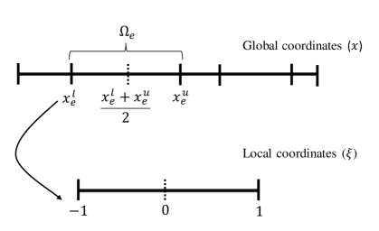
Figure 4.2: Change of coordinates from global to local at an element.

Now, this expansion is carried out at each element $\Omega_{e}\in\mathcal{T}_{h}$, so we need to do a readjustment of the coordinates. More precisely, the global semidiscrete solution $\textbf{U}_{h}$ is defined in all the length of the artery, namely $0\leq x\leq l$. But at each element we need to resize to $-1\leq\xi\leq 1$, see figure 4.2. To carry out this conversion, affine mappings (common in FEM) are used. Their expression, from global to local and local to global coordinates are, respectively,

$$\xi(x_{e}) =\frac{2x-x_{e}^{l}-x_{e}^{u}}{x_{e}^{u}-x_{e}^{l}},$$ (4.21)

$$x_{e}(\xi) =x_{e}^{l}\frac{1-\xi}{2}+x_{e}^{u}\frac{1+\xi}{2},$$ (4.22)

(obviously one mapping is the inverse function of the other one). More precisely equation (4.20) has the form

$$\left.\textbf{U}_{h}(x_{e},t)\right|_{\Omega_{e}}=\sum_{p=0}^{P}\hat{\textbf{U}}_{p}^{e}(t)\varphi_{p}(\xi).$$ (4.23)

We remark that the coefficients of the previous expressions only depend on time. This is the characteristic of the so-called modal form of a finite element method. The other possibility is the nodal form, where the solution is calculated in some points (nodes) of each element. These coefficients are usually called degrees of freedom. Here is where the main distinctive of the Galerkin methods come out: the test function $\boldsymbol{\psi}$ also belongs to the finite-dimensional space $\textbf{S}_{hP}$, indeed it will be the same on each component, so we will change the notation to $\psi$. With this, the first term of (4.19) is approximated by

$$\left\langle\textbf{U}_{t}(x_{e}(\xi),t),\psi(\xi)\right\rangle_{I}=\left\langle\frac{\partial\textbf{U}(x_{e}(\xi),t)}{\partial t},\psi(\xi)\right\rangle_{I}\approx\sum_{p=0}^{P}\frac{\partial\hat{\textbf{U}}_{p}^{e}(x_{e}(\xi),t)}{\partial t}\left\langle\varphi_{p}(\xi),\psi(\xi)\right\rangle_{I},$$ (4.24)

where $I=[-1,1]$. Moreover, by substitution of variables, the third term of equation (4.19) becomes

$$\begin{split}\left\langle\textbf{F}(\textbf{U}),\boldsymbol{\psi}_{x}\right\rangle_{\Omega_{e}}=&\int_{\Omega_{e}}\textbf{F}(\textbf{U}(x,t))\psi_{x}(\xi(x_{e}))\ \mathrm{d}x\\ =\frac{2}{x_{e}^{u}-x_{e}^{l}}&\int_{-1}^{1}\textbf{F}(\textbf{U}(\xi,t))\psi_{x}(\xi)\ \mathrm{d}\xi=\frac{2}{x_{e}^{u}-x_{e}^{l}}\left\langle\textbf{F}(\textbf{U}),\psi_{x}\right\rangle_{I}.\end{split}$$ (4.25)

Up to now there are some unclear points in the reasoning previously done. First of all, the election of the test and basis functions. In the next subsection we will choose them motivating the election.

4.2.1 Election of test and basis functions

In a benchmark more common in calculus, test functions are chosen as $\mathcal{C}^{\infty}$ with compact support. Nevertheless, for practical uses we consider both the test function $\psi$ and the basis functions $\{\varphi_{p}\}_{p}$ belonging to the piecewise polynomial space $S_{hP}$. More precisely, in order to avoid the appearance of more coefficients we choose the test functions as one of the basis functions. The idea of this is that in the expression

$$\sum_{p=0}^{P}\frac{\partial\hat{\textbf{U}}^{e}_{p}(x_{e}(\xi),t)}{\partial t}\left\langle\varphi_{p}(\xi),\varphi_{q}(\xi)\right\rangle_{I}$$ (4.26)

by varying the test function all over the basis functions, we decouple the system, so we can isolate the derivative of the degrees of freedom. The previous equation can be seen as a product matrix-vector

$$\mathcal{M}\hat{\textbf{U}}^{e}$$ (4.27)

where

$$\mathcal{M}_{ij}=\left\langle\varphi_{i},\varphi_{j}\right\rangle_{I},\qquad\hat{\textbf{U}}^{e}=\begin{bmatrix}\hat{\textbf{U}}_{1}^{e}\\ \vdots\\ \hat{\textbf{U}}_{P}^{e}\end{bmatrix}.$$ (4.28)

The most straightforward election would be to choose the canonical basis

$$\varphi_{p}(\xi)=\xi^{p-1}.$$ (4.29)

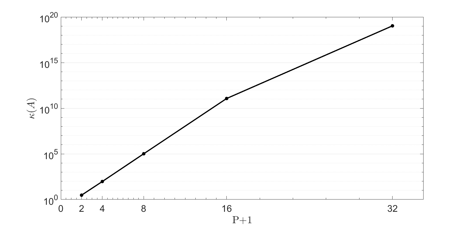
Figure 4.3: Condition number (in norm $1$) of the matrix $\mathcal{M}$. As we can see, it grows almost exponentially.

As a quality measure, we can look to the condition number of $\mathcal{M}$. In the norm $1$, for example, we can see that it grows very quickly, as we present in figure 4.3. Therefor, this election does not look like a robust choice for high $P$.

With this understanding, we look for a better basis, specifically one which makes $\mathcal{M}$ diagonal. I.e., we want an orthogonal basis. The basis usually chosen is the one formed by Legendre’s polynomials. Instead of enumerating the properties, in this subsection we will reason in a straightforward manner its appearance. Some useful properties of these polynomials are proved using basic algebra and calculus.

First of all, we apply the Gram-Schmidt process to the canonical basis and we get a complete orthogonal basis $\{Q_{n}\}_{n=0}^{P}$, where $Q_{0}(x)=1$ and

$$Q_{n}(x)=x^{n}-\sum_{i=0}^{n-1}\frac{\left\langle x^{n},Q_{i}\right\rangle_{I}}{\left\langle Q_{i},Q_{i}\right\rangle_{I}}Q_{i}(x).$$ (4.30)

Now we need a result about orthogonal bases extracted from [66]:

Proposition 4.

Let $\{p_{n}\}_{n=0}^{\infty}$ be an orthogonal polynomial sequence (OPS) in $L^{2}([a,b])$ with $\deg(p_{n})=n$. Then

1. $\left\langle x^{k},p_{n}\right\rangle_{[a,b]}=0$ for $k=0,1,\dots,n-1$.

2. The polynomial $p_{n}(x)$ of degree $n$ has exactly $n$ simple zeros in the open interval $]a,b[$.

3. There is a recurrence relation of the form

   $$p_{n+1}(x)=(\alpha_{n}x+\beta_{n})p_{n}(x)+\gamma_{n}p_{n-1}(x),\;\forall n\geq 1$$ (4.31)

   where $\alpha_{n},\beta_{n}\gamma_{n}$ are real constants depending on $n$.

Proof.

1. Let $q$ be a polynomial of degree $k$. Since $\deg(p_{n})=n$, it follows that $q$ lies in the span of $\{p_{0},p_{1},\dots,p_{k}\}$, i.e., $q=\sum_{0\leq i\leq k}a_{i}p_{i}$, $a_{i}\in\mathbb{R}$. If $k<n$, then by orthogonality

   $$\left\langle q,p_{n}\right\rangle_{I}=\sum_{i=0}^{k}a_{i}\left\langle p_{i},p_{n}\right\rangle_{I}=0.$$ (4.32)

   In particular, $\left\langle x^{k},p_{n}\right\rangle_{I}=0$ for $k<n$. This proves (i).

2. Let $x_{1},x_{2},\dots,x_{m}$ be distinct real zeros of $p_{n}$ in $]a,b[$. Then we can factorise

   $$p_{n}(x)=(x-x_{1})^{\epsilon_{1}}(x-x_{2})^{\epsilon_{2}}\dots(x-x_{m})^{\epsilon_{m}}r(x),$$ (4.33)

   where $\epsilon_{i}\geq 1$ and the polynomial $r(x)$ has no zero on $]a,b[$. Thus $r(x)>0$ (or else $r(x)<0$), $\forall x\in]a,b[$.

   Let

   $$\phi(x)=(x-x_{1})^{\delta_{1}}(x-x_{2})^{\delta_{2}}\dots(x-x_{m})^{\delta_{m}},$$ (4.34)

   where $\delta_{i}=0$ or $1$ according as $\epsilon_{i}$ is even or odd. Then $\deg(\phi)\leq m$ and $\phi(x)p_{n}(x)\geq 0$ (or else $\phi(x)p_{n}(x)\leq 0$) $\forall x\in]a,b[$. This shows that $\left\langle\phi,p_{n}\right\rangle_{[a,b]}\neq 0$. Thus, in view of the part (i), $\deg(\phi)\geq n$. Since $\deg(\phi)\leq m\leq n$, we must have $m=n$. This proves (ii).

3. Let $\alpha_{n}$ be the ratio of leading coefficients of $p_{n+1}$ and $p_{n}$. Then $p_{n+1}-\alpha_{n}xp_{n}(x)$ is a polynomial of degree at most $n$. Let

   $$p_{n+1}(x)-\alpha_{n}xp_{n}(x)=\sum_{i=0}^{n}b_{i}p_{i}(x).$$ (4.35)

   Then

   $$\begin{split}b_{k}&=\frac{\left\langle p_{n+1}-\alpha_{n}xp_{n},p_{k}\right\rangle_{[a,b]}}{\left\langle p_{k},p_{k}\right\rangle_{[a,b]}}=\frac{\left\langle p_{n+1},p_{k}\right\rangle_{[a,b]}}{\left\langle p_{k},p_{k}\right\rangle_{[a,b]}}-\alpha_{n}\frac{\left\langle xp_{n},p_{k}\right\rangle_{[a,b]}}{\left\langle p_{k},p_{k}\right\rangle_{[a,b]}}\\ &=\frac{\left\langle p_{n+1},p_{k}\right\rangle_{[a,b]}}{\left\langle p_{k},p_{k}\right\rangle_{[a,b]}}-\alpha_{n}\frac{\left\langle p_{n},xp_{k}\right\rangle_{[a,b]}}{\left\langle p_{k},p_{k}\right\rangle_{[a,b]}}=0\end{split}$$ (4.36)

   if $k<n-1$ (in view of (i)). Thus

   $$p_{n+1}(x)-\alpha_{n}xp_{n}(x)=b_{n}p_{n}(x)+b_{n-1}p_{n-1}(x).$$ (4.37)

   This proves (iii).

∎

With this, since all the $n$ distinct zeros of the polynomial $Q_{n}(x)$ of degree $n$ lie in $]-1,1[$, we have $Q_{n}(1)\neq 0$ for all $n\geq 0$. Thus, we may define a new set of polynomials $\widetilde{Q}_{n}(x)=Q_{n}(1)$ so that $\widetilde{Q}_{n}(1)=1$. We will name these polynomials again $Q_{n}$. Clearly $Q_{0}(1)=1$ and $Q_{1}(x)=x$.

The following lemma will be useful to arrive to the useful form of the polynomials $Q_{n}$:

Lemma 5.

$\left\langle x^{m},Q_{n}\right\rangle_{I}=0$ if $m$ and $n$ have different parity, i.e., $m+n$ is odd.

Proof.

The proof is by induction on $n$. Since $Q_{0}(x)=1$, $Q_{1}(x)=x$ and $\int_{I}f(x)\mathrm{d}x=0$ for an odd continuous function $f$, the lemma holds for $n=0$ and $n=1$. By induction hypothesis, we assume the lemma holds for $Q_{i}(x)$ for $i<n$ and we shall show that it also holds for $Q_{n}(x)$. We have $\left\langle x^{n},Q_{i}\right\rangle_{I}=0$ for $i=n-1,n-3,\dots$, as $n$ and $i$ have different parity. Thus

$$Q_{n}(x)=x^{n}-\sum_{k=1}^{[\frac{n}{2}]}\frac{\left\langle x^{n},Q_{n-2k}\right\rangle_{I}}{\left\langle Q_{n-2k},Q_{n-2k}\right\rangle_{I}}Q_{n-2k}(x),$$ (4.38)

and it is an odd or even function according as $n$ is odd or even. Thus $\int_{I}x^{m}Q_{n}(x)\mathrm{d}x=0$ if $m$ and $n$ have different parity. ∎

In consequence, we have the following proposition:

Proposition 6.

The OPS $\{Q_{n}\}_{n}$ satisfies the recurrence relation

$$Q_{n+1}(x)=\left(\frac{2n+1}{n+1}\right)xQ_{n}(x)-\left(\frac{n}{n+1}\right)Q_{n-1}(x)\;\forall n\geq 1.$$ (4.39)

Proof.

Since $\{Q_{n}\}_{n}$ is a complete OPS, by proposition 4, there is a recurrence relation of the form

$$Q_{n+1}(x)=(\alpha_{n}x+\beta_{n})Q_{n}(x)+\gamma_{n}Q_{n-1}(x),\ \forall n\geq 1$$ (4.40)

where $\alpha_{n},\beta_{n},\gamma_{n}$ are real constants depending on $n$. Now, by lemma 5, $Q_{n}(x)$ is an odd or even function of $x$ according as $n$ is odd or even. Thus $Q_{n}(1)=1$ implies that $Q_{n}(-1)=(-1)^{n}$. On substituting $x=1$ and $x=-1$ in the recurrence relation, we get

$$\alpha_{n}+\beta_{n}+\gamma_{n}=1\quad\text{and}\quad\alpha_{n}-\beta_{n}+\gamma_{n}=1.$$ (4.41)

Thus, $\beta_{n}=0$ and $\alpha_{n}+\gamma_{n}=1$. Also, $\alpha_{n}$ is the ratio of the leading coefficients of $Q_{n+1}(x)$ and $Q_{n}(x)$. The leading coefficients can be obtained from lemma 5 substituting in the points we know and solving a linear system by Cramer’s rule. The reason why this method is used is because some recurrences on columns appear and we are able to obtain the determinants via known productories (further details in [66]). This leading coefficient has the form

$$\frac{(2n)!}{2^{n}(n!)^{2}}$$ (4.42)

and therefor,

$$\alpha_{n}=\frac{\frac{(2(n+1))!}{2^{n+1}((n+1)!)^{2}}}{\frac{(2n)!}{2^{n}(n!)^{2}}}=\frac{2n+1}{n+1}.$$ (4.43)

Thus $\gamma_{n}=1-\alpha_{n}=-n/(n+1)$. This gives the recurrence formula. ∎

Actually, these polynomials are widely known as Legendre’s polynomials and we will denote them by $L_{n}(x)$. The previous recurrence formula is also known as Bonnet’s formula.

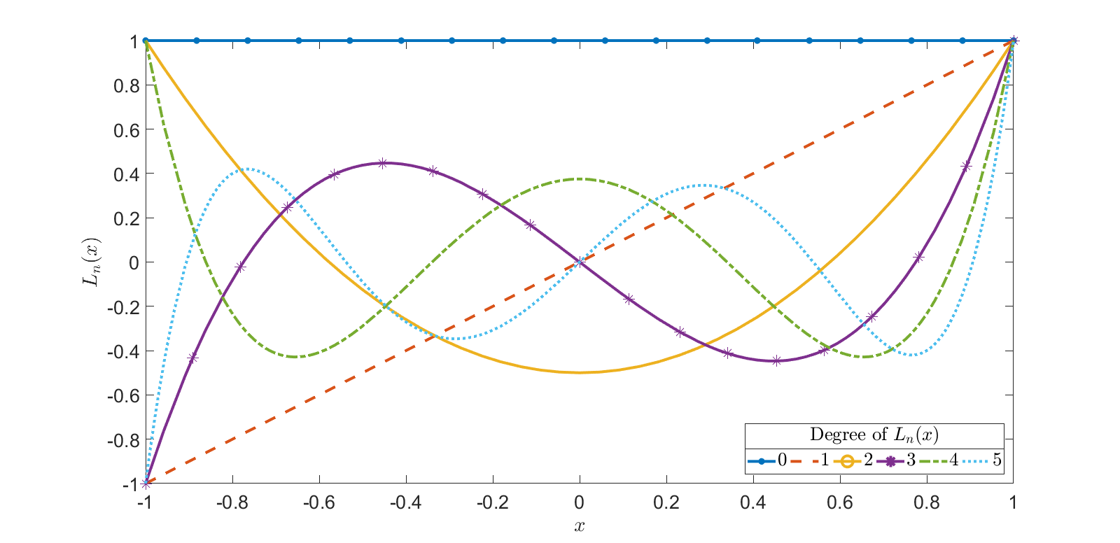
Figure 4.4: Legendre’s polynomials up to degree $5$.

In figure 4.4 we can see the first $6$ Legendre’s polynomials. The norm of Legendre’s polynomials is given by:

$$\|L_{n}(x)\|^{2}=\frac{2}{2n+1},$$ (4.44)

and an explicit formula for the derivative is

$$\frac{\mathrm{d}}{\mathrm{d}x}L_{n+1}(x)=(2n+1)L_{n}(x)+(2(n-2)+1)L_{n-2}(x)+(2(n-4)+1)L_{n-4}(x)+\dots$$ (4.45)

The proofs of these facts need more results from differential equations that would get us far from our purpose. We refer the interested reader to [66] and [106].

Returning to the original discussion, the new definition of the matrix in equation (4.28) is

$$\mathcal{M}_{i,j}=\left\langle L_{i},L_{j}\right\rangle_{I}.$$ (4.46)

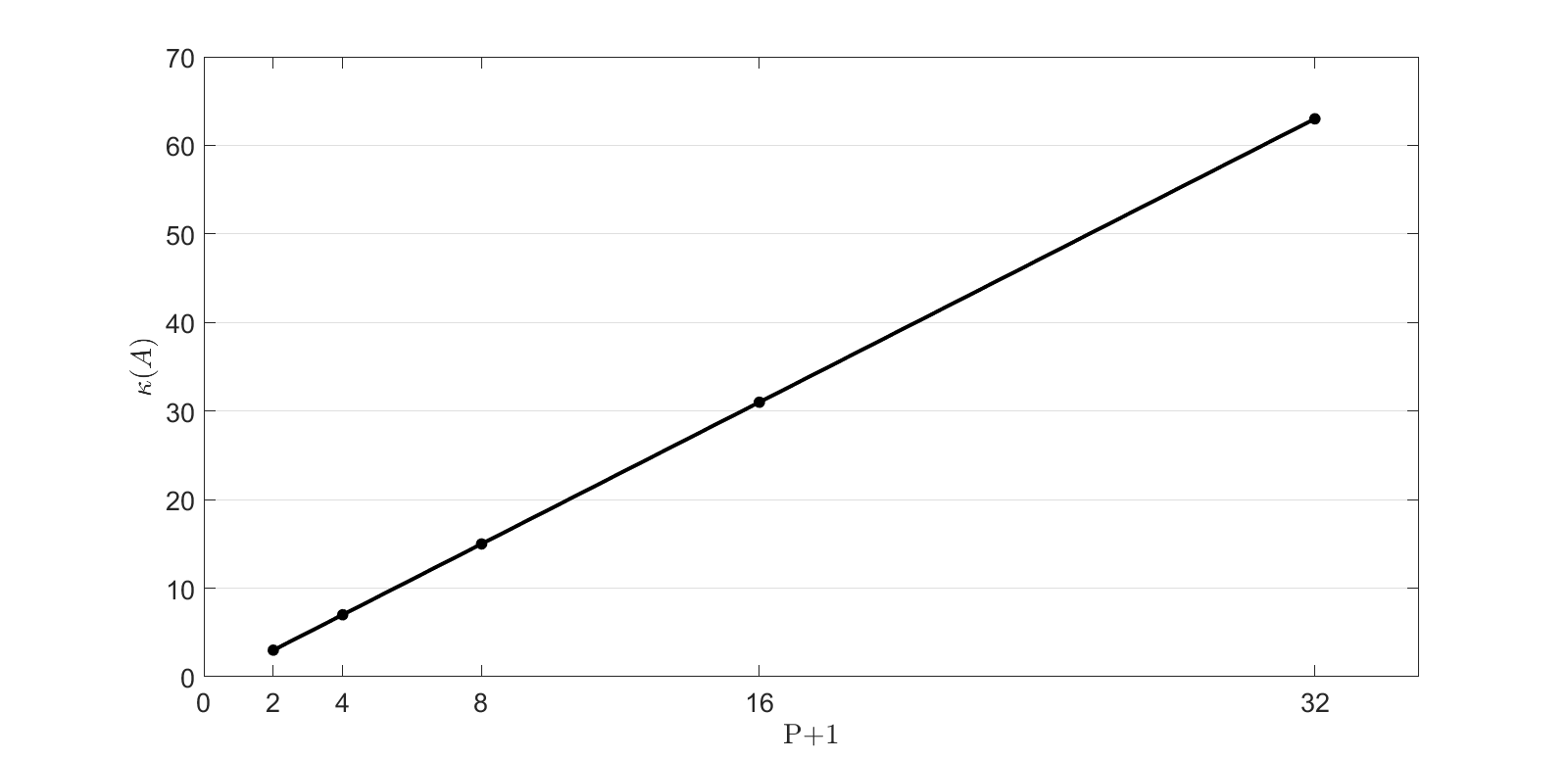
Figure 4.5: Condition number (in norm $1$) of the matrix $\mathcal{M}$. As we can see, it grows linearly.

In this case, as we would expect, the condition in norm $1$ of $\mathcal{M}$ is much smaller now, as we can appreciate in figure 4.5. We observe now a linear behaviour with respect to the matrix size, in opposition with the exponential when the canonical basis was used (figure 4.3). With this, we have solved what to do with the first term of equation (4.19). In the next subsection we will be dealing with the second term, the evaluation of the functions in the boundary of elements.

4.2.2 Numerical flux

We recall that the second term of equation (4.19) had the form

$$\left[\textbf{F}(\textbf{U})\cdot\boldsymbol{\psi}\right]_{x_{e}^{l}}^{x_{e}^{u}}.$$ (4.47)

Now we know that the test function will be a Legendre’s polynomial so, after resizing to local coordinates, in the boundary (that now will be either $-1$ or $1$) will have the values

$$L_{p}(\xi(x_{e}^{l}))=L_{p}(-1)=(-1)^{p},\qquad L_{p}(\xi(x_{e}^{u}))=L_{p}(1)=1.$$ (4.48)

The problem comes with $\textbf{F}(\textbf{U})$. This term is evaluated at the boundary of elements and hence, it carries the information between elements. But these values at the extremes of the elements may be not well defined, since although the solution is continuous at each element, it may not be continuous in $\mathcal{F}_{h}^{W}$. So, we have the problem (actually is a Riemann problem) of obtaining the value of the physical flux F at one point for which has two different values

$$\textbf{F}(\textbf{U}_{h}(x_{e}^{u},t))\neq\textbf{F}(\textbf{U}_{h}(x_{e+1}^{l},t)).$$ (4.49)

For convenience in the notation we will denote by

$$\textbf{U}_{L}=\textbf{U}_{h}(x_{e}^{u},t),\qquad\textbf{U}_{R}=\textbf{U}_{h}(x_{e+1}^{l},t)$$ (4.50)

the left and right solution at one interelement point, where $x_{e}\in\mathcal{F}_{h}^{W}$.

The way to solve this is approximating it with the aid of the so-called numerical flux $\textbf{H}(\textbf{U}_{L},\textbf{U}_{R})\colon\mathbb{R}^{2}\times\mathbb{R}^{2}\to\mathbb{R}^{2}$:

$$\textbf{F}(\textbf{U}_{h}(x_{e}^{u},t))\approx\textbf{H}(\textbf{U}_{L},\textbf{U}_{R})$$ (4.51)

In words, what we are doing is approximating a not well-defined function in the problematic point by a proper function that depends on the “left” and “right” values of the solution. Some desirable properties of the numerical flux are the following:

1. Continuity: $\textbf{H}(\ell,r)$ is Lipschitz-continuous with respect to $\ell,r$, i.e. there exists a constant $L_{H}>0$ such that

   $$\|\textbf{H}(\ell,r)-\textbf{H}(\ell^{*},r^{*})\|\leq L_{H}(\|\ell-\ell^{*}\|+\|r-r^{*}\|),$$ (4.52)

   where $\ell,r,\ell^{*},r^{*}\in\mathbb{R}^{2}$, for some norm $\|\cdot\|$.

2. Consistency: it works properly if we have usual continuity:

   $$\textbf{H}(c,c)=\textbf{F}(c)$$ (4.53)

   for $c\in\mathbb{R}^{2}$.

3. Conservativity: in higher dimensions, this condition means some kind of mass conservation. In one dimension it reduces to commutativity of the arguments:

   $$\textbf{H}(\ell,r)=\textbf{H}(r,\ell).$$ (4.54)

Apart from the aforementioned properties, there is no scientific agreement of which particular numerical flux to choose. In the next part we present some reasonable options.

Some choices of the numerical flux

One of the most intuitive options is the central numerical flux given by

$$\textbf{H}(\textbf{U}_{L},\textbf{U}_{R})=\frac{\textbf{F}(\textbf{U}_{L})+\textbf{F}(\textbf{U}_{R})}{2},$$ (4.55)

that is, an arithmetic mean of the left and right physical fluxes. But this numerical flux is unconditionaly unstable and, therefor, worthless for practical purposes (see [37]). In the most of applications, in which Navier-Stokes is included, it is suitable to use upwinding numerical fluxes. The concept of upwinding is based on the idea that the information on properties of a quantity is propagated in the flow direction. There is an abundance of schemes for this upwinding term — Vijagasundaram scheme, Steger-Warming scheme, VanLeer scheme or Osher-Solomon scheme are some examples that can be found in [37]. Further Riemann solvers can be found also in [118, 38, 46, 65, 125]. We have chosen and implemented two upwinding schemes mainly due to their simplicity and physical meaning. In the rest of the section we will give more details about these two schemes.

• The first one is a slight modification of the central numerical flux given in equation (4.55).

  $$\textbf{H}(\textbf{U}_{L},\textbf{U}_{R})=\frac{1}{2}\left[\textbf{F}(\textbf{U}_{L})+\textbf{F}(\textbf{U}_{R})-a(\textbf{U}_{R}-\textbf{U}_{L})\right],$$ (4.56)

  where $a$ is the local propagation speed and the direction is reflected in the difference $(\textbf{U}_{R}-\textbf{U}_{L})$ (since the wave propagates from left to right). The main idea is to use a centred flux to which just enough dissipation is added to ensure stability in all cases. In the scalar case the needed viscosity is given by the largest local wave speed (see [112]). With more components, there might be a superposition of the waves, each one with its corresponding eigenvalue. So taking the viscosity coefficient in the flux as the maximum over all eigenvalues should work. With this we have that

  $$a=\max_{\textbf{U}\in[\textbf{U}_{L},\textbf{U}_{R}]}\left|\lambda\left(\frac{\partial\textbf{F}(\textbf{U})}{\partial\textbf{U}}\right)\right|,$$ (4.57)

  that is, the maximum modulus of the eigenvalues of the jacobian matrix $\textbf{F}^{\prime}(\textbf{U})$.

  We will refer to the above flux as the Nessyahu and Tadmor (NT) central scheme [83]. It is most frequently called Lax-Friedrichs flux (although it is worth mentioning that such flux expression does not appear in Lax [72] but rather on Rusanov [102]).

• The second numeric flux is based on using the information provided by the method of characteristics. Since the characteristics are Riemann invariants, the solution should remain constant along these curves. We recall that the characteristics had the form

  $$W_{1,2}=u\pm 4\sqrt{\frac{\beta}{2\rho}}A^{1/4}$$ (4.58)

  and therefor

  $$A=\left(\frac{W_{1}+W_{2}}{4}\right)^{4}\left(\frac{\rho}{2\beta}\right)^{2},$$ (4.59)

  $$u=\frac{W_{1}+W_{2}}{2}.$$ (4.60)

  Since $W_{1}$ is the forward characteristic, it will need to get the information from the left, so if we denote

  $$\textbf{U}_{L}=\begin{bmatrix}A_{L}\\ u_{L}\end{bmatrix},\qquad\textbf{U}_{R}=\begin{bmatrix}A_{R}\\ u_{R}\end{bmatrix}$$ (4.61)

  we have that the upwinding forward characteristic is

  $$W_{1}^{\text{u}}=u_{L}+4\sqrt{\frac{\beta}{2\rho}}A_{L}^{1/4}.$$ (4.62)

  Analogously we have

  $$W_{2}^{\text{u}}=u_{R}-4\sqrt{\frac{\beta}{2\rho}}A_{R}^{1/4}.$$ (4.63)

  From here we build the upwinding variables

  $$A^{\text{u}}=\left(\frac{W_{1}^{\text{u}}+W_{2}^{\text{u}}}{4}\right)^{4}\left(\frac{\rho}{2\beta}\right)^{2},$$ (4.64)

  $$u^{\text{u}}=\frac{W_{1}^{\text{u}}+W_{2}^{\text{u}}}{2}.$$ (4.65)

  So, the numerical flux will be the physical flux applied to the upwinding variables, i.e.

  $$\textbf{H}(\textbf{U}_{L},\textbf{U}_{R})=\textbf{F}\left(\begin{bmatrix}A^{\text{u}}\\ u^{\text{u}}\end{bmatrix}\right)=\begin{bmatrix}u^{\text{u}}A^{\text{u}}\\ \frac{(u^{\text{u}})^{2}}{2}+\frac{p}{\rho}\end{bmatrix}.$$ (4.66)

  We can find this characteristic flux in the paper of Sherwin et al. [104].

To the best of our knowledge there is no theoretical analysis of this last flux (notice that it is done specifically for this problem). Regarding the NT flux there is some work on the stability of the method. We refer the interested reader to the aforecited references.

In this subsection we have dealt with points $x_{e}\in\mathcal{F}_{h}^{W}$, but the treatment of the inlet and outlet points $x_{e}\in\mathcal{F}_{h}^{io}$ is the same one. The only difference in this case would be, as one could expect

$$\textbf{U}_{L}=\textbf{U}_{\text{inflow}}$$ (4.67)

for the first element and

$$\textbf{U}_{R}=\textbf{U}_{\text{outflow}}$$ (4.68)

for the last element. Since we are in the case of nonlinear hyperbolic systems, as we can read in [30], the theory for the boundary conditions is missing.

In this chapter we have achieved the semi-discrete scheme:

$$\begin{split}\overbrace{\frac{2}{2p+1}\frac{\partial\hat{\textbf{U}}_{p}(t)}{\partial t}}^{\textrm{Subsection }\ref{subsec:test}}=\frac{2}{x_{e}^{u}-x_{e}^{l}}\int_{I}\left[\textbf{F}(\textbf{U}(\xi,t))\cdot\overbrace{L_{p}^{\prime}(\xi)}^{\textrm{Equation }\eqref{eq:derleg}}+\textbf{T}(\textbf{U}(\xi)L_{p}(\xi)\right]\mathrm{d}\xi\\ \underbrace{+(-1)^{p}\textbf{H}(\textbf{U}_{h}(x_{e}^{l},t),\textbf{U}_{h}(x_{e-1}^{u},t))-\textbf{H}(\textbf{U}_{h}(x_{e}^{u},t),\textbf{U}_{h}(x_{e+1}^{l},t))}_{\textrm{Subsection }\ref{subsec:flux}},\end{split}$$ (4.69)

for the Legendre degree $p=0,\dots,P$ and for every element $\Omega_{e}$, $e=1,\dots,N_{\textrm{el}}$. In order to obtain a discrete algorithm we need a quadrature rule for the integral and a scheme for evolve in time. In the next chapter, the chosen rules will be explained, along with some implementation details. Some numerical results are also presented in the following chapter.

Chapter 5 Implementation and results

In this chapter we fully discretise the semi-discrete method previously presented. In order to achieve this, we present the quadrature rules used for the spatial and temporal integration. In the second part of this chapter we present some results of applying this method. We have studied its stability, convergence and sensitivity to parameters carrying out a total of nearly $2000$ simulations.

5.1 Spatial integration

With all we have done in this section, we have a semi-discrete method given by equation (4.19). But for the implementation of the method, we need to evaluate the integrals

$$\left\langle\textbf{F}(\textbf{U}),\boldsymbol{\psi}_{x}\right\rangle_{\Omega_{e}} =\frac{2}{x_{e}^{u}-x_{e}^{l}}\left\langle\textbf{F}(\textbf{U}),\psi_{x}\right\rangle_{I}=\frac{2}{x_{e}^{u}-x_{e}^{l}}\int_{-1}^{1}\textbf{F}(\textbf{U}(\xi,t))\cdot L_{p}^{\prime}(\xi)\mathrm{d}\xi,$$ (5.1)

$$\left\langle\textbf{T}(\textbf{U}),\boldsymbol{\psi}\right\rangle_{\Omega_{e}} =\frac{2}{x_{e}^{u}-x_{e}^{l}}\int_{-1}^{1}\textbf{T}(\textbf{U}(\xi,t))\cdot L_{p}(\xi)\mathrm{d}\xi.$$ (5.2)

The quadrature rule chosen, following the steps of [104] has been the Legendre-Gauss-Lobatto (LGL) quadrature. First we need to define the Gaussian integration:

Definition 1 (Gaussian integration).

Let $x_{0},\dots,x_{N}$ be the roots of the $N+1$-th orthogonal polynomial $p_{N+1}$, and let $w_{0},\dots,w_{N}$ be the solution of the linear system

$$\sum_{j=0}^{N}(x_{j})^{k}w_{j}=\int_{-1}^{1}x^{k}w(x)\mathrm{d}x,\qquad 0\leq k\leq N,$$ (5.3)

where $w(x)\colon A\to\mathbb{R}^{+}$ is some weight function, where $A\subset[-1,1]$ is a discrete set. The positive numbers $w_{j}$ are called weights.

Then,

Proposition 7.

The following properties are satisfied:

1. $$\sum_{j=0}^{N}p(x_{j})w_{j}=\int_{-1}^{1}p(x)w(x)\mathrm{d}x$$ (5.4)

   for all $p\in\mathcal{P}_{2N+1}(I)$ where $I=[-1,1]$.

2. It is not possible to find $x_{j}$, $w_{j}$, $j=0,\dots,N$ such that (5.4) holds for all polynomials $p\in\mathcal{P}_{2N+2}(I)$.

The proofs can be found in [26]. This version of Gauss integration is quite well known. However, the roots, which correspond to the collocation points, are all in the open interval $]-1,1[$. The requirement of imposing boundary conditions at one or both end points creates the need for the generalised Gauss integration formulas which include these points. This lead us to the Gauss-Lobatto integration:

Definition 2 (Gauss-Lobatto integration).

Let $-1=x_{0},x_{1},\dots,x_{n}=1$ be $N+1$ roots of the polynomial

$$q(x)=p_{N+1}(x)+ap_{N}(x)+bp_{N-1}(x),$$ (5.5)

where $a$ and $b$ are chosen so that $q(-1)=q(1)=0$. Let $w_{0},\dots,w_{N}$ be the solution of the linear system

$$\sum_{j=0}^{N}(x_{j})^{k}w_{j}=\int_{-1}^{1}x^{k}w(x)\mathrm{d}x\qquad 0\leq k\leq N.$$ (5.6)

Then

$$\sum_{j=0}^{N}p(x_{j})w_{j}=\int_{-1}^{1}p(x)w(x)\mathrm{d}x,$$ (5.7)

for all $p\in\mathcal{P}_{2N-1}(I)$.

In the special case of Jacobi weight, i.e. $w(x)=(1-x)^{\alpha}(1+x)^{\beta}$ with $\alpha,\beta\in[-1/2,1/2]$ there is an alternative characterisation of the Gauss-Lobatto points, namely they are the points $-1$, $+1$ and the roots of the polynomial

$$q(x)=p^{\prime}_{N}(x).$$ (5.8)

For the proofs of the aforementioned results see [17]. With this, if we choose $p_{N}=L_{N}$ the $n$-th Legendre we obtain the Legendre-Gauss-Lobato quadrature. Since explicit formulas for the quadrature nodes are not known to the best of our knowledge, such points have to be computed numerically as zeroes of appropriate polynomials. The quadrature weights can be expressed in closed form in term of the nodes, as indicated in the following formulas (see, e.g., Davis and Rabinowitz [26]):

$$x_{0}=-1,x_{N}=1,\{x_{j}\}_{j=1}^{N-1}\text{ zeroes of }L_{N}^{\prime};$$ (5.9)

$$w_{j}=\frac{2}{N(N+1)}\frac{1}{[L_{N}(x_{j})]^{2}}\qquad j=0,\dots,N.$$ (5.10)

Some points and weights are presented in table 5.1.

Number of nodes	Nodes	Weights
$1$	$0$	$2$
$2$	$\pm\sqrt{\frac{1}{3}}\approx\pm 0.58$	$1$
$3$	$0$	$\frac{8}{9}\approx 0.89$
	$\pm\sqrt{\frac{3}{5}}\approx\pm 0.77$	$\frac{5}{9}\approx 0.56$
$4$	$\pm\sqrt{\frac{3}{7}-\frac{2}{7}\sqrt{65}}\approx\pm 0.34$	$\frac{18+\sqrt{30}}{36}\approx 0.65$
	$\pm\sqrt{\frac{3}{7}+\frac{2}{7}\sqrt{65}}\approx\pm 0.86$	$\frac{18-\sqrt{30}}{36}\approx 0.35$
$5$	$0$	$\frac{128}{225}\approx 0.57$
	$\pm\frac{1}{3}\sqrt{5-2\sqrt{\frac{10}{7}}}\approx\pm 0.54$	$\frac{322+13\sqrt{70}}{900}\approx 0.48$
	$\pm\frac{1}{3}\sqrt{5+2\sqrt{\frac{10}{7}}}\approx\pm 0.90$	$\frac{322+13\sqrt{70}}{900}\approx 0.24$

Table 5.1: Points and weights for the Legendre-Gauss-Lobatto quadrature in $[-1,1]$.

With this, we have the final discrete algorithm

$$\begin{split}\overbrace{\frac{2}{2p+1}\frac{\partial\hat{\textbf{U}}_{p}(t)}{\partial t}}^{\textrm{Subsection }therefor{subsec:test}}=\overbrace{\frac{2}{x_{e}^{u}-x_{e}^{l}}\int_{I}\left[\textbf{F}(\textbf{U}(\xi,t))\cdot\underbrace{L_{p}^{\prime}(\xi)}_{\textrm{Equation }\eqref{eq:derleg}}+\textbf{T}(\textbf{U}(\xi)L_{p}(\xi)\right]\mathrm{d}\xi}^{\textrm{Subsection }\ref{subsec:int}}\\ \underbrace{+(-1)^{p}\textbf{H}(\textbf{U}_{h}(x_{e}^{l},t),\textbf{U}_{h}(x_{e-1}^{u},t))-\textbf{H}(\textbf{U}_{h}(x_{e}^{u},t),\textbf{U}_{h}(x_{e+1}^{l},t))}_{\textrm{Subsection }\ref{subsec:flux}},\end{split}$$ (5.11)

for the Legendre degree $p=0,\dots,P$ and for every element $\Omega_{e}$, $e=1,\dots,N_{\textrm{el}}$. We have not mentioned it, but regarding the initial condition we need to transform it to its degrees of freedom. Following the reasoning of the previous chapter, if $\textbf{U}_{0}(x)=\textbf{U}(x,0)$ we have

$$\frac{2}{2p+1}\left(\hat{\textbf{U}}_{0}\right)_{p}=\int_{I}\textbf{U}_{0}(\xi)L_{p}(\xi)\mathrm{d}\xi$$ (5.12)

for $p=0,\dots,P$. This result was also obtained by [117].

5.2 Temporal integration

We have obtained an algorithm for getting the derivatives of the degrees of freedom. Hence, we need a scheme to evolve in the temporal dimension. We will only recover the physical solution when the simulation is done (in order to plot the solution) using equation (4.23). In most of the applications a Runge-Kutta of order $2$ or $3$ is enough, but following [103] we have chosen the Adams-Bashforth scheme. These methods were designed by Adams to solve a differential equation modelling capillary action due to Bashforth in [11]. The main reasons of this election are, on one hand, the implementation-friendly expression; and on the other hand, the fact that the Adams-Bashforth method with $s$ steps has order $s$. This will allow us to rise the order if it is desired.

This scheme is encompassed in the so-called linear multistep methods. Conceptually, multistep methods attempt to gain efficiency by keeping and using the information from previous steps rather than discarding it (as Euler explicit, for example). Moreover, in the case of linear multistep methods, a linear combination of the previous points and derivative values is used. Using our notation, denoting the iteration by superscripts, a linear multistep method has the form

$$\hat{\textbf{U}}^{n+s}+a_{s-1}\cdot\hat{\textbf{U}}^{n+s-1}+a_{s-2}\cdot\hat{\textbf{U}}^{n+s-2}+\dots+a_{0}\cdot\hat{\textbf{U}}^{n}$$ (5.13)

$$=\Delta t\cdot\left(b_{s}\cdot\hat{\textbf{U}}_{t}^{n+s}+b_{s-1}\cdot\hat{\textbf{U}}_{t}^{n+s-1}+\dots+b_{0}\cdot\hat{\textbf{U}}_{t}^{n}\right)$$ (5.14)

where the coefficients $\{a_{i}\}_{i=0}^{s-1}$ and $\{b_{i}\}_{i=0}^{s}$ determine the method, $\hat{\textbf{U}}^{0}=\hat{\textbf{U}}_{0}$ and $\Delta t$ is the time step. In the case of the Adams-Bashforth methods, they are explicit methods and hence $a_{s-1}=-1$ and $a_{s-2}=\dots=a_{0}=0$. Regarding the other coefficients, the main idea is to interpolate the derivatives using the Lagrange formula for polynomial interpolation. This yields the expression for the coefficients

$$b_{s-j-1}=\frac{(-1)^{j}}{j!(s-j-1)!}\int_{0}^{1}\prod^{s-1}_{\begin{subarray}{c}i=0\\ i\neq j\end{subarray}}(u+i)\mathrm{d}u,$$ (5.15)

for $j=0,\dots,s-1$. It can be shown that with this construction the $s$-step Adams-Bashforth method has order $s$ (see [58]).

In the following sections some numerical results have been performed using this discrete method presented along this chapter and the previous one. All the simulations have been done in Matlab R2017a.

5.3 Test case

As a test case we have replicated one of the numerical experiments done by [104]. We consider a normalised vessel of unit area, $A_{0}=1$ and normalise the mean velocity so that it has a unit value too ($u_{0}=1$). Physiologically we expect the wave speed to be an order of magnitude higher than the mean velocity and so we prescribe a mean wave speed of $c_{0}=\sqrt{\beta/(2\rho)}A_{0}^{1/4}=10$. This can be achieved by selecting $\beta=100$ and $\rho=0.5$. As inflow velocity we use an analytic function simulating the heart beat of the form

$$u_{\textrm{inflow}}(t)=1-0.4\sin(wt)-0.4\sin(2wt)-0.2\cos(2wt)$$ (5.16)

where $w=2\pi/T$ and $T$ is the time period (see figure 5.1).

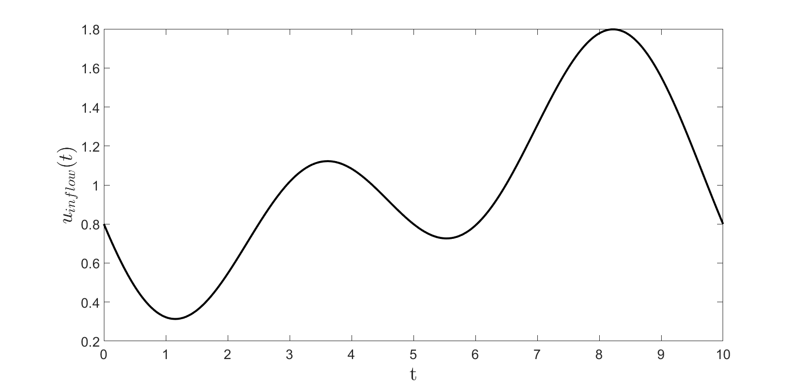
Figure 5.1: Inflow velocity in the same units as the initial velocity.

Making the assumption that the spatial wavelength $\lambda$ is approximately $100$ times larger than the vessel diameter, we choose a time span of $10$ since for the linear case $\lambda\approx 100$.

Since we are considering a problem with a wavelength of $\lambda=100$, in order to observe the wave as a function of the artery centreline we will consider a computational interval $[-100,100]$. The domain is subdivided into $N_{\textrm{el}}=10$ elements of equal length and a polynomial order of $P=7$ is applied within each element. We impose the boundary conditions of

$$u_{l}(-100,t) =u_{\textrm{inflow}}(t), u_{r}(100,t) =1,$$ (5.17)

$$A_{l}(-100,t) =1, A_{r}(100,t) =1.$$ (5.18)

A second-order time stepping scheme was applied with a time step of $\Delta t=5\cdot 10^{-3}$.

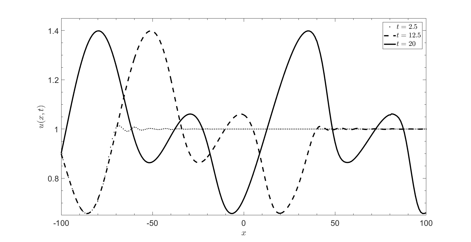
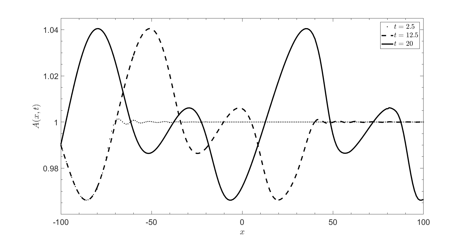
Figure 5.2: Advection of travelling waves at times $t=2.5$, $t=12.5$, $t=20$.

In figure 5.2 we can see how, indeed, we obtain the same results and a travelling wave appears.

Both in these simulations and henceforth, the numerical flux used was the characteristic flux presented in 4.2.2. The plots have been repeated for the NT flux and no significant differences have been observed.

5.4 Convergence and stability

Regarding the stability and convergence of the method, there is not so much in the literature. We can find some partial results about stability (specially for nodal DG) in [64, 95, 48]. In these papers some CFL conditions are given, but for specific problems. Hence, in general, their conclusions can not be extrapolated. In order to obtain a rough idea of the stability of this method for our problem, we have performed some simulations.

$N_{\textrm{el}}$	$1,\dots,8$	$\beta$	$2.2\cdot 10^{4}$
$P$	$0,\dots,9$	$BPM$	$80$
$\Delta t$	$10^{-4}:5\cdot 10^{-4}:10^{-2}$	Final time	$5$ seconds

Table 5.2: Parameters’ values for the stability experiment.

In table 5.2 we can see the parameters used for the simulation. For the time step we have used Matlab notation (ini:step:end). Following the measures used in subsection 3.2.1 and appendix A we have estimated $A_{0}=A_{\text{outflow}}=A_{\text{inflow}}=4\cdot 10^{-2}$ and $u_{0}=u_{\text{outflow}}=1$. The other parameters have the same values as in the previous simulations. Therefor, the conclusions obtained are based on $1600$ simulations. What we have observed is that, in every case, no matter the polynomial degree, number of elements (and hence space grid refinement), or time step the solution obtained is completely stable, i.e., we have not observed neither oscillations nor divergence. Hence we cannot state any kind of CFL condition relating $\Delta t$ with $N_{\textrm{el}}$. We remark that these are great results, since from a clinical point of view (due to the reasonable choice of the parameters) the method is stable.

With the convergence of the method we have a similar situation. Some works have been made in this line, see [69, 60], but for specific (and scalar) equations. Nevertheless, it is well known that FEMs are chosen for their accuracy (see [78]), and this feature is inherited by DG-FEM. Moreover, in our case we have an additional problem: the boundary conditions. For reproducibility we have considered the same inlet data as [104], a periodic function where we can control the beats per minute. But, because of the form how it is constructed, it is not immediate its manipulation. Due to this, we can not compare it with real data to measure the real error.

What we can do is to measure how discontinuous is the discontinuous Galerkin method. For fixed parameters (the same ones as in the previous simulations, unless otherwise indicated) we have refined the mesh, i.e., we have augmented the number of elements $N_{\textrm{el}}$ from two to eight. As a measure of discontinuity we have considered the norm infinity of the differences between the left and right values of blood flow velocity at each element boundary. We have considered a $5$ seconds simulation, measuring approximately at first, at the middle and at the end of the simulation. Since depending on the time step, each simulation has a variable number of iterations we have specified this value in the variable It.

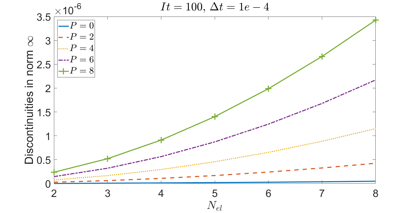
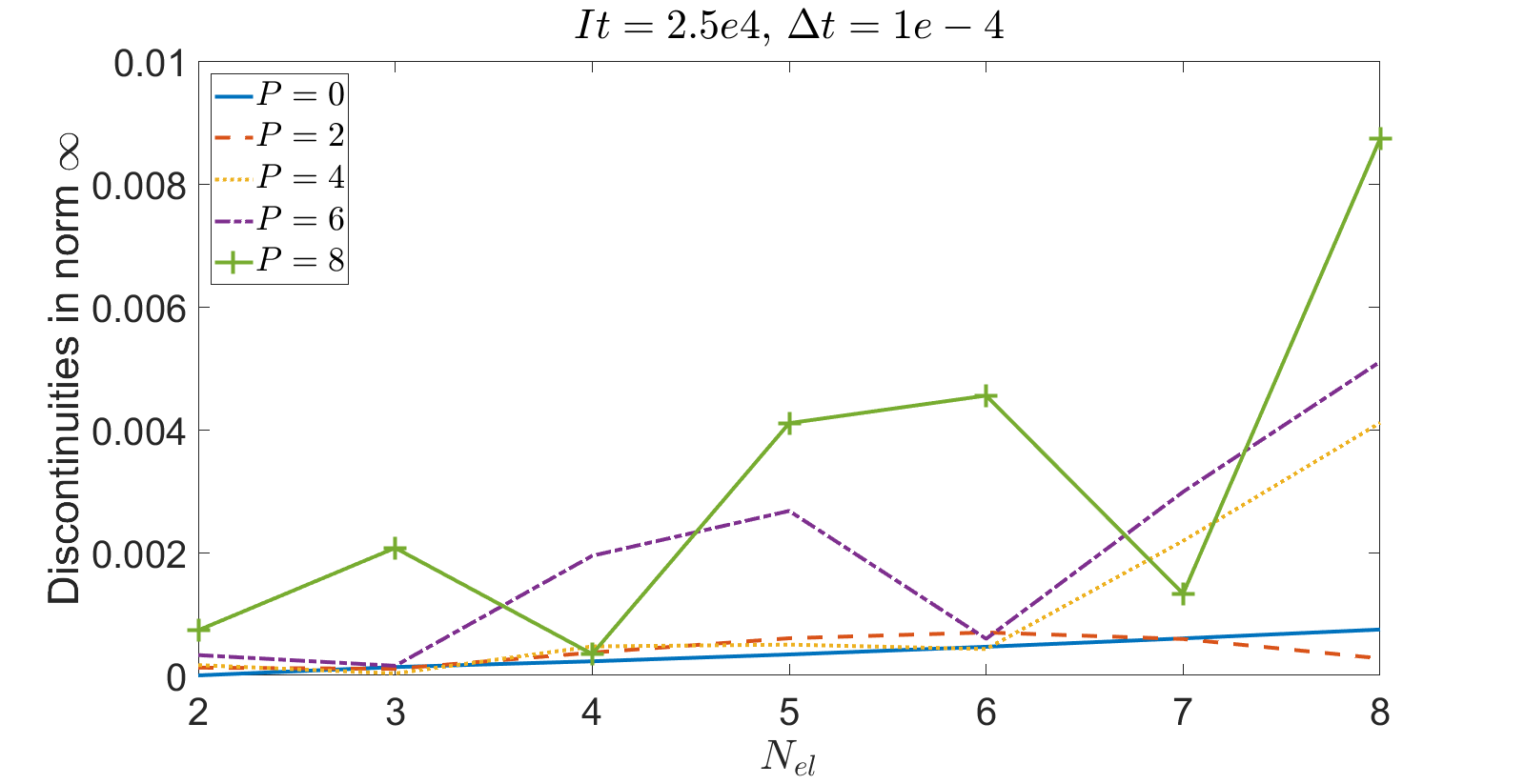
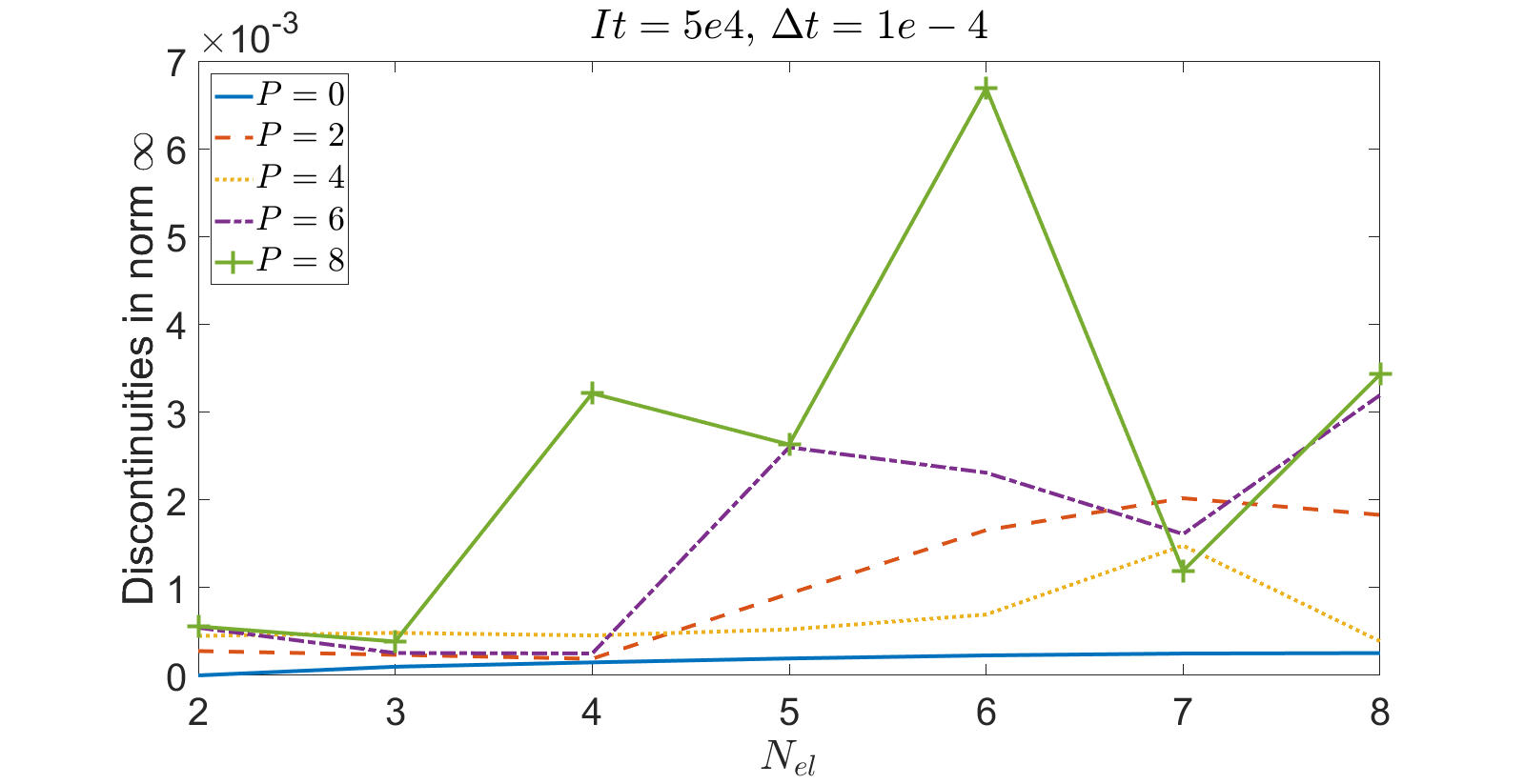
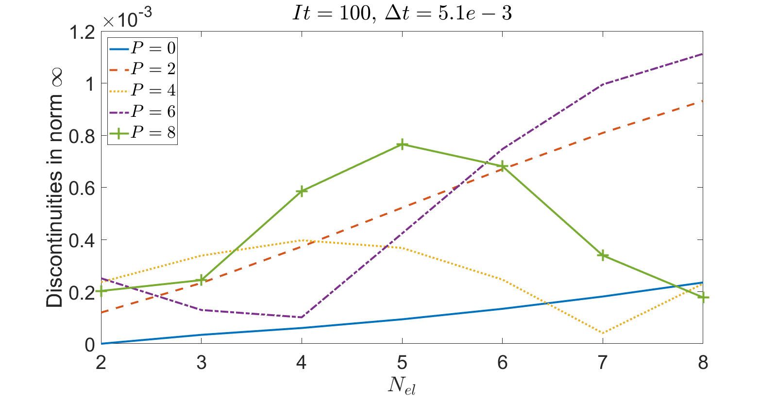
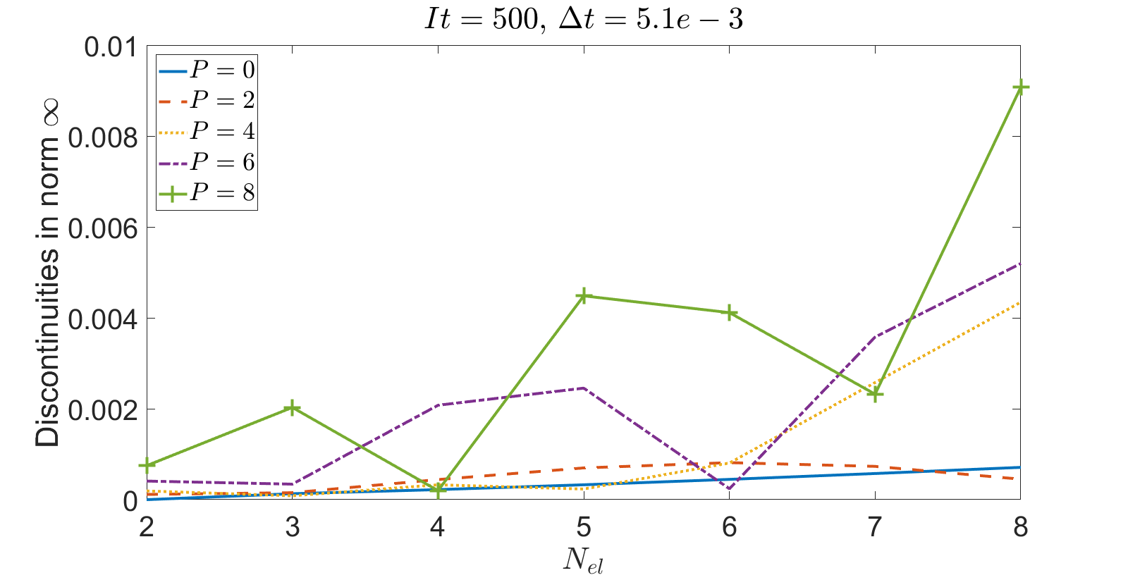
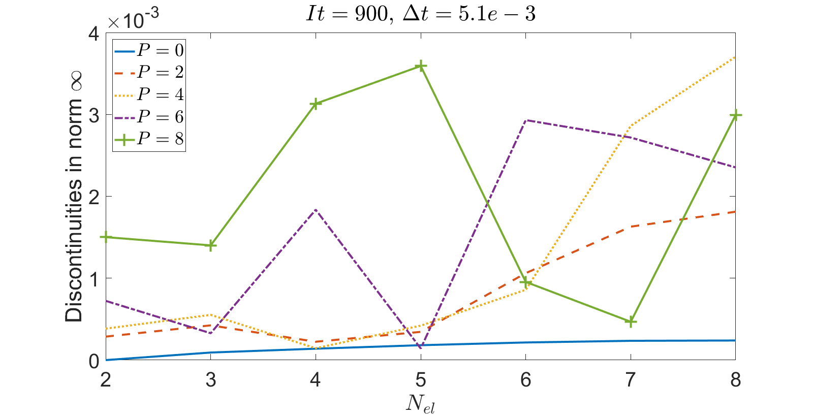
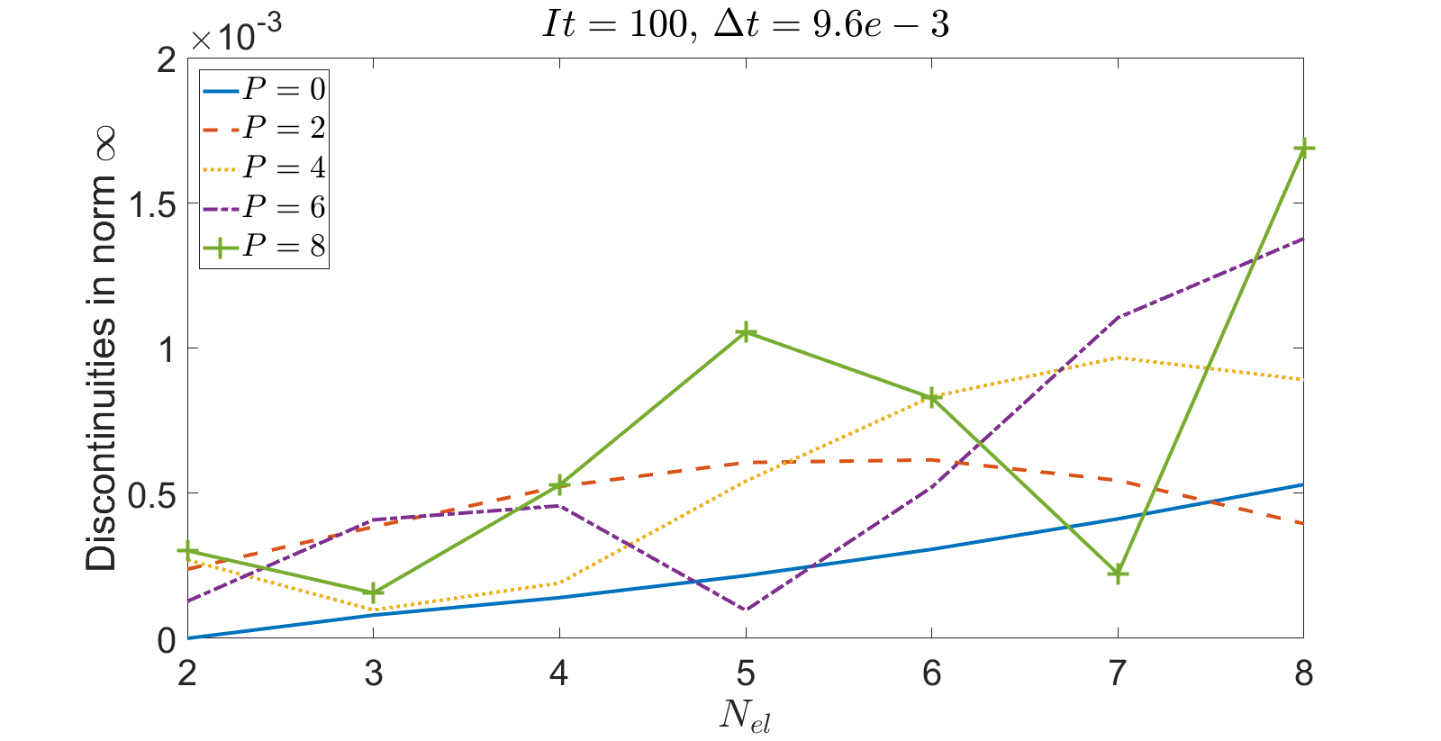
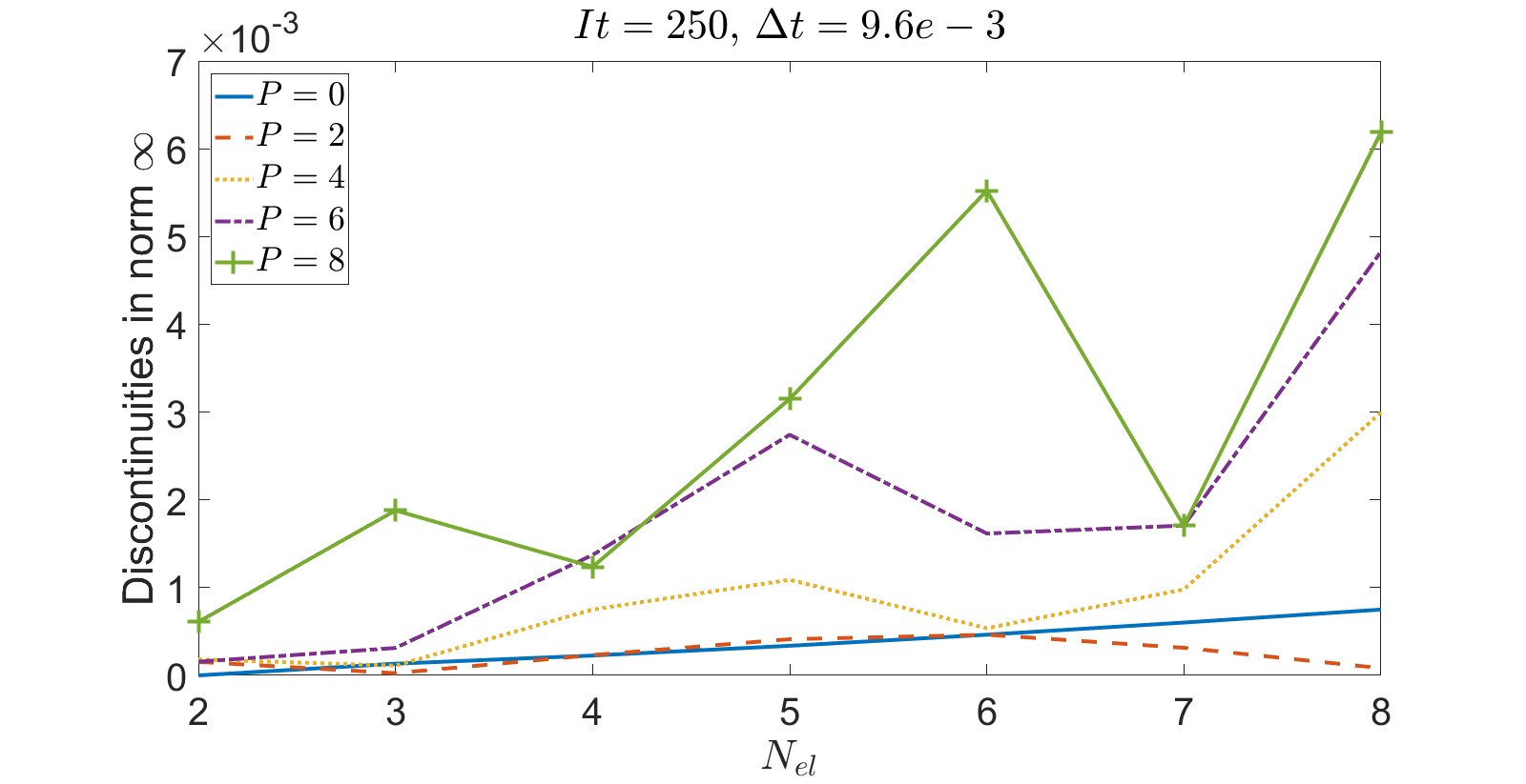
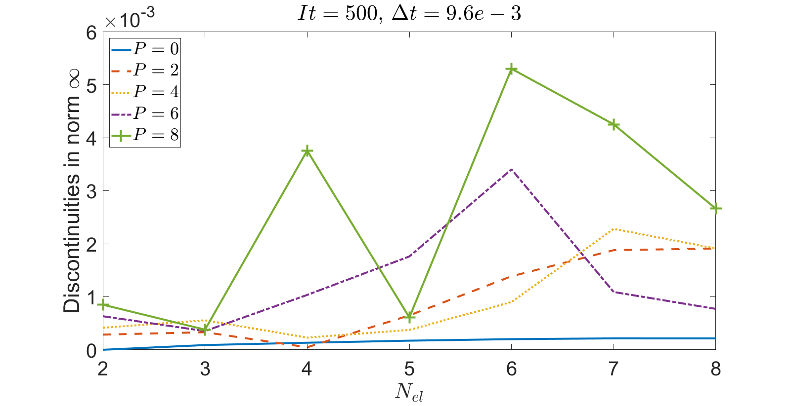
Figure 5.3: Discontinuity measure varying $N_{\textrm{el}}$, $\Delta t$, $P$ and the time when it is measured.

We present the results in figure 5.3. As it can be seen, there is not a clear pattern from which some assertion can be done. It seems that the higher is the number of elements, the higher are the discontinuities. This may be caused due to the freedom of the polynomial to oscillate when it has a higher degree. Nevertheless, we notice that the magnitudes are insignificant. We recall that the rest blood velocity was $1$ m/s.

5.5 Biomedical simulations dependent on the parameters

The next result we show is how the variables change depending on the physical parameters. As independent variables we have chosen two parameters of our model. The first parameter is $\beta$, which embraces the physical properties of the vessel’s wall. Following the measures used in subsection 3.2.1 and appendix A we have estimated a reasonable range of $\beta\in[15\cdot 10^{3},30\cdot 10^{3}]$. The second variable we have controlled is the inflow data. We have used the aforementioned inflow function for velocity but now controlling the period $T$. Since it is the periodicity of the wave, biologically it means the heart beats per second. We have done simulations for $T\in[0.8,2]$ which correspond to values of beats per minute (in what follows, BPM) between $48$ and $120$.

As dependent variables we have considered the maximum value of the flow velocity and vessel amplitude. These simulations are done in a time span of $5$ seconds with a time step of $0.005$. The spatial discretisation has been of $10$ elements with polynomials of degree $5$.

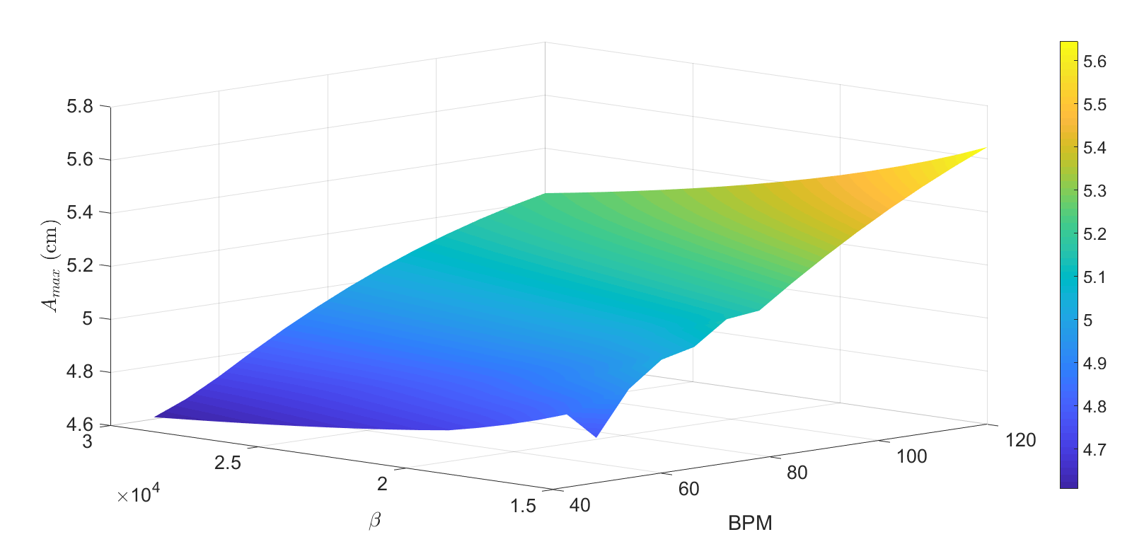
Figure 5.4: Maximum arterial amplitude (in centimetres) as a function of the BPM and $\beta$.

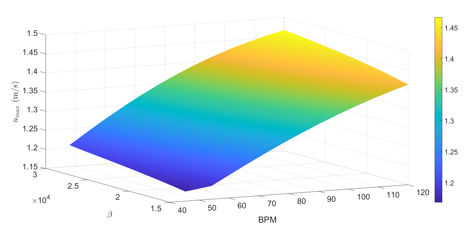
Figure 5.5: Maximum blood flow velocity (in m/s) as a function of the BPM and $\beta$.

Several conclusions are obtained from these plots. The most notorious is maybe the clear growth of both quantities as the heart rate rises. This is what we could expect since the greater is the heart rate, the faster is the blood velocity. Also, if we augment the BPM, the inflow blood acceleration $u_{\textrm{inflow}}^{\prime}$ also rises. This is the reason why the walls need to expand.

Regarding the dependence on $\beta$, the inverse behaviour is observed between the two quantities. Nevertheless, this also makes sense because the greater is $\beta$, the more rigid is the wall. This can be achieved by rising Young’s modulus or making more compressible the material, shrinking Poisson’s ratio. In both cases, more effort will have to be done to displace the wall, as we observe in figure 5.4. In order to conserve the flux, if the amplitude gets smaller, the blood velocity must be greater. Indeed, this is what can be observed in figure 5.5.

The magnitudes are also coherent with the physical meaning. In the case of the amplitude we see how the greatest difference is about one centimetre (we recall that the rest amplitude was of $4$ cm). With the velocity, the difference is similar, since the initial velocity was of $1$ m/s and the values are between $1.15$ and $1.45$ m/s.

Chapter 6 Conclusions and future work

In this work we have carried out an analysis of a blood flow model in elastic arteries, based on the Navier-Stokes equations. Starting from a short historical survey, we have stated the equations for our model. We have treated them from a more abstract mathematical point of view to extract some results about the arterial behaviour. In the second part of this work we have focused on the numerical method for the simulations, and its deduction. We have ended with a short analysis of this method and with some numerical tests. Next we review the main aspects that have been treated during the text.

As the reader has been able to see, four paradigms have merge along the whole document:

• A small survey point of view. Chapter 1 has been presented as a historical background on arterial mechanics, up to $20$^th century. In subsection 2.1.3 the main models for one dimensional artery simulation have been enumerated, situating them chronologically. At the rest of the document, a distinguished amount of references has been cited in order to either justify assumptions or avoid digressions.

• Common reasonings in physics. Starting from physical principles such as Newton’s second law, we have derived more complex mathematical relations in terms of partial derivative equations, as have been done in chapter 2. Once the equations have been established, conclusions have been extracted directly from these equations, such us the conservation of physical quantities.

• Mathematical, academic analysis. In chapter 3 we have presented more abstract results, suitable in calculus areas. Although, as we specified in the introduction, the objective of the work is the blood simulation, we have considered necessary this part. This analysis has made possible to ensure some necessary conditions for the feasibility of the model, such as the non-collapse of the artery. We recall that in subsection 3.2.1 a explicit time and place for the appearance of a shock wave has been obtained. This theorem is an original result of this work based on a slightly different model presented by [15]. This result has been published in $2017$ in the 4º Congreso de jóvenes investigadores (IV Conference for young researchers) (see [101])

• Biomedical based numerical performance. Using the data presented in appendix A and the numerical scheme of Discontinuous Galerkin (chapter 4) some simulations have been performed. Although some wave simulations had been done in [104] among others, this kind of simulations have not been performed, to the best of our knowledge.

Nevertheless, some lines of future work have been opened and this field of knowledge continues proliferating. The step to three dimensional models has already been made, as in [39]. Even though we have not explain it for avoiding complexity, bifurcations are also possible as is explained in [104]. Maybe one of the most promising branches is coupling the arterial simulation with fractional calculus, as was illustrated in subsection 2.1.3. This is useful where more viscoelastic behaviours appear, such as in capillaries, aneurysms or simulation of arterial valves. See for example [29, 25, 132, 89]. More recent are the works of Perdikaris et al. simulating large arterial network using blood flow models together with fractal-tree closures [88].

Some possible lines of future work are the following:

1. Using realistic inflow data. We have used analytic, explicit functions for the inflow data, but maybe real measures are more appropriate for validating the model. Moreover, instead of using averaged data, personalised measures would be interesting for the usefulness of the model. Thus we could predict some diseases or check the consequences of some medical procedures.

2. Stochastic analysis. In this work we have performed some basic sensitivity analysis of the main parameters of the model. But, as a quick observation in the literature offers, there is a great variability in the values of biophysical parameters. Because of this uncertainty, some stochastic analysis would be interesting, either with the point of view of statistics, or from the random differential equations’ point of view.

3. Characterisation of different diseases. From aneurysm to blood thickening or aorta insufficiency, there are some conditions that could be modelled with blood flow simulations. This could provide some characterisation of such diseases and improving their understanding.

4. In a more mathematical field, necessary and sufficient conditions for smooth flow. Moreover, if these conditions had biophysical meaning, they would be of a great usefulness.

Appendix A Biological parameters

In this appendix, following the suggestions of [110] we enumerate some biologically-realistic values for the 1D flow model parameters in the context of simulationg blood flow in large vessels.

1. Blood mass density ($\rho$): $1050\text{kg}\cdot\text{m}^{-3}$. [39, 108, 73, 9, 8, 15, 109, 63, 7].

2. Blood dynamic viscosity ($\mu$): $0.0035\text{N}/(\text{s}\cdot\text{m}^{2})$.[39, 108, 73, 9, 8, 63, 59, 2, 40, 4, 127, 27]

3. Young’s elastic modulus ($E$): $10^{5}\text{N}/\text{m}^{2}$. [39, 73, 9, 8, 59, 2, 40, 27, 41, 133, 134, 75, 14, 56, 28].

4. Vessel wall thickness ($h_{0}$): this, preferably, is vessel dependent, i.e. a fraction of the vessel radius according to some experimentally-established mathematical relation. For arteries, the typical ratio of wall thickness to inner radius is about $0.1-0.15$, and this ratio seems to go down in the capillaries and arterioles. Therefor a typical value of $0.1$ seems reasonable.[39, 73, 40, 133, 90, 13, 122, 9, 121].

5. Momentum correction factor ($\alpha$): assuming Newtonian flow, about $4/3$ would give a parabolic profile, while with $1$ we would get a flat profile. An intermediate value, e.g. $1.2$, may be used to account for non-Newtonian shear-thinning effects [108, 73, 15, 40, 103, 41, 86, 42].

6. Poisson’s ratio ($\nu$): $0.45$ [39, 9, 8, 59, 27, 41, 133, 14, 28, 103, 94].

References

- [1] M. B. Abbott. An Introduction to the Method of Characteristics. Thames and Hudson, 1966.
- [2] J. Alastruey, K. H. Parker, J. Peiro, and S. Sherwin. Lumped parameter outflow models for 1-d blood flow simulations: Effect on pulse waves and parameter estimation. Communications in Computational Physics, 4:317–336, 08 2008.
- [3] M. Anliker, R. L. Rockwell, and E. Ogden. Nonlinear analysis of flow pulses and shock waves in arteries. Zeitschrift für angewandte Mathematik und Physik ZAMP, 22(3):563–581, 1971.
- [4] L. Antiga. Patient-Specific Modeling of Geometry and Blood Flow in Large Arteries. PhD thesis, Milan Polytechnic, 2002.
- [5] F. Aràndiga and P. Mulet. Càlcul Numèric, volume 109. Servei de Publicacions de la Universitat de València, 2008.
- [6] F. Aràndiga, P. Mulet, and R. Donat. Mètodes Numèrics per a l’àlgebra lineal, volume 39. Servei de Publicacions de la Universitat de València, 2000.
- [7] H. Ashikaga, B. Coppola, K. Yamazaki, F. Villarreal, J. Omens, and J. Covell. Changes in regional myocardial volume during the cardiac cycle: implications for transmural blood ow and cardiac structure. American Journal of Physiology - Heart and Circulatory Physiology, 295(2):H610–H618, 2008.
- [8] A. P. Avolio. Multi-branched model of the human arterial system. Medical and Biological Engineering and Computing, 18(6):709–718, Nov 1980.
- [9] S. Badia, A. Quaini, and A. Quarteroni. Coupling biot and navier-stokes problems for fluid-poroelastic structure interaction. Journal of Computational Physics, 228(21):7986–8014, 08 2009.
- [10] T. J. Barth and P. O. Frederickson. Higher order solution of the euler equations on unstructured grids using quadratic reconstruction. AIAA paper, 90:0013, 1990.
- [11] F. Bashforth and J. C. Adams. An attempt to test the theories of capillary action by comparing the theoretical and measured forms of drops of fluid. With an explanation of the method of integration employed in constucting the tables which give the theoretical forms of such drops. Cambridge University Press, 1883.
- [12] K.-J. Bathe. Finite element procedures. Klaus-Jurgen Bathe, 2006.
- [13] W. Blondel, B. Lehalle, M.-N. Lercher, D. Dumas, D. Bensoussan, and J.-F. Stoltz. Rheological properties of healthy and atherosclerotic human arteries. Biorheology, 40(1–3):369–376, 2003.
- [14] V. M. Calo, N. F. Brasher, Y. Bazilevs, and T. J. R. Hughes. Multiphysics model for blood flow and drug transport with application to patient-specific coronary artery flow. Computational Mechanics, 43(1):161–177, Dec 2008.
- [15] S. Čanić and E. H. Kim. Mathematical analysis of the quasilinear effects in a hyperbolic model blood flow through compliant axi-symmetric vessels. Mathematical Methods in the Applied Sciences, 26(14):1161–1186, 2003.
- [16] S. Čanić, J. Tambača, G. Guidoboni, A. Mikelić, C. J. Hartley, and D. Rosenstrauch. Modeling viscoelastic behavior of arterial walls and their interaction with pulsatile blood flow. SIAM Journal on Applied Mathematics, 67(1):164–193, 2006.
- [17] C. Canuto, M. Y. Hussaini, A. Quarteroni, A. Thomas Jr, et al. Spectral methods in fluid dynamics. Springer Science & Business Media, 2012.
- [18] E. Capelas de Oliveira and J. A. Tenreiro Machado. A review of definitions for fractional derivatives and integral. Mathematical Problems in Engineering, 2014, 2014.
- [19] B. Cockburn, S. Hou, and C.-W. Shu. The runge-kutta local projection discontinuous galerkin finite element method for conservation laws. iv. the multidimensional case. Mathematics of Computation, 54(190):545–581, 1990.
- [20] B. Cockburn and C.-W. Shu. Tvb runge-kutta local projection discontinuous galerkin finite element method for conservation laws. ii. general framework. Mathematics of computation, 52(186):411–435, 1989.
- [21] B. Cockburn and C.-W. Shu. The runge–kutta discontinuous galerkin method for conservation laws v: multidimensional systems. Journal of Computational Physics, 141(2):199–224, 1998.
- [22] R. Courant. Variational methods for the solution of problems of equilibrium and vibrations. Bulletin of the American mathematical Society, 49(1):1–23, 1943.
- [23] R. Courant and K. Friedrichs. Supersonic Flow and Shock-Waves. Interscience Publishers, New York, 1948.
- [24] L. Cozijnsen, R. L. Braam, R. A. Waalewijn, M. A. Schepens, B. L. Loeys, M. F. van Oosterhout, D. Q. Barge-Schaapveld, and B. J. Mulder. What is new in dilatation of the ascending aorta? Circulation, 123(8):924–928, 2011.
- [25] R. F. J. A. J. M. G. G. V. . A. R. L. Craiem, D. O. Fractional calculus applied to model arterial viscoelasticity. Latin American applied research, 2(38):141–145, 2008.
- [26] P. J. Davis and P. Rabinowitz. Methods of numerical integration. Courier Corporation, 2007.
- [27] A. de Moura. The Geometrical Multiscale Modelling of the Cardiovascular System: Coupling 3D FSI and 1D Models. PhD thesis, Dipartamento di Matematica Politecnico di Milano, 2007.
- [28] S. Deng, J. Tomioka, J. Debes, and Y. Fung. New experiments on shear modulus of elasticity of arteries. American Journal of Physiology - Heart and Circulatory Physiology, 266(35):H1–H10, 1994.
- [29] T. Doehring, A. Freed, E. Carew, and I. Vesely. Fractional order viscoelasticity of the aortic valve cusp: An alternative to quasilinear viscoelasticity. J Biomech Eng., 4(127), 2005.
- [30] V. Dolejší and M. Feistaner. Discontinuous galerkin method. Lecture Notes, Sept. 2016.
- [31] C. T. Dotter, D. J. Roberts, and I. Steinberg. Aortic length: Angiocardiographic measurements. Circulation, 2:915–920, Dec. 1950.
- [32] S. Earnshaw. On the mathematical theory of sound. Philosophical Transactions of the Royal Society of London, 150:133–148, Jan. 1860.
- [33] A. Elgarayhi, E. El-Shewy, A. A. Mahmoud, and A. A. Elhakem. Propagation of nonlinear pressure waves in blood. ISRN Computational Biology, 2013, 2013.
- [34] R. Erbel and H. Eggebrecht. Aortic dimensions and the risk of dissection. Heart, 92(1):137–142, Jan. 2006.
- [35] L. Euler. Principia pro motu sanguinis per arterias determinando. Opera posthuma mathematica et physica anno 1844 detecta, 1775.
- [36] R. Eymard, T. Gallouët, and R. Herbin. Finite volume methods. Handbook of numerical analysis, 7:713–1018, 2000.
- [37] M. Feistauer. Numerical Methods for Compressible Flow, pages 105–142. Birkhäuser Basel, Basel, 2001.
- [38] M. Feistauer, J. Felcman, and I. Straškraba. Mathematical and computational methods for compressible flow. Oxford University Press, 2003.
- [39] L. Formaggia, J. Gerbeau, F. Nobile, and A. Quarteroni. On the coupling of 3d and 1d navier–stokes equations for flow problems in compliant vessels. Computer Methods in Applied Mechanics and Engineering, 191(6):561 – 582, 2001. Minisymposium on Methods for Flow Simulation and Modeling.
- [40] L. Formaggia, D. Lamponi, and A. Quarteroni. One-dimensional models for blood flow in arteries. Journal of Engineering Mathematics, 47(3):251–276, Dec 2003.
- [41] L. Formaggia, A. Moura, and F. Nobile. Coupling 3d and 1d fluid-structure interaction models for blood flow simulations. PAMM, 6(1):27–30, 2006.
- [42] L. Formaggia, F. Nobile, A. Quarteroni, and A. Veneziani. Multiscale modelling of the circulatory system: a preliminary analysis. Computing and Visualization in Science, 2(2):75–83, Dec 1999.
- [43] O. Frank. Der puls in den arterien. Sonderabdruck aus der Zeitschrift für Biologie, Band XXVIII, Druck und Verlag von R. Oldenbourg, 1891.
- [44] O. Frank. Die theorie der pulswellen. Z Biol, 85:91–130, 1926.
- [45] O. F. Frank. Die Elastizität der Blutgefäße. Oldenbourg, 1920.
- [46] J. Förste. Feistauer, m., mathematical methods in fluid mechanics. harlow, longman scientific & technical 1993. xiii, 657 pp. £ 72.00. isbn 0-582-20988-9 (pitman monographs and surveys in pure and applied mathematics 67). ZAMM - Journal of Applied Mathematics and Mechanics / Zeitschrift für Angewandte Mathematik und Mechanik, 74(11):544–544, 1994.
- [47] E. Godlewski and P.-A. Raviart. Numerical approximation of hyperbolic systems of conservation laws, volume 118. Springer Science & Business Media, 2013.
- [48] D. Gottlieb and E. Tadmor. The cfl condition for spectral approximations to hyperbolic initial-boundary value problems. Mathematics of Computation, 56(194):565–588, 1991.
- [49] C. Grossmann, H.-G. Roos, and M. Stynes. Numerical treatment of partial differential equations, volume 154. Springer, 2007.
- [50] J. E. Hall. Guyton and Hall Textbook of Medical Physiology. Elsevier Health Sciences, 13 edition, 2015.
- [51] A. Harten and S. R. Chakravarthy. Multi-dimensional eno schemes for general geometries. Technical report, INSTITUTE FOR COMPUTER APPLICATIONS IN SCIENCE AND ENGINEERING HAMPTON VA, 1991.
- [52] E. Hinton and B. Irons. Least squares smoothing of experimental data using finite elements. Strain, 4(3):24–27, 1968.
- [53] M. B. Hisland and M. Anliker. Influence of flow and pressure on wave propagation in the canine aorta. Circulation research, 32(4):524–529, 1973.
- [54] J. D. Hoffman and S. Frankel. Numerical methods for engineers and scientists. CRC press, 2001.
- [55] R. Hooke. De Potentia Restitutiva, or of Spring. Explaining the Power of Springing Bodies. Royal Society, 1674.
- [56] K. Hunter, J. Albietz, P.-F. Lee, C. Lanning, S. Lammers, S. Hofmeister, P. Kao, H. Qi, K. Stenmark, and R. Shandas. In vivo measurement of proximal pulmonary artery elastic modulus in the neonatal calf model of pulmonary hypertension: development and ex vivo validation. Journal of Applied Physiology, 108(4):968–975, 2010.
- [57] P. Hunter. Numerical simulation of arterial blood flow. PhD thesis, ResearchSpace@ Auckland, 1972.
- [58] A. Iserles. A first course in the numerical analysis of differential equations. Number 44 in Cambridge texts in Applied Mathematics. Cambridge university press, 2009.
- [59] J. Janela, A. Moura, and A. Sequeira. Comparing absorbing boundary conditions for a 3d non newtonian fluid-structure interaction model for blood flow in arteries. Mecánica Computacional, 48:1332–1349, 11 2010.
- [60] C. Johnson and J. Pitkäranta. An analysis of the discontinuous galerkin method for a scalar hyperbolic equation. Mathematics of computation, 46(173):1–26, 1986.
- [61] J. Keener and J. Sneyd. Mathematical physiology, volume 8 of Interdisciplinary Applied Mathematics. Springer: New York, 1998.
- [62] D. J. Korteweg. Over voortplantings-snelheid van golven in elastische buizen. Van Doesburgh, 1878.
- [63] N. Koshiba, J. Ando, X. Chen, and T. Hisada. Multiphysics simulation of blood flow and ldl transport in a porohyperelastic arterial wall model. Journal of Biomechanical Engineering, 129(3):374–385, 2007.
- [64] L. Krivodonova and R. Qin. An analysis of the spectrum of the discontinuous galerkin method. Applied Numerical Mathematics, 64:1–18, 2013.
- [65] D. Kröner. Numerical schemes for conservation laws, volume 22. Wiley Chichester, 1997.
- [66] C. Kumar. Gram-schmidt orthogonalization and legendre polynomials. Resonance, 18(2):163–176, Feb 2013.
- [67] J. W. Lambert. On the nonlinearities of fluid flow in nonrigid tubes. Journal of the Franklin Institute, 266(2):83 – 102, 1958.
- [68] P. S. Laplace. Traité de Mécanique Céleste. Courcier, 1805.
- [69] P. Lasaint and P. Raviart. On a finite element method for solving the neutron transport equation. In Mathematical Aspects of Finite Elements in Partial Differential Equations, Proceedings of a Symposium Conducted by the Mathematics Research Center, the University of Wisconsin-Madison, Madison, WI, USA, pages 1–3, 1974.
- [70] P. Lax. Hyperbolic systems of conservation laws ii. Communications on Pure and Applied Mathematics, 10:537–556, 1957.
- [71] P. Lax. Development of singularities of solution of nonlinear hyperbolic partial diferential equations. Journal of Mathematical Physics, 5:611–613, 1964.
- [72] P. D. Lax. Weak solutions of nonlinear hyperbolic equations and their numerical computation. Communications on pure and applied mathematics, 7(1):159–193, 1954.
- [73] J. Lee and N. Smith. Development and application of a one-dimensional blood flow model for microvascular networks. Proceedings of the Institution of Mechanical Engineers, Part H: Journal of Engineering in Medicine, 222(4):487–511, 2008. PMID: 18595360.
- [74] A. V. Letnikov. Theory of differentiation with an arbitrary index. Sbornik: Mathematics, 3:1–66, 1868.
- [75] I. Levental, P. C. Georges, and P. A. Janmey. Soft biological materials and their impact on cell function. Soft Matter, 3:299–306, 2007.
- [76] R. J. LeVeque. Finite volume methods for hyperbolic problems, volume 31. Cambridge university press, 2002.
- [77] T. T. Li. Global classical solutions for quasilinear hyperbolic systems. Wiley, 1994.
- [78] D. L. Logan. A first course in the finite element method. Cengage Learning, 2011.
- [79] P. Majumdar. Computational methods for heat and mass transfer. CRC press, 2005.
- [80] S. S. Mao, N. Ahmadi, B. Shah, D. Beckmann, A. Chen, L. Ngo, F. R. Flores, Y. lin Gao, and M. J. Budoff. Normal thoracic aorta diameter on cardiac computed tomography in healthy asymptomatic adult; impact of age and gender. Academic Radiology, 15(7):827–834, July 2008.
- [81] A. I. Moens. Over de voortplantingssnelheid van den pols. SC Van Doesburgh, 1877.
- [82] D. Mowat, N. Haites, and J. Rawles. Aortic blood velocity measurement in healthy aadult using a simple ultrasound technique. Cardiovascular Research, 17:75–80, 1983.
- [83] H. Nessyahu and E. Tadmor. Non-oscillatory central differencing for hyperbolic conservation laws. Journal of computational physics, 87(2):408–463, 1990.
- [84] P. R. Painter. The velocity of the arterial pulse wave: a viscous-fluid shock wave in an elastic tube. Theoretical Biology and Medical Modelling, 5(1):15, 2008.
- [85] K. H. Parker. A brief history of arterial wave mechanics. Medical & Biological Engineering & Computing, 47(2):111–118, 2009.
- [86] T. Passerini, M. d. Luca, L. Formaggia, A. Quarteroni, and A. Veneziani. A 3d/1d geometrical multiscale model of cerebral vasculature. Journal of Engineering Mathematics, 64(4):319, Mar 2009.
- [87] H. M. Paynter and I. J. Busch-Vishniac. Remarks on riemann’s method of characteristics. The Journal of the Acoustical Society of America, 84(3):813–821, 1988.
- [88] P. Perdikaris, L. Grinberg, and G. E. Karniadakis. An effective fractal-tree closure model for simulating blood flow in large arterial networks. Annals of Biomedical Engineering, 43(6):1432–1442, Jun 2015.
- [89] P. Perdikaris and G. Karniadakis. Fractional-order viscoelasticity in one-dimensional blood flow models. Ann Biomed Eng, 5(42):1012–1023, May 2014.
- [90] B. Podesser, F. Neumann, W. Schreiner, G. Wollenek, and R. Mallinger. Outer radius-wall thickness ratio, a postmortem quantitative histology in human coronary arteries. Acta Anatomica, 163(2):63–68, 1998.
- [91] J. L. Poiseuille. Recherches expérimentales sur le mouvement des liquides dans les tubes de très-petits diamètres. Imprimerie Royale, 1844.
- [92] S. D. Poisson. Mémoire sur la théorie du Son. Journal de l’École polytechnique, 1808.
- [93] G. Porenta, D. Young, and T. Rogge. A finite-element model of blood flow in arteries including taper, branches, and obstructions. Journal of Biomechanical Engineering, 108(2):161–167, May 1986.
- [94] A. Quarteroni, S. Ragni, and A. Veneziani. Coupling between lumped and distributed models for blood flow problems. Computing and Visualization in Science, 4(2):111–124, Dec 2001.
- [95] D. Radice and L. Rezzolla. Discontinuous galerkin methods for general-relativistic hydrodynamics: Formulation and application to spherically symmetric spacetimes. Physical Review D, 84(2):024010, 2011.
- [96] J. K. Raines, M. Y. Jaffrin, and A. H. Shapiro. A computer simulation of arterial dynamics in the human leg. Journal of Biomechanics, 7(1):77 – 91, 1974.
- [97] A. Ralston and H. S. Wilf, editors. Mathematical MMethod for Digital Computers. John Wiley & Sons, Inc., 1965.
- [98] W. H. Reed and T. Hill. Triangular mesh methods for the neutron transport equation. Technical report, Los Alamos Scientific Lab., N. Mex.(USA), 1973.
- [99] B. Riemann, R. Dedekind, and H. Weber. Gesammelte mathematische Werke und wissenschaftlicher Nachlass. Ripol Classic Publishing House, 1953.
- [100] G. F. B. Riemann. Ueber die fortpflanzung ebener luftwellen von endlicher schwingungsweite. Abhandlungen der Königlichen Gesellschaft der Wissenschaften zu Göttingen, 1860.
- [101] C. Rodero, J. Conejero, and I. García-Fernández. Shock wave formation in compliant arteries. In 4º Congreso de jóvenes investigadores, 2017.
- [102] V. Rusanov. Calculation of Interaction of Non-steady Shock Waves with Obstacles. Technical translation. National Research Council of Canada, 1962.
- [103] S. Sherwin, V. Franke, J. Peiró, and K. Parker. One-dimensional modelling of a vascular network in space-time variables. Journal of Engineering Mathematics, 47(3):217–250, 2003.
- [104] S. J. Sherwin, L. Formaggia, J. Peiró, and V. Franke. Computational modelling of 1d blood flow with variable mechanical properties and its application to the simulation of wave propagation in the human arterial system. International Journal for Numerical Methods in Fluids, 43(6-7):673–700, 2003.
- [105] R. Shoucri and M. Shoucri. Application of the method of characteristics for the study of shock waves in models of blood flow in the aorta. Cardiovascular Engineering, 7(1):1–6, 2007.
- [106] G. Simmons. Differential Equations with Applications and Historical Notes, Third Edition. Textbooks in Mathematics. CRC Press, 2016.
- [107] R. Skalak. Synthesis of a complete circulation. Cardiovascular fluid dynamics, 2:341–376, 1972.
- [108] N. Smith, A. Pullan, and P. Hunter. An anatomically based model of transient coronary blood flow in the heart. SIAM Journal on Applied Mathematics, 62(3):990–1018, 2002.
- [109] N. P. Smith. A computational study of the interaction between coronary blood flow and myocardial mechanics. Physiological Measurement, 25(4):863, 2004.
- [110] T. Sochi. One-dimensional navier-stokes finite element flow model. ArXiv, 1304.2320v1, 2013.
- [111] T. Sochi. Flow of navier-stokes fluids in cylindrical elastic tubes. Journal of Applied Fluid Mechanics, 8(2):181–188, 2015.
- [112] E. Sonnendrücker. Numerical methods for hyperbolic systems. Lecture Notes (Sommersemester, 2013), 2013.
- [113] J. Stettler, P. Niederer, and M. Anliker. Theoretical analysis of arterial hemodynamics including the influence of bifurcations. Annals of biomedical engineering, 9(2):145–164, 1981.
- [114] J. Stettler, P. Niederer, M. Anliker, and M. Casty. Theoretical analysis of arterial hemodynamics including the influence of bifurcations. part ii: critical evaluation of theoretical model and comparison with noninvasive measurements of flow patterns in normal and pathological cases. Annals of biomedical engineering, 9(2):165, 1981.
- [115] G. Stokes. On the theories of the internai friction of fluids in motion, and of the equilibrium and moption of elastic fluids (read april, 14, 1845). Transactions of th Cambridge Philosophical Society, 8:287, 1845.
- [116] J. L. Synge. The hypercircle in mathematical physics. University Press Cambridge, 1957.
- [117] P. A. Tassi and C. A. Vionnet. Discontinuous galerkin method for the one dimensional simulation of shallow water flows. Mecánica Computacional, XXII, Nov. 2003.
- [118] E. F. Toro. Riemann solvers and numerical methods for fluid dynamics: a practical introduction. Springer Science & Business Media, 2013.
- [119] E. F. Toro. Brain venous haemodynamics, neurological diseases and mathematical modelling. a review. Applied Mathematics and Computation, 272:542 – 579, 2016. Recent Advances in Numerical Methods for Hyperbolic Partial Differential Equations.
- [120] S. Tsangaris and D. Drikakis. Pulsating blood flow in an initially stressed, anisotropic elastic tube: linear approximation of pressure waves. Medical and Biological Engineering and Computing, 27(1):82–88, 1989.
- [121] C. van den Broek and A. van der Horst. A generic constitutive model for the passive porcine coronary artery. Biomechanics and Modeling in Mechanobiology, 10(2):249–258, 2011.
- [122] L. Waite and J. Fine. Applied Biofluid Mechanics. McGraw-Hill, New York, 1 edition, 2007.
- [123] E. Weber and W. Weber. Wellenlehre auf experimente gegründet, oder über die wellen tropbarer flüssigkeiten mit andwendung auf die schall- und lichtwellen. Technical report, Fleischer, Leipzig, 1825.
- [124] W. Weber. Theorie der durch wasser oder andere incompressibele flüssigkeiten in elastischen röhren fortgeplanzten wellen. Berichte der Gesellschaft der Wissenschaften zu Leipzig: Math phys Kl, 1866.
- [125] P. Wesseling. Principles of computational fluid dynamics, volume 29. Springer Science & Business Media, 2009.
- [126] N. Westerhof and A. Noordergraaf. Arterial viscoelasticity: A generalized model. Journal of Biomechanics, 3(3):357 – 379, 1970.
- [127] N. W. Westerhof, C. Boer, R. Lamberts, and P. Sipkema. Cross-talk between cardiac muscle and coronary vasculature. Physiological Reviews, 86(4):1263–1308, 2006.
- [128] J. R. Womersley. Method for the calculation of velocity, rate of flow and viscous drag in arteries when the pressure gradient is known. The Journal of physiology, 127(3):553–563, 1955.
- [129] T. Young. An essay on the cohesion of fluids. Philosophical Transactions of the Royal Society of London, 1805.
- [130] T. Young. Hydraulic investigations, subservient to an intended croonian lecture on the motion of the blood. Philosophical Transactions of the Royal Society of London, 1808.
- [131] T. Young. The croonian lecture: On the functions of the heart and arteries. Philosophical Transactions of the Royal Society of London, 1809.
- [132] Y. Yu, P. Perdikaris, and G. E. Karniadakis. Fractional modeling of viscoelasticity in 3d cerebral arteries and aneurysms. Journal of Computational Physics, 323:219 – 242, 2016.
- [133] X. Zhang, M. Fatemi, and J. Greenleaf. Vibro-acoustography for modal analysis of arterial vessels. IEEE International Symposium on Biomedical Imaging Proceedings 2002, pages 513–516, 2002.
- [134] X. Zhang and J. Greenleaf. Noninvasive estimation of local elastic modulus of arteries with the ring resonance measurement. IEEE Ultrasonic Symposium, Vancouver, BC, pages 1161–1164, 2006.