Multigrid accelerated simulations for Twisted Mass fermions

Abstract

Simulations at physical quark masses are affected by the critical slowing down of the solvers. Multigrid preconditioning has proved to deal effectively with this problem. Multigrid accelerated simulations at the physical value of the pion mass are being performed to generate $N_{f}=2$ and $N_{f}=2+1+1$ gauge ensembles using twisted mass fermions. The adaptive aggregation-based domain decomposition multigrid solver, referred to as DD-$\alpha$AMG method, is employed for these simulations. Our simulation strategy consists of an hybrid approach of different solvers, involving the Conjugate Gradient (CG), multi-mass-shift CG and DD-$\alpha$AMG solvers. We present an analysis of the multigrid performance during the simulations discussing the stability of the method. This significant speeds up the Hybrid Monte Carlo simulation by more than a factor $4$ at physical pion mass compared to the usage of the CG solver.

1 Introduction

Simulations at the physical value of the pion mass have been intensively pursued by a number of lattice QCD collaborations. In order to accomplish these simulations speeding up of the solvers is an essential step. A successful approach employed is based on multigrid methods used in preconditioning standard Krylov solvers. There is a number of variant formulations of highly optimized multigrid solvers, which yield improvements of more than an order of magnitude for operators at the physical value of the light quark mass, as reported in Refs. Babich:2010qb ; Frommer:2013fsa ; Alexandrou:2016izb ; Clark:2016rdz .

In this work, we focus on simulations with twisted mass (TM) fermions. This discretization scheme has the advantage that all observables are automatically ${\cal O}(a)$ improved when tuned at maximal twist Frezzotti:2003ni . This formulation is thus particularly suitable for hadron structure studies, since the probe, such as the axial current, needs no further improvement in contrast to clover improved Wilson Dirac fermions. Furthermore, the presence of a finite TM term bounds the spectrum of $DD^{\dagger}$ from below by a positive quantity $\mu^{2}$, where $D$ is the Wilson Dirac operator and $\mu$ is the TM parameter. This avoids exceptional configurations and, at the same time, gives an upper bound to the condition number, satisfying the convergence of numerical methods. Using this discretization approach enables us to study a wide range of observables. Both these simulations and the calculation of observables have substantially benefit from employing multigrid methods.

Here we will show results for two simulations at maximal twist and at the physical value of the pion mass, which have been generated in the last two years using twisted mass fermions. The properties of these ensembles are listed in Table 1. Results of the $N_{f}=2$ simulation have been partially presented in Refs. Alexandrou:2016izb ; Bacchio:2016bwn , where a statistic of 2000 molecular dynamic units (MDU) has been used. The tuning procedure of the $N_{f}=2+1+1$ ensemble and some physical results are presented in Ref. Finkenrath:2017 .

	$V$	$a$ [fm]	$m_{\pi}$ [MeV]	MDUs
$N_{f}=2$	$64^{3}\times 128$	$0.0936(5)$	$135.2(7)$	3128
$N_{f}=2+1+1$	$64^{3}\times 128$	$0.0820(4)$	$136.1(7)$	3051

Table 1: We give the lattice volume $V$, the lattice spacing $a$, the pion mass $m_{\pi}$ and the number of molecular dynamics units (MD) measured in MD trajectories of the two ensembles discussed in this work.

Here we discuss in detail the HMC simulations with a focus on the usage of multigrid methods and in particular the performance of the DD-$\alpha$AMG solver adapted for TM fermions Alexandrou:2016izb . We discuss our strategy for the calculation of the force terms and the generation of the multigrid subspace during the integration of the molecular dynamics (MD) and demonstrate that this yields stable simulations with an improved performance.

1.1 DD-$\alpha$AMG method

The adaptive aggregation-based domain decomposition multigrid (DD-$\alpha$AMG) method has been introduced in Ref. Frommer:2013fsa as a solver for the clover-improved Wilson Dirac operator $D$. In the DD-$\alpha$AMG method a flexible iterative Krylov solver is preconditioned at every iteration step by a multigrid approach given by the error propagation

$$\epsilon\,\leftarrow\,\left(I-MD\right)^{k}\left(I-PD_{c}^{-1}P^{\dagger}D\right)\epsilon,$$ (1)

where $M$ is the smoother, $k$ are the number of smoothing iterations, $P$ is the prolongation operator and $D_{c}=P^{\dagger}DP$ is the coarse Wilson operator. The multigrid preconditioner exploits domain decomposition strategies having for instance as a smoother the Schwartz Alternating Procedure (SAP) Luscher:2003qa and as a coarse grid correction an aggregation-based coarse grid operator. The method is designed to deal efficiently with both, infrared (IR) and ultra-violet (UV) modes of $D$. Indeed, the smoother reduces the error components belonging to the UV-modes Frommer:2013fsa , while the coarse grid correction deals with the IR-modes. This is achieved by using an interpolation operator $P$, which approximately spans the eigenspace of the small eigenvalues. Thanks to the property of local coherence Luscher:2007se the subspace can be approximated by aggregating over a small set of $N_{v}\simeq\mathcal{O}(20)$ test vectors $v_{i}$, which are computed via an adaptive setup phase Frommer:2013fsa . We remark that the prolongation operator in the DD-$\alpha$AMG method is $\Gamma_{5}$-compatible, i.e. $\Gamma_{5}P=P\Gamma_{5,c}$. Thanks to this property the $\Gamma_{5}$-hermiticity of $D$ is preserved in the coarse grid as well, i.e. $D_{c}^{\dagger}=\Gamma_{5,c}D_{c}\Gamma_{5,c}$.

Figure 1: Comparison of the time to solution for inverting the squared operator $D^{\dagger}(\mu)D(\mu)$ using either an odd-even (oe) CG solver or a three level DD-$\alpha$AMG solver. In the DD-$\alpha$AMG method the inversion is done in two steps inverting first $D(-\mu)$ and then $D(\mu)$. The results are for the $N_{f}=2$ ensemble listed in Table 1. The shifts $\rho_{i}$ are the values used for the Hasenbusch mass preconditioning in the HMC simulation.

The DD-$\alpha$AMG approach has been adapted in Ref. Alexandrou:2016izb to the Wilson TM operator $D(\pm\mu)=D\pm i\mu\Gamma_{5}$. Due to the $\Gamma_{5}$-compatibility, the coarse operator reads similarly to the fine operator, i.e. $D_{c}(\pm\mu)=D_{c}\pm i\mu\Gamma_{5,c}$, and the same prolongation operator $P$ can be used for both signs of $\mu$. In $N_{f}=2+1+1$ simulations we use a three level DD-$\alpha$AMG solver also for the non-degenerate TM operator

$$D_{\text{\scriptsize{ND}}}(\bar{\mu},\bar{\epsilon})=(D\otimes I_{2})+i\bar{\mu}\,(\Gamma_{5}\otimes\tau_{3})-\bar{\epsilon}\,(I\otimes\tau_{1})=\begin{bmatrix}D(\bar{\mu})&-\bar{\epsilon}\,I\\ -\bar{\epsilon}\,I&D(-\bar{\mu})\end{bmatrix}$$ (2)

where $I_{2}$, $\tau_{1}$ and $\tau_{3}$ act in flavor space. Here the coarse operator is constructed with the same prolongation operator $P$ of $D(\pm\mu)$ although it is used diagonally in flavor space, i.e. $P_{\text{\scriptsize{ND}}}=P\otimes I_{2}$. Thus, the coarse non-degenerate TM operator is defined as $D_{\text{\scriptsize{ND}},c}(\bar{\mu},\bar{\epsilon})=P_{\text{\scriptsize{ND}}}^{\dagger}D_{\text{\scriptsize{ND}}}^{\phantom{\dagger}}(\bar{\mu},\bar{\epsilon})P_{\text{\scriptsize{ND}}}^{\phantom{\dagger}}$.

In Fig. 1 we report the comparison of time to solution between CG and DD-$\alpha$AMG solvers when the squared operator $D^{\dagger}(\mu)D(\mu)$ is inverted at different values of $\mu$. These inversions are computed with the DD-$\alpha$AMG solver in two steps solving as first $D(-\mu)\,x=\Gamma_{5}b$ and then $D(\mu)\,y=\Gamma_{5}x$. Thus, the computational cost for solving $D^{\dagger}(\mu)D(\mu)\,y=b$ is double as compared to the cost for inverting $D(\pm\mu)$. At the physical value of the light quark mass the DD-$\alpha$AMG solver gives a speed-up of more than two order of magnitude compared to CG solver. When it is used for the non-degenerate TM operator at the physical strange quark mass the speed-up is around one order of magnitude.

1.2 Characteristics of the simulations

The simulations hare produced by using the tmLQCD software package Jansen:2009xp and the DDalphaAMG library for TM fermions Bacchio:2016bwn . All the simulation codes are released under GNU license. The integrator is given by a nested minimal norm scheme of order 2 Omelyan:2003272 with a nested integration scheme setup similar to previously produced simulations Abdel-Rehim:2015pwa . We used a three-level DD-$\alpha$AMG method for the small mass terms, a CG solver for larger mass terms and a combination of a multi-mass shift CG solver and three-level DD-$\alpha$AMG method to compute the rational approximation. The simulations are performed for the even-odd reduced operator. For the heat-bath inversions and acceptance steps we require as stopping criterion for the solvers the relative residual to be smaller than $10^{-11}$. For the force terms in the MD trajectory the criterion is relaxed, using $10^{-7}$ for the CG solver and $10^{-9}$ for the DD-$\alpha$AMG method. This ensures that the reversibility violation of the MD integration is sufficiently reduced. Note that the usage of the multigrid method is efficient if the subspace can be reused at larger integration time. In general, this yields a larger reversibility violation. By choosing a higher accuracy i.e. by using a smaller stopping criterion, for the multigrid solver the reversibility violation can be reduced. We check that with the values mentioned above the reversibility violations are compatible with the case where a CG solver is used for all the monomials.

2 $N_{f}=2$ multigrid accelerated HMC simulations

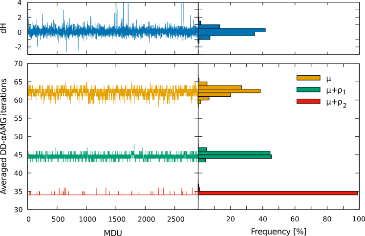
Figure 2: Top: The energy violation of the numerical integrator used during the MD of the $N_{f}=2$ ensemble plotted in units of MD trajectories (left) and its frequency (right). Bottom: DD-$\alpha$AMG iterations count averaged on MDU considering different monomials of the HMC simulation shown in units of MD trajectories (left) and its frequency (right). The results are for the $N_{f}=2$ ensemble listed in Table 1. The shifts $\rho_{i}$ are {0.0015, 0.015} and $\mu=0.000966$. The iterations count corresponds to average of the sum of the count of the outer level during the calculation of the force in the MD.

In the $N_{f}=2$ simulations we employ the Hasenbusch mass preconditioning Hasenbusch:2002ai by introducing additional mass terms and split up the determinants into additional ratios as in the following

$$\det\left[Q^{2}+\mu^{2}\right]=\det\left[\frac{Q^{2}+\mu^{2}}{Q^{2}+(\mu+\rho_{1})^{2}}\right]\det\left[\frac{Q^{2}+(\mu+\rho_{1})^{2}}{Q^{2}+(\mu+\rho_{2})^{2}}\right]\det\left[\frac{Q^{2}+(\mu+\rho_{2})^{2}}{Q^{2}+(\mu+\rho_{3})^{2}}\right]\det\left[Q^{2}+(\mu+\rho_{3})^{2}\right]$$ (3)

where $Q=\Gamma_{5}D=Q^{\dagger}$ is the hermitian Wilson Dirac operator. Each determinant in the right hand side (rhs) of Eq. 3 can be placed on a different monomial and integrated on a different time-scale. The time-steps are chosen accordingly to the intensity of the force term. This procedure controls the large fluctuations of the force terms, avoiding instabilities during the HMC.

In our $N_{f}=2$ simulation given in Table 1, we use 5 time-scales, which are integrated respectively $N_{\text{int}}=\{20,60,180,540,1620\}$ times. The gauge action is placed in the innermost time-scale; in the other time-scales we place one by one the fermionic determinants from the rhs of Eq. (3) going from the largest shift to the smallest. As depicted in Fig. 2, this yields a stable simulation without large spikes in the energy violation $\delta H$ with an acceptance rate of 84.5%. For the Hasenbusch mass preconditioning we use the shifts $\mu+\rho_{i}$ depicted in Fig. 1. The DD-$\alpha$AMG method is faster than CG solver for all the shifts except the largest given by $\rho_{3}$. Thus we have used DD-$\alpha$AMG for the inversions with shifts $\mu$, $\mu+\rho_{1}$ and $\mu+\rho_{2}$. The DD-$\alpha$AMG iterations count averaged per MD trajectory is depicted in Fig. 2. No exceptional fluctuations or correlations with larger energy violation $\delta H$ are seen along the simulation. The stability of the multigrid method is ensured by updating the setup every time the inversion at the physical quark mass, i.e. $(Q^{2}+\mu^{2})^{-1}$, is performed. The update is based on the previous setup by using one setup iteration, which is possible due to the adaptivity in the DD-$\alpha$AMG method Frommer:2013kla for the definition of the setup iteration. At the beginning of the trajectory we perform three setup iterations. The final speed-up, including setup costs, is a factor of 8 compared to CG in $N_{f}=2$ simulations at the physical pion mass.

3 $N_{f}=2+1+1$ multigrid accelerated (R)HMC simulations

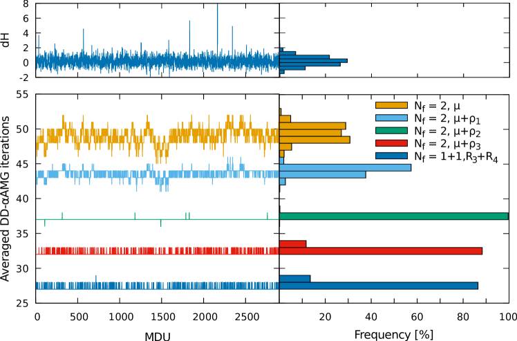
Figure 3: Top: The energy violation of the numerical integrator used during the MD of the $N_{f}=2+1+1$ ensemble plotted in units of MD trajectories (left) and its frequency (right). Bottom: DD-$\alpha$AMG iterations count averaged on MDU considering different monomials of the HMC simulation shown in units of MD trajectories (left) and its frequency (right). The results are for the $N_{f}=2+1+1$ ensemble listed in Table 1. The shifts $\rho_{i}$ are $\{0.0003,0.0012,0.01\}$ and $\mu=0.00072$. The monomials $\text{R}_{3}$ and $\text{R}_{4}$ contain the four smallest shifts of the rational approximation. The iterations count corresponds to average of the sum of the counts of the outer level during the calculation of the force in the MD.

In $N_{f}=2+1+1$ simulations we follow the same prescription reported in the previous section. Additionally to the determinants in the rhs of Eq. 3, the determinant of the non-degenerate $N_{f}=1+1$ TM operator $D_{\text{\scriptsize{ND}}}$ in Eq. (2) is included in the action. Monte Carlo algorithms require a positive weight, which can be retrieved for the non-hermitian operator $D_{\text{\scriptsize{ND}}}$ by using the Rational HMC (RHMC) Clark:2006fx . Here the determinant is rewritten as

$$\det\left[D_{\text{\scriptsize{ND}}}^{\phantom{-1}}(\bar{\mu},\bar{\epsilon})\right]=\det\left[\sqrt{Q_{\text{\scriptsize{ND}}}^{2}}\right]=\det\left[R^{-1}_{\text{\scriptsize{ND}}}\right]\det\left[\left|Q_{\text{\scriptsize{ND}}}^{\phantom{-1}}\right|R_{\text{\scriptsize{ND}}}^{\phantom{-1}}\right],$$ (4)

where $Q_{\text{\scriptsize{ND}}}^{\phantom{\dagger}}=(\Gamma_{5}\otimes\tau_{1})D_{\text{\scriptsize{ND}}}^{\phantom{\dagger}}=Q_{\text{\scriptsize{ND}}}^{\dagger}$ is the hermitian version of $D_{\text{\scriptsize{ND}}}$. The term $R_{\text{\scriptsize{ND}}}$ is the optimal rational approximation of

$$\frac{1}{\sqrt{Q_{\text{\scriptsize{ND}}}^{2}}}\simeq R_{\text{\scriptsize{ND}}}\equiv R_{n,\epsilon}\left(Q_{\text{\scriptsize{ND}}}^{2}\right)=a_{n,\epsilon}\prod_{i=1}^{n}\frac{Q_{\text{\scriptsize{ND}}}^{2}+c_{n,\epsilon,(2i-1)}I}{Q_{\text{\scriptsize{ND}}}^{2}+c_{n,\epsilon,2i}I},$$ (5)

where $n$ is the order of the approximation and $\epsilon=\lambda_{\min}/\lambda_{\max}$ is fixed by the smallest and largest eigenvalue of $Q_{\text{\scriptsize{ND}}}^{2}$, $\lambda_{\min}$ and $\lambda_{\max}$, respectively. The coefficients $a_{n,\epsilon}$ and $c_{n,\epsilon,i}$ are given by the Zolotarev solution for the optimal rational approximation zolotarev1877application . The rational approximation is optimal because the largest deviation from the approximated function is minimal according to the de-Vallée-Poussinâs theorem. In general, one can relax the approximation of the square root by introducing a correction term $\det\left[\left|Q_{\text{\scriptsize{ND}}}^{\phantom{-1}}\right|R_{\text{\scriptsize{ND}}}^{\phantom{-1}}\right]$ as in the rhs of Eq. (4). It takes into account the deviation from $\left|Q_{\text{\scriptsize{ND}}}\right|$ being close to the identity as much as the rational approximation is precise. For this reason we include it only in the acceptance step.

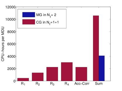
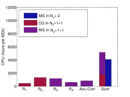
Figure 4: Costs per MDU of the $N_{f}=2+1+1$ simulation shown in units of CPU hours. In the left panel all the inversions in the RHMC are computed with a MMS-CG solver while in the right panel an hybrid approach of MMS-CG and DD-$\alpha$AMG solvers is used. The last column, “Sum”, reports the cost of RHMC in the $N_{f}=1+1$ sector compared to HMC in $N_{f}=2$ sector. The other columns regard different components of the RHMC: the “$\text{R}_{i}$”s are the rational approximation split in different monomial – $\text{R}_{1}$ contains the largest shifts while $\text{R}_{4}$ the smallest – and “Acc-Corr” is the cost for the acceptance and correction step.

In our $N_{f}=2+1+1$ simulation with properties given in Table 1, we use a rational approximation of order $n=10$, which has a relative deviation such that $\left\lVert\left|Q_{\text{\scriptsize{ND}}}\right|R_{\text{\scriptsize{ND}}}^{\phantom{-1}}\right\rVert_{\infty}<1.4\cdot 10^{-6}$, considering the eigenvalues of $Q_{\text{\scriptsize{ND}}}^{2}$ in the interval $\lambda_{\min}=6.5\cdot 10^{-5}$ and $\lambda_{\max}=4.7$. The product of ratios in the rhs of Eq. (5) is split in four monomials $R_{1-4}$. The first two contain three shifts, the second two contain two shifts. We use a 6 level nested minimal norm second order integration scheme with integration steps $N_{\text{int}}=\{12,36,108,324,972,2916\}$. The four monomials $R_{1-4}$ are placed one by one in the four outermost time-scales. As depicted in Fig. 3, this yields relative small energy violation during the MD integration and an acceptance rate of 76.8%. In the same figure we depict the iterations count for the inversions done with DD-$\alpha$AMG. The setup update is done on the second time-scale for the shift $\mu+\rho_{1}$, since it is still close to the light quark mass. In this case, we find slightly larger fluctuations in the iteration count of the outer level of the multigrid solver compared to the $N_{f}=2$ simulation shown in Fig. 2. Overall the simulation is stable and we find no correlation of the iteration count with larger energy violations $\delta H$.

The solutions computed by DD-$\alpha$AMG for the shifted linear systems in the monomials $R_{3}$ and $R_{4}$ are accelerated by providing an initial guess. Considering a Taylor expansion, we obtain

$$(Q_{\text{\scriptsize{ND}}}\pm i\delta)^{-1}\simeq Q_{\text{\scriptsize{ND}}}^{-1}\mp i\delta Q_{\text{\scriptsize{ND}}}^{-2}.$$ (6)

Thus we can use the inversions of the previously computed shift, i.e. $Q_{\text{\scriptsize{ND}}}^{-1}$ and $Q_{\text{\scriptsize{ND}}}^{-2}$, for constructing an appropriate initial guess for the next shift. This saves up to 30% of the inversion time.

The computational cost of each monomial per MD trajectory is depicted in Fig. 4. The standard approach depicted in the left panel involves the employment of multi-mass-shift CG (MMS-CG) for inverting all in once the shifted linear systems. In the right panel we have depicted the costs of the simulation accelerated by using the DD-$\alpha$AMG solver for the most ill-conditioned linear systems. We achieve a speed-up for the $N_{f}=1+1$ sector of a factor of 2 compare to a full eo-MMS-CG algorithm. The overall speed-up for $N_{f}=2+1+1$ simulation at the physical light, strange and charm quark mass is a factor of 5.

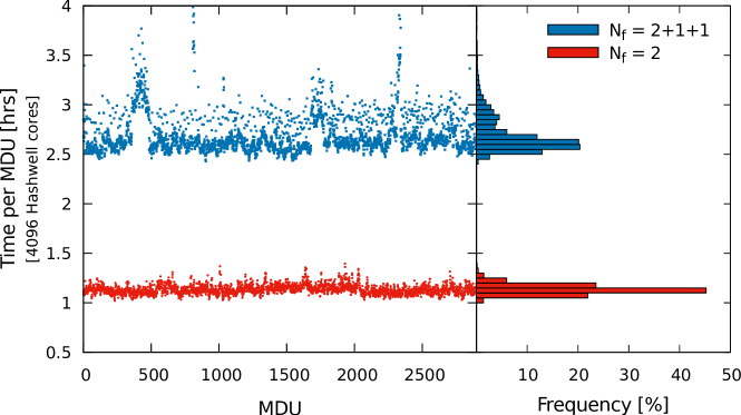
Figure 5: Time per MDU of the $N_{f}=2$ and $N_{f}=2+1+1$ ensembles in Table 1. The $N_{f}=2+1+1$ timings also include the calculation of the smallest and largest eigenvalue done at least every ten trajectories. The large fluctuation around MDU 500 for the $N_{f}=2+1+1$ ensemble is due to a bad allocation in the machine (it lasts exactly the duration of the allocation).

4 Conclusions

The multigrid accelerated simulations with TM fermions are discussed, showing a speed-up for simulations at the physical value of the pion mass of a factor of 8 in the case of $N_{f}=2$ and of a factor of $5$ in the case of $N_{f}=2+1+1$ compared to the simulations performed without multigrid. We use a three-level DD-$\alpha$AMG method optimized for TM fermions Alexandrou:2016izb . No instabilities in the iterations count are seen along the whole simulations. As depicted in Fig. 5, the time per MDU is quite stable with fluctuations within the 10%. During the $N_{f}=2+1+1$ simulation we calculate the smallest and largest eigenvalue of the non-degenerated TM operator at least every ten MDUs, which takes additionally 15 mins. This explains the single points that are frequently out of the main distribution. The two longer fluctuations instead are due to machine instabilities since they are limited to a single allocation of the job. Although the multigrid method is limiting significantly the parallelization of the calculation, the speed-up achieved makes feasible to sample enough MD trajectory. Indeed, the average time per MDU in the $N_{f}=2$ simulation is slightly larger than an hour and in the $N_{f}=2+1+1$ simulation below three hours. In both cases, 4096 cores employing 147 Haswell-nodes on SuperMUC are used. Indeed, we find that the three-level DD-$\alpha$AMG method shows an almost ideal scaling up to this number of cores for a lattice with volume $V=64^{3}\times 128$.

Acknowledgments

This project has received funding from the Horizon 2020 research and innovation program of the European Commission under the Marie Sklodowska-Curie grant agreement No 642069. S.B. is supported by this program. This project has also received founding from PRACE Fourth Implementation Phase (PRACE-4IP) program of the European Commission under grant agreement No 653838. We would like to thank P. Dimopoulos, R. Frezzotti, B. Kostrzewa and C. Urbach for fruitful discussions during the generation of the ensembles. The authors gratefully acknowledge the Gauss Centre for Supercomputing under project number pr74yo for providing computing time on the GCS Supercomputer SuperMUC at Leibniz Supercomputing Centre.

References

- (1) R. Babich, J. Brannick, R.C. Brower, M.A. Clark, T.A. Manteuffel, S.F. McCormick, J.C. Osborn, C. Rebbi, Phys. Rev. Lett. 105, 201602 (2010), 1005.3043
- (2) A. Frommer, K. Kahl, S. Krieg, B. Leder, M. Rottmann, SIAM J. Sci. Comput. 36, A1581 (2014), 1303.1377
- (3) C. Alexandrou, S. Bacchio, J. Finkenrath, A. Frommer, K. Kahl, M. Rottmann, Phys. Rev. D94, 114509 (2016), 1610.02370
- (4) M.A. Clark, B. JoÃ, A. Strelchenko, M. Cheng, A. Gambhir, R. Brower (2016), 1612.07873
- (5) R. Frezzotti, G.C. Rossi, JHEP 08, 007 (2004), hep-lat/0306014
- (6) S. Bacchio, C. Alexandrou, J. Finkenrath, A. Frommer, K. Kahl, M. Rottmann, PoS LATTICE2016, 259 (2016), 1611.01034
- (7) J. Finkenrath, C. Alexandrou, S. Bacchio, P. Charalambous, P. Dimopoulos, R. Frezzotti, K. Jansen, B. Kostrzewa, C. Urbach, LATTICE2017 (2017)
- (8) M. Lüscher, Comput. Phys. Commun. 156, 209 (2004), hep-lat/0310048
- (9) M. Lüscher, JHEP 07, 081 (2007), 0706.2298
- (10) K. Jansen, C. Urbach, Comput. Phys. Commun. 180, 2717 (2009), 0905.3331
- (11) I. Omelyan, I. Mryglod, R. Folk, Computer Physics Communications 151, 272 (2003)
- (12) A. Abdel-Rehim et al. (ETM), Phys. Rev. D95, 094515 (2017), 1507.05068
- (13) M. Hasenbusch, K. Jansen, Nucl. Phys. B659, 299 (2003), hep-lat/0211042
- (14) A. Frommer, K. Kahl, S. Krieg, B. Leder, M. Rottmann (2013), 1307.6101
- (15) M.A. Clark, A.D. Kennedy, Phys. Rev. Lett. 98, 051601 (2007), hep-lat/0608015
- (16) E. Zolotarev, Zap. Imp. Akad. Nauk. St. Petersburg 30, 1 (1877)