A New Coherence-Penalized Minimal Path Model with Application to Retinal Vessel Centerline Delineation

Abstract

In this paper, we propose a new minimal path model for minimally interactive retinal vessel centerline extraction. The main contribution lies at the construction of a novel coherence-penalized Riemannian metric in a lifted space, dependently of the local geometry of tubularity and an external scalar-valued reference feature map. The globally minimizing curves associated to the proposed metric favour to pass through a set of retinal vessel segments with low variations of the feature map, thus can avoid the short branches combination problem and shortcut problem, commonly suffered by the existing minimal path models in the application of retinal imaging. We validate our model on a series of retinal vessel patches obtained from the DRIVE and IOSTAR datasets, showing that our model indeed get promising results.

Index Terms—  Retinal Vessel Extraction, Minimal Path, Fast Marching Method, Feature Coherence.

1 Introduction

The minimal path model is a powerful tool for vessel centerline delineation thanks to its numerical efficiency, global optimality and elegant mathematical background. In the original formulation [1], a vessel can be modelled as a globally minimizing curve dependent of a metric, through which the minimal paths can be obtained through the solution to the respective Eikonal partial differential equation (PDE) by the fast marching methods [2, 3].

The classical Cohen-Kimmel model [1] provides a general Eikonal PDE framework for vessel segmentation. One research line on the improvements of the Cohen-Kimmel model is to design proper metrics to address different situations. In practice, it is interesting to take into account the orientations which a vessel should have for minimal path enhancement. This can be done by invoking anisotropic Riemannian metrics [4] or orientation lifted isotropic metrics [5] for geodesic distance computation. In order to obtain a smooth minimal path, the sub-Riemannian metric [6] and the Finsler elastica metric [7] were developed in an orientation space based on the Eikonal PDE framework, which in some extent can find solutions for artery extraction, but also suffer from the short branches combination problem especially when extracting a long artery. Other interesting shortest path models include [8, 9, 10].

In this paper, we propose a coherence-penalized minimal path model, where the associated minimal paths favour to pass by a vessel that is located in the flatten region of an external feature map. We observe that along a piece of retinal vessel, the values of gray levels vary slowly. More specifically, retinal arteries have lower contrast of gray levels than veins due to the blood materials and imaging modality. In other words, in some extent the arteries and veins are distinguishable in terms of vesselness values. Such an observation can be used to solve the short branches problem that the minimal paths associated to a metric may pass through segments belonging to different vessels as shown in Figs. 1b and 1c. Fig. 1d shows the result from the proposed method, which can avoid such problem. Fig. 1a gives the artery-vein (AV) groundtruth. In this paper, we denote by blue and green dots the source and end points respectively.

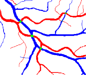
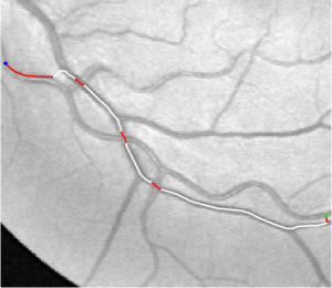
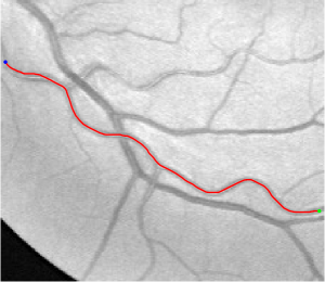
Fig. 1: Short branches combination. Column 1 Red, blue and green regions respectively indicate arteries, veins and their overlaps. Columns 2-3 Results from [4] and our method.

2 Background on Riemannian Geodesics

Definition 1

Let $\Omega\subset\mathbb{R}^{d}$ be an open bounded domain with $d$ the dimension and let $S^{+}_{d}$ be the set of positive symmetric definite (PSD) matrices. We denote by $\operatorname{Lips}([0,1],\Omega)$ the set of all Lipschitz paths $\eta:[0,1]\to\Omega$.

Definition 2

A Riemannian metric $\mathcal{P}:\Omega\times\mathbb{R}^{d}\to[0,\infty]$ is a convex function such that

$$\mathcal{P}(x,\mathbf{u}):=\sqrt{\langle\mathbf{u},\mathcal{M}(x)\,\mathbf{u}\rangle}=\|\mathbf{u}\|_{\mathcal{M}(x)},$$ (1)

where $\langle\cdot,\cdot\rangle$ denotes the Euclidean scalar product on $\mathbb{R}^{d}$ and $\mathcal{M}:\Omega\to S^{+}_{d}$ is a tensor field.

A Riemannian geodesic is a curve that globally minimizes a geodesic energy $\ell:\operatorname{Lips}([0,1],\Omega)\to[0,\infty]$ associated to a Riemannian metric $\mathcal{P}$

$$\ell(\eta)=\int_{0}^{1}\mathcal{P}\big{(}\eta(t),\dot{\eta}(t)\big{)}dt=\int_{0}^{1}\sqrt{\langle\dot{\eta}(t),\mathcal{M}(\eta(t))\,\dot{\eta}(t)\rangle}dt,$$

where $\eta\in\operatorname{Lips}([0,1],\Omega)$ and $\dot{\eta}$ denotes the first-order derivative of $\eta$. The tensor field $\mathcal{M}$ can be decomposed by its eigenvalues $\xi_{n}$ and eigenvectors $\mathfrak{q}_{n}$ such that

$$\mathcal{M}(x):=\sum_{n}\xi_{n}(x)\mathfrak{q}_{n}(x)\mathfrak{q}_{n}^{\rm T}(x).$$ (2)

For a source point $s$, the global minimum of $\ell$ between any point $x\in\Omega$ can be characterized by the minimal action map

$$\mathcal{U}_{s}(x):=\inf\,\{\ell(\eta);\eta\in\operatorname{Lips}([0,1],\Omega),\eta(0)=s,\eta(1)=x\},$$

which is the unique viscosity solution to the Eikonal PDE

$$\|\nabla\mathcal{U}(x)\|_{\mathcal{M}^{-1}(x)}=1,\,\forall x\in\Omega\setminus\{s\},~{}\text{and}\quad\mathcal{U}_{s}(s)=0.$$ (3)

The geodesic $\mathcal{C}_{\mathtt{s},\mathtt{x}}\in\operatorname{Lips}([0,1],\Omega)$ linking from $s$ to $x$ can be computed by re-parameterizing and reversing the geodesic $\rho_{\mathtt{x},\mathtt{s}}$ by solving the ordinary differential equation (ODE)

$$\begin{cases}&\rho_{\mathtt{x},\mathtt{s}}(t)=-\frac{\mathcal{M}^{-1}(\dot{\rho}_{\mathtt{x},\mathtt{s}}(t))\,\nabla\mathcal{U}(\rho_{\mathtt{x},\mathtt{s}}(t))}{\|\mathcal{M}^{-1}(\dot{\rho}_{\mathtt{x},\mathtt{s}}(t))\,\nabla\mathcal{U}(\rho_{\mathtt{x},\mathtt{s}}(t))\|},\\ &\rho_{\mathtt{x},\mathtt{s}}(0)=x.\end{cases}$$ (4)

For the task of retinal vessel centerline extraction, the tensor field $\mathcal{M}$ can be expressed by

$$\mathcal{M}(x)=\omega(x)\mathfrak{q}_{1}(x)\mathfrak{q}_{1}^{\rm T}(x)+\mathfrak{q}_{2}(x)\mathfrak{q}^{\rm T}_{2}(x),$$ (5)

where $\omega(x)=\exp\big{(}-\alpha P(x)\big{)}_{0}$ is a potential function with $\alpha\in\mathbb{R}^{+}$ and $P:\Omega\to[0,\infty)$ is a vesselness map which has large values around the vessel centerlines and low values in the background. It can be estimated by the tubularity filters such as [11, 12]. The vector $\mathfrak{q}_{1}(x)\in\mathbb{R}^{2}$ denotes an orientation that a vessel should have at point $x$ and $\mathfrak{q}_{2}(x)$ is orthogonal to $\mathfrak{q}_{1}(x)$.

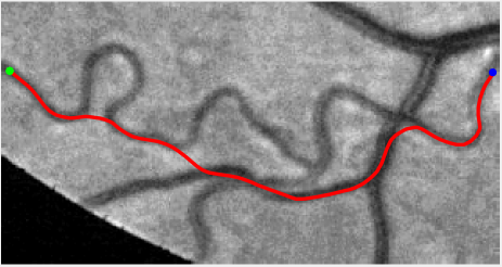
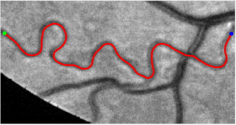
Fig. 2: Left Result by the curvature-penalized model [7]. Right Result from the proposed model after refinement step.

3 Coherence-Penalized Geodesic Model

In this section, we present a new coherence-penalized metric based on a scalar-valued smooth function $\mathcal{I}:\Omega\to\mathbb{I}\subset\mathbb{R}^{+}_{0}$.

3.1 Geodesic Energy with Coherence-penalized Metric

Let us consider a norm $\phi_{x}$ over $\mathbb{R}^{2}$ that depends on a directional derivative operator $\mathcal{D}_{\mathbf{u}}$ such that for any point $x\in\Omega$

$$\phi_{x}(\mathbf{u})=|\mathcal{D}_{\mathbf{u}}\mathcal{I}(x)|=\left|\lim_{\epsilon\to 0}\frac{\mathcal{I}(x+\epsilon\vec{u})-\mathcal{I}(x)}{\epsilon}\right|.$$ (6)

Therefore, one can point out that a small value of $\mathcal{D}_{\mathbf{u}}\mathcal{I}$ implies a low variation of $\mathcal{I}$ along the direction $\mathbf{u}$ at a point $x$. We consider a geodesic energy of a curve $\eta\in\operatorname{Lips}([0,1],\Omega)$

$$\mathcal{L}(\eta)=\int_{0}^{1}\sqrt{\|\dot{\eta}(t)\|_{\mathcal{M}(\eta(t))}+\beta\,\mathcal{H}^{2}(\eta(t),\dot{\eta}(t))}\,dt,$$ (7)

where the tensor field $\mathcal{M}$ is defined in Eq. (5) and $\beta\in\mathbb{R}^{+}_{0}$. The term $\mathcal{H}$ depends on the norm (6) such that

$$\mathcal{H}(x,\mathbf{u})=\omega(x)\phi_{x}^{2}(\mathbf{u})=\omega(x)|\langle\nabla\mathcal{I}(x),\mathbf{u}\rangle|^{2},$$ (8)

where the second equality is obtained by the reality $\mathcal{D}_{\mathbf{u}}\mathcal{I}(x)=\langle\nabla\mathcal{I}(x),\mathbf{u}\rangle$. The potential function is used in (5).

3.2 Minimizing $\mathcal{L}$ by a lifted metric approach

Definition 3

We define a space $\bar{\Omega}=\Omega\times\mathbb{I}\subset\mathbb{R}^{3}$ such that a point $\bar{x}=(x,\vartheta)\in\bar{\Omega}$ is a pair comprised of a spatial point $x\in\Omega$ and a position $\vartheta\in\mathbb{I}$.

Let $\tau:[0,\,1]\to\mathbb{I}$ be a differentiable parametric function which is defined in terms of $\mathcal{I}$ and a path $\eta\in\operatorname{Lips}([0,1],\Omega)$

$$\tau=\mathcal{I}\circ\eta,$$ (9)

based on which, one has for any $t\in[0,1]$

$$\dot{\tau}(t)=\frac{\partial\tau}{\partial t}(t)=\frac{\partial\mathcal{I}(\eta(t))}{\partial t}=\langle\nabla\mathcal{I}(\eta(t)),\,\dot{\eta}(t)\rangle.$$ (10)

Integrating Eqs. (8) and (10), for a curve $\eta$ we have

$$\mathcal{H}^{2}(\eta(t),\dot{\eta}(t))=\omega(\eta(t))|\dot{\tau}(t)|^{2}$$ (11)

Based on the relation (9), for each curve $\eta\in\operatorname{Lips}([0,1],\Omega)$ one can construct a lifting curve $\gamma\in\operatorname{Lips}([0,1],\bar{\Omega})$ such that

$$\gamma(t):=(\eta(t),\tau(t)),\quad\text{and}\quad\dot{\gamma}(t)=(\dot{\eta}(t),\dot{\tau}(t)).$$ (12)

Now we can reformulate the geodesic energy $\mathcal{L}$ in Eq. (7) by

$$\mathcal{L}(\eta) =\int_{0}^{1}\sqrt{\|\dot{\eta}(t)\|_{\mathcal{M}(\eta(t))}+\beta\,\omega(\eta(t))|\dot{\tau}(t)|^{2}}\,dt,$$

$$=\int_{0}^{1}\mathcal{R}^{\infty}(\gamma(t),\dot{\gamma}(t))~{}dt=\mathcal{L}^{\infty}(\gamma),$$ (13)

where $\mathcal{R}^{\infty}:\bar{\Omega}\times\mathbb{R}^{3}\to[0,\infty]$ is a degenerated Riemannian metric. It can be expressed for any $\bar{x}=(x,r)\in\bar{\Omega}$ and any vector $\bar{\mathbf{u}}\in\mathbb{R}^{3}$

$$\mathcal{R}^{\infty}(\bar{x},\bar{\mathbf{u}}):=\begin{cases}\|\bar{\mathbf{u}}\|_{\mathcal{T}(x,\vartheta)},\quad&\text{if}~{}\vartheta=\mathcal{I}(x),\\ \infty,&\text{otherwise},\end{cases}$$ (14)

where $\mathcal{T}:\bar{\Omega}\to S^{+}_{3}$ is a PSD tensor field

$$\mathcal{T}(x,\vartheta)=\begin{pmatrix}\bar{\mathcal{M}}(x,\vartheta),&\mathbf{0}\\ \mathbf{0},&\beta\bar{\omega}(x,\vartheta)\end{pmatrix},$$ (15)

with $\bar{\mathcal{M}}(x,\vartheta):=\mathcal{M}(x)$ and $\bar{\omega}(x,\vartheta):=\omega(x)$.

The goal is to minimize $\mathcal{L}^{\infty}$ in Eq. (13) by solving the respective Eikonal PDE. However, the metric $\mathcal{R}^{\infty}$ is too singular for finding the numerical solutions. We introduce a new Riemannian metric $\mathcal{R}^{\lambda}:\bar{\Omega}\times\mathbb{R}^{3}\to[0,\infty]$ based on a penalization parameter $\lambda\gg 0$ for any $\bar{x}=(x,\vartheta)$ and any $\bar{\mathbf{u}}\in\mathbb{R}^{3}$

$$\mathcal{R}^{\lambda}(\bar{x},\vec{u}):=\mathfrak{C}_{\lambda}\big{(}\vartheta,\mathcal{I}(x)\big{)}\,\|\vec{u}\|_{\mathcal{T}(\mathtt{x})},$$ (16)

where $\mathfrak{C}_{\lambda}:\mathbb{I}\times\mathbb{I}\to\mathbb{R}^{+}_{0}$ is a distance map defined by

$$\mathfrak{C}_{\lambda}(a,b)=\exp(\lambda\,|a-b|^{p}),\quad\forall a,~{}b\in\mathbb{I},$$ (17)

where we set $p=1$ through this paper.

For a given source point $\bar{s}\in\bar{\Omega}$, the minimal action map $\mathcal{U}^{\lambda}_{\bar{s}}$ associated to the metric $\mathcal{R}^{\lambda}$ can be estimated efficiently by the anisotropic fast marching method [3]. The geodesic $\bar{\mathcal{C}}_{\bar{\mathtt{s}},\bar{\mathtt{x}}}$ linking the source point $\bar{s}$ to a point $\bar{x}$ can be computed via the solution to the gradient descent ODE (4) on $\mathcal{U}_{\bar{s}}^{\lambda}$.

Minimal paths refinement processing. In practice, sometimes the resulting geodesics $\bar{\mathcal{C}}_{\bar{\mathtt{s}},\bar{\mathtt{x}}}$ by the metric $\mathcal{R}^{\lambda}$ do not exactly follow the real centerlines because of the local gray level inhomogeneities. Here we use the region-constrained minimal path model proposed in [13] to refine these geodesics.

Compare to existing minimal path models. The Riemannian metrics used in [1, 4, 5] are based on the local pointwise information. The curvature-penalized metric [7, 6] and the proposed coherence-penalized metric are able to consider more constraints, i.e., the rigidity for [7, 6] and feature coherence for our metric. These constraints are beneficial to the respective geodesics to reduce the risk of short branches combination problem. Compared to the curvature-penalized metric, our method can be more flexible since the feature map $\mathcal{I}$ can be produced dependently on the task. In retinal imaging, veins and arteries are distinguishable in terms of gray levels or vesselness values, satisfying the formulation of the proposed model. Especially for vessels with strong tortuosity, the curvature-penalized metric， which favours a smooth curve, fails to catch the expected vessels as shown in the left column of Fig. 2. From the right column of Fig. 2, one can see that our model can obtain a good result.

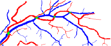
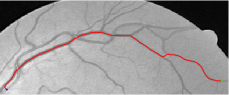
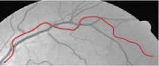
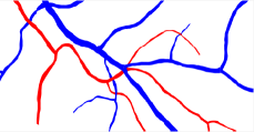
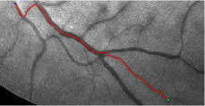
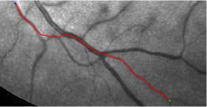
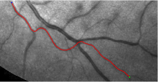
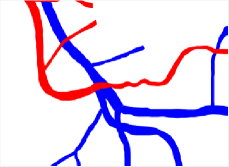
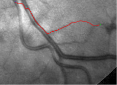
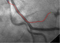
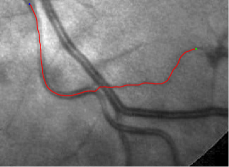
Fig. 3: Column1 shows the AV groundtruth. Columns 2-4 are paths from the ArR, CuP and the proposed models respectively.

4 Experimental Results

Computation of the local vessel geometry. There exist a series of methods [11, 12] for local vessel geometry computation, among which we choose the optimally oriented flux filter (OOF) [12] as our feature extractor. The multi-scale outputs of the OOF can be expressed as $\mathbf{Q}(x,r)=\left(\frac{1}{r}(\partial_{ij}G_{\sigma})_{ij}\ast\mathbbm{1}_{r}\ast I\right)(x)$, where $\mathbbm{1}_{r}$ is a step function centred at point $x$ with scale $r$ and $(\partial_{ij}G_{\sigma})_{ij}$ is the Hessian matrix of the Gaussian kernel $G_{\sigma}$ with variance $\sigma$. Generally, we can assume that the gray levels inside the vessels are lower than background and $\xi_{1}\leq\xi_{2}$. By decomposing $\mathbf{Q}$ by its eigenvalues $\hat{\xi}_{n}$ and eigenvectors $\hat{\mathfrak{q}}_{n}$, we can define an optimal scale map $\mathcal{S}(x)=\arg\min_{r}\hat{\xi}_{2}(x,r)$. The vesselness map $P$ can be computed by $P(x)=\max\{0,~{}\xi_{2}(x,\mathcal{S}(x))\}$. The eigenvectors $\mathfrak{q}_{n}$ of $\mathcal{M}$ in Eq. (5) can be defined as $\mathfrak{q}_{n}(x)=\hat{\mathfrak{q}}_{n}(x,\mathcal{S}(x))$. The feature map $\mathcal{I}$ is constructed via a smoothed vesselness map $\tilde{P}:=F\ast P$ where $F$ is a mean filter or a Gaussian filter. The interval $\mathbb{I}=[0,\|\mathcal{I}\|_{\infty}]$ is discretized evenly to $120$ levels in all the experiments.

Validation. We validate our minimal path model on respective 54 and 30 patches obtained from the DRIVE [14, 15] and the IOSTAR [16] datasets with AV groundtruth. Each artery involved in these parches locates near a vein or crossing it at least once. Our goal is to extract the artery between two given points. In order to get the quantitative evaluation, we first convert each continuous spatial path $\mathcal{C}$ to an 4-connected digital path $\Gamma\subset\Omega$ which is considered as a pixel collection. We denote by $\chi=\{x\in\Gamma\cap A\}$ the collection of digital path pixels inside the artery groundtruth map $A$. Thus, a measure $\Theta$ can be simply defined as $\Theta=|\chi|/|\Gamma|$, where $|\chi|$ and $|\Gamma|$ mean the respective number of elements involved in $\chi$ and $\Gamma$. We compare our model to four existing minimal path models: the isotropic Riemannian (IR) model [1], the anisotropic radius-lifted Riemannian (ArR) model [4], the isotropic orientation-lifted Riemannian (IoR) model [5] and the curvature-penalized (CuP) model [7]. The construction of these metrics are based on the OOF outputs [12]. Note that a centerline-based potential is chosen so that we remove the radius dimension of [5] to reduce computation complexity. The results in terms of the $\Theta$ score are presented in Table 1, including the average (Avg.), maximum (Max.), minimum (Min.) and standard deviation (Std.) values. In both DRIVE and IOSTAR datasets, our method can achieve the best performances thanks to the coherence penalization. Note that in Table 1, we evaluate our method by using the refined paths instead of using the original coherence-penalized minimal paths. For comparisons in visualization, we show the minimal paths from the ArR metric , the CuP metric and the proposed coherence-penalized metric on three retinal patches as shown in Fig. 3. The targeted artery vessels which cross veins at least once are labeled by red color in column 1. The paths shown in column 4 from the proposed metric are results after refinement. One can claim that our method indeed can catch expected arteries while other metrics fall into the traps of short branches combination.

Table 1: Quantitative comparisons of different metrics.

$\Theta~{}\quad$		IR	ArR	IoR	CuP	Proposed
DRIVE	Avg.	0.39	0.39	0.34	0.65	0.98
	Max.	1.0	1.0	1.0	1.0	1.0
	Min.	0.03	0.02	0.02	0.13	0.83
	Std.	0.22	0.28	0.28	0.28	0.04
IOSTAR	Avg.	0.44	0.48	0.48	0.70	0.90
	Max.	0.98	0.98	0.97	0.97	0.99
	Min.	0.02	0.03	0.03	0.06	0.63
	Std.	0.30	0.32	0.32	0.30	0.08

5 Conclusion

In this paper, we propose a new metric invoking a coherence penalty on the variation of an external feature map along the geodesics for minimally interactive retinal vessel segmentation. We interpret the geodesic energy with a coherence penalty through a coherence-penalized metric. In order to compute the associated geodesics by fast marching method, we use an approximation of such a coherence-penalized metric. Experimental results show that our model indeed obtain promising results in retinal vessel segmentation.

References

- [1] L. D. Cohen and Ron Kimmel, “Global minimum for active contour models: A minimal path approach,” IJCV, vol. 24, no. 1, pp. 57–78, 1997.
- [2] James A Sethian, “Fast marching methods,” SIAM review, vol. 41, no. 2, pp. 199–235, 1999.
- [3] J-M Mirebeau, “Anisotropic fast-marching on cartesian grids using lattice basis reduction,” SINUM, vol. 52, no. 4, pp. 1573–1599, 2014.
- [4] F. Benmansour and L. D. Cohen, “Tubular structure segmentation based on minimal path method and anisotropic enhancement,” IJCV, vol. 92, no. 2, pp. 192–210, 2011.
- [5] M. Péchaud, R. Keriven, and G. Peyré, “Extraction of tubular structures over an orientation domain,” in CVPR, 2009, pp. 336–342.
- [6] E. J Bekkers et al., “A PDE approach to data-driven sub-riemannian geodesics in SE (2),” SIIMS, vol. 8, no. 4, pp. 2740–2770, 2015.
- [7] D. Chen, J-M Mirebeau, and L.D Cohen, “Global minimum for a Finsler elastica minimal path approach,” IJCV, vol. 122, no. 3, pp. 458–483, 2017.
- [8] W. Liao et al., “Progressive minimal path method for segmentation of 2D and 3D line structures,” TPAMI, 2017.
- [9] Lu Wang, Vinutha Kallem, et al., “Interactive retinal vessel extraction by integrating vessel tracing and graph search,” in MICCAI, 2013, pp. 567–574.
- [10] J. Ulén et al., “Shortest paths with higher-order regularization,” TPAMI, vol. 37, no. 12, pp. 2588–2600, 2015.
- [11] A. F Frangi, W. J Niessen, K. L Vincken, and M. A Viergever, “Multiscale vessel enhancement filtering,” in MICCAI, 1998, pp. 130–137.
- [12] M. WK Law and A. CS Chung, “Three dimensional curvilinear structure detection using optimally oriented flux,” in ECCV, 2008, pp. 368–382.
- [13] D. Chen and L. D Cohen, “Piecewise geodesics for vessel centerline extraction and boundary delineation with application to retina segmentation,” in SSVM, 2015, pp. 270–281.
- [14] J. Staal et al., “Ridge-based vessel segmentation in color images of the retina,” TMI, vol. 23, no. 4, pp. 501–509, 2004.
- [15] Q. Hu et al., “Automated separation of binary overlapping trees in low-contrast color retinal images,” in MICCAI, 2013, pp. 436–443.
- [16] J. Zhang et al., “Robust retinal vessel segmentation via locally adaptive derivative frames in orientation scores,” TMI, vol. 35, no. 12, pp. 2631–2644, 2016.