Strong Consistency of Spectral Clustering for Stochastic Block Models

Abstract

In this paper we prove the strong consistency of several methods based on the spectral clustering techniques that are widely used to study the community detection problem in stochastic block models (SBMs). We show that under some weak conditions on the minimal degree, the number of communities, and the eigenvalues of the probability block matrix, the K-means algorithm applied to the eigenvectors of the graph Laplacian associated with its first few largest eigenvalues can classify all individuals into the true community uniformly correctly almost surely. Extensions to both regularized spectral clustering and degree-corrected SBMs are also considered. We illustrate the performance of different methods on simulated networks.

Key words and phrases: Community detection, degree-corrected stochastic block model, K-means, regularization, strong consistency.

Abstract

This supplement is composed of four parts. Sections A and B provide the proofs of the main results in Sections 2 and 3, respectively. Section C contains some lemmas that are used in the proofs of the main results. Section D presents some additional simulation results.

Key words and phrases: Community detection, degree-corrected stochastic block model, K-means, regularization, strong consistency.

1 Introduction

Community detection is one of the fundamental problems in network analysis, where communities are groups of nodes that are, in some sense, more similar to each other than to the other nodes. The stochastic block model (SBM) that was first proposed by Holland et al. (1983) is a common tool for model-based community detection that has been widely studied in the statistics literature. Within the SBM framework, the most essential task is to recover the community membership of the nodes from a single observation of the network. Various procedures have been proposed to solve this problem in the last decade or so. These include method of moments (Bickel et al., 2011), modularity maximization (Newman and Girvan, 2004), semidefinite programming (Abbe et al., 2016; Cai and Li, 2015), spectral clustering (Joseph and Yu, 2016; Lei and Rinaldo, 2015; Qin and Rohe, 2013; Rohe et al., 2011; Sarkar and Bickel, 2015; Vu, 2018; Yun and Proutiere, 2014, 2016), likelihood methods (Amini et al., 2013; Bickel and Chen, 2009; Choi et al., 2012; Zhao et al., 2012), and spectral embedding (Lyzinski et al., 2014; Sussman et al., 2012). Abbe (2018) provides an excellent survey on recent developments on community detection and stochastic block models. Among the methods mentioned above, spectral clustering is arguably one of the most widely used methods due to its computational tractability.

Bickel and Chen (2009) introduce the notion of strong consistency of community detection as the number of nodes, $n,$ grows. By strong consistency, they mean that one can identify the members of the block model communities perfectly in large samples. Based on the parameters of the block model, properties of the modularities, and expected degree of the graph ($\lambda_{n}$), Bickel and Chen (2009) give the sufficient conditions for strong consistency, which is $\lambda_{n}/\log(n)\rightarrow\infty.$ Zhao et al. (2012) define weak consistency of community detection, which essentially means that the number of misclassified nodes is of smaller order than the number of nodes. Bickel and Chen (2012) find that weak consistency requires that $\lambda_{n}\rightarrow\infty$ for the SBM. Similarly, under the conditions that $\lambda_{n}/\log(n)\rightarrow\infty$ ($\lambda_{n}\rightarrow\infty)$, Zhao et al. (2012) establish the strong (weak) consistency under both standard SBMs and degree-corrected SBMs.

If the community detection method is strongly consistent, then it means that the communities are exactly recoverable. From an information-theory perspective, Abbe and Sandon (2015), Abbe et al. (2016), Mossel et al. (2014), and Vu (2018) study the phase transition threshold for exact recovery, which requires $\lambda_{n}=\Omega(\log(n))$. It is well known that some methods like the modularity maximization of Newman and Girvan (2004) and the likelihood method of Bickel and Chen (2009) yield strongly consistent community recovery, but they either rely on combinatorial methods that are computationally demanding or are guaranteed to be successful only when the starting values are well-chosen. Abbe et al. (2016) show that semidefinite programming can achieve exact recovery when there are two equal-sized communities. Yun and Proutiere (2014), Yun and Proutiere (2016), and Vu (2018) establish strong consistency for the variants of spectral method, which involve graph splitting, trimming, and a final improvement step. The pure spectral clustering method has been shown to enjoy weak consistency under standard or degree-corrected SBMs by various researchers; see Joseph and Yu (2016), Lei and Rinaldo (2015), Qin and Rohe (2013), and Rohe et al. (2011). Weak consistency here means that the fraction of misclassified nodes decreases to zero as $n$ grows. Because the decrease rates established in above papers are usually slower than $n$, the above weak consistency results imply that the number of misclassified nodes still increases to infinity as $n$ grows. On the contrary, strong consistency implies that the number of misclassified nodes is zero for sufficiently large $n$, which greatly improves upon weak consistency.

The aim of this paper is to formally establish the strong consistency of spectral clustering for standard/regular SBMs without any extra refinement steps, under a set of conditions on the minimal degree of nodes ($\mu_{n}$), the number of communities ($K$), the minimal value of the nonzero eigenvalue of the normalized block probability matrix, and some other parameters of the block model. In the special case where $K$ is fixed and the normalized block probability matrix has minimal eigenvalue bounded away from zero in absolute value, we show that $\mu_{n}/\log(n)$ being sufficiently large can ensure strong consistency. In other words, the spectral clustering method achieves the optimal rate for exact recovery, as pointed out in Abbe et al. (2016) and Abbe and Sandon (2015).

As demonstrated by Amini et al. (2013), the performance of spectral clustering can be considerably improved via regularization. Joseph and Yu (2016) provide an attempt at quantifying this improvement through theoretical analysis and find that the typical minimal degree assumption for the consistency of spectral clustering can potentially be removed with suitable regularization. In this paper, we also establish the strong consistency of regularized spectral clustering.

The SBM is limited by its assumption that all nodes within a community are stochastically equivalent and thus provides a poor fit to real-world networks with hubs or highly varying node degrees within communities. For this reason, Karrer and Newman (2011) propose a degree-corrected SBM (DC-SBM) to allow variation in node degrees within a community while preserving the overall block community structure. The DC-SBM greatly enhances the flexibility of modeling degree heterogeneity and enables us to fit network data with varying degree distributions. We also prove the strong consistency of spectral clustering for regularized DC-SBMs.

Our paper is mostly related to Abbe et al. (2017). Abbe et al. (2017) derive the $L_{\infty}$ bound for the entrywise eigenvector of random matrices with low expected rank. Then they apply their general results to SBM with two communities, where both within- and cross-community probabilities are of order $\log(n)/n$ and show that classifying nodes based on the sign of the entries in the second eigenvector can achieve exact recovery. Our paper complements theirs in the following three aspects. First, we consider the eigenvectors of normalized graph Laplacian $L$ rather than the adjacency matrix $A$. Therefore, the entrywise bound of the eigenvectors derived in Abbe et al. (2017) cannot be directly used in our case. Our proof relies on the construction of a contraction mapping for the entrywise bound, via which we can iteratively refine the bound. Such strategy is different from that in Abbe et al. (2017).

Second, we consider SBM with a general block probability matrix whereas Abbe et al. (2017) consider a $2\times 2$ block probability matrix. Even though Abbe et al. (2017) establish general theories of $L_{\infty}$ bound for the entrywise eigenvector of random matrices, when applying their theory to SBMs, they only study the model with the following block probability matrix:

$$\begin{pmatrix}\frac{a\log(n)}{n}&\frac{b\log(n)}{n}\\ \frac{b\log(n)}{n}&\frac{a\log(n)}{n}\end{pmatrix}.$$ (1.1)

Their block probability matrix assumes that there are two groups, the connection probability within groups are the same for the two groups, and the within- and cross-group connection probabilities are of the same order of $\log(n)/n$. In contrast, our paper studies the general SBM with generic $K$ groups, where $K$ is allowed to diverge to infinity at a slow rate and the decay rates for different elements in the block probability matrix can be different. When there are two communities, Abbe et al. (2017) use the sign of the eigenvector associated with the second largest eigenvalue (in absolute value) to identify the node’s membership. When $K>2$, just checking the sign is not sufficient to identify all $K$ groups. Our paper shows that applying the K-means algorithm to the first $K$ eigenvectors can achieve strong consistency.

Third, we consider SBM with both regularization and degree correction. We show that, by regularization, the strong consistency is still possible even when the minimal degree does not diverge at all. For the DC-SBM with regularization, we also derive the conditions for strong consistency. Neither regularization nor degree-corrected SBM is discussed in Abbe et al. (2017).

In the simulation, we consider both standard SBMs and DC-SBMs. For standard SBMs, we adopt Joseph and Yu (2016)’s regularization method and choose the tuning parameter $\tau$ according to their recommendation. The results show that in terms of classification, spectral clustering tends to outperform the unconditional pseudo-likelihood (UPL) method, which also has the strong consistency property (Amini et al., 2013). In contrast, for the DC-SBMs our simulations suggest that the regularized spectral clustering tends to slightly underperform the conditional pseudo-likelihood (CPL) method even though both are strongly consistent under some conditions. We also show that an adaptive procedure helps the regularized spectral clustering to achieve much better performance than the CPL method.

The rest of the paper is organized as follows. We study the strong consistency of spectral clustering for the basic SBMs in Section 2. We consider the extensions to regularized spectral clustering and degree-corrected SBMs in Section 3. Section 4 reports the numerical performance of various spectral-clustering-based methods for a range of simulated networks. Section 5 describes the proof strategy of the key theorem in our paper. Section 6 concludes. The proofs of the main results are relegated to the mathematical appendix.

Notation. Throughout the paper, we use $[M]_{ij}$ and $[M]_{i\cdot}$ to denote the $(i,j)$-th entry and $i$-th row of matrix $M$, respectively. Without confusion, we sometimes simplify $[M]_{ij}$ as $M_{ij}$. $\|M\|$ and $\|M\|_{F}$ denote the spectral norm and Frobenius norm of $M,$ respectively. Note that $\|M\|=\|M\|_{F}$ when $M$ is a vector. In addition, let $\|M\|_{2\rightarrow\infty}=\sup_{i}\|[M]_{i\cdot}\|.$ We use $\mathbf{1}\left\{\cdot\right\}$ to denote the indicator function which takes value 1 when $\cdot$ holds and 0 otherwise. $C_{1}$ and $c_{1}$ denote specific absolute constants that remain the same throughout the paper.

2 Strong consistency of spectral clustering

2.1 Basic setup

Let $A\in\{0,1\}^{n\times n}$ be the adjacency matrix. By convention, we do not allow self-connection, i.e., $A_{ii}=0$. Let $\hat{d}_{i}=\sum_{j=1}^{n}A_{ij}$ denote the degree of node $i$, $D=\text{diag}(\hat{d}_{1},\ldots,\hat{d}_{n})$, and $L=D^{-1/2}AD^{-1/2}$ be the graph Laplacian. The graph is generated from a SBM with $K$ communities. We assume that $K$ is known and potentially depends on the number of nodes $n$. We omit the dependence of $K$ on $n$ for notation simplicity. If $K$ is unknown, it can be determined by either Lei’s 2016 sequential goodness-of-fit testing procedure, the likelihood-based model selection method proposed by Wang and Bickel (2017), or the network cross-validation method proposed by Chen and Lei (2017). The communities, which represent a partition of the $n$ nodes, are assumed to be fixed beforehand. Denote these by $C_{1},\ldots,C_{K}$. Let $n_{k}$, for $k=1,\ldots,K$, be the number of nodes belonging to each of the clusters.

Given the communities, the edge between nodes $i$ and $j$ are chosen independently with probability depending on the communities $i$ and $j$ belong to. In particular, for nodes $i$ and $j$ belonging to cluster $C_{k_{1}}$ and $C_{k_{2}}$, respectively, the probability of edge between $i$ and $j$ is given by $P_{ij}=B_{k_{1}k_{2}}$, where the block probability matrix $B=\{B_{k_{1}k_{2}}\}$, $k_{1},k_{2}=1,\ldots,K$, is a symmetric matrix with each entry between $[0,1]$. The $n\times n$ edge probability matrix $P=\{P_{ij}\}$ represents the population counterpart of the adjacency matrix $A$. Frequently we suppress the dependence of matrices and their elements on $n.$

Denote $Z=\{Z_{ik}\}$ as the $n\times K$ binary matrix providing the cluster membership of each node, i.e., $Z_{ik}=1$ if node $i$ is in $C_{k}$ and $Z_{ik}=0$ otherwise. Then we have $P=ZBZ^{T}.$ Let $\mathcal{D}=\text{diag}(d_{1},\ldots,d_{n})$ where $d_{i}=\sum_{j=1}^{n}P_{ij}$. The population version of the graph Laplacian is $\mathcal{L}=\mathcal{D}^{-1/2}P\mathcal{D}^{-1/2}.$ The standard spectral clustering corresponds to classifying the eigenvectors of $L$ by K-means algorithm. In this paper, we focus on the strong consistency of both the standard spectral clustering and its variant.

2.2 Identification of the group membership

Let $\pi_{kn}=n_{k}/n$, $W_{k}=[B]_{k\cdot}Z^{T}\iota_{n}/n=\sum_{l=1}^{K}B_{kl}\pi_{ln}$, $\mathcal{D}_{B}=\text{diag}(W_{1},\ldots,W_{K})$, and $B_{0}=\mathcal{D}_{B}^{-1/2}B\mathcal{D}_{B}^{-1/2}$, where $\iota_{n}$ is a vector of ones in $\Re^{n}$. We can view $W_{k}$ as the weighted average of the $k$-th row of $B$ with weights given by $\pi_{kn}.$ Similarly, $B_{0}$ is a normalized version of $B$. Note that $B_{0}$ is symmetric as $B$ is. Let $\Pi_{n}=\text{diag}(\pi_{1n},\ldots,\pi_{Kn})$. Throughout the paper, we allow for the elements in the block probability matrix $B$ to depend on $n$ and decay to zero as $n$ grows, which leads to a sparse graph.

Assumption 1.

$B_{0}$ has rank $K$ and the spectral decomposition of $\Pi_{n}^{1/2}B_{0}\Pi_{n}^{1/2}$ is $S_{n}\Omega_{n}S_{n}^{T}$, in which $S_{n}$ is a $K\times K$ matrix such that $S_{n}^{T}S_{n}=I_{K}$ and $\Omega_{n}=\text{diag}(\omega_{1n},\ldots,\omega_{Kn})$ such that $|\omega_{1n}|\geq\cdots\geq|\omega_{Kn}|>0$.

Assumption 1 implies that $B=\mathcal{D}_{B}^{1/2}\Pi_{n}^{-1/2}S_{n}\Omega_{n}S_{n}^{T}\Pi_{n}^{-1/2}\mathcal{D}_{B}^{1/2}$ and $B_{0}=\Pi_{n}^{-1/2}S_{n}\Omega_{n}S_{n}^{T}\Pi_{n}^{-1/2}$. The full-rank assumption is also made in Rohe et al. (2011), Lei and Rinaldo (2015), and Joseph and Yu (2016) and can be relaxed at the cost of more complicated notation. In addition, we allows for the possibility that $K\rightarrow\infty$ and/or $\omega_{Kn}\rightarrow 0$ as $n\rightarrow\infty$ below. This also mitigates concern of the full-rank condition. Assumption 1 implies that $\mathcal{L}$ has rank $K$ and the following spectral decomposition:

$$\mathcal{L}=U_{n}\Sigma_{n}U_{n}^{T}=U_{1n}\Sigma_{1n}U_{1n}^{T},$$

where $\Sigma_{n}=\text{diag}(\sigma_{1n},\ldots,\sigma_{Kn},0,\ldots,0)$ is a $n\times n$ matrix that contains the eigenvalues of $\mathcal{L}$ such that $|\sigma_{1n}|\geq|\sigma_{2n}|\geq\cdots\geq|\sigma_{Kn}|>0$, $\Sigma_{1n}=\text{diag}(\sigma_{1n},\ldots,\sigma_{Kn})$, the columns of $U_{n}$ contain the eigenvectors of $\mathcal{L}$ associated with the eigenvalues in $\Sigma_{n}$, $U_{n}=(U_{1n},U_{2n})$, and $U_{n}^{T}U_{n}=I_{n}$. As shown in Theorem 2.1 below, $\sigma_{kn}=\omega_{kn}$ for $k=1,\ldots,K$.

Assumption 2.

There exist some constants $C_{1}$ and $c_{1}$ such that

$$\infty>C_{1}\geq\limsup_{n}\sup_{k}n_{k}K/n\geq\liminf_{n}\inf_{k}n_{k}K/n\geq c_{1}>0.$$

Assumption 2 implies that the network has balanced communities. It is commonly assumed in the literature on strong consistency of community detection; see, e.g., Bickel and Chen (2009), Zhao et al. (2012), Amini et al. (2013), and Abbe and Sandon (2015).

Theorem 2.1.

Let $z_{i}^{T}=\left[Z\right]_{i\cdot},$ the $i$-th row of $Z$. If Assumptions 1 and 2 hold, then $\Omega_{n}=\Sigma_{1n}$, $U_{1n}=Z(Z^{T}Z)^{-1/2}S_{n}$ and

$$\sup_{1\leq i\leq n}(n/K)^{1/2}\|z_{i}^{T}(Z^{T}Z)^{-1/2}S_{n}\|\leq c_{1}^{-1/2}.$$

In addition, for $n$ sufficiently large, if $z_{i}\neq z_{j}$, then

$$(n/K)^{1/2}\|(z_{i}^{T}-z_{j}^{T})(Z^{T}Z)^{-1/2}S_{n}\|\geq C_{1}^{-1/2}\sqrt{2}>0.$$

Noting that the $i$th row of $U_{1n}$ is given by $z_{i}^{T}(Z^{T}Z)^{-1/2}S_{n}$. Theorem 2.1 indicates that the rows of $U_{1n}$ contain the same community information as $Z$ for all nodes in the network. Therefore, we can infer each node’s community membership based on the eigenvector matrix $U_{1n}$ if $\mathcal{L}$ is observed.

In practice, $\mathcal{L}$ is not observed. But we can estimate it by $L.$ We show below that the eigenvectors of $L$ associated with its $K$ largest eigenvalues in absolute value consistently estimate those of $\mathcal{L}$ up to an orthogonal matrix so that the rows of the eigenvector matrix of $L$ also contains the useful community information.

2.3 Uniform bound for the estimated eigenvectors

To study the upper bound of the eigenvectors of $L$ associated with its $K$ largest eigenvalues, we add the following assumption.

Assumption 3.

Let $\mu_{n}=\min_{i}d_{i}$ and $\rho_{n}=\max(\sup_{k_{1}k_{2}}[B_{0}]_{k_{1}k_{2}},1)$. Then, for $n$ being sufficiently large,

$$\frac{K\rho_{n}\log^{1/2}(n)}{\mu_{n}^{1/2}\sigma_{Kn}^{2}}\left(1+\rho_{n}+\left(\frac{1}{K}+\frac{\log(5)}{\log(n)}\right)^{1/2}\rho_{n}^{1/2}\right)\leq 10^{-8}C_{1}^{-1}c_{1}^{1/2}.$$

Several remarks are in order. First, $\rho_{n}$ is a measure of heterogeneity of the normalized block probability matrix $B_{0}$. If all the entries in $B$ are of the same order of magnitude, then $\rho_{n}$ is bounded. In addition, by Assumption 2 and the fact that

$$(\pi_{k_{1}n}\pi_{k_{2}n})^{1/2}[B_{0}]_{k_{1}k_{2}}=\frac{(\pi_{k_{1}n}\pi_{k_{2}n})^{1/2}B_{k_{1}k_{2}}}{(\sum_{l=1}^{K}\pi_{ln}B_{k_{1}l})^{1/2}(\sum_{l=1}^{K}\pi_{ln}B_{k_{2}l})^{1/2}}\leq 1,$$

we have $\limsup_{n}\rho_{n}\leq c_{1}^{-1}K$. Therefore, if the number of blocks is fixed, then $\rho_{n}$ is also bounded.

Second, if $K$ is fixed and $\liminf_{n}|\sigma_{Kn}|$ is bounded away from zero, then Assumption 3 reduces to the requirement that $\mu_{n}\geq\underline{C}\log(n)$ for some constant $\underline{C}$. Therefore, Assumption 3 allows for $\mu_{n}=\Omega(\log(n))$. Such condition is the minimal requirement for strong consistency (exact recovery), as established in Abbe et al. (2016) and Abbe and Sandon (2015). Our results in Theorem 2.3 based on Assumption 3 imply that, in the baseline case, the spectral clustering method achieve strong consistency under this minimal rate requirement.

Third, to provide a more detailed comparison between Assumption 3 and the phase transition threshold, let us consider the special case where there are two equal sized communities and the block probability matrix is

$$B=\begin{pmatrix}\frac{a\log(n)}{n}&\frac{b\log(n)}{n}\\ \frac{b\log(n)}{n}&\frac{a\log(n)}{n}\end{pmatrix},$$

where $a>b.$ In this case, $K=2$, $\Pi_{n}=\text{diag}(0.5,0.5)$, $\mathcal{D}_{B}=\text{diag}(\frac{(a+b)\log(n)}{2n},\frac{(a+b)\log(n)}{2n})$, and

$$B_{0}=\mathcal{D}_{B}^{-1/2}B\mathcal{D}_{B}^{-1/2}=\begin{pmatrix}\frac{2a}{a+b}&\frac{2b}{a+b}\\ \frac{2b}{a+b}&\frac{2a}{a+b}\end{pmatrix}.$$

Note that $\mu_{n}=\frac{(a+b)\log(n)}{2}$, $\rho_{n}=\frac{2a}{a+b}\in(1,2)$, and $\sigma_{2n}$, the second eigenvalue of $\Pi_{n}^{1/2}B_{0}\Pi_{n}^{1/2}$, is $\frac{a-b}{a+b}$. Then, Assumption 3 boils down to

$$\left(\frac{2a}{a+b}\right)^{2}\sqrt{\frac{2}{a+b}}\left(\frac{a+b}{a-b}\right)^{2}\leq\underline{c}$$

for some small constant $0.0001>\underline{c}>0$. Since $\frac{2a}{a+b}\geq 1$ and $\frac{a+b}{a-b}>1$, the above condition implies that

$$\underline{c}\geq\left(\frac{2a}{a+b}\right)^{2}\sqrt{\frac{2}{a+b}}\left(\frac{a+b}{a-b}\right)^{2}\geq\frac{\sqrt{2(a+b)}}{a-b}\geq\frac{\sqrt{a}+\sqrt{b}}{a-b}=\frac{1}{\sqrt{a}-\sqrt{b}},$$

or equivalently,

$$\sqrt{a}-\sqrt{b}\geq\underline{c}^{-1}>\sqrt{2}.$$

Because $\sqrt{2}$ is the information-theoretic threshold for exact recovery established in Abbe et al. (2016), Assumption 3 ensures that the SBM under our consideration is in the region that exact recovery is solvable.

Fourth, the constants in Assumption 3, and thus, $\underline{c}$ in the above remark, are not optimal. We choose these constants purely for their technical ease. We conjecture that more sophisticated arguments such as those in Abbe and Sandon (2015), Abbe et al. (2016), and Abbe et al. (2017) are needed to establish the optimal constant for the exact recovery of spectral clustering method. On the other hand, although our method cannot show the exact recovery all the way down to the information-theoretic threshold, it can be easily extended to handle degree-corrected and/or regularized SBM, as shown in Section 3.

Consider the spectral decomposition

$$L=\hat{U}_{n}\widehat{\Sigma}_{n}\hat{U}_{n}^{T},$$

where $\hat{\Sigma}_{n}=\text{diag}(\hat{\sigma}_{1n},\ldots,\hat{\sigma}_{nn})$ with $|\hat{\sigma}_{1n}|\geq|\hat{\sigma}_{2n}|\geq\cdots\geq|\hat{\sigma}_{nn}|\geq 0$, and $\hat{U}_{n}$ is the corresponding eigenvectors. Let $\hat{\Sigma}_{1n}=\text{diag}(\hat{\sigma}_{1n},\ldots,\hat{\sigma}_{Kn})$, $\hat{\Sigma}_{2n}=\text{diag}(\hat{\sigma}_{K+1,n},\ldots,\hat{\sigma}_{nn})$, and $\hat{U}_{n}=(\hat{U}_{1n},\hat{U}_{2n})$, where $\hat{U}_{1n}$ contains the eigenvectors associated with eigenvalues $\hat{\sigma}_{1n},\ldots,\hat{\sigma}_{Kn}$. Then, $\hat{U}_{1n}^{T}\hat{U}_{1n}=I_{K}$, $\hat{U}_{2n}^{T}\hat{U}_{1n}=0$, and

$$L=\hat{U}_{1n}\hat{\Sigma}_{1n}\hat{U}_{1n}^{T}+\hat{U}_{2n}\hat{\Sigma}_{2n}\hat{U}_{2n}^{T}.$$

The following lemma indicates that $L$ and $\hat{U}_{1n}$ are close to their population counterparts, and up to an orthogonal matrix in the latter case.

Lemma 2.1.

If Assumptions 1–3 hold, then there exists a $K\times K$ orthogonal (random) matrix $\hat{O}_{n}$ such that

$$\|\mathcal{L}-L\|\leq 7\log^{1/2}(n)\mu_{n}^{-1/2}\quad a.s.$$

and

$$\|\hat{U}_{1n}\hat{O}_{n}-U_{1n}\|\leq 10\log^{1/2}(n)\mu_{n}^{-1/2}|\sigma_{Kn}^{-1}|\quad a.s.$$

Two variants of Lemma 2.1 have been derived in Joseph and Yu (2016) and Qin and Rohe (2013) as special cases. The main difference is that we obtain the almost sure bound for the objects of interest instead of the probability bound in those papers. As illustrated in Abbe et al. (2017),

$$\hat{O}_{n}=\bar{U}\bar{V}^{T},$$

where $\bar{U}\bar{\Sigma}\bar{V}^{T}$ is the singular value decomposition of $\hat{U}_{1n}^{T}U_{1n}$. Apparently, $\hat{O}_{n}$ is random.

In order to study the strong consistency, we have to derive the uniform bound for $\|\hat{u}_{1i}^{T}\hat{O}_{n}-u_{1i}^{T}\|$, where $\hat{u}_{1i}^{T}$ and $u_{1i}^{T}$ are the $i$-th rows of $\hat{U}_{1n}$ and $U_{1n}$, respectively.

Theorem 2.2.

If Assumptions 1–3 hold, then

$$\sup_{i}\sqrt{n/K}\|\hat{u}_{1i}^{T}\hat{O}_{n}-u_{1i}^{T}\|\leq C^{*}\frac{\rho_{n}\log^{1/2}(n)}{\mu_{n}^{1/2}\sigma_{Kn}^{2}}\left(1+\rho_{n}+\left(\frac{1}{K}+\frac{\log(5)}{\log(n)}\right)^{1/2}\rho_{n}^{1/2}\right)\quad a.s.,$$

where $C^{*}$ is the same absolute constant as in Theorem 3.5.

We consider the four-parameter SBM studied in Rohe et al. (2011) to illustrate the upper bound in Theorem 2.2.

Example 2.1.

The SBM is parametrized by $K,$ $s,$ $r$ and $p,$ where the $K$ communities contain $s$ nodes each, and $r$ and $r+p$ denote the probability of a connection between two nodes in two separate blocks and in the same block, respectively. For this model, $\rho_{n}=\frac{(p+r)K}{p+rK}$, $\sigma_{Kn}=\frac{p}{Kr+p}$, and $\mu_{n}=\frac{n(p+rK)}{K}-\left(p+r\right)$. Therefore, the probability bound of $\sup_{i}\sqrt{n/K}\|\hat{u}_{1i}-O_{n}^{T}u_{1i}\|$ is of order

$$\biggl{(}\frac{K\log(n)}{n(p+rK)}\biggr{)}^{1/2}\biggl{(}\frac{(p+r)^{2}K^{2}}{p^{2}}\biggr{)}.$$ (2.1)

The above display is small if $K^{5}\log\left(n\right)/(np)$ is small and $rK/p\rightarrow c\in\left(0,\infty\right)$, or if $K^{4}\log\left(n\right)/(nr)$ is small and $r/p\rightarrow c\in\left(0,\infty\right).$ If we further restrict our attention to the dense SBM with both $r$ and $p$ bounded away from zero, then the displayed item in (2.1) becomes small as long as $K^{4}\log\left(n\right)/n$ is small.

Since both $U_{1n}$ and $\hat{U}_{1n}$ have orthonormal columns, they have a typical element of order $(n/K)^{-1/2}.$ This explains why we need the normalization constant $(n/K)^{1/2}$ in Theorem 2.2. An important implication of Theorem 2.2 is that like $U_{1n},$ the rows of $\hat{U}_{1n}$ also contain the community membership information. Let $\hat{\beta}_{in}=(n/K)^{1/2}\hat{u}_{1i}^{T}.$ Let $g_{i}^{0}\in\{1,\ldots,K\}$ denote the true community that node $i$ belongs to. Theorems 2.1-2.2 and the fact that $\hat{O}_{n}\hat{O}_{n}^{T}=I_{K}$ imply that there exist $\beta_{kn}=(K\pi_{kn})^{-1/2}[S_{n}\hat{O}_{n}^{T}]_{k\cdot}$, $k=1,\cdots,K$ such that

$$(n/K)^{1/2}u_{1i}^{T}\hat{O}_{n}^{T}=\beta_{g_{i}^{0}n},\quad||\beta_{kn}||\leq c_{1}^{-1/2},$$

and

$$\sup_{i}\|\hat{\beta}_{in}-\beta_{g_{i}^{0}n}\|\leq C^{*}\frac{\rho_{n}\log^{1/2}(n)}{\mu_{n}^{1/2}\sigma_{Kn}^{2}}\left(1+\rho_{n}+\left(\frac{1}{K}+\frac{\log(5)}{\log(n)}\right)^{1/2}\rho_{n}^{1/2}\right)\quad a.s.$$

If the distance between $\hat{\beta}_{in}$ and $\beta_{g_{i}^{0}n}$ is much smaller than that among distinctive $\{\beta_{kn}\}_{k=1}^{K}$, then K-means algorithm applying to $\{\hat{\beta}_{in}\}_{i=1}^{n}$ are expected to recover the true community memberships. The statistical properties of K-means method are studied in the next two sections.

2.4 Strong consistency of the K-means algorithm

With a little abuse of notation, let $\hat{\beta}_{in}\in\Re^{K}$ be a generic estimator of $\beta_{g_{i}^{0}n}\in\Re^{K}$ for $i=1,\ldots,n.$ To recover the community membership structure (i.e., to estimate $g_{i}^{0}$), it is natural to apply the K-means clustering algorithm to $\{\hat{\beta}_{in}\}$. Specifically, let $\mathcal{A}=\{\alpha_{1},\ldots,\alpha_{K}\}$ be a set of $K$ arbitrary $K\times 1$ vectors: $\alpha_{1},\ldots,\alpha_{K}$. Define

$$\widehat{Q}_{n}(\mathcal{A})=\frac{1}{n}\sum_{i=1}^{n}\min_{1\leq l\leq K}\|\hat{\beta}_{in}-\alpha_{l}\|^{2}$$

and $\widehat{\mathcal{A}}_{n}=\{\widehat{\alpha}_{1},\ldots,\widehat{\alpha}_{K}\}$, where $\widehat{\mathcal{A}}_{n}=\operatorname*{arg\,min}_{\mathcal{A}}\widehat{Q}_{n}(\mathcal{A}).$ Then we compute the estimated cluster identity as

$$\hat{g}_{i}=\operatorname*{arg\,min}_{1\leq l\leq K}\|\hat{\beta}_{in}-\widehat{\alpha}_{l}\|,$$

where if there are multiple $l$’s that achieve the minimum, $\hat{g}_{i}$ takes value of the smallest one. Next, we consider the case in which the estimates $\{\hat{\beta}_{in}\}_{i=1}^{n}$ and the true vectors $\{\beta_{kn}\}_{k=1}^{K}$ satisfy the following restrictions.

Assumption 4.

1. There exists a constant $M$ such that

   $$\limsup_{n}\sup_{1\leq k\leq K}\|\beta_{kn}\|\leq M<\infty.$$

2. There exist some deterministic sequences $c_{1n}$ and $c_{2n}$ such that $\sup_{i}\|\hat{\beta}_{in}-\beta_{g_{i}^{0}n}\|\leq c_{2n}\leq M$ a.s. and $\inf_{1\leq k<k^{\prime}\leq K}\|\beta_{kn}-\beta_{k^{\prime}n}\|\geq c_{1n}>0$.

3. $(2c_{2n}c_{1}^{1/2}+16K^{3/4}M^{1/2}c^{1/2}_{2n})^{2}\leq c_{1}c_{1n}^{2}.$

Assumption 4.1 requires that the centroids are uniformly bounded. Assumption 4.2 requires that the centroids are well-separated and the vectors to be classified (i.e., $\{\hat{\beta}_{in}\}$) are sufficiently close to one of the centroids. Assumption 4.3 requires that the distance between the estimated vector and the corresponding centroid is smaller than that among any of the two distinctive centroids. When the number of clusters $K$ is fixed and the gap $c_{1n}$ between the centroids is bounded away from zero, Assumption 4.3 holds as long as $c_{2n}$ is sufficiently small. Note here, we do not necessarily need $c_{2n}=o(1)$, i.e., $\hat{\beta}_{in}$ is not necessarily consistent.

Let $H(\cdot,\cdot)$ denote the Hausdorff distance between two sets and $\mathcal{B}_{n}=\{\beta_{1n},\ldots,\beta_{Kn}\}.$ The following lemma shows that the K-means algorithm can estimate the true centroids $\{\beta_{kn}\}_{k=1}^{K}$ up to the rate $O_{a.s.}(c_{2n}^{1/2}K^{3/4}).$

Lemma 2.2.

Suppose that Assumptions 2 and 4 hold. Then

$$H(\widehat{\mathcal{A}}_{n},\mathcal{B}_{n})\leq(15M/c_{1})^{1/2}c_{2n}^{1/2}K^{3/4}\quad a.s.$$

Theorem 2.3.

Suppose that Assumptions 2 and 4 hold. Then for sufficiently large $n$, we have

$$\sup_{1\leq i\leq n}\mathbf{1}\{\hat{g}_{i}\neq g_{i}^{0}\}=0\quad a.s.$$

Theorem 2.3 establishes that, under the given conditions, the K-means algorithm yields perfect classification in large samples. Intuitively, as long as the estimated vectors $\{\hat{\beta}_{in}\}_{i=1}^{n}$ are uniformly much closer to the true centroid $\beta_{g_{i}^{0}n}$ rather than others, the K-means algorithm can divide each individual into the right group. To achieve strong consistency for our SBM, we need the following condition.

Assumption 5.

For $n$ sufficiently large,

$$C^{*}\frac{K^{3/2}\rho_{n}\log^{1/2}(n)}{\mu_{n}^{1/2}\sigma_{Kn}^{2}}\left(1+\rho_{n}+\left(\frac{1}{K}+\frac{\log(5)}{\log(n)}\right)^{1/2}\rho_{n}^{1/2}\right)\leq\frac{2c_{1}^{3/2}C_{1}^{-1}}{257},$$

where $C^{*}$ is the absolute constant in Theorem 2.2.

Corollary 2.1.

Suppose that Assumptions 1–3 and 5 hold and the K-means algorithm is applied to $\hat{\beta}_{in}=(n/K)^{1/2}\hat{u}_{1i}$ and $\beta_{g_{i}^{0}n}=(n/K)^{1/2}\hat{O}_{n}u_{1i}$ Then,

$$\sup_{1\leq i\leq n}\mathbf{1}\{\hat{g}_{i}\neq g_{i}^{0}\}=0\quad a.s.$$

Corollary 2.1 shows that the spectral-clustering-based K-means algorithm consistently recovers the community membership for all nodes almost surely in large samples.

Example 2.1 (cont.).

For the four-parameter model in Example 2.1, Assumption 3 is equivalent to

$$\frac{(p+r)^{4}K^{8}\log(n)}{p^{4}n(p+rK)}$$ (2.2)

being sufficiently small. If $rK/p$ is bounded, then the above display further reduces to $K^{8}\log(n)/\left(np\right)$, which allows $K=O((np/\log(n))^{1/8})$. As long as $p$ decays to zero no faster than $\log(n)/n$, Assumption 3 holds even when $K$ grows slowly to infinity. On the other hand, if $r/p\rightarrow c\in\left(0,\infty\right),$ (2.2) reduces to $K^{7}\log(n)/\left(nr\right)$. In addition, if both $p$ and $r$ are bounded away from zero, then (2.2) requires that $K^{7}\log(n)/n$ is sufficiently small. In contrast, Rohe et al. (2011) find that when $K=O\left(n^{1/4}/\log\left(n\right)\right)$ and $p$ is bounded away from $0,$ the number of misclassified nodes from the K-means algorithm in the four-parameter SBM is of order $o\left(K^{3}\log^{2}\left(n\right)\right)=o\left(n^{3/4}\right).$

2.5 Strong consistency of the modified K-means algorithm

It is possible to improve the rate requirement for the number of communities in Assumption 5 by considering a modified K-means algorithm:

$$\widetilde{Q}_{n}(\mathcal{A})=\frac{1}{n}\sum_{i=1}^{n}\min_{1\leq l\leq K}\|\hat{\beta}_{in}-\alpha_{l}\|$$

and $\widetilde{\mathcal{A}}_{n}=\operatorname*{arg\,min}_{\mathcal{A}}\widetilde{Q}_{n}(\mathcal{A})$, where $||\cdot||$ still denote the Euclidean distance. Denote $\widetilde{\mathcal{A}}$ as $\{\widetilde{\alpha}_{1},\cdots,\widetilde{\alpha}_{K}\}$. Then, we compute the estimated cluster identity as

$$\tilde{g}_{i}=\operatorname*{arg\,min}_{1\leq l\leq K}\|\hat{\beta}_{in}-\widetilde{\alpha}_{l}\|,$$

where if there are multiple $l$’s that achieve the minimum, $\tilde{g}_{i}$ takes value of the smallest one.

Assumption 6.

1. There exist some deterministic sequences $c_{1n}$ and $c_{2n}$ such that $\sup_{i}\|\hat{\beta}_{in}-\beta_{g_{i}^{0}n}\|\leq c_{2n}$ a.s. and $\inf_{1\leq k<k^{\prime}\leq K}\|\beta_{kn}-\beta_{k^{\prime}n}\|\geq c_{1n}>0$.

2. $15Kc_{2n}\leq c_{1}c_{1n}.$

The following two results parallel Lemma 2.2 and Theorem 2.3.

Lemma 2.3.

Suppose that Assumptions 2 and 6 hold. Then

$$H(\widetilde{\mathcal{A}}_{n},\mathcal{B}_{n})\leq 3Kc_{1}^{-1}c_{2n}\quad a.s.$$

Theorem 2.4.

Suppose that Assumptions 2 and 6 hold. Then for sufficiently large $n$, we have

$$\sup_{1\leq i\leq n}\mathbf{1}\{\tilde{g}_{i}\neq g_{i}^{0}\}=0\quad a.s.$$

In order to apply the modified K-means algorithm in spectral clustering, we only need to verify conditions in Assumption 6.

Assumption 7.

Suppose there exists some constant $c^{*}$ such that, for $n$ sufficiently large,

$$15C^{*}\frac{K\rho_{n}\log^{1/2}(n)}{\mu_{n}^{1/2}\sigma_{Kn}^{2}}\left(1+\rho_{n}+\left(\frac{1}{K}+\frac{\log(5)}{\log(n)}\right)^{1/2}\rho_{n}^{1/2}\right)\leq c_{1}C_{1}^{-1/2}\sqrt{2},$$

where $C^{*}$ is the absolute constant in Theorem 2.2.

Corollary 2.2.

Suppose that Assumptions 1–3 and 7 hold and the K-means algorithm is applied to $\hat{\beta}_{in}=(n/K)^{1/2}\hat{u}_{1i}$ and $\beta_{g_{i}^{0}n}=(n/K)^{1/2}\hat{O}_{n}u_{1i}$ Then,

$$\sup_{1\leq i\leq n}\mathbf{1}\{\tilde{g}_{i}\neq g_{i}^{0}\}=0\quad a.s.$$

Corollary 2.2 implies that the community memberships estimated by the modified K-means can recover the truth. Assumption 7 implies a weaker requirement on the rate of $K$ than Assumption 5, as the exponent for $K$ is reduced from 1.5 in Assumption 5 to 1 in Assumption 7. To derive the optimal rate for $K$ may be much more difficult. We leave it as one topic for future research. We investigate the performance of the K-means algorithm in Section 4.

Like spectral clustering, semidefinite programming (SDP) has also become very popular in the community detection literature. Numerically, SDP relaxation enjoys the computational feasibility that spectral clustering has, and various efficient algorithms have been proposed to solve different types of SDP. Theoretically, under the ordinary SBM, SDP methods have been shown to be capable in detecting communities; see, Abbe et al. (2016), Ames (2014), Bandeira et al. (2016), Chen et al. (2012), Chen et al. (2014), Cai and Li (2015), Hajek et al. (2016a), and Hajek et al. (2016b), among others, and Li et al. (2018) for an excellent survey. In particular, Abbe et al. (2016) propose an efficient SDP algorithm to solve a standard SBM with two communities, and show that it succeeds in recovering the true communities with high probability when certain threshold conditions are satisfied; Cai and Li (2015) propose a new SDP-based convex optimization method for a generalized SBM and show that a SDP relaxation followed by a K-means clustering can accurately detect the communities with small misclassification rate and the method is both computationally fast and robust to different kinds of outliers. In contrast, Cai and Li (2015) and Joseph and Yu (2016) show that the standard spectral clustering applied to the graph Laplacian may not work due to the existence of small and weak clusters. The possible presence of weak clusters in SBMs motivates the use of regularization to be studied in the following section.

3 Extensions

In this section we consider two extensions of the above results: regularized spectral clustering of the standard and degree-corrected SBMs.

3.1 Regularized spectral clustering analysis for standard SBMs

The SBM is the same as considered in the previous section. Following Amini et al. (2013) and Joseph and Yu (2016), we regularize the adjacency matrix $A$ to be $A_{\tau}=A+\tau n^{-1}\iota_{n}\iota_{n}^{T},$ where $\tau\leq n$ is the regularization parameter and $\iota_{n}$ is the $n\times 1$ vector of ones. Given the regularized adjacency matrix, we can compute the regularized degree for each node as $\hat{d}_{i}^{\tau}=\hat{d}_{i}+\tau$ and $D_{\tau}=\text{diag}(\hat{d}_{1}+\tau,\ldots,\hat{d}_{n}+\tau)$. The regularized version of $P$ and $\mathcal{D}$ are denoted as $P_{\tau}$ and $\mathcal{D}_{\tau}$ and defined as

$$P_{\tau}=P+\tau n^{-1}\iota_{n}\iota_{n}^{T}\quad\text{and}\quad\mathcal{D}_{\tau}=\text{diag}(d_{1}+\tau,\ldots,d_{n}+\tau),$$

respectively. Consequently, the regularized graph Laplacian and its population counterpart are denoted as $L_{\tau}$ and $\mathcal{L}_{\tau}$ and written as

$$L_{\tau}=D_{\tau}^{-1/2}A_{\tau}D_{\tau}^{-1/2}\quad\text{and}\quad\mathcal{L}_{\tau}=\mathcal{D}_{\tau}^{-1/2}P_{\tau}\mathcal{D}_{\tau}^{-1/2},$$

respectively. Noting that $\iota_{n}=Z\iota_{K},$ we have

$$P_{\tau}=P+\tau n^{-1}\iota_{n}\iota_{n}^{T}=ZBZ^{T}+\tau n^{-1}Z\iota_{K}\iota_{K}^{T}Z^{T}=ZB^{\tau}Z^{T},$$

where $B^{\tau}=B+\tau n^{-1}\iota_{K}\iota_{K}^{T}$. Apparently, the block model structure is preserved after regularization. Given $B^{\tau}$, we can define $B_{0}^{\tau}$, the normalized version of $B^{\tau}$ as in the previous section. Let $W_{k}^{\tau}=[B^{\tau}]_{k\cdot}Z^{T}\iota_{n}/n=\sum_{l=1}^{K}[B^{\tau}]_{{kl}}\pi_{ln}$, $\mathcal{D}_{B}^{\tau}=\text{diag}(W_{1}^{\tau},\ldots,W_{K}^{\tau})$, and $B_{0}^{\tau}=(\mathcal{D}_{B}^{\tau})^{-1/2}B^{\tau}(\mathcal{D}_{B}^{\tau})^{-1/2}$.

In order to follow the identification analysis in the previous section, we need to modify Assumption 1 as follows.

Assumption 8.

Suppose $B_{0}^{\tau}$ has rank $K$ and the spectral decomposition of $\Pi_{n}^{1/2}B_{0}^{\tau}\Pi_{n}^{1/2}$ is $S_{n}^{\tau}\Omega_{n}^{\tau}(S_{n}^{\tau})^{T}$, in which $S_{n}^{\tau}$ is a $K\times K$ matrix such that $(S_{n}^{\tau})^{T}S_{n}^{\tau}=I_{K}$ and $\Omega_{n}^{\tau}=\text{diag}(\omega_{1n}^{\tau},\ldots,\omega_{Kn}^{\tau})$ such that $|\omega_{1n}^{\tau}|\geq\cdots\geq|\omega_{Kn}^{\tau}|>0$.

We consider the eigenvalue decomposition of $\mathcal{L}_{\tau}$ as

$$\mathcal{L}_{\tau}=U_{n}^{\tau}\Sigma_{n}^{\tau}(U_{n}^{\tau})^{T}=U_{1n}^{\tau}\Sigma_{1n}^{\tau}(U_{1n}^{\tau})^{T}$$

where $\Sigma_{n}^{\tau}=\text{diag}(\sigma_{1n}^{\tau},\ldots,\sigma_{Kn}^{\tau},0,\ldots,0)$ is an $n\times n$ matrix that contains the eigenvalues of $\mathcal{L}_{\tau}$ such that $|\sigma_{1n}^{\tau}|\geq|\sigma_{2n}^{\tau}|\geq\cdots\geq|\sigma_{Kn}^{\tau}|>0$, $\Sigma_{1n}^{\tau}=\text{diag}(\sigma_{1n}^{\tau},\ldots,\sigma_{Kn}^{\tau})$, the columns of $U_{n}^{\tau}$ contain the eigenvectors of $\mathcal{L}_{\tau}$ associated with the eigenvalues in $\Sigma_{n}^{\tau}$, $U_{n}^{\tau}=(U_{1n}^{\tau},U_{2n}^{\tau})$, and $(U_{n}^{\tau})^{T}U_{n}^{\tau}=I_{n}$.

The following theorem parallels Theorem 2.1 in Section 2.2.

Theorem 3.1.

If Assumptions 2 and 8 hold, then $\Omega_{n}^{\tau}=\Sigma_{n}^{\tau}$, $U_{1n}^{\tau}=Z(Z^{T}Z)^{-1/2}S_{n}^{\tau}$ and

$$\sup_{1\leq i\leq n}(n/K)^{1/2}\|z_{i}^{T}(Z^{T}Z)^{-1/2}S_{n}^{\tau}\|\leq c_{1}^{-1/2}.$$

In addition, there exists a constant $c$ independent of $n$ such that if $z_{i}\neq z_{j}$,

$$(n/K)^{1/2}\|(z_{i}^{T}-z_{j}^{T})(Z^{T}Z)^{-1/2}S_{n}^{\tau}\|\geq C_{1}^{-1/2}\sqrt{2}>0.$$

Since $\mathcal{L}_{\tau}=n^{-1}ZB_{0}^{\tau}Z$, the proof of Theorem 3.1 is exactly the same as that of Theorem 2.1 with obvious modifications. Theorem 3.1 indicates that we can infer each node’s community membership based on the eigenvector matrix $U_{1n}^{\tau}$ if $\mathcal{L}_{\tau}$ is observed.

As before, we consider the spectral decomposition of $L_{\tau}:$

$$L_{\tau}=\hat{U}_{n}^{\tau}\hat{\Sigma}_{n}^{\tau}(\hat{U}_{n}^{\tau})^{T}=\hat{U}_{1n}^{\tau}\hat{\Sigma}_{1n}^{\tau}(\hat{U}_{1n}^{\tau})^{T}+\hat{U}_{2n}^{\tau}\hat{\Sigma}_{2n}^{\tau}(\hat{U}_{2n}^{\tau})^{T}.$$

where $\hat{\Sigma}_{n}^{\tau}=\text{diag}(\hat{\sigma}_{1n}^{\tau},\ldots,\hat{\sigma}_{nn}^{\tau})=\text{diag}(\hat{\Sigma}_{1n}^{\tau},\hat{\Sigma}_{2n}^{\tau})$ with $|\hat{\sigma}_{1n}^{\tau}|\geq|\hat{\sigma}_{2n}^{\tau}|\geq\cdots\geq|\hat{\sigma}_{nn}^{\tau}|\geq 0$, $\hat{\Sigma}_{1n}^{\tau}=\text{diag}(\hat{\sigma}_{1n}^{\tau},\ldots,\hat{\sigma}_{Kn}^{\tau})$, and $\hat{\Sigma}_{2n}^{\tau}=\text{diag}(\hat{\sigma}_{K+1,n}^{\tau},\ldots,\hat{\sigma}_{nn}^{\tau})$; $\hat{U}_{n}^{\tau}=(\hat{U}_{1n}^{\tau},\hat{U}_{2n}^{\tau})$ is the corresponding eigenvectors such that $(\hat{U}_{1n}^{\tau})^{T}\hat{U}_{1n}=I_{K}$ and $\hat{U}_{2n}^{T}\hat{U}_{1n}=0$. Note that $\hat{U}_{1n}^{\tau}$ contains the eigenvectors associated with eigenvalues $\hat{\sigma}_{1n}^{\tau},\ldots,\hat{\sigma}_{Kn}^{\tau}$. To study the asymptotic properties of $\hat{U}_{1n}^{\tau}$, we modify Assumption 3 as follows.

Assumption 9.

Denote $\mu_{n}^{\tau}=\min_{i}d_{i}+\tau$ and $\rho_{n}^{\tau}=\max(\sup_{k_{1}k_{2}}[B_{0}^{\tau}]_{k_{1}k_{2}},1)$. Then, for $n$ sufficiently large,

$$\frac{K\rho^{\tau}_{n}\log^{1/2}(n)}{(\mu^{\tau}_{n})^{1/2}(\sigma^{\tau}_{Kn})^{2}}\left(1+\rho^{\tau}_{n}+\left(\frac{1}{K}+\frac{\log(5)}{\log(n)}\right)^{1/2}(\rho^{\tau}_{n})^{1/2}\right)\leq 10^{-8}C_{1}^{-1}c_{1}^{1/2}.$$

The above modification is natural because node $i$’s degree becomes $d_{i}^{\tau}\equiv d_{i}+\tau$ after regularization. $\mu_{n}^{\tau}$ can be interpreted as the effective minimum expected degree after regularization.

Let $(u_{1i}^{\tau})^{T}$ and $(\hat{u}_{1i}^{\tau})^{T}$ be the $i$-th row of $U_{1n}^{\tau}$ and $\hat{U}_{1n}^{\tau}$, respectively.

Theorem 3.2.

Suppose that Assumptions 2, 8, and 9 hold. Then there exists a $K\times K$ orthonormal matrix $\hat{O}_{n}^{\tau}$ such that

$$\sup_{1\leq i\leq n}\sqrt{n/K}\|(\hat{u}_{1i}^{\tau})^{T}\hat{O}_{n}^{\tau}-(u_{1i}^{\tau})^{T}\|\leq C^{\ast}\frac{\rho_{n}^{\tau}\log^{1/2}(n)}{(\mu_{n}^{\tau})^{1/2}(\sigma_{Kn}^{\tau})^{2}}\left(1+\rho_{n}^{\tau}+\left(\frac{1}{K}+\frac{\log(5)}{\log(n)}\right)^{1/2}(\rho_{n}^{\tau})^{1/2}\right)\quad a.s.,$$

where $C^{\ast}$ is the same absolute constant defined in Theorem 2.2.

The following assumption parallels Assumptions 5 and 7. The following theorem parallels Theorem 2.2.

Assumption 10.

1. For $n$ sufficiently large,

   $$C^{*}\frac{K^{3/2}\rho^{\tau}_{n}\log^{1/2}(n)}{(\mu^{\tau}_{n})^{1/2}(\sigma^{\tau}_{Kn})^{2}}\left(1+\rho^{\tau}_{n}+\left(\frac{1}{K}+\frac{\log(5)}{\log(n)}\right)^{1/2}(\rho^{\tau}_{n})^{1/2}\right)\leq\frac{2c_{1}^{3/2}C_{1}^{-1}}{257},$$

   where $C^{*}$ is the absolute constant in Theorem 3.2.

2. For $n$ sufficiently large,

   $$15C^{*}\frac{K\rho^{\tau}_{n}\log^{1/2}(n)}{(\mu^{\tau}_{n})^{1/2}(\sigma^{\tau}_{Kn})^{2}}\left(1+\rho^{\tau}_{n}+\left(\frac{1}{K}+\frac{\log(5)}{\log(n)}\right)^{1/2}(\rho^{\tau}_{n})^{1/2}\right)\leq c_{1}C_{1}^{-1/2}\sqrt{2},$$

   where $C^{*}$ is the absolute constant in Theorem 3.2.

The following theorem parallels Corollaries 2.1 and 2.2 in Section 2.3.

Theorem 3.3.

Suppose that Assumptions 2, 8, and 9 hold. If Assumption 10.1 holds and the K-means algorithm defined in Section 2.4 is applied to $\hat{\beta}_{in}=\sqrt{n/K}(\hat{u}_{1i}^{\tau})^{T}$ and $\beta_{g_{i}^{0}n}=(n/K)^{1/2}\hat{O}_{n}^{\tau}u_{1i}^{\tau}$. Denote the estimated community identities as $\{\hat{g}_{i}\}_{i=1}^{n}$. Then for sufficiently large $n,$ we have

$$\sup_{1\leq i\leq n}1\{\hat{g}_{i}\neq g_{i}^{0}\}=0\quad a.s.$$

If Assumption 10.2 holds and the modified K-means algorithm defined in Section 2.5 is applied to $\hat{\beta}_{in}=\sqrt{n/K}(\hat{u}_{1i}^{\tau})^{T}$ and $\beta_{g_{i}^{0}n}=(n/K)^{1/2}\hat{O}_{n}^{\tau}u_{1i}^{\tau}$. Denote the estimated community identities as $\{\tilde{g}_{i}\}_{i=1}^{n}$. Then, for sufficiently large $n,$ we have

$$\sup_{1\leq i\leq n}1\{\tilde{g}_{i}\neq g_{i}^{0}\}=0\quad a.s.$$

As in the standard SBM case, $\hat{O}_{n}^{\tau}=\bar{U}^{\tau}(\bar{V}^{\tau})^{T},$ where $\bar{U}^{\tau}\bar{\Sigma}^{\tau}(\bar{V}^{\tau})^{T}$ is the singular value decomposition of $(\hat{U}_{1n}^{\tau})^{T}U_{1n}^{\tau}.$Theorem 3.3 indicates that the regularized spectral clustering, in conjunction with the standard or modified K-means algorithm, consistently recovers the community membership for all nodes almost surely in large samples.

To see the effect of regularization, let $K$ be fixed and $|\sigma_{Kn}^{\tau}|$ be bounded away from zero. Then, Assumption 9 boils down to $\log(n)/\mu_{n}^{\tau}\leq\underline{c}$ for some sufficiently small $\underline{c}$. Even if $\min_{i}d_{i}$ grows slower than $\log(n)$ or does not grow to infinity at all, we can still choose $\tau$ with $\tau/\log(n)=\Omega(1)$ such that Assumption 9 holds. This implies that we can obtain strong consistency for some SBMs in which some nodes have very limited number of links.

In addition, regularization introduces a trade-off between $|\sigma_{Kn}^{\tau}|$ and $\mu_{n}^{\tau}$. As $\tau$ increases, $\mu_{n}^{\tau}$ increases and the rows of $B_{0}^{\tau}$ become more similar, which means that $|\sigma_{Kn}^{\tau}|$ decreases. Rohe et al. (2011) and Joseph and Yu (2016) explore such intuition to choose the regularizer. Following their leads, we choose over a grid of $\tau$ and find the one that minimizes

$$Q(\tau)\equiv||L_{\tau}-\hat{\mathcal{L}}_{\tau}||/|\hat{\sigma}_{Kn}^{\tau}|,$$

where $\hat{\mathcal{L}}_{\tau}$ is an estimator of $\mathcal{L}_{\tau}$. We refer to our Section 4 for more details.

The following is a non-trivial SBM which does not satisfy Assumption 3 but satisfies Assumption 9.

Example 3.1.

Consider a SBM with two groups such that $n_{1}=n_{2}=n/2$ and

$$B=\begin{pmatrix}0.4&2/n\\ 2/n&4/n\end{pmatrix}.$$

In this case, $d_{i}=0.4(\frac{n}{2}-1)+\frac{2}{n}\cdot\frac{n}{2}=0.2n+0.6$ for node $i$ in cluster 1 and $d_{i}=\frac{2}{n}\cdot\frac{n}{2}+\frac{4}{n}(\frac{n}{2}-1)=3-\frac{4}{n}$ for node $i$ in cluster 2. Therefore, Assumption 3 does not hold. However, for some $\tau$ such that $\tau=\Omega(\log(n))$, we have

$$B^{\tau}=\begin{pmatrix}0.4+\tau/n&(2+\tau)/n\\ (2+\tau)/n&(4+\tau)/n\end{pmatrix}$$

and $d_{i}^{\tau}=0.2n+0.6+\tau(1-n^{-1})$ for node $i$  in cluster 1 and $d_{i}^{\tau}=3-4n^{-1}+\tau(1-n^{-1})$ for node $i$ in cluster 2. In addition, it is easy to see that

$$B_{0}^{\tau}=\begin{pmatrix}\frac{0.4+\tau n^{-1}}{0.2+(1+\tau)n^{-1}}&\frac{2+\tau}{[0.2n+(1+\tau)]^{1/2}(3+\tau)^{1/2}}\\ \frac{2+\tau}{[0.2n+(1+\tau)]^{1/2}(3+\tau)^{1/2}}&\frac{4+\tau}{3+\tau}\end{pmatrix}\rightarrow\begin{pmatrix}\frac{0.4+c_{0}}{0.2+c_{0}}&\sqrt{\frac{c_{0}}{0.2+c_{0}}}\\ \sqrt{\frac{c_{0}}{0.2+c_{0}}}&1\end{pmatrix},$$

when $c_{0}=\lim_{n\rightarrow\infty}\tau/n\in[0,1).$ Apparently, $B_{0}^{\tau}$ has full rank and Assumption 9 holds. Therefore, the strong consistency of the regularized spectral clustering still holds.

Let $\sigma_{2,n}^{\tau}$ denote the second eigenvalue of $\Pi_{n}^{1/2}B_{0}^{\tau}\Pi_{n}^{1/2}$. Then as $n\rightarrow\infty,$

$$\sigma_{2,n}^{\tau}\rightarrow\frac{0.3+c_{0}-\sqrt{c_{0}^{2}+0.2c_{0}+0.01}}{2(c_{0}+0.2)}=\frac{0.2}{0.3+c_{0}+\sqrt{c_{0}^{2}+0.2c_{0}+0.01}},$$

where $c_{0}\in[0,1)$. The minimal degree $\mu_{n}^{\tau}\asymp\tau$. Then, $Q(\tau)=O(\frac{1}{\sigma_{2,n}^{\tau}(\mu_{n}^{\tau})^{1/2}})$ where

$$\frac{1}{\sigma_{2,n}^{\tau}(\mu_{n}^{\tau})^{1/2}}\asymp\frac{0.3+c_{0}+\sqrt{c_{0}^{2}+0.2c_{0}+0.01}}{0.2\tau^{1/2}}.$$

In order to achieve maximal convergence rate, we need $c_{0}\neq 0$. For simplicity, we just assume $\tau=c_{0}n$. Then, the constant $\frac{0.3+c_{0}+\sqrt{c_{0}^{2}+0.2c_{0}+0.01}}{c_{0}^{1/2}}$ achieves minimum on $(0,1)$ at $c_{0}=0.2.$

The previous example illustrates that the regularization works for the case where one cluster has strong links and the other one has weak links. However, if both clusters have weak links, it is hard to separate them.

Example 3.2.

Consider the above example with $B$ replaced by

$$B=\begin{pmatrix}4/n&2/n\\ 2/n&4/n\end{pmatrix},$$

and $\tau/\log(n)=\Omega(1)$. Then we can verify that

$$B_{0}^{\tau}=\begin{pmatrix}(4+\tau)/(3+\tau)&(2+\tau)/(3+\tau)\\ (2+\tau)/(3+\tau)&(4+\tau)/(3+\tau)\end{pmatrix}$$

such that $B_{0}^{\tau}$ has two eigenvalues given by $2$ and $2/\left(3+\tau\right)$. But Assumption 9 cannot be satisfied in this case because $\mu_{n}^{\tau}|\sigma_{Kn}^{\tau}|^{4}/\log(n)$ is converging to zero at rate $1/(\tau^{3}\log(n))$. Consequently, we cannot show that $\sup_{i}\sqrt{n}\|(\hat{O}_{n}^{\tau})^{T}\hat{u}_{1i}^{\tau}-u_{1i}^{\tau}\|$ is sufficiently small or prove strong consistency in this case.

The above example shows that the regularization may not work for the case in which we have multiple clusters with weak links.

3.2 Regularized spectral clustering analysis for degree-corrected SBMs

In this subsection, we extend our early analyses to the spectral clustering for a degree-corrected stochastic block model (DC-SBM).

3.2.1 Degree-corrected SBMs

Since Karrer and Newman (2011), degree-corrected SBMs have become widely used in communication detection. The major advantage of a DC-SBM lies in the fact that it allows variation in node degrees within a community while preserving the overall block community structure. Given the $K$ communities, the edge between nodes $i$ and $j$ are chosen independently with probability depending on the communities that nodes $i$ and $j$ belong to. In particular, for nodes $i$ and $j$ belonging to clusters $C_{k_{1}}$ and $C_{k_{2}}$, respectively, the probability of edge between $i$ and $j$ is given by

$$P_{ij}=\theta_{i}\theta_{j}B_{k_{1}k_{2}},$$

where the block probability matrix $B=\{B_{k_{1}k_{2}}\}$, $k_{1},k_{2}=1,\ldots,K$, is a symmetric matrix with each entry between $[0,1]$. The $n\times n$ edge probability matrix $P=\{P_{ij}\}$ represents the population counterpart of the adjacency matrix $A$. We continue to use $Z=\{Z_{ik}\}$ to denote the cluster membership matrix for all $n$ nodes. Let $\Theta=\text{diag}(\theta_{1},\ldots,\theta_{n})$. Then we have

$$P=\Theta ZBZ^{T}\Theta^{T}.$$

Note $\Theta$ and $B$ are only identifiable up to scale. We adopt the following normalization rule:

$$\sum_{i\in C_{k}}\theta_{i}=n_{k},\quad k=1,\ldots,K.$$ (3.1)

Alternatively, one can follow the literature (e.g., (Qin and Rohe, 2013; Zhao et al., 2012)) and apply the following normalization $\sum_{i\in C_{k}}\theta_{i}=1,\quad k=1,\ldots,K.$ We use the normalization in (3.1) because it nests the standard SBM as a special case when $\theta_{i}=1$ for $i=1,\ldots,n$.

We first observe that, if we regularize both the adjacency matrix $A$ and the degree matrix $D$, we are unable to preserve the DC-SBM structure unless $\Theta$ is homogeneous. To see this, note that when $A$ is regularized to $A_{\tau}=A+\tau n^{-1}\iota_{n}\iota_{n}^{T},$ its population counterpart is

$$P_{\tau}=P+\tau n^{-1}\iota_{n}\iota_{n}^{T}=\Theta ZBZ^{T}\Theta+\tau n^{-1}Z\iota_{k}\iota_{k}^{T}Z.$$

Since $\Theta$ does not have the block structure, we are unable to find a $K\times K$ matrix $B^{\tau}$ and an $n\times n$ diagonal matrix $\Theta^{\tau}$ such that $P_{\tau}=\Theta^{\tau}ZB^{\tau}Z^{T}\Theta^{\tau}.$ For this reason, we follow the lead of Qin and Rohe (2013) and only regularize the degree matrix $D$ as $D_{\tau}=D+\tau I_{n}$. To differentiate from the regularized graph Laplacian $L_{\tau}$ considered in Joseph and Yu (2016), we denote the new regularized graph Laplacian as

$$L_{\tau}^{\prime}=D_{\tau}^{-1/2}AD_{\tau}^{-1/2},$$

and its population counterpart as

$$\mathcal{L}_{\tau}^{\prime}=\mathcal{D}_{\tau}^{-1/2}P\mathcal{D}_{\tau}^{-1/2},$$

where $P=\Theta ZBZ^{T}\Theta,$ $\mathcal{D}_{\tau}=\mathcal{D}+\tau I_{n},$ and $\mathcal{D}=\text{diag}(d_{1},\ldots,d_{n})$ with $d_{i}=\sum_{j=1}^{n}P_{ij}$.

3.2.2 Identification of the group membership

Let $\pi_{kn},$ $W_{k},$ $\mathcal{D}_{B}$ and $B_{0}$ be as defined in Section 2.2. To facilitate the asymptotic study, we assume the following:

Assumption 11.

1. There exists a sequence $\rho_{n}$ such that $\rho_{n}\geq 1$ and $B_{0}\leq\rho_{n}$ element-wise.

2. $B_{0}$ has full rank $K$.

As before, we consider the spectral decomposition of $\mathcal{L}_{\tau}^{\prime}:$

$$\mathcal{L}_{\tau}^{\prime}=U_{1n}\Sigma_{n}U_{1n}^{T},$$

where $\Sigma_{n}=\text{diag}(\sigma_{1n},\ldots,\sigma_{Kn})$ is a $K\times K$ matrix that contains the eigenvalues of $\mathcal{L}_{\tau}^{\prime}$ such that $|\sigma_{1n}|\geq|\sigma_{2n}|\geq\cdots\geq|\sigma_{Kn}|>0$ and $U_{1n}^{T}U_{1n}=I_{K}$. Note that we suppress the dependence of $U_{1n}$ and $\Sigma_{n}$ on $\tau.$ Let $\Theta_{\tau}=\text{diag}(\theta_{1}^{\tau},\ldots,\theta_{n}^{\tau})$ where $\theta_{i}^{\tau}=\theta_{i}d_{i}/(d_{i}+\tau)$ for $i=1,\ldots,n$. Let $n_{k}^{\tau}=\sum_{i\in C_{k}}\theta_{i}^{\tau}.$

Theorem 3.4.

Suppose Assumptions 11 holds and let $g_{i}^{0}$ and $u_{i}^{T}$ be the node $i$’s true community identity and the $i$-th row of $U_{1n}$, respectively. Then, (1) there exists a $K\times K$ matrix $S_{n}^{\tau}$ such that $U_{1n}=\Theta_{\tau}^{1/2}Z(Z^{T}\Theta_{\tau}Z)^{-1/2}S_{n}^{\tau}$, (2) $(n_{g_{i}^{0}}^{\tau})^{1/2}(\theta_{i}^{\tau})^{-1/2}\|u_{i}^{T}\|=1$, and (3) if $z_{i}=z_{j}$, then $\|\frac{u_{i}}{\|u_{i}\|}-\frac{u_{j}}{\|u_{j}\|}\|=0;$ if $z_{i}\neq z_{j},$ then $\|\frac{u_{i}^{T}}{\|u_{i}^{T}\|}-\frac{u_{j}^{T}}{\|u_{j}^{T}\|}\|=\sqrt{2}$.

Theorem 3.4 follows Qin and Rohe (2013, Lemma 3.3). In particular, Theorem 3.4(3) provides useful facts about the rows of $U_{1n}.$ First, if two nodes $i$ and $j$ belong to the same cluster, then the corresponding rows of $U_{1n}$ point to the same direction so that $u_{i}/\|u_{i}\|=u_{j}/\|u_{j}\|.$ Second, if two nodes $i$ and $j$ belong to the different clusters, then the corresponding rows of $U_{1n}$ are orthogonal to each other. As a result, we can detect the community membership based on a feasible version of $\{u_{i}/\|u_{i}\|\}.$

3.2.3 Uniform consistency of the estimated eigenvectors and strong consistency of the spectral clustering

To proceed, we add the following assumptions.

Assumption 12.

There exist two constants $C_{1}$ and $c_{1}$ such that

$$\infty>C_{1}\geq\limsup_{n}\sup_{1\leq i\leq n}n_{g_{i}^{0}}^{\tau}d_{i}^{\tau}K/(nd_{i})\geq\liminf_{n}\inf_{1\leq i\leq n}n_{g_{i}^{0}}^{\tau}d_{i}^{\tau}K/(nd_{i})\geq c_{1}>0.$$

Assumption 12 holds for the simplest case in which the degrees are homogeneous within the same cluster. Note that in this case, $n_{g_{i}^{0}}^{\tau}=n_{g_{i}^{0}}d_{i}/d_{i}^{\tau}$, which may be of smaller order of magnitude of $n/K$ if $d_{i}/\tau\rightarrow 0$. However, Assumption 12 still holds because the factor $d_{i}/d_{i}^{\tau}$ is removed. In general, Assumption 12 holds if $d_{i}$ is of the same order of magnitude for all $i$ in the same cluster.

Assumption 13.

Denote $\mu_{n}=\min_{i}d_{i}$, $\mu_{n}^{\tau}=\mu_{n}+\tau$, $\overline{\theta}=\max_{i}\theta_{i}$, and $\underline{\theta}=\min_{i}\theta_{i}$. Then, for n sufficiently large,

1. $\frac{\bar{\theta}^{1/2}\log^{1/2}(n)}{\underline{\theta}^{1/2}(\mu_{n}^{\tau})^{1/2}\rho_{n}}\leq 10^{-4},$

2. $$\biggl{(}K\frac{\rho_{n}\log^{1/2}(n)}{\left(\mu_{n}^{\tau}\right)^{1/2}\sigma_{Kn}^{2}}\biggr{)}\biggl{(}\frac{\left(\frac{1}{K}+\frac{\log(5)}{\log(n)}\right)^{1/2}\rho_{n}^{1/2}\overline{\theta}^{1/4}}{\underline{\theta}^{1/4}}+\rho_{n}+1\biggr{)}\leq 10^{-8}C_{1}^{-1}c_{1}^{1/2},\quad\text{and}$$

3. there exists a positive constant $c$ such that $\underline{\theta}\geq n^{-c}$.

Assumption 13 specifies conditions on $d_{i},$ $\theta_{i},$ and $\sigma_{Kn}.$ The same remarks after Assumption 3 apply. Admittedly, the constants in Assumption 13 are not optimal. We choose them purely for technical ease. If $0<\underline{\theta}\leq\overline{\theta}<\infty$, then Assumption 13.1 is nested by Assumption 13.2, which is similar to Assumption 3. If in addition, $K$ is fixed and $\liminf_{n}|\sigma_{Kn}|>0$, then Assumption 13.2 further boils down to $\log(n)/\mu_{n}^{\tau}\leq\underline{c}$ for some sufficiently small $\underline{c}$. This indicates that even if the minimal degree $\mu_{n}$ is bounded, Assumption 13.2 still holds if $\tau=\Omega(\log(n))$.

Consider the spectral decomposition of $L_{\tau}^{\prime}$, the sample counterpart of $\mathcal{L}_{\tau}^{\prime}$, as

$$L_{\tau}^{\prime}=\hat{U}_{n}\hat{\Sigma}_{n}\hat{U}_{n}^{T}=\hat{U}_{1n}\hat{\Sigma}_{1n}\hat{U}_{1n}^{T}+\hat{U}_{2n}\hat{\Sigma}_{2n}\hat{U}_{2n}^{T},$$

where $\hat{\Sigma}_{n}=\text{diag}(\hat{\sigma}_{1n},\ldots,\hat{\sigma}_{nn})=\text{diag}(\hat{\Sigma}_{1n},\hat{\Sigma}_{2n})$ with $|\hat{\sigma}_{1n}|\geq|\hat{\sigma}_{2n}|\geq\cdots\geq|\hat{\sigma}_{nn}|\geq 0,$ $\hat{\Sigma}_{1n}=\text{diag}(\hat{\sigma}_{1n},\ldots,\hat{\sigma}_{Kn})$, $\hat{\Sigma}_{2n}=\text{diag}(\hat{\sigma}_{K+1,n},\ldots,\hat{\sigma}_{nn})$, and $\hat{U}_{n}=(\hat{U}_{1n},\hat{U}_{2n})$ is the corresponding eigenvectors such that $\hat{U}_{1n}^{T}\hat{U}_{1n}=I_{K}$ and $\hat{U}_{2n}^{T}\hat{U}_{1n}=0.$

The following lemma parallels Lemma 2.1.

Lemma 3.1.

If Assumptions 11–13 hold, then

$$\|\mathcal{L}_{\tau}^{\prime}-L_{\tau}^{\prime}\|\leq 7(\log(n)/\mu_{n}^{\tau})^{1/2}\quad a.s.$$

and

$$\|\hat{U}_{1n}\hat{O}_{n}-U_{1n}\|\leq 10(\log(n)/\mu_{n}^{\tau})^{1/2}|\sigma_{Kn}|^{-1}\quad a.s.,$$

where $\hat{O}_{n}=\bar{U}\bar{V}^{T}$ is a $K\times K$ orthogonal matrix and $\bar{U}\bar{\Sigma}\bar{V}^{T}$ for some diagonal matrix $\bar{\Sigma}$ is the singular value decomposition of $\hat{U}_{1n}^{T}U_{1n}.$

In order to obtain the strong consistency, we need to derive the uniform bound for $\|\hat{u}_{i}^{T}\hat{O}_{n}-u_{i}^{T}\|$, where $\hat{u}_{i}^{T}$ and $u_{i}^{T}$ are the $i$-th rows of $\hat{U}_{1n}$ and $U_{1n}$, respectively.

Theorem 3.5.

If Assumptions 11–13 hold, then

$$\sup_{i}(n_{g_{i}^{0}}^{\tau})^{1/2}(\theta_{i}^{\tau})^{-1/2}\|\hat{u}_{i}^{T}\hat{O}_{n}-u_{i}^{T}\|\leq C^{*}\eta_{n}\quad a.s.,$$

where $C^{*}$ is an absolute constant specified in the proof and

$$\eta_{n}=\biggl{(}\frac{\rho_{n}\log^{1/2}(n)}{\left(\mu_{n}^{\tau}\right)^{1/2}\sigma_{Kn}^{2}}\biggr{)}\biggl{(}\frac{\left(\frac{1}{K}+\frac{\log(5)}{\log(n)}\right)^{1/2}\rho_{n}^{1/2}\overline{\theta}^{1/4}}{\underline{\theta}^{1/4}}+\rho_{n}+1\biggr{)}.$$

Theorem 3.5 is essential to establish the strong consistency result. The following Assumption specifies the rate requirement for strong consistency depending on whether the standard or modified K-means algorithm is used.

Assumption 14.

Let $C^{\ast}$ denote the absolute constant in Theorem 3.5. For $n$ sufficiently large we have

1. $C^{\ast}K^{3/2}\eta_{n}\leq\frac{c_{1}}{257},$

2. $30C^{\ast}K\eta_{n}\leq c_{1}\sqrt{2}$.

Corollary 3.1.

If Assumptions 11–13 hold, then

$$\sup_{i}\biggl{\|}\frac{\hat{u}_{i}}{\|\hat{u}_{i}\|}-\frac{\hat{O}_{n}u_{i}}{\|\hat{O}_{n}u_{i}\|}\biggr{\|}\leq 2C^{*}\eta_{n}\quad a.s.$$ (3.2)

If Assumption 14.1 holds and the K-means algorithm is applied to $\hat{\beta}_{in}=\hat{u}_{1i}/\|\hat{u}_{1i}\|$ and $\beta_{g_{i}^{0}n}=\hat{O}_{n}u_{1i}/\|u_{1i}\|$. Denote the obtained community memberships as $\{\hat{g}_{i}\}_{i=1}^{n}$. Then,

$$\sup_{1\leq i\leq n}\mathbf{1}\{\hat{g}_{i}\neq g_{i}^{0}\}=0\quad a.s.$$

If Assumption 14.2 holds and the modified K-means algorithm is applied to $\hat{\beta}_{in}=\hat{u}_{1i}/\|\hat{u}_{1i}\|$ and $\beta_{g_{i}^{0}n}=\hat{O}_{n}u_{1i}/\|u_{1i}\|$. Denote the obtained community memberships as $\{\tilde{g}_{i}\}_{i=1}^{n}$. Then,

$$\sup_{1\leq i\leq n}\mathbf{1}\{\tilde{g}_{i}\neq g_{i}^{0}\}=0\quad a.s.$$

Corollary 3.1 justifies the use of standard and modified K-means algorithms on $\hat{u}_{in}/\|\hat{u}_{in}\|$ provided the bound on the right hand side of (3.2) is $O\left(1/K^{3/2}\right)$ and $O(K)$, respectively, which is ensured by Assumptions 14.1 and 14.2, respectively.

3.2.4 An adaptive procedure

Given the strong consistency of the spectral clustering, it is possible to consistently estimate $\Theta$ by some estimator, namely $\hat{\Theta}$. Built upon $\hat{\Theta}$, we propose an adaptive procedure by spectral clustering a new regularized graph Laplacian denoted as $L_{\tau}^{\prime\prime}$, which is defined as

$$L_{\tau}^{\prime\prime}=(D_{\tau}^{\prime\prime})^{-1/2}A_{\tau}^{\prime\prime}(D_{\tau}^{\prime\prime})^{-1/2},$$

where $A_{\tau}^{\prime\prime}=A+\tau n^{-1}\hat{\Theta}\iota_{n}\iota_{n}^{T}\hat{\Theta}$ and $D_{\tau}^{\prime\prime}=\text{diag}(A_{\tau}^{\prime\prime}\iota_{n})$. The population counterpart of $L_{\tau}^{\prime\prime}$ is denoted as $\mathcal{L}_{\tau}^{\prime\prime}$ and defined as

$$\mathcal{L}_{\tau}^{\prime\prime}=(\mathcal{D}_{\tau}^{\prime\prime})^{-1/2}P_{\tau}^{\prime\prime}(\mathcal{D}_{\tau}^{\prime\prime})^{-1/2},$$

where $P_{\tau}^{\prime\prime}=P+\tau n^{-1}\Theta\iota_{n}\iota_{n}^{T}\Theta=\Theta ZB_{\tau}^{\prime\prime}Z^{T}\Theta$, $B_{\tau}^{\prime\prime}=B+\tau n^{-1}\iota_{k}\iota_{k}^{T}$, and $\mathcal{D}_{\tau}^{\prime\prime}=\text{diag}(P_{\tau}^{\prime\prime}\iota_{n})=D+\tau\Theta$.

Provided $\hat{\Theta}$ is consistent, we conjecture that one can show the adaptive procedure is strongly consistent by applying the same proof strategy as used in the derivation of strong consistency of the spectral clustering based on $L_{\tau}$ and $L_{\tau}^{\prime}$. We leave this important extension for future research. In the following, we focus on establishing the consistency of $\hat{\Theta}$.

Given the estimated group membership $\{\hat{g}_{i}\}_{i=1}^{n}$, we follow Wilson et al. (2016) and estimate $\Theta$ by $\hat{\Theta}=\text{diag}(\hat{\theta}_{1},\cdots,\hat{\theta}_{n})$, where

$$\hat{\theta}_{i}=\hat{n}_{\hat{g}_{i}}(\sum\nolimits_{j=1}^{n}A_{ij})/(\sum\nolimits_{i^{\prime}:\hat{g}_{i^{\prime}}=\hat{g}_{i}}\sum\nolimits_{j=1}^{n}A_{i^{\prime}j})$$ (3.3)

and $\hat{n}_{k}=\#\{i:\hat{g}_{i}=k\}$. Next, we show $\hat{\theta}_{i}\rightarrow\theta_{i}$ a.s. uniformly in $i=1,\cdots,n$.

Assumption 15.

1. $\limsup_{n}\overline{\theta}<\infty.$

2. $\sup_{1\leq i\leq n}\mathbf{1}\{\hat{g}_{i}\neq g_{i}^{0}\}=0\quad a.s.$

Assumption 15.1 requires that the degree of heterogeneity is bounded, which is common in practical applications. Assumption 15.2 requires the preliminary clustering is strongly consistent. For instance, this assumption can be verified by Corollary 3.1. However, we also allow for any other strongly consistent clustering methods, such as the conditional pseudo likelihood method proposed by Amini et al. (2013).

Let $m_{k}=\sum_{j=1}^{n}\theta_{j}B_{kg_{j}^{0}}$ and $\underline{m}_{n}=\inf_{k}m_{k}$. Note $m_{k}=\sum_{i^{\prime}\in C_{k}}d_{i^{\prime}}/n_{k}$ is the average degree of nodes in community $k$ and $m$_n is the minimal average degree.

Theorem 3.6.

If Assumption 15 holds, then $\sup_{1\leq i\leq n}|\hat{\theta}_{i}-\theta_{i}|=O_{a.s.}(\log(n)/\underline{m}_{n})$.

In order for $\hat{\Theta}$ to be consistent, we need the average degree for each community to grow faster than $\log(n)$. In some cases, the average degree and the minimal degree are of the same order of magnitude. Then we basically need $\mu_{n}/\log(n)\rightarrow\infty$ for the consistency of $\hat{\Theta}$. In our simulation designs, $\mu_{n}/\log(n)\rightarrow 0$, which is, in some sense, the worst case for the adaptive procedure. However, even in this case, the performance of the adaptive procedure improves upon that of the spectral clustering based on $L_{\tau}^{\prime}$.

4 Numerical Examples on Simulated Networks

In this section, we consider the finite sample performance of spectral clustering with two and three communities, i.e., $K=2$ and $K=3$. The corresponding numbers of community members have ratio $1:1$ and $1:1:1$ for these two cases, respectively. The number of nodes is given by 50 and 200 for each community, which indicates $n=100$ and $400$ for the case of $K=2$ and $150$ and $600$ for the case of $K=3$. We use four variants of graph Laplacian to conduct the spectral clustering, namely, $L$, $L_{\tau}$, $L_{\tau}^{\prime}$, and $L_{\tau}^{\prime\prime}$ defined in Sections 2 and 3.

1. $L=D^{-1/2}AD^{-1/2}$ where $D=\mathrm{diag}(A\iota_{n})$. It is possible that for some realizations, the minimum degree is 0, yielding singular $D$.

2. $L_{\tau}=D_{\tau}^{-1/2}A_{\tau}D_{\tau}^{-1/2}$ where $A_{\tau}=A+\tau J_{n},$ $D_{\tau}=\mathrm{diag}(A_{\tau}\iota_{n})$, and $J_{n}=n^{-1}\iota_{n}\iota_{n}^{T}$.

3. $L_{\tau}^{\prime}=D_{\tau}^{-1/2}AD_{\tau}^{-1/2}$ where $D_{\tau}=D+\tau I_{n}$ and $I_{n}$ is an $n\times n$ identity matrix.

4. $L_{\tau}^{\prime\prime}=(D_{\tau}^{\prime\prime})^{-1/2}A_{\tau}^{\prime\prime}(D_{\tau}^{\prime\prime})^{-1/2}$ where $A_{\tau}^{\prime\prime}=A+\tau n^{-1}\hat{\Theta}\iota_{n}\iota_{n}^{T}\hat{\Theta}$ and $D_{\tau}^{\prime\prime}=\text{diag}(A_{\tau}^{\prime\prime}\iota_{n})$.

The theoretical results in Sections 2 and 3 suggest the strong consistency of the spectral clustering with $L_{\tau}$ and $L_{\tau}^{\prime}$ for the standard SBM and DC-SBM, respectively under some conditions. In Sections 4.1 and 4.2, we consider these two cases. In addition, for the DC-SBM, we will also consider the adaptive procedure introduced in Subsection 3.2.4. Additional simulation results of spectral clustering with $L$ and $L_{\tau}^{\prime}$ for the standard SBM and $L$ and $L_{\tau}$ for the DC-SBM can be found in the supplementary Appendix D.

For the standard SBM, after obtaining the eigenvectors corresponding to the largest $K$ eigenvalues of the graph Laplacian ($L$, $L_{\tau}$ and $L_{\tau}^{\prime}$), we classify them based on K-means algorithm (Matlab “kmedoids” function, which is more robust to noise and outliers than “kmeans” function, with default options). For the DC-SBM, before classification, we normalize each row of the $n\times K$ eigenvectors so that its $L_{2}$ norm equals 1. For comparison, we apply the unconditional pseudo-likelihood method (UPL) and conditional pseudo-likelihood method (CPL) proposed by Amini et al. (2013) to detect the communities in the SBM and the DC-SBM, respectively. To evaluate the classification performance, we consider two criteria: the Correct Classification Proportion (CCP) and the Normalized Mutual Information (NMI). All the simulation results below are computed using the modified K-means algorithm. The simulation results for the standard K-means algorithm can be found in previous versions of this paper. When the regularizer $\tau$ is small, the modified K-means algorithm can produce slightly more accurate classification while at the optimal $\tau$ selected by our data-driven method explained below, the classification results in terms of CCP and NMI for the two algorithms are basically the same.

4.1 The standard SBM

We consider two data generating processes (DGPs).

DGP 1: Let $K=2$. Each community has $n/2$ nodes. The matrix $B$ is set as

$$B=\frac{2}{n}\begin{pmatrix}\log^{2}(n)&0.2\log(n)\\ 0.2\log(n)&0.8\log(n)\end{pmatrix}.$$

The expected degrees are of order $\log^{2}(n)$ and $\log(n)$ respectively for communities 1 and 2.

DGP 2: Let $K=3$. Each community has $n/3$ nodes. The matrix $B$ is set as

$$B=\frac{3}{n}\begin{pmatrix}n^{1/2}&0.1\log^{5/6}(n)&0.1\log^{5/6}(n)\\ 0.1\log^{5/6}(n)&\log^{3/2}(n)&0.1\log^{5/6}(n)\\ 0.1\log^{5/6}(n)&0.1\log^{5/6}(n)&0.8\log^{5/6}(n)\end{pmatrix}.$$

The expected degrees are of order $n^{1/2}$, $\log^{3/2}(n)$ and $\log^{5/6}(n)$ respectively for communities 1, 2 and 3.

We follow Joseph and Yu (2016) and select the regularizer $\tau$ that minimizes a feasible version of

$$\|L_{\tau}-\mathcal{L}_{\tau}\|/|\sigma_{Kn}^{\tau}|.$$

In particular, for a given $\tau$, we can obtain the community identities $\hat{Z}$ based on the spectral clustering of $L_{\tau}$. Given $\hat{Z}$, we can estimate the block probability matrix $B$ by the fraction of links between the estimated communities, which is denoted as $\hat{B}$. Let $\hat{P}=\hat{Z}\hat{B}\hat{Z}^{T}$, $\hat{P}_{\tau}=\hat{P}+\tau J_{n}$, $\hat{\mathcal{D}}_{\tau}=\mathrm{diag}(\hat{P}_{\tau}\iota_{n})$, $\hat{\mathcal{L}}_{\tau}=\hat{\mathcal{D}}_{\tau}^{-1/2}\hat{P}_{\tau}\hat{\mathcal{D}}_{\tau}^{-1/2}$, and $\hat{\sigma}_{Kn}^{\tau}$ be the $K$-th largest in absolute value eigenvalue of $\hat{\mathcal{L}}_{\tau}$. Then we can compute

$$Q(\tau)=\|L_{\tau}-\hat{\mathcal{L}}_{\tau}\|/|\hat{\sigma}_{Kn}^{\tau}|.$$

We search for some $\tau^{\mathrm{JY}}$ that minimizes $Q(\tau)$ over a grid of 20 points, $\tau_{j},$ on the interval $\left[\tau_{\min},\tau_{\max}\right],$ where $j=1,\ldots,20,$ $\tau_{\min}=10^{-4}$ and $\tau_{\max}$ is set to be the expected average degree. We set $\tau_{1}=\tau_{\min},$ $\tau_{2}=1,$ and $\tau_{j+2}=(\tau_{\max})^{j/18}$  for $j=1,\ldots,18.$ Qin and Rohe (2013) suggested choosing $\tau$ as the average degree of nodes, which is approximately equal to the expected average degree.

All results reported here are based on 500 replications. For DGPs 1 and 2, we report the classification results based on $L_{\tau}=D_{\tau}^{-1/2}A_{\tau}D_{\tau}^{-1/2}$ in Figures 1 and 2. The results based on $L$ and $L_{\tau}^{\prime}$ are relegated to the supplementary Appendix D.

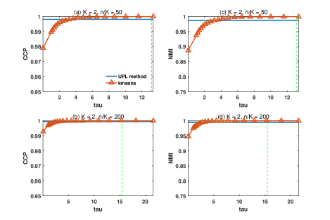
Figure 1: Classification results for K-means for DGP 1 ($K=2$) based on $L_{\tau}=D_{\tau}^{-1/2}A_{\tau}D_{\tau}^{-1/2}$ and for UPL method. The $x$-axis marks $\tau$ values, and the $y$-axis is either CCP (left column) or NMI (right column). The green vertical line in each subplot indicates the estimated $\tau$ value by using the method of Joseph and Yu (2016). The first and second rows correspond to $n/K=50$ and 200, respectively.

In Figures 1 and 2, the first and second rows correspond to the results with $n=100$ and $n=400$, respectively. For each replication, we can compute the feasible $\tau^{\mathrm{JY}}$ as mentioned above. Their averages across all replications are reported in each subplot of Figures 1 and 2. In particular, the green dashed line represents $\tau^{\mathrm{JY}}$, which can be easily compared with the expected average degree, the rightmost vertical border.

We summarize our findings from Figures 1 and 2. First, despite the fact that the minimal degrees for neither DGP satisfies Assumption 3 so that the standard spectral clustering may not be consistent, the regularized spectral clustering performs quite well in both DGPs. This confirms our theoretical finding that the regularization can help to relax the requirement on the minimal degree and to achieve the strong consistency. In addition, when a proper $\tau$ is used, the spectral clustering based on $L_{\tau}$ outperforms the UPL method of Amini et al. (2013). Both results are in line with the theoretical analysis by Joseph and Yu (2016).

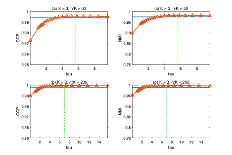
Figure 2: Classification results for DGP 2 ($K=3$) based on $L_{\tau}=D_{\tau}^{-1/2}A_{\tau}D_{\tau}^{-1/2}$. (See the explanations in Figure 1.)

4.2 The DC-SBM

The next two DGPs consider the degree-corrected SBM.

DGP 3: This DGP is the same as DGP 1 except that here $P=\Theta ZBZ^{T}\Theta^{T}$, where $\Theta$ is a diagonal matrix with each diagonal element taking a value from $\{0.5,1.5\}$ with equal probability.

DGP 4: This one is the same as DGP 2 except that here $P=\Theta ZBZ^{T}\Theta^{T}$ and $\Theta$ is generated as in DGP 3.

To compute the feasible regularizer for the DC-SBM, we modify the previous procedure to incorporate the degree heterogeneity. In particular, given $\tau$, by spectral clustering $L_{\tau}^{\prime}$, we can obtain a classification $\hat{Z}=(\hat{Z}_{1},\ldots,\hat{Z}_{n})^{T}$, where $\hat{Z}_{i}$ is a $K$ by 1 vector with its $\hat{g}_{i}$th entry being 1 and the rest being 0 and $\hat{g}_{i}$ is an estimator of node $i$’s community membership. Let $\hat{n}_{k}=\#\{i:\hat{g}_{i}=k\}$. Then we can estimate the block probability matrix $B$ and $\Theta$ by $\hat{B}=[\hat{B}_{kl}]_{1\leq k,l\leq K}$ and $\hat{\Theta}=\mathrm{diag}(\hat{\theta}_{1},\ldots,\hat{\theta}_{n}),$ where $\hat{\theta}_{i}$ is defined in (3.3) and $\hat{B}_{kl}=(\sum\nolimits_{(i,j):\hat{g}_{i}=k,\hat{g}_{j}=l}A_{ij})/(\hat{n}_{k}\hat{n}_{l}).$ Let $\hat{P}=\hat{\Theta}\hat{Z}\hat{B}\hat{Z}^{T}\hat{\Theta}^{T}$, $\hat{\mathcal{D}}_{\tau}=\mathrm{diag}(\hat{P}\iota_{n})+\tau I_{n}$, and $\hat{\mathcal{L}}_{\tau}^{\prime}=\hat{\mathcal{D}}_{\tau}^{-1/2}\hat{P}\hat{\mathcal{D}}_{\tau}^{-1/2}$. Let $\hat{\sigma}_{Kn}^{\prime\tau}$ denote the $K$-th largest eigenvalue of $\hat{\mathcal{L}}_{\tau}^{\prime}$ (in absolute value). Let

$$Q^{\prime}(\tau)=\|L_{\tau}^{\prime}-\hat{\mathcal{L}}_{\tau}^{\prime}\|/|\hat{\sigma}_{Kn}^{\prime\tau}|.$$

We search for some $\tau^{\prime\mathrm{JY}}$ that minimizes $Q^{\prime}(\tau)$ over the same aforementioned grid.

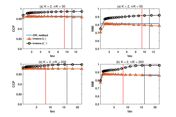
Figure 3: Classification results for DGP 3 ($K=2$, degree-corrected) based on $L_{\tau}^{\prime}=D_{\tau}^{-1/2}AD_{\tau}^{-1/2}$ and $L_{\tau}^{\prime\prime}=D_{\tau}^{-1/2}A_{\tau}D_{\tau}^{-1/2}$. The red and black vertical lines correspond to the optimal regularizers $\tau^{\prime\mathrm{JY}}$ and $\tau^{\prime\prime\mathrm{JY}}$, respectively. (See Figure 1 for the explanation of other features of the figure.)

For DGPs 3 and 4, we report the classification results based on $L_{\tau}^{\prime}=D_{\tau}^{-1/2}AD_{\tau}^{-1/2}$ as the orange lines in Figures 3 and 4. For each subplot, the rightmost border line and the red vertical line represent the averages of $\bar{d}$ and $\tau^{\prime\mathrm{JY}}$, respectively. Figures 3 and 4 show the regularized spectral clustering based on $L_{\tau}^{\prime}$ is slightly outperformed by CPL in DC-SBMs. However, $\tau^{\prime\mathrm{JY}}$ has the close-to-optimal performance in terms of both CCP and NMI over a range of values for $\tau$.

Table 1 reports the classification results for the spectral clustering with $\tau=\tau^{\mathrm{JY}}$ for DGPs 1–2 (or $\tau^{\prime\mathrm{JY}}$ for DGPs 3–4) and $\bar{d}$ in comparison with those for the UPL (or CPL for DGPs 3–4) method over 500 replications. In general, the spectral clustering with $\tau=\tau^{\mathrm{JY}}$ outperforms the UPL method in DGPs 1–2 but slightly underperforms the CPL method for DGPs 3 and 4. In all cases, we observe that the increase of the probability of correct classification as $n$ increases. This is consistent with the theory because both the UPL/CPL method and our regularized spectral clustering method are strongly consistent.

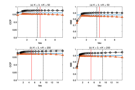
Figure 4: Classification results for DGP 4 ($K=3$, degree-corrected) based on $L_{\tau}^{\prime}=D_{\tau}^{-1/2}AD_{\tau}^{-1/2}$ and $L_{\tau}^{\prime\prime}=D_{\tau}^{-1/2}A_{\tau}D_{\tau}^{-1/2}$. The red and black vertical lines corresponds to the optimal regularizers $\tau^{\prime\mathrm{JY}}$ and $\tau^{\prime\prime\mathrm{JY}}$, respectively. (See Figure 1 for the explanation of other features of the figure.)

Table 1: Comparison of classification results

			CCP			NMI
			Spectral clustering		UPL/CPL	Spectral clustering		UPL/CPL
DGP	$K$	$n/K$	$\bar{d}$	$\tau^{\mathrm{JY}}/\tau^{\prime\mathrm{JY}}$		$\bar{d}$	$\tau^{\mathrm{JY}}/\tau^{\prime\mathrm{JY}}$
1	2	50	0.9998	0.9998	0.9980	0.9989	0.9989	0.9865
	2	200	1.0000	1.0000	0.9994	1.0000	1.0000	0.9947
2	3	50	0.9951	0.9956	0.9941	0.9795	0.9812	0.9748
	3	200	0.9992	0.9995	0.9979	0.9954	0.9972	0.9889
3	2	50	0.9576	0.9596	0.9623	0.7857	0.7964	0.8134
	2	200	0.9764	0.9777	0.9769	0.8564	0.8689	0.8658
4	3	50	0.9460	0.9513	0.9600	0.8308	0.8444	0.8668
	3	200	0.9624	0.9701	0.9745	0.8696	0.8902	0.9022

Figures 3 and 4 also report the classification results based on $L_{\tau}^{\prime\prime}$, which are shown as the dark lines. We find the performance of spectral clustering based on $L_{\tau}^{\prime\prime}$ is better than those using the CPL method. In addition, our choice of $\tau^{\prime\prime\mathrm{JY}}$, marked as the dark vertical line in each subplot, performs well in both DGPs 3 and 4.

5 Proof strategy

In this section we outline the proof strategies for the main results in Section 3.2. First, noting that the regularized spectral clustering for the DC-SBM nests standard SBM without regularization by setting $\tau=0$ and $\theta_{i}=1$ $\forall$ $i=1,\cdots,n$, all the main results in Section 2 follow that in Section 3.2. Second, based on the results in Section 2, the results for the standard SBM with regularization in Section 3.1 can be derived by replacing $B_{0}$, $\mu_{n}$, $\rho_{n}$, and $\sigma_{Kn}$ by their counterparts with regularization, i.e., $B_{0}^{\tau}$, $\mu_{n}^{\tau}$, $\rho_{n}^{\tau}$, and $\sigma_{Kn}^{\tau}$, respectively.

Section 3.2 contains Theorems 3.4, 3.5 and 3.6, Lemma 3.1 and Corollary 3.1. Since the proofs of Theorems 3.4 and 3.6, Lemma 3.1 and Corollary 3.1 are relatively simple, below we focus on the proof strategy for Theorem 3.5.

Theorem 3.5 aims to establish a uniform upper bound for each row of the gap between sample and population eigenvectors (up to some rotation), i.e., $\sup_{i}||\hat{u}_{i}^{T}\hat{O}_{n}-u_{i}^{T}||$, where $\hat{u}_{i}^{T}$ and $u_{i}^{T}$ are the $i$-th rows of $\hat{U}_{1n}$ and $U_{1n}$, respectively. Let $\hat{\Lambda}=L_{\tau}^{\prime}\hat{U}_{1n}\hat{O}_{n}=\hat{U}_{1n}\hat{\Sigma}_{n}\hat{O}_{n}$, $\Lambda=\mathcal{L}_{\tau}^{\prime}U_{1n}=U_{1n}\Sigma_{n}$, $\hat{\Lambda}_{i}=\hat{u}_{i}^{T}\hat{\Sigma}_{n}\hat{O}_{n}$, and $\Lambda_{i}=u_{i}^{T}\Sigma_{n}$. Our proof strategy is to obtain the upper and lower bounds for $(n_{g_{i}^{0}}^{\tau})^{1/2}(\theta_{i}^{\tau})^{-1/2}||\hat{\Lambda}_{i}-\Lambda_{i}||$, both of which involve $(n_{g_{i}^{0}}^{\tau})^{1/2}(\theta_{i}^{\tau})^{-1/2}||\hat{u}_{i}^{T}\hat{O}_{n}-u_{i}^{T}||$. The two bounds produce a contraction mapping for $\sup_{i}(n_{g_{i}^{0}}^{\tau})^{1/2}(\theta_{i}^{\tau})^{-1/2}||\hat{u}_{i}^{T}\hat{O}_{n}-u_{i}^{T}||$. By iterating the contraction mapping sufficiently many times, we obtain the desired bound.

Lower bound. In order to derive the lower bound for $(n_{g_{i}^{0}}^{\tau})^{1/2}||\hat{\Lambda}_{i}-\Lambda_{i}||$, we note that

$$(n_{g_{i}^{0}}^{\tau})^{1/2}(\theta_{i}^{\tau})^{-1/2}\|\hat{\Lambda}_{i}-\Lambda_{i}\| =(n_{g_{i}^{0}}^{\tau})^{1/2}(\theta_{i}^{\tau})^{-1/2}\|\hat{u}_{i}^{T}\hat{\Sigma}_{n}\hat{O}_{n}-u_{i}^{T}\Sigma_{n}\|$$

$$\geq(n_{g_{i}^{0}}^{\tau})^{1/2}(\theta_{i}^{\tau})^{-1/2}\|(\hat{u}_{i}^{T}\hat{O}_{n}-u_{i}^{T})\hat{\Sigma}_{n}\|-(n_{g_{i}^{0}}^{\tau})^{1/2}(\theta_{i}^{\tau})^{-1/2}\|u_{i}^{T}(\hat{\Sigma}_{n}-\Sigma_{n})\|$$

$$\quad\ -(n_{g_{i}^{0}}^{\tau})^{1/2}(\theta_{i}^{\tau})^{-1/2}\|\hat{u}_{i}^{T}(\hat{\Sigma}_{n}\hat{O}_{n}-\hat{O}_{n}\hat{\Sigma}_{n})\|$$

$$\equiv I_{i}-II_{i}-III_{i}.$$ (5.1)

Clearly, by the Hoffman-Wielandt inequality, Lemma 3.1, and Assumption 13.2,

$$|\hat{\sigma}_{Kn}|\geq|\sigma_{Kn}|-7\left(\frac{\log(n)}{\mu_{n}^{\tau}\sigma_{Kn}^{2}}\right)^{1/2}|\sigma_{Kn}|\geq 0.999|\sigma_{Kn}|\quad a.s.,$$

and thus,

$$\sup_{i}I_{i}\geq 0.999|\sigma_{Kn}|\Gamma_{n}\quad a.s.,$$

where $\Gamma_{n}=\sup_{i}|(n_{g_{i}^{0}}^{\tau})^{1/2}(\theta_{i}^{\tau})^{-1/2}\|\hat{u}_{i}^{T}\hat{O}_{n}-u_{i}^{T}\|$. It is the leading term of the lower bound involving $\Gamma_{n}$. In the online Appendix B, we show that $\sup_{i}II_{i}\leq 7(\log(n)/\mu_{n}^{\tau})^{1/2}\quad a.s.$ and $\sup_{i}III_{i}\leq 34(\log(n)/\mu_{n}^{\tau})^{1/2}|\sigma_{Kn}|^{-1}(\Gamma_{n}+1)\quad a.s.$ It follows that

$$\sup_{i}(n_{g_{i}^{0}}^{\tau})^{1/2}(\theta_{i}^{\tau})^{-1/2}\|\hat{\Lambda}_{i}-\Lambda_{i}\|\geq (0.999|\sigma_{Kn}|-34(\log(n)/\mu_{n}^{\tau})^{1/2}|\sigma_{Kn}^{-1}|)\Gamma_{n}-41(\log(n)/\mu_{n}^{\tau})^{1/2}|\sigma_{Kn}^{-1}|$$

$$\geq 0.99|\sigma_{Kn}|\Gamma_{n}-41(\log(n)/\mu_{n}^{\tau})^{1/2}|\sigma_{Kn}^{-1}|,$$ (5.2)

where we use the fact that $34(\log(n)/\mu_{n}^{\tau})^{1/2}|\sigma_{Kn}^{-2}|\leq 0.09.$

Upper bound. To derive the upper bound for $\sup_{i}(n_{g_{i}^{0}}^{\tau})^{1/2}(\theta_{i}^{\tau})^{-1/2}\|\hat{\Lambda}_{i}-\Lambda_{i}\|$, we first denote $\tilde{\Lambda}=D_{\tau}^{-1/2}PD_{\tau}^{-1/2}U_{1n}$ and $\tilde{\Lambda}_{i}=(\hat{d}_{i}^{\tau})^{-1/2}[P]_{i\cdot}D_{\tau}^{-1/2}U_{1n}$ as the $i$-th row of $\tilde{\Lambda}$. Then, we have

$$\sup_{i}(n_{g_{i}^{0}}^{\tau})^{1/2}(\theta_{i}^{\tau})^{-1/2}\|\hat{\Lambda}_{i}-\Lambda_{i}\| \leq\sup_{i}(n_{g_{i}^{0}}^{\tau})^{1/2}(\theta_{i}^{\tau})^{-1/2}\|\Lambda_{i}-\tilde{\Lambda}_{i}\|+\sup_{i}(n_{g_{i}^{0}}^{\tau})^{1/2}(\theta_{i}^{\tau})^{-1/2}\|\hat{\Lambda}_{i}-\tilde{\Lambda}_{i}\|$$

$$\equiv T_{1}+T_{2}.$$ (5.3)

For $T_{2},$ we have

$$T_{2} =\sup_{i}(n_{g_{i}^{0}}^{\tau})^{1/2}(\theta_{i}^{\tau})^{-1/2}\|(\hat{d}_{i}^{\tau})^{-1/2}[A]_{i\cdot}D_{\tau}^{-1/2}\hat{U}_{1n}\hat{O}_{n}-(\hat{d}_{i}^{\tau})^{-1/2}[P]_{i\cdot}D_{\tau}^{-1/2}U_{1n}\|$$

$$\leq\sup_{i}(n_{g_{i}^{0}}^{\tau})^{1/2}(\theta_{i}^{\tau})^{-1/2}(\hat{d}_{i}^{\tau})^{-1/2}\|[P]_{i\cdot}D_{\tau}^{-1/2}(\hat{U}_{1n}\hat{O}_{n}-U_{1n})\|$$

$$+\sup_{i}(n_{g_{i}^{0}}^{\tau})^{1/2}(\theta_{i}^{\tau})^{-1/2}(\hat{d}_{i}^{\tau})^{-1/2}\|([A]_{i\cdot}-[P]_{i\cdot})(D_{\tau}^{-1/2}-\mathcal{D}_{\tau}^{-1/2})\hat{U}_{1n}\hat{O}_{n}\|$$

$$+\sup_{i}(n_{g_{i}^{0}}^{\tau})^{1/2}(\theta_{i}^{\tau})^{-1/2}(\hat{d}_{i}^{\tau})^{-1/2}\|([A]_{i\cdot}-[P]_{i\cdot})\mathcal{D}_{\tau}^{-1/2}\hat{U}_{1n}\hat{O}_{n}\|$$

$$\equiv T_{2,1}+T_{2,2}+T_{2,3}.$$ (5.4)

Lemma C.5 in the online Appendix C provides the upper bounds for $T_{1}$, $T_{2,1}$, $T_{2,2}$, and $T_{2,3}$. Taking $T_{2,3}$ as an example, we note that

$$T_{2,3}=\sup_{i}\sup_{h=\hat{U}_{1n}\hat{O}_{n}f,f\in S^{K-1}}(n_{g_{i}^{0}}^{\tau})^{1/2}(\theta_{i}^{\tau})^{-1/2}\sum_{j=1}^{n}(A_{ij}-P_{ij})(\hat{d}_{i}^{\tau}d_{j}^{\tau})^{-1/2}h_{j}.$$

Here, $h_{j}$ denotes the $j$th element of $h.$ Lemma C.4 builds a Bernstein-type concentration inequality to upper bound $T_{2,3}$, which involves the $l_{\infty}$ and $l_{2}$ norms of $h$, In particular, $||h||_{\infty}$ depends on the rough upper bound $\delta_{n}^{(0)}$ for $\Gamma_{n}$. One of the technical difficulties is that, due to the correlation between the sample graph Laplacian and its eigenvectors, the sequence of random variables $A_{ij}:j=1,\cdots,n$ are not independent of $h=\hat{U}_{1n}\hat{O}_{n}f$ for some $f\in S^{K-1}$. To deal with it, we rely on the “leave-one-out” technique used in Abbe et al. (2017), Bean et al. (2013), Javanmard and Montanari (2015), and Zhong and Boumal (2018). The idea is to approximate the eigenvector by a vector which is independent of one particular row of the sample graph Laplacian. This helps to restore the independence. Then, the approximation errors are bounded in Lemma C.7, which further calls upon Lemmas C.6 and C.8.

At the end, Lemma C.5 establishes that

$$\sup_{i}(n_{g_{i}^{0}}^{\tau})^{1/2}(\theta_{i}^{\tau})^{-1/2}\|\hat{\Lambda}_{i}-\Lambda_{i}\|$$

$$\leq 3450C_{1}c_{1}^{-1/2}\rho_{n}\log^{1/2}(n)(\mu_{n}^{\tau})^{-1/2}|\sigma_{Kn}^{-1}|\biggl{[}\delta_{n}^{(0)}+1+\rho_{n}+\frac{\left(\frac{1}{K}+\frac{\log(5)}{\log(n)}\right)^{1/2}\rho_{n}^{1/2}\overline{\theta}^{1/4}}{\underline{\theta}^{1/4}}\biggr{]},\quad a.s.,$$ (5.5)

where we can choose $\delta_{n}^{(0)}=n^{1/2}\underline{\theta}^{-1/2}$. Combining the lower and upper bounds in (5.2) and (5.5) for $\sup_{i}(n_{g_{i}^{0}}^{\tau})^{1/2}(\theta_{i}^{\tau})^{-1/2}\|\hat{\Lambda}_{i}-\Lambda_{i}\|$ and applying Assumption 13, we have

$$0.001\delta_{n}^{(0)}+3527C_{1}c_{1}^{-1/2}\eta_{n}\geq\Gamma_{n},$$ (5.6)

where $\eta_{n}$ is defined in Theorem 3.5.

Iteration. (5.6) suggests that the initial rough upper bound $\delta_{n}^{(0)}$ for $\Gamma_{n}$ can be refined to $\delta_{n}^{(1)}\equiv 0.001\delta_{n}^{(0)}+3527C_{1}c_{1}^{-1/2}\eta_{n}$. Then we can take this new upper bound into the previous calculations to obtain

$$0.001\delta_{n}^{(1)}+3527C_{1}c_{1}^{-1/2}\eta_{n}\geq\Gamma_{n}.$$

Therefore, we have constructed a contraction mapping, through which we can refine our upper bound for $\Gamma_{n}$ via iterations. We iterate the above calculation $t$ times for some arbitrary integer $t$, and obtain that

$$\Gamma_{n}\leq\delta_{n}^{(t)},\quad\delta_{n}^{(t)}=0.001\delta_{n}^{(t-1)}+3527C_{1}c_{1}^{-1/2}\eta_{n}.$$

This implies

$$\delta_{n}^{(t)}=\left(0.001\right)^{t}\biggl{[}\delta_{n}^{(0)}-3527C_{1}c_{1}^{-1/2}\eta_{n}\biggr{]}+3527C_{1}c_{1}^{-1/2}\eta_{n}.$$

Letting $t=n$, we have

$$\Gamma_{n}\leq\delta_{n}^{(n)}\leq 1000^{-n}n^{1/2}\underline{\theta}^{-1/2}+3527C_{1}c_{1}^{-1/2}\eta_{n}\leq 3528C_{1}c_{1}^{-1/2}\eta_{n},$$

where we denote $C^{\ast}$ in Theorem 3.5 as $3528C_{1}c_{1}^{-1/2}$ and we use the fact that it is possible to choose $\delta_{n}^{(0)}=n^{1/2}\underline{\theta}^{-1/2}$ as the initial rough bound for $\Gamma_{n}$.

6 Conclusion

In this paper, we show that under suitable conditions, the K-means algorithm applied to the eigenvectors of the graph Laplacian associated with its first few largest eigenvalues can classify all individuals into the true community uniformly correctly almost surely in large samples. In the special case where the number of communities is fixed and the probability block matrix has minimal eigenvalue bounded away from zero, the strong consistency essentially requires that the minimal degree diverges to infinity at least as fast as $\log(n)$, which is the minimal rate requirement for the strong consistency discussed in Abbe (2018). Similar results are also established for the regularized DC-SBMs. The simulations confirm our theoretical findings and indicate that an adaptive procedure can improve the finite sample performance of the regularized spectral clustering for DC-SBMs.

Online Supplement to “Strong Consistency of Spectral Clustering for Stochastic Block Models”

Appendix A Proofs of the results in Section 2

In this section, we prove the main results in Section 2, viz., Theorems 2.1–2.3, Lemmas 2.1–2.2, and Corollary 2.1. In particular, we note that the standard SBM is a special case of regularized DC-SBM with regularizer $\tau=0$ and degree-corrected parameter $\theta_{i}=1$. Therefore, Lemma 2.1 and Theorem 2.2 follow Lemma 3.1 and Theorem 3.5, respectively.

Proof of Theorem 2.1.

By the proof of Rohe et al. (2011, Lemma 3.1), we have $\mathcal{L}=n^{-1}ZB_{0}Z^{T}$. Therefore, $\mathcal{L}^{2}=n^{-1}ZB_{0}(Z^{T}Z/n)B_{0}Z^{T}.$ Let $\Pi_{n}=Z^{T}Z/n=\text{diag}(\pi_{1n},\ldots,\pi_{Kn})$. By the spectral decomposition in Assumption 1, we have

$$\Pi_{n}^{1/2}B_{0}\Pi_{n}B_{0}\Pi_{n}^{1/2}=S_{n}\Omega_{n}^{2}S_{n}^{T},$$ (A.1)

where $\Omega_{n}=\text{diag}(\omega_{1n},\ldots,\omega_{Kn})$ such that $|\omega_{1n}|\geq|\omega_{2n}|\geq\cdots\geq|\omega_{Kn}|>0$ and $S_{n}$ is a $K\times K$ matrix such that $S_{n}^{T}S_{n}=I_{K}.$ Let $U_{1n}^{\ast}=Z(Z^{T}Z)^{-1/2}S_{n}$. Then, we have

$$U_{1n}^{\ast}\Omega_{n}^{2}U_{1n}^{\ast T}=\mathcal{L}^{2}=U_{1n}\Sigma_{1n}^{2}U_{1n}^{T}.$$ (A.2)

In addition, $U_{1n}^{\ast T}U_{1n}^{\ast}=S_{n}^{T}S_{n}=I_{K}$. Therefore the columns of $U_{1n}^{\ast}$ are the eigenvectors of $\mathcal{L}$ associated with eigenvalues $\sigma_{1n},\ldots,\sigma_{Kn}$, up to sign normalization. Without loss of generality (W.l.o.g.), we can take $U_{1n}=U_{1n}^{\ast}$ and $\Omega_{n}=\Sigma_{1n}$.

Furthermore, if node $i$ is in cluster $C_{k_{1}}$, then $z_{i}^{T}(Z^{T}Z)^{-1/2}S_{n}=n_{k_{1}}^{-1/2}[S_{n}]_{k_{1}\cdot}$, where $[S_{n}]_{k\cdot}$ denotes the $k$-th row of $S_{n}$. Therefore, by Assumption 2 and the fact that $\|[S_{n}]_{k_{1}\cdot}\|=1$,

$$(n/K)^{1/2}\|z_{i}^{T}(Z^{T}Z)^{-1/2}S_{n}\|\leq c_{1}^{-1/2}\|[S_{n}]_{k_{1}\cdot}\|=c_{1}^{-1/2}.$$

Taking $\sup_{i}$ on both sides establishes the first desired result.

Similarly, by Assumption 2, we can also establish the lower bound: for node $j$ in cluster $C_{k_{2}}$ with $k_{1}\neq k_{2}$

$$(n/K)^{1/2}\|(z_{i}-z_{j})^{T}(Z^{T}Z)^{-1/2}S_{n}\|=||n_{k_{1}}^{-1/2}[S_{n}]_{k_{1}\cdot}-n_{k_{2}}^{-1/2}[S_{n}]_{k_{2}\cdot}||\geq C_{1}^{-1/2}\sqrt{2}=\underline{c}>0.$$

This concludes the proof.

   

Proof of Lemma 2.1.

Lemma 2.1 is a special case of Lemma 3.1 with $\theta_{i}=1$ for $i=1,\cdots,n$ and $\tau=0$. We prove the general result in Lemma 3.1 later.

   

Proof of Theorem 2.2.

Theorem 2.2 is a special case of Theorem 3.5 when $\theta_{i}=1$ for $i=1,\cdots,n$ and $\tau=0$. We prove Theorem 3.5 with $C^{\ast}=3528C_{1}c_{1}^{-1/2}$ later.

   

Proof of Lemma 2.2.

Let $Q_{n}(\mathcal{A})=\sum_{k=1}^{K}\min_{1\leq l\leq K}\|\beta_{kn}-\alpha_{l}\|^{2}\pi_{kn}.$ We first derive the convergence rate of $\widehat{Q}_{n}(\mathcal{A})-Q_{n}(\mathcal{A})$ uniformly over $\mathcal{A}\in\mathcal{M}=\{(\alpha_{1},\ldots,\alpha_{K}):\sup_{1\leq k\leq K}\|\alpha_{k}\|\leq 2M\}$ for some constant $M$ independent of $n$. Let $R_{n}=\sup_{i}\|\hat{\beta}_{in}-\beta_{g_{i}^{0}n}\|$ . Then, by Assumption 4.3,

$$R_{n}\leq c_{2n}\leq M\quad a.s.$$ (A.3)

In addition,

$$\|\hat{\beta}_{in}-\alpha_{l}\|^{2} \geq\|\beta_{g_{i}^{0}n}-\alpha_{l}\|^{2}-2|(\beta_{g_{i}^{0}n}-\hat{\beta}_{in})^{T}(\beta_{g_{i}^{0}n}-\alpha_{l})|-\|\beta_{g_{i}^{0}n}-\hat{\beta}_{in}\|^{2}$$

$$\geq\|\beta_{g_{i}^{0}n}-\alpha_{l}\|^{2}-2\|\beta_{g_{i}^{0}n}-\hat{\beta}_{in}\|_{1}\|\beta_{g_{i}^{0}n}-\alpha_{l}\|_{\infty}-R_{n}^{2}$$

$$\geq\|\beta_{g_{i}^{0}n}-\alpha_{l}\|^{2}-2\sqrt{K}R_{n}\|\beta_{g_{i}^{0}n}-\alpha_{l}\|-R_{n}^{2}$$

$$\geq\|\beta_{g_{i}^{0}n}-\alpha_{l}\|^{2}-2\sqrt{K}R_{n}(\|\beta_{g_{i}^{0}n}\|+\|\alpha_{l}\|)-R_{n}^{2},$$

where the third inequality follows the Cauchy–Schwarz inequality with the fact that both $\beta_{g_{i}^{0}n}$ and $\hat{\beta}_{in}$ are $K\times 1$ vectors. Taking $\min_{1\leq l\leq K}$ on both sides and averaging over $i$, we have

$$\widehat{Q}_{n}(\mathcal{A})\geq Q_{n}(\mathcal{A})-(6\sqrt{K}+1)Mc_{2n}.$$

Similarly, we have $\widehat{Q}_{n}(\mathcal{A})\leq Q_{n}(\mathcal{A})+(6\sqrt{K}+1)Mc_{2n}.$ By (A.3),

$$\breve{R}_{n}\equiv\sup_{\mathcal{A}\in\mathcal{M}}|\widehat{Q}_{n}(\mathcal{A})-Q_{n}(\mathcal{A})|\leq(6\sqrt{K}+1)Mc_{2n}\quad a.s.$$

Next, we show $\widehat{\mathcal{A}}_{n}\in\mathcal{M}$. Denote $\widehat{\mathcal{A}}_{n}=\{\widehat{\alpha}_{1},\ldots,\widehat{\alpha}_{K}\}$. By Assumption 4.1,

$$\sup_{i}\|\hat{\beta}_{in}\|\leq R_{n}+\sup_{1\leq k\leq K}\|\beta_{kn}\|\leq 2M.$$

Denote $I_{n}(k)=\{i:k=\operatorname*{arg\,min}_{1\leq l\leq K}\|\hat{\beta}_{in}-\widehat{\alpha}_{l}\|\}$ for some $k\leq K$. If $\|\widehat{\alpha}_{k}\|>2M$ and $I_{n}(k)=\emptyset$, then we can choose

$$\widehat{\mathcal{A}}_{n}^{\prime}=\{\widehat{\alpha}_{1},\ldots,\widehat{\alpha}_{k-1},\widehat{\alpha}_{k}^{\prime},\widehat{\alpha}_{k+1},\ldots,\widehat{\alpha}_{K}\},$$

where $\widehat{\alpha}_{k}^{\prime}=\hat{\beta}_{in}$ for some arbitrary $i\leq n$. Therefore, we have $\|\widehat{\alpha}_{k}^{\prime}\|\leq 2M<\|\widehat{\alpha}_{k}\|$ and $\widehat{Q}_{n}(\widehat{\mathcal{A}}_{n}^{\prime})<\widehat{Q}_{n}(\widehat{\mathcal{A}}_{n}),$ which is a contradiction. On the other hand, if $\|\widehat{\alpha}_{k}\|>2M$ and $I_{n}(k)\neq\emptyset$, then we can choose

$$\widehat{\mathcal{A}}_{n}^{\prime}=\{\widehat{\alpha}_{1},\ldots,\widehat{\alpha}_{k-1},\widehat{\alpha}_{k}^{\prime},\widehat{\alpha}_{k+1},\ldots,\widehat{\alpha}_{K}\},$$

where $\widehat{\alpha}_{k}^{\prime}=\frac{1}{|I_{n}(k)|}\sum_{i\in I_{n}}\hat{\beta}_{in}$ and $|I_{n}(k)|$ is the cardinality of $I_{n}(k)$. This means $\|\widehat{\alpha}_{k}^{\prime}\|\leq 2M<\|\widehat{\alpha}_{k}\|$ and $\widehat{Q}_{n}(\widehat{\mathcal{A}}_{n}^{\prime})<\widehat{Q}_{n}(\widehat{\mathcal{A}}_{n})$, which is a contradiction too. Therefore, $\|\widehat{\alpha}_{k}\|\leq 2M$. Since $k$ is arbitrary, $\widehat{\mathcal{A}}_{n}\in\mathcal{M}$.

Third, we show for any $\eta>0$,

$$\inf_{\mathcal{A}:H(\mathcal{A},\mathcal{B}_{n})>\eta}Q_{n}(\mathcal{A})\geq\frac{c_{1}}{K}\min(\eta^{2},c_{1n}^{2}/2),$$ (A.4)

where $\mathcal{B}_{n}=\{\beta_{1n},\ldots,\beta_{Kn}\}$ and $c_{1}$ is the constant defined in Assumption 4.2. If there exist some $l_{0}\in\{1,\ldots,K\}$ and two indexes $k_{1}$ and $k_{2}$ such that

$$l_{0}=\operatorname*{arg\,min}_{1\leq l\leq K}\|\beta_{k_{1}n}-\alpha_{l}\|=\operatorname*{arg\,min}_{1\leq l\leq K}\|\beta_{k_{2}n}-\alpha_{l}\|,$$

then by Assumption 4.2

$$Q_{n}(\mathcal{A}) \geq\pi_{k_{1}n}\|\beta_{k_{1}n}-\alpha_{l_{0}}\|^{2}+\pi_{k_{2}n}\|\beta_{k_{2}n}-\alpha_{l_{0}}\|^{2}$$

$$\geq\frac{c_{1}}{2K}(\|\beta_{k_{1}n}-\alpha_{l_{0}}\|+\|\beta_{k_{2}n}-\alpha_{l_{0}}\|)^{2}\geq\frac{c_{1}}{2K}\|\beta_{k_{1}n}-\beta_{k_{2},n}\|^{2}\geq\frac{c_{1}c_{1n}^{2}}{2K}.$$

On the other hand, if there does not exist such an $l_{0}$, then there is a one-to-one mapping $h:\{1,\ldots,K\}\mapsto\{1,\ldots,K\}$ such that

$$h(k)=\operatorname*{arg\,min}_{1\leq l\leq K}\|\beta_{kn}-\alpha_{l}\|.$$

Therefore,

$$Q_{n}(\mathcal{A})=\sum_{k=1}^{K}\pi_{kn}\|\beta_{kn}-\alpha_{h(k)}\|^{2}\geq(\inf_{k}\pi_{kn})H^{2}(\mathcal{A},\mathcal{B}_{n})\geq c_{1}\eta^{2}/K.$$

Last, we show $H(\widehat{\mathcal{A}}_{n},\mathcal{B}_{n})\leq(15M/c_{1})^{1/2}c_{2n}^{1/2}K^{3/4}$. For any $\varepsilon>0$ and sufficiently large $C_{2}$,

$$P(H(\widehat{\mathcal{A}}_{n},\mathcal{B}_{n})\geq(15M/c_{1})^{1/2}c_{2n}^{1/2}K^{3/4}\quad i.o.)$$

$$=P(H(\widehat{\mathcal{A}}_{n},\mathcal{B}_{n})\geq(15M/c_{1})^{1/2}c_{2n}^{1/2}K^{3/4},Q_{n}(\widehat{\mathcal{A}}_{n})\geq Q_{n}(\mathcal{B}_{n})$$

$$+\min(15Mc_{2n}K^{1/2},c_{1}c_{1n}^{2}/(2K))\quad i.o.)$$

$$\leq P(\widehat{Q}_{n}(\widehat{\mathcal{A}}_{n})+\breve{R}_{n}\geq\widehat{Q}_{n}(\mathcal{B}_{n})-\breve{R}_{n}+\min(15Mc_{2n}K^{1/2},c_{1}c_{1n}^{2}/(2K))\quad i.o.)$$

$$=P(2\breve{R}_{n}\geq\widehat{Q}_{n}(\mathcal{B}_{n})-\widehat{Q}_{n}(\widehat{\mathcal{A}}_{n})+\min(15Mc_{2n}K^{1/2},c_{1}c_{1n}^{2}/(2K))\quad i.o.)$$

$$\leq P(2\breve{R}_{n}\geq\min(15Mc_{2n}K^{1/2},c_{1}c_{1n}^{2}/(2K))\quad i.o.)=0,$$

where the first equality holds due to (A.4) and the fact that $Q_{n}(\mathcal{B}_{n})=0$, the last inequality holds because $\widehat{Q}_{n}(\mathcal{B}_{n})-\widehat{Q}_{n}(\widehat{\mathcal{A}}_{n})\geq 0$, and the last equality holds because, by Assumption 4.3,

$$2\breve{R}_{n}\leq 2(6\sqrt{K}+1)Mc_{2n}<15\sqrt{K}Mc_{2n}\leq c_{1}c_{1n}^{2}/(2K).$$

This concludes the proof.

   

Proof of Theorem 2.3.

By Lemma 2.2 and Assumption 4.2 and (iii), for each $n$, there is a one-to-one mapping $F_{n}:\{1,\ldots,K\}\mapsto\{1,\ldots,K\}$, such that

$$\sup_{k}\|\widehat{\alpha}_{kn}-\beta_{F_{n}(k)n}\|\leq(15M/c_{1})^{1/2}c_{2n}^{1/2}K^{3/4}\quad a.s.$$

W.l.o.g., we can assume $F_{n}(k)=k$ such that

$$\tilde{R}_{n}\equiv\sup_{k}\|\widehat{\alpha}_{kn}-\beta_{kn}\|\leq(15M/c_{1})^{1/2}c_{2n}^{1/2}K^{3/4}\quad a.s.$$ (A.5)

If $\hat{g}_{i}\neq g_{i}^{0}$, then $\|\hat{\beta}_{in}-\widehat{\alpha}_{\hat{g}_{i}n}\|\leq\|\hat{\beta}_{in}-\widehat{\alpha}_{g_{i}^{0}n}\|.$ This, in conjunction with the triangle inequality, implies that

$$\|\widehat{\alpha}_{\hat{g}_{i}n}-\widehat{\alpha}_{g_{i}^{0}n}\|-\|\hat{\beta}_{in}-\widehat{\alpha}_{g_{i}^{0}n}\|\leq\|\hat{\beta}_{in}-\widehat{\alpha}_{\hat{g}_{i}n}\|\leq\|\hat{\beta}_{in}-\widehat{\alpha}_{g_{i}^{0}n}\|.$$

It follows that $\|\hat{\beta}_{in}-\widehat{\alpha}_{g_{i}^{0}n}\|\geq\frac{1}{2}\|\widehat{\alpha}_{\hat{g}_{i}n}-\widehat{\alpha}_{g_{i}^{0}n}\|.$ By (A.3), (A.5), and the repeated use of the triangle inequality, we have

$$c_{2n}+\tilde{R}_{n} \geq\|\hat{\beta}_{in}-\beta_{g_{i}^{0}n}\|+\|\beta_{g_{i}^{0}n}-\widehat{\alpha}_{g_{i}^{0}n}\|\text{ }$$

$$\geq\|\hat{\beta}_{in}-\widehat{\alpha}_{g_{i}^{0}n}\|\geq\frac{1}{2}\|\widehat{\alpha}_{\hat{g}_{i}n}-\widehat{\alpha}_{g_{i}^{0}n}\|\text{ }$$

$$=\frac{1}{2}\|(\beta_{\hat{g}_{i}n}-\beta_{g_{i}^{0}n})+(\widehat{\alpha}_{\hat{g}_{i}n}-\beta_{\hat{g}_{i}n})+(\beta_{g_{i}^{0}n}-\widehat{\alpha}_{g_{i}^{0}n})\|$$

$$\geq\frac{1}{2}\|\beta_{\hat{g}_{i}n}-\beta_{g_{i}^{0}n}\|-\tilde{R}_{n}\geq c_{1n}/2-\tilde{R}_{n}.$$

This implies $1\{\hat{g}_{i}\neq g_{i}^{0}\}\leq 1\{R_{n}+2\tilde{R}_{n}\geq c_{1n}/2\}.$ Noting that the RHS of the above display is independent of $i$, we have

$$P(\sup_{i}1\{\hat{g}_{i}\neq g_{i}^{0}\}>0\quad i.o.) \leq P(c_{2n}+2\tilde{R}_{n}\geq c_{1n}/2\quad i.o.)$$

$$=P(c_{2n}+2(15M/c_{1})^{1/2}c_{2n}^{1/2}K^{3/4}\geq c_{1n}/2\quad i.o.)$$

$$=0\text{ under Assumption \ref{ass:theta}.3.}$$

This concludes the proof.

   

Proof of Corollary 2.1.

We note that $\beta_{kn}=(K\pi_{kn})^{-1/2}[S_{n}\hat{O}_{n}^{T}]_{k\cdot}$, $M=||\beta_{kn}||\leq c_{1}^{-1/2}$, $\hat{\beta}_{in}=(n/K)^{1/2}\hat{u}_{1i}^{T}$, $c_{1n}=C_{1}^{-1/2}\sqrt{2}>0$, and

$$c_{2n}=C^{\ast}\frac{\rho_{n}\log^{1/2}(n)}{\mu_{n}^{1/2}\sigma_{Kn}^{2}}\left(1+\rho_{n}+\left(\frac{1}{K}+\frac{\log(5)}{\log(n)}\right)^{1/2}\rho_{n}^{1/2}\right).$$

Then, by Theorem 2.3 and Assumption 3, we have

$$(2c_{2n}c_{1}^{1/2}+16K^{3/4}M^{1/2}c_{2n}^{1/2})^{2}\leq 16.02^{2}K^{3/2}Mc_{2n}\leq 257K^{3/2}c_{1}^{-1/2}c_{2n}\leq 2c_{1}C_{1}^{-1},$$

where the first inequality holds because by Assumption 3 and the facts that $C^{\ast}=3528C_{1}c_{1}^{-1/2}$ and

$$2c_{2n}c_{1}^{1/2}\leq 2(10^{-8}C_{1}^{-1}c_{1}^{1/2}C^{\ast})^{1/2}c_{2n}^{1/2}\leq 0.02c_{2n}^{1/2}.$$

This verifies Assumption 4.3.

   

Proof of Lemma 2.3.

Following the first step in the proof of Lemma 2.2, we can show that

$$\breve{R}_{n}\equiv\sup_{\mathcal{A}}|\widetilde{Q}_{n}(\mathcal{A})-Q_{n}(\mathcal{A})|\leq c_{2n}.$$ (A.6)

Suppose $H(\mathcal{A},\mathcal{B}_{n})\geq\eta$ for any $\eta>0$. Then, by Step 3 in the proof of Lemma 2.2, if there exist some $l_{0}\in\{1,\ldots,K\}$ and two indexes $k_{1}$ and $k_{2}$ such that

$$l_{0}=\operatorname*{arg\,min}_{1\leq l\leq K}\|\beta_{k_{1}n}-\alpha_{l}\|=\operatorname*{arg\,min}_{1\leq l\leq K}\|\beta_{k_{2}n}-\alpha_{l}\|,$$

then by Assumption 4.2

$$Q_{n}(\mathcal{A}) \geq\pi_{k_{1}n}\|\beta_{k_{1}n}-\alpha_{l_{0}}\|+\pi_{k_{2}n}\|\beta_{k_{2}n}-\alpha_{l_{0}}\|$$

$$\geq\frac{c_{1}}{K}\|\beta_{k_{1}n}-\beta_{k_{2},n}\|\geq c_{1}c_{1n}/K.$$

On the other hand, if there does not exist such an $l_{0}$, then there is a one-to-one mapping $h:\{1,\ldots,K\}\mapsto\{1,\ldots,K\}$ such that

$$h(k)=\operatorname*{arg\,min}_{1\leq l\leq K}\|\beta_{kn}-\alpha_{l}\|.$$

Therefore,

$$Q_{n}(\mathcal{A})=\sum_{k=1}^{K}\pi_{kn}\|\beta_{kn}-\alpha_{h(k)}\|\geq(\inf_{k}\pi_{kn})H(\mathcal{A},\mathcal{B}_{n})\geq c_{1}\eta/K$$

and

$$\inf_{\mathcal{A}:H(\mathcal{A},\mathcal{B}_{n})>\eta}Q_{n}(\mathcal{A})\geq\frac{c_{1}(c_{1n}\wedge\eta)}{K}.$$ (A.7)

By Step 4 of the proof of Lemma 2.2 and letting $\eta=\frac{3Kc_{2n}}{c_{1}}$, we have

$$P(H(\widetilde{\mathcal{A}}_{n},\mathcal{B}_{n})\geq\frac{3Kc_{2n}}{c_{1}}\quad i.o.)$$

$$= P(H(\widetilde{\mathcal{A}}_{n},\mathcal{B}_{n})\geq\frac{3Kc_{2n}}{c_{1}},Q_{n}(\widetilde{\mathcal{A}}_{n})\geq Q_{n}(\mathcal{B}_{n})+\min\frac{c_{1}(c_{1n}\wedge\frac{3Kc_{2n}}{c_{1}})}{K}\quad i.o.)$$

$$\leq P(\widetilde{Q}_{n}(\widetilde{\mathcal{A}}_{n})+\breve{R}_{n}\geq\widetilde{Q}_{n}(\mathcal{B}_{n})-\breve{R}_{n}+3c_{2n}\quad i.o.)$$

$$\leq P(2\breve{R}_{n}\geq 3c_{2n}\quad i.o.)$$

$$\leq P(2c_{2n}\geq 3c_{2n}\quad i.o.)=0,$$

where the first equality is due to (A.7), the first inequality is due to Assumption 6.2, the second inequality is because $\widetilde{Q}_{n}(\widetilde{\mathcal{A}}_{n})\leq\widetilde{Q}_{n}(\mathcal{\beta}_{n})$, and the third inequality is due to (A.6).

   

Proof of Theorem 2.4.

By Lemma 2.3 and Assumption 4.2, for each $n$, there is a one-to-one mapping $F_{n}:\{1,\ldots,K\}\mapsto\{1,\ldots,K\}$, such that

$$\sup_{k}\|\widetilde{\alpha}_{kn}-\beta_{F_{n}(k)n}\|\leq 3Kc_{1}^{-1}c_{2n}\quad a.s.$$

W.l.o.g., we can assume $F_{n}(k)=k$ such that

$$\tilde{R}_{n}\equiv\sup_{k}\|\widetilde{\alpha}_{kn}-\beta_{kn}\|\leq 3Kc_{1}^{-1}c_{2n}\quad a.s.$$ (A.8)

If $\tilde{g}_{i}\neq g_{i}^{0}$, then $\|\hat{\beta}_{in}-\widetilde{\alpha}_{\tilde{g}_{i}n}\|\leq\|\hat{\beta}_{in}-\widetilde{\alpha}_{g_{i}^{0}n}\|.$ This, in conjunction with the triangle inequality, implies that

$$\|\widetilde{\alpha}_{\tilde{g}_{i}n}-\widetilde{\alpha}_{g_{i}^{0}n}\|-\|\hat{\beta}_{in}-\widetilde{\alpha}_{g_{i}^{0}n}\|\leq\|\hat{\beta}_{in}-\widetilde{\alpha}_{\tilde{g}_{i}n}\|\leq\|\hat{\beta}_{in}-\widetilde{\alpha}_{g_{i}^{0}n}\|.$$

It follows that $\|\hat{\beta}_{in}-\widetilde{\alpha}_{g_{i}^{0}n}\|\geq\frac{1}{2}\|\widetilde{\alpha}_{\tilde{g}_{i}n}-\widetilde{\alpha}_{g_{i}^{0}n}\|.$ By (A.6), (A.8), and the repeated use of the triangle inequality, we have

$$c_{2n}+\tilde{R}_{n} \geq\|\hat{\beta}_{in}-\beta_{g_{i}^{0}n}\|+\|\beta_{g_{i}^{0}n}-\widetilde{\alpha}_{g_{i}^{0}n}\|\text{ }$$

$$\geq\|\hat{\beta}_{in}-\widetilde{\alpha}_{g_{i}^{0}n}\|\geq\frac{1}{2}\|\widetilde{\alpha}_{\tilde{g}_{i}n}-\widetilde{\alpha}_{g_{i}^{0}n}\|\text{ }$$

$$=\frac{1}{2}\|(\beta_{\tilde{g}_{i}n}-\beta_{g_{i}^{0}n})+(\widetilde{\alpha}_{\tilde{g}_{i}n}-\beta_{\tilde{g}_{i}n})+(\beta_{g_{i}^{0}n}-\widetilde{\alpha}_{g_{i}^{0}n})\|$$

$$\geq\frac{1}{2}\|\beta_{\tilde{g}_{i}n}-\beta_{g_{i}^{0}n}\|-\tilde{R}_{n}\geq c_{1n}/2-\tilde{R}_{n}.$$

This implies $1\{\tilde{g}_{i}\neq g_{i}^{0}\}\leq 1\{c_{2n}+2\tilde{R}_{n}\geq c_{1n}/2\}.$ Noting that the RHS of the above display is independent of $i$, we have

$$P(\sup_{i}1\{\tilde{g}_{i}\neq g_{i}^{0}\}>0\quad i.o.) \leq P(c_{2n}+2\tilde{R}_{n}\geq c_{1n}/2\quad i.o.)$$

$$=P(c_{2n}+6Kc_{1}^{-1}c_{2n}\geq c_{1n}/2\quad i.o.)$$

$$=0\text{ under Assumption \ref{ass:theta2}.2.}$$

This concludes the proof.

   

Proof of Corollary 2.2.

By Theorems 2.1 and 2.2, we have $c_{1n}=C_{1}^{-1/2}\sqrt{2}$ and

$$c_{2n}=C^{*}\frac{\rho_{n}\log^{1/2}(n)}{\mu_{n}^{1/2}\sigma_{Kn}^{2}}\left(1+\rho_{n}+\left(\frac{1}{K}+\frac{\log(5)}{\log(n)}\right)^{1/2}\rho_{n}^{1/2}\right).$$

Then, the result directly follows Theorem 2.4.    

Appendix B Proofs of the results in Section 3

In this appendix, we prove the main results in Section 3, viz., Theorems 3.1-3.6, Lemma 3.1, and Corollary 3.1. The proof of Lemma 3.1 calls upon Lemma C.2 and that of Theorem 3.5 calls upon Lemmas C.3, C.4 and C.5 in Appendix C. Theorems 3.1 and 3.2 can be proved in the same manner as Theorems 2.1 and 2.2, respectively, while Theorem 2.2 is a special case of Theorem 3.5. Therefore, the key part of this section is to prove Lemma 3.1 and Theorem 3.5.

Proof of Theorem 3.1.

Since $\mathcal{L}_{\tau}=n^{-1}ZB_{0}^{\tau}Z$, the proof follows that of Theorem 2.1 with $A,$ $B_{0},$ and $S_{n}$ replaced by $A_{\tau},$ $B_{0}^{\tau},$ and $S_{n}^{\tau},$ respectively.

   

Proof of Theorem 3.2.

The proof of part (i) is analogous to that of Theorem 2.2. The main difference is that we need to use Theorem 3.1 in place of Theorem 2.1.

Theorem 3.1 and the first part of Theorem 3.2 verify Assumptions 4.1 and (ii) and Assumption 4 (iii), respectively, with $\beta_{kn}=(K\pi_{kn})^{-1/2}[S_{n}^{\tau}(\hat{O}_{n}^{\tau})^{T}]_{k\cdot}$ and $\hat{\beta}_{in}=(n/K)^{1/2}(\hat{u}_{1i}^{\tau})^{T}.$ Assumption 2 is maintained. Then part (ii) follows from Theorem 2.3.

   

To prove the results in Section 3.2, we follow the notation there. In particular, we consider the spectral decomposition of $\mathcal{L}_{\tau}^{\prime}:$

$$\mathcal{L}_{\tau}^{\prime}=U_{1n}\Sigma_{n}U_{1n}^{T},$$

where $\Sigma_{n}=\text{diag}(\sigma_{1n},\ldots,\sigma_{Kn})$ is a $K\times K$ matrix that contains the eigenvalues of $\mathcal{L}_{\tau}^{\prime}$ such that $|\sigma_{1n}|\geq|\sigma_{2n}|\geq\cdots\geq|\sigma_{Kn}|>0$ and $U_{1n}^{T}U_{1n}=I_{K}$. The sample normalized graph Laplacian is denoted as $L_{\tau}^{\prime}$. We consider the spectral decomposition

$$L_{\tau}^{\prime}=\hat{U}_{n}\hat{\Sigma}_{n}\hat{U}_{n}^{T}=\hat{U}_{1n}\hat{\Sigma}_{1n}\hat{U}_{1n}^{T}+\hat{U}_{2n}\hat{\Sigma}_{2n}\hat{U}_{2n}^{T},$$

where $\hat{\Sigma}_{n}=\text{diag}(\hat{\sigma}_{1n},\ldots,\hat{\sigma}_{nn})=\text{diag}(\hat{\Sigma}_{1n},\hat{\Sigma}_{2n})$ with $|\hat{\sigma}_{1n}|\geq|\hat{\sigma}_{2n}|\geq\cdots\geq|\hat{\sigma}_{nn}|\geq 0,$ $\hat{\Sigma}_{1n}=\text{diag}(\hat{\sigma}_{1n},\ldots,\hat{\sigma}_{Kn})$, $\hat{\Sigma}_{2n}=\text{diag}(\hat{\sigma}_{K+1,n},\ldots,\hat{\sigma}_{nn})$, and $\hat{U}_{n}=(\hat{U}_{1n},\hat{U}_{2n})$ is the corresponding eigenvectors such that $\hat{U}_{1n}^{T}\hat{U}_{1n}=I_{K}$ and $\hat{U}_{2n}^{T}\hat{U}_{1n}=0.\vskip 6.0pt plus 2.0pt minus 2.0pt$

Proof of Theorem 3.4.

Let $g_{i}^{0}\in\{1,\ldots,K\}$ denote node $i$’s membership. Similar to Qin and Rohe (2013, Lemma 3.2), we have by (3.1)

$$d_{i}=\sum_{j=1}^{n}P_{ij}=\theta_{i}\sum_{j=1}^{n}\theta_{j}B_{g_{i}^{0}g_{j}^{0}}=\theta_{i}\sum_{k=1}^{K}\sum_{j\in C_{k}}\theta_{j}B_{g_{i}^{0}k}=n\theta_{i}\sum_{k=1}^{K}\pi_{kn}B_{g_{i}^{0}k}=n\theta_{i}W_{g_{i}^{0}}.$$ (B.1)

Therefore,

$$[\mathcal{L}_{\tau}^{\prime}]_{ij}=P_{ij}((d_{i}+\tau)(d_{j}+\tau))^{-1/2} =B_{g_{i}^{0}g_{j}^{0}}(\theta_{i}\theta_{j})((d_{i}+\tau)(d_{j}+\tau))^{-1/2}$$

$$=B_{g_{i}^{0}g_{j}^{0}}(\theta_{i}^{\tau}\theta_{j}^{\tau})^{1/2}(\theta_{i}\theta_{j})^{1/2}(d_{i}d_{j})^{-1/2}$$

$$=n^{-1}B_{g_{i}^{0}g_{j}^{0}}(\theta_{i}^{\tau}\theta_{j}^{\tau})^{1/2}(W_{g_{i}^{0}}W_{g_{j}^{0}})^{-1/2}$$

$$=n^{-1}[\Theta_{\tau}^{1/2}Z\mathcal{D}_{B}^{-1/2}B\mathcal{D}_{B}^{-1/2}Z^{T}\Theta_{\tau}^{1/2}]_{ij}$$

$$=n^{-1}[\Theta_{\tau}^{1/2}ZB_{0}Z^{T}\Theta_{\tau}^{1/2}]_{ij}.$$

That is, $\mathcal{L}_{\tau}^{\prime}=n^{-1}\Theta_{\tau}^{1/2}ZB_{0}Z^{T}\Theta_{\tau}^{1/2}.$ Then

$$(\mathcal{L}_{\tau}^{\prime})^{2}=n^{-1}\Theta_{\tau}^{1/2}ZB_{0}(Z^{T}\Theta_{\tau}Z/n)B_{0}Z^{T}\Theta_{\tau}^{1/2}=n^{-1}\Theta_{\tau}^{1/2}ZB_{0}\Pi_{n}^{\tau}B_{0}Z^{T}\Theta_{\tau}^{1/2},$$

where $\Pi_{n}^{\tau}=Z^{T}\Theta_{\tau}Z/n=\text{diag}(\pi_{1n}^{\tau},\ldots,\pi_{Kn}^{\tau}),$ and $\pi_{kn}^{\tau}=n_{k}^{\tau}/n=\sum_{i\in C_{k}}\theta_{i}^{\tau}/n$. By the spectral decomposition, we have

$$(\Pi_{n}^{\tau})^{1/2}B_{0}\Pi_{n}^{\tau}B_{0}(\Pi_{n}^{\tau})^{1/2}=S_{n}^{\tau}\Omega_{n}(S_{n}^{\tau})^{T},$$ (B.2)

where $\Omega_{n}=\text{diag}(\omega_{n},\ldots,\omega_{Kn})$ such that $\omega_{n}\geq\omega_{2n}\geq\cdots\geq\omega_{Kn}>0$ and $S^{\tau}_{n}$ is a $K\times K$ matrix such that $(S_{n}^{\tau})^{T}S_{n}^{\tau}=I_{K}.$ Let $U^{*}_{1n}=\Theta_{\tau}^{1/2}Z(Z^{T}\Theta_{\tau}Z)^{-1/2}S_{n}^{\tau}$. Then, we have

$$U^{*}_{1n}\Omega_{n}U_{1n}^{\ast T}=(\mathcal{L}_{\tau}^{\prime})^{2}=U_{1n}\Sigma_{n}^{2}U_{1n}^{T}.$$

In addition, $U_{1n}^{\ast T}U^{\ast}_{1n}=(S_{n}^{\tau})^{T}S_{n}^{\tau}=I_{K}$. Therefore the columns of $U^{\ast}_{1n}$ are the eigenvectors of $\mathcal{L}_{\tau}^{\prime}$ associated with eigenvalues $\sigma_{n},\ldots,\sigma_{Kn}$, up to sign normalization. W.l.o.g., we can take $U_{1n}=U^{\ast}_{1n}$ to obtain the first result.

Now we turn to the second result. If node $i$ is in cluster $C_{k_{1}}$, then

$$u_{i}^{T}=(\theta_{i}^{\tau})^{1/2}z_{i}^{T}(Z^{T}\Theta_{\tau}Z)^{-1/2}S_{n}^{\tau}=(\theta_{i}^{\tau})^{1/2}(n_{k_{1}}^{\tau})^{-1/2}[S_{n}^{\tau}]_{k_{1}\cdot},$$

where $[S_{n}^{\tau}]_{k\cdot}$ denotes the $k$-th row of $S_{n}^{\tau}$. Therefore,

$$(n_{k_{1}}^{\tau})^{1/2}(\theta_{i}^{\tau})^{-1/2}\|u_{i}^{T}\|=\|[S_{n}^{\tau}]_{k_{1}\cdot}\|=1.$$

Last, we note that $\frac{u_{i}^{T}}{\|u_{i}^{T}\|}=[S_{n}^{\tau}]_{g_{i}^{0}\cdot}$. Therefore, if $z_{i}\neq z_{j}$, then $g_{i}^{0}\neq g_{j}^{0}$ and

$$\biggl{\|}\frac{u_{i}^{T}}{\|u_{i}^{T}\|}-\frac{u_{1j}^{T}}{\|u_{1j}^{T}\|}\biggr{\|}=\|[S_{n}^{\tau}]_{g_{i}^{0}\cdot}-[S_{n}^{\tau}]_{g_{j}^{0}\cdot}\|=\sqrt{2}.$$

Similarly, if $z_{i}=z_{j}$, then $g_{i}^{0}=g_{j}^{0}$ and $\frac{u_{i}^{T}}{\|u_{i}^{T}\|}=\frac{u_{1j}^{T}}{\|u_{1j}^{T}\|}.\vskip 6.0pt plus 2.0pt minus 2.0pt$    

Lemma 3.1 derives an upper bound for spectral norm of the gap between the first $K$ columns of sample and population eigenvectors. By Lemma C.2, we first derive the upper bound for spectral norm of the gap between sample and population graph Laplacians. Then, we use the Davis-Kahan theorem (Lemma C.1) to establish the bound for the eigenvectors.

Proof of Lemma 3.1.

The proof is similar to that in Joseph and Yu (2016) and Qin and Rohe (2013). Let $\tilde{L}_{\tau}=\mathcal{D}_{\tau}^{-1/2}A\mathcal{D}_{\tau}^{-1/2}$. Then

$$\|\mathcal{L}_{\tau}^{\prime}-L_{\tau}^{\prime}\|\leq\|\mathcal{L}_{\tau}^{\prime}-\tilde{L}_{\tau}\|+\|L_{\tau}^{\prime}-\tilde{L}_{\tau}\|\equiv I+II.$$

Let $d_{i}^{\tau}=d_{i}+\tau$, $Y_{ij}=(d_{i}^{\tau}d_{j}^{\tau})^{-1/2}(A_{ij}-P_{ij})(e_{i}e_{j}^{T}+e_{j}e_{i}^{T})$ for $1\leq i<j\leq n$, and $Y_{ii}=-(d_{i}^{\tau})^{-1}P_{ii}e_{i}e_{i}^{T}$, where $e_{i}$ is the $n\times 1$ vector with its $i$-th coordinate being 1 and the rest being 0. Then $\{Y_{ij}\}_{1\leq i<j\leq n}$ is a sequence of independent symmetric random matrices such that $\mathbb{E}Y_{ij}=0$,

$$\tilde{L}_{\tau}-\mathcal{L}_{\tau}^{\prime}+\text{diag}(\mathcal{L}_{\tau}^{\prime})=\sum_{1\leq i<j\leq n}Y_{ij},\text{ and diag}(\mathcal{L}_{\tau}^{\prime})=\sum_{i=1}^{n}(d_{i}^{\tau})^{-1}P_{ii}e_{i}e_{i}^{T}.$$

In addition, we note that $\sup_{1\leq i<j\leq n}\|Y_{ij}\|\leq\sqrt{2}/\mu_{n}^{\tau}$ and

$$\sigma^{2}=\|\sum_{1\leq i<j\leq n}\mathbb{E}Y_{ij}^{2}\| =\|\text{diag}(\sum_{j\neq 1}p_{1j}(1-p_{1j})/(d_{1}^{\tau}d_{j}^{\tau}),\ldots,\sum_{j\neq n}p_{nj}(1-p_{nj})/(d_{n}^{\tau}d_{j}^{\tau}))\|$$

$$\leq(\mu_{n}^{\tau})^{-1}\max_{1\leq i\leq n}\sum_{j=1}^{n}p_{ij}(1-p_{ij})/d_{i}^{\tau}\leq(\mu_{n}^{\tau})^{-1}.$$

By Lemma C.2, for $n$ sufficiently large and $C=2.6$, we have

$$P(\|\tilde{L}_{\tau}-\mathcal{L}_{\tau}^{\prime}+\text{diag}(\mathcal{\ L}_{\tau}^{\prime})\|\geq C(\log(n)/\mu_{n}^{\tau})^{1/2})$$

$$=P(\|\sum_{1\leq i<j\leq n}Y_{ij}\|\geq C(\log(n)/\mu_{n}^{\tau})^{1/2})$$

$$\leq 2n\exp\biggl{(}\frac{-C^{2}\log(n)/\mu_{n}^{\tau}}{3(\mu_{n}^{\tau})^{-1}+2C\sqrt{2}(\log(n)/\mu_{n}^{\tau})^{1/2}(\mu_{n}^{\tau})^{-1}}\biggr{)}$$

$$\leq 2n^{-1.1},$$ (B.3)

where for the last inequality, we use the fact that $(\log(n)/\mu_{n}^{\tau})^{1/2}\leq 0.01$ and $2.6^{2}>2.1\times(3+2.6\sqrt{2}/50)$. This implies

$$\sum_{n=1}^{\infty}P(\|\tilde{L}_{\tau}-\mathcal{L}_{\tau}^{\prime}+\text{diag}(\mathcal{L}_{\tau}^{\prime})\|\geq 2.6(\log(n)/\mu_{n}^{\tau})^{1/2})<\infty,$$

and thus, $\|\tilde{L}_{\tau}-\mathcal{L}_{\tau}^{\prime}+\text{diag}(\mathcal{L}_{\tau}^{\prime})\|\leq 2.6(\log(n)/\mu_{n}^{\tau})^{1/2}\quad a.s.$ In addition, for $n$ sufficiently large,

$$\|\text{diag}(\mathcal{L}_{\tau}^{\prime})\|\leq(\mu_{n}^{\tau})^{-1}\leq 0.01(\log(n)/\mu_{n}^{\tau})^{1/2}.$$

Therefore,

$$I\leq\|\tilde{L}_{\tau}-\mathcal{L}_{\tau}^{\prime}+\text{diag}(\mathcal{L}_{\tau}^{\prime})\|+\|\text{diag}(\mathcal{L}_{\tau}^{\prime})\|\leq 2.61(\log n/\mu_{n}^{\tau})^{1/2}\quad a.s.$$ (B.4)

Now we turn to $II$. Let $\hat{d}_{i}^{\tau}=\hat{d}_{i}+\tau$. By Bernstein inequality, for some $C=2.09$, we have,

$$P(\sup_{i}|\hat{d}_{i}^{\tau}-d_{i}^{\tau}|/d_{i}^{\tau}\geq C(\log(n)/\mu_{n}^{\tau})^{1/2}) \leq 2\sum_{i=1}^{n}\exp\biggl{(}\frac{-C^{2}(d_{i}^{\tau})^{2}\log(n)/\mu_{n}^{\tau}}{2d_{i}^{\tau}+2C(\log n/\mu_{n}^{\tau})^{1/2}d_{i}^{\tau}/3}\biggr{)}$$

$$\leq 2n^{-1.1},$$ (B.5)

where the last inequality holds because $(\log(n)/\mu_{n}^{\tau})^{1/2}\leq 0.01$ and $2.09^{2}>2.1\times(2+2\times 2.09/300)$. Therefore, $\sup_{i}|\hat{d}_{i}^{\tau}-d_{i}^{\tau}|/d_{i}^{\tau}\leq 2.09(\log(n)/\mu_{n}^{\tau})^{1/2}\quad a.s.$, and thus,

$$\|\mathcal{D}_{\tau}^{-1/2}D_{\tau}^{1/2}-I\|=\max_{i}|(\hat{d}_{i}^{\tau}/d_{i}^{\tau})^{1/2}-1|\leq\max_{i}|(\hat{d}_{i}^{\tau}/d_{i}^{\tau})-1|\leq 2.09(\log(n)/\mu_{n}^{\tau})^{1/2}\quad a.s.$$

In addition, by Chung (1997, Lemma 1.7)$,\|L_{\tau}^{\prime}\|\leq\|L\|\leq 1$. Therefore,

$$\|\tilde{L}_{\tau}-L_{\tau}^{\prime}\| =\|L_{\tau}^{\prime}-\mathcal{D}_{\tau}^{-1/2}D_{\tau}^{1/2}L_{\tau}^{\prime}D_{\tau}^{1/2}\mathcal{D}_{\tau}^{-1/2}\|$$

$$\leq\|\mathcal{D}_{\tau}^{-1/2}D_{\tau}^{1/2}L_{\tau}^{\prime}-\mathcal{D}_{\tau}^{-1/2}D_{\tau}^{1/2}L_{\tau}^{\prime}D_{\tau}^{1/2}\mathcal{D}_{\tau}^{-1/2}\|+\|L_{\tau}^{\prime}-\mathcal{D}_{\tau}^{-1/2}D_{\tau}^{1/2}L_{\tau}^{\prime}\|$$

$$\leq\|\mathcal{D}_{\tau}^{-1/2}D_{\tau}^{1/2}-I\|\|\mathcal{\ D}_{\tau}^{-1/2}D_{\tau}^{1/2}\|+\|\mathcal{D}_{\tau}^{-1/2}D_{\tau}^{1/2}-I\|$$

$$\leq 2.09(\log(n)/\mu_{n}^{\tau})^{1/2}(1+2.09(\log(n)/\mu_{n}^{\tau})^{1/2})+2.09(\log(n)/\mu_{n}^{\tau})^{1/2}$$

$$\leq 4.39(\log(n)/\mu_{n}^{\tau})^{1/2}\quad a.s.$$ (B.6)

Combining (B.4) and (B), we can conclude the first part of the proof. Then, by Lemma C.1 and fact that $7(\log(n)/\mu_{n}^{\tau})^{1/2}\leq\frac{|\sigma_{Kn}|}{100}$, we have

$$\|\hat{U}_{1n}\hat{O}_{n}-U_{1n}\|\leq\frac{\sqrt{2}\|L_{\tau}^{\prime}-\mathcal{L}_{\tau}^{\prime}\|}{0.99|\sigma_{Kn}|}\leq 10(\log(n)/\mu_{n}^{\tau})^{1/2}|\sigma_{Kn}|^{-1}\quad a.s.$$

   

Proof of Theorem 3.5.

We aim to show the result with $C^{\ast}=3528C_{1}c_{1}^{-1/2}$. First, by the Hoffman-Wielandt inequality and Lemma 3.1

$$\|\hat{\Sigma}_{n}-\Sigma_{n}\|\leq\|L_{\tau}^{\prime}-\mathcal{L}_{\tau}^{\prime}\|\leq 7(\log(n)/\mu_{n}^{\tau})^{1/2}\quad a.s.$$ (B.7)

Then, by Lemmas C.5 and 3.1,

$$17(\log(n)/\mu_{n}^{\tau})^{1/2}|\sigma_{Kn}|^{-1} \geq\|\hat{\Lambda}-\Lambda\|$$

$$=\|\hat{U}_{1n}\hat{\Sigma}_{n}\hat{O}_{n}-U_{1n}\Sigma_{n}\|$$

$$\geq\|\hat{U}_{1n}(\hat{O}_{n}\hat{\Sigma}_{n}-\hat{\Sigma}_{n}\hat{O}_{n})\|-\|(\hat{U}_{1n}\hat{O}_{n}-U_{1n})\hat{\Sigma}_{n}\|-\|U_{1n}(\hat{\Sigma}_{n}-\Sigma_{n})\|$$

$$=\|\hat{O}_{n}\hat{\Sigma}_{n}-\hat{\Sigma}_{n}\hat{O}_{n}\|-17(\log(n)/\mu_{n}^{\tau})^{1/2}|\sigma_{Kn}|^{-1}\quad a.s.$$

Therefore,

$$\|\hat{O}_{n}\hat{\Sigma}_{n}-\hat{\Sigma}_{n}\hat{O}_{n}\|\leq 34(\log(n)/\mu_{n}^{\tau})^{1/2}|\sigma_{Kn}|^{-1}\quad a.s.$$ (B.8)

In addition,

$$(n_{g_{i}^{0}}^{\tau})^{1/2}(\theta_{i}^{\tau})^{-1/2}\|\hat{\Lambda}_{i}-\Lambda_{i}\| =(n_{g_{i}^{0}}^{\tau})^{1/2}(\theta_{i}^{\tau})^{-1/2}\|\hat{u}_{i}^{T}\hat{\Sigma}_{n}\hat{O}_{n}-u_{i}^{T}\Sigma_{n}\|$$

$$\geq(n_{g_{i}^{0}}^{\tau})^{1/2}(\theta_{i}^{\tau})^{-1/2}\|(\hat{u}_{i}^{T}\hat{O}_{n}-u_{i}^{T})\hat{\Sigma}_{n}\|-(n_{g_{i}^{0}}^{\tau})^{1/2}(\theta_{i}^{\tau})^{-1/2}\|u_{i}^{T}(\hat{\Sigma}_{n}-\Sigma_{n})\|$$

$$\quad\ -(n_{g_{i}^{0}}^{\tau})^{1/2}(\theta_{i}^{\tau})^{-1/2}\|\hat{u}_{i}^{T}(\hat{\Sigma}_{n}\hat{O}_{n}-\hat{O}_{n}\hat{\Sigma}_{n})\|$$

$$\equiv I_{i}-II_{i}-III_{i}.$$

Next, we bound the three terms on the RHS of the above display. By Assumption 13 and Lemma 3.1, $|\hat{\sigma}_{Kn}|\geq 0.999|\sigma_{Kn}|$ $a.s.$, and thus,

$$I_{i}\geq 0.999|\sigma_{Kn}|(n_{g_{i}^{0}}^{\tau})^{1/2}(\theta_{i}^{\tau})^{-1/2}\|\hat{u}_{i}^{T}\hat{O}_{n}-u_{i}^{T}\|\quad a.s.$$

By Theorem 3.4 and (B.7),

$$\sup_{i}II_{i}\leq\sup_{i}(n_{g_{i}^{0}}^{\tau})^{1/2}(\theta_{i}^{\tau})^{-1/2}\|u_{i}^{T}\|\|\hat{\Sigma}_{n}-\Sigma_{n}\|\leq 7(\log(n)/\mu_{n}^{\tau})^{1/2}\quad a.s.$$

Denote $\Gamma_{n}=\sup_{i}(n_{g_{i}^{0}}^{\tau})^{1/2}(\theta_{i}^{\tau})^{-1/2}\|\hat{u}_{i}^{T}\hat{O}_{n}-u_{i}^{T}\|$. By (B.8) and Theorem 3.4.2,

$$\sup_{i}III_{i}\leq 34(\log(n)/\mu_{n}^{\tau})^{1/2}|\sigma_{Kn}|^{-1}(\Gamma_{n}+1)\quad a.s.$$

Therefore, we have

$$\sup_{i}(n_{g_{i}^{0}}^{\tau})^{1/2}(\theta_{i}^{\tau})^{-1/2}\|\hat{\Lambda}_{i}-\Lambda_{i}\|\geq (0.999|\sigma_{Kn}|-34(\log(n)/\mu_{n}^{\tau})^{1/2}|\sigma_{Kn}^{-1}|)\Gamma_{n}-41(\log(n)/\mu_{n}^{\tau})^{1/2}|\sigma_{Kn}^{-1}|$$

$$\geq 0.99|\sigma_{Kn}|\Gamma_{n}-41(\log(n)/\mu_{n}^{\tau})^{1/2}|\sigma_{Kn}^{-1}|,$$ (B.9)

where we use the fact that $34(\log(n)/\mu_{n}^{\tau})^{1/2}|\sigma_{Kn}^{-2}|\leq 0.09$ under Assumption 13.2.

On the other hand, if $\Gamma_{n}\leq\delta_{n}^{(0)}$ a.s. for some deterministic sequence $\{\delta_{n}^{(0)}\}_{n\geq 1}$, then by Theorem 3.4.2,

$$\sup_{i}(n_{g_{i}^{0}}^{\tau})^{1/2}(\theta_{i}^{\tau})^{-1/2}\|\hat{u}_{i}\|\leq\delta_{n}^{(0)}+1\quad a.s.$$

Applying Lemma C.5 with $\psi_{n}=\delta_{n}^{(0)}+1$, we have

$$3450C_{1}c_{1}^{-1/2}\rho_{n}\log^{1/2}(n)(\mu_{n}^{\tau})^{-1/2}|\sigma_{Kn}^{-1}|\biggl{[}\delta_{n}^{(0)}+1+\rho_{n}+\frac{\left(\frac{1}{K}+\frac{\log(5)}{\log(n)}\right)^{1/2}\rho_{n}^{1/2}\overline{\theta}^{1/4}}{\underline{\theta}^{1/4}}\biggr{]}$$

$$\geq 0.99|\sigma_{Kn}|\Gamma_{n}-41(\log(n)/\mu_{n}^{\tau})^{1/2}|\sigma_{Kn}^{-1}|.$$

By combining and rearranging terms and the fact that $\rho_{n}\geq 1$, we have,

$$\left[3485C_{1}c_{1}^{-1/2}\log^{1/2}(n)(\mu_{n}^{\tau})^{-1/2}\sigma_{Kn}^{-2}\rho_{n}\right]\delta_{n}^{(0)}+3527C_{1}c_{1}^{-1/2}\eta_{n}\geq\Gamma_{n},$$ (B.10)

where

$$\eta_{n}=\biggl{(}\frac{\rho_{n}\log^{1/2}(n)}{\left(\mu_{n}^{\tau}\right)^{1/2}\sigma_{Kn}^{2}}\biggr{)}\biggl{(}\frac{\left(\frac{1}{K}+\frac{\log(5)}{\log(n)}\right)^{1/2}\rho_{n}^{1/2}\overline{\theta}^{1/4}}{\underline{\theta}^{1/4}}+\rho_{n}+1\biggr{)}.$$

In addition, for $n$ sufficiently large, Assumption 13.2 ensures that

$$3485C_{1}c_{1}^{-1/2}\log^{1/2}(n)(\mu_{n}^{\tau})^{-1/2}\sigma_{Kn}^{-2}\rho_{n}\leq 0.001.$$

This, in conjunction with (B.10), implies that

$$\Gamma_{n}\leq\delta_{n}^{(1)}\equiv 0.001\delta_{n}^{(0)}+3527C_{1}c_{1}^{-1/2}\eta_{n}.$$

We iterate the above calculation $t$ times for some arbitrary integer $t$, and obtain that for $n\geq n_{1}$,

$$\Gamma_{n}\leq\delta_{n}^{(t)},\quad\delta_{n}^{(t)}=0.001\delta_{n}^{(t-1)}+3527C_{1}c_{1}^{-1/2}\eta_{n}.$$

This implies

$$\delta_{n}^{(t)}=\left(0.001\right)^{t}\biggl{[}\delta_{n}^{(0)}-C_{1}c_{1}^{-1/2}\eta_{n}\biggr{]}+3527C_{1}c_{1}^{-1/2}\eta_{n}.$$

In addition, because $\sup_{i}n_{g_{i}^{0}}^{\tau}(\theta_{i}^{\tau})^{-1}\|\hat{u}_{i}\|^{2}\leq n\underline{\theta}^{-1}\|\hat{U}_{1n}\|_{F}^{2}/K=n\underline{\theta}^{-1}$, we have

$$\sup_{i}(n_{g_{i}^{0}}^{\tau})^{1/2}(\theta_{i}^{\tau})^{-1/2}\|\hat{u}_{i}\|\leq n^{1/2}\underline{\theta}^{-1/2}.$$

Therefore, we can set $\delta_{n}^{(0)}=n^{1/2}\underline{\theta}^{-1/2}$ and choose $n_{2}>n_{1}$ sufficiently large and $t=n$ such that for $n\geq n_{2}$,

$$\Gamma_{n}\leq\delta_{n}^{(n)}\leq 1000^{-n}n^{1/2}\underline{\theta}^{-1/2}+3527C_{1}c_{1}^{-1/2}\eta_{n}\leq 3528C_{1}c_{1}^{-1/2}\eta_{n},$$

where the last inequality holds because $\eta_{n}$ is either bounded away from zero or at most decays polynomially. This concludes the proof.

   

Proof of Corollary 3.1.

By the triangle inequality and Theorem 3.5,

$$\sup_{i}\biggl{\|}\frac{\hat{u}_{i}^{T}}{\|\hat{u}_{i}^{T}\|}-\frac{u_{i}^{T}\hat{O}_{n}^{T}}{\|u_{i}^{T}\|}\biggr{\|} =\sup_{i}\biggl{\|}\frac{\hat{u}_{i}^{T}\hat{O}_{n}}{\|\hat{u}_{i}^{T}\hat{O}_{n}\|}-\frac{u_{i}^{T}}{\|u_{i}^{T}\|}\biggr{\|}$$

$$\leq\sup_{i}\biggl{\|}\frac{\hat{u}_{i}^{T}\hat{O}_{n}}{\|\hat{u}_{i}^{T}\hat{O}_{n}\|}-\frac{\hat{u}_{i}^{T}\hat{O}_{n}}{\|u_{i}^{T}\|}\biggr{\|}+\sup_{i}n_{g_{i}^{0}}^{1/2}(\theta_{i}^{\tau})^{-1/2}\|\hat{u}_{i}^{T}\hat{O}_{n}-u_{i}^{T}\|$$

$$\leq 2\sup_{i}n_{g_{i}^{0}}^{1/2}(\theta_{i}^{\tau})^{-1/2}\|\hat{u}_{i}^{T}\hat{O}_{n}-u_{i}^{T}\|$$

$$\leq 2C^{*}\biggl{(}\frac{\rho_{n}\log^{1/2}(n)}{\left(\mu_{n}^{\tau}\right)^{1/2}\sigma_{Kn}^{2}}\biggr{)}\biggl{(}\frac{\left(\frac{1}{K}+\frac{\log(5)}{\log(n)}\right)^{1/2}\rho_{n}^{1/2}\overline{\theta}^{1/4}}{\underline{\theta}^{1/4}}+\rho_{n}+1\biggr{)}\quad a.s.,$$

where $C^{*}=3528C_{1}c_{1}^{-1/2}$.

The second result follows Theorem 2.3 with $\hat{\beta}_{in}=\frac{\hat{u}_{i}^{T}}{\|\hat{u}_{i}^{T}\|}$, $\beta_{kn}=[S_{n}^{\tau}]_{k\cdot}$, $M=1$, $c_{1n}=\sqrt{2}$, and

$$c_{2n}=2C^{\ast}\biggl{(}\frac{\rho_{n}\log^{1/2}(n)}{\left(\mu_{n}^{\tau}\right)^{1/2}\sigma_{Kn}^{2}}\biggr{)}\biggl{(}\frac{\left(\frac{1}{K}+\frac{\log(5)}{\log(n)}\right)^{1/2}\rho_{n}^{1/2}\overline{\theta}^{1/4}}{\underline{\theta}^{1/4}}+\rho_{n}+1\biggr{)},$$

where $S_{n}^{\tau}$ is defined in Theorem 3.4. In addition, Assumption 4.3 holds because

$$(2c_{2n}c_{1}^{1/2}+16K^{3/4}M^{1/2}c_{2n}^{1/2})^{2}$$

$$\leq 16.02^{2}K^{3/2}c_{2n}$$

$$\leq 514K^{3/2}C^{\ast}\biggl{(}\frac{\rho_{n}\log^{1/2}(n)}{\left(\mu_{n}^{\tau}\right)^{1/2}\sigma_{Kn}^{2}}\biggr{)}\biggl{(}\frac{\left(\frac{1}{K}+\frac{\log(5)}{\log(n)}\right)^{1/2}\rho_{n}^{1/2}\overline{\theta}^{1/4}}{\underline{\theta}^{1/4}}+\rho_{n}+1\biggr{)}$$

$$\leq 2c_{1}=c_{1}c_{1n}^{2},$$

where the first inequality holds because $c_{2n}c_{1}^{1/2}\leq 0.01c_{2n}^{1/2}$ by Assumption 13 and the last inequality holds by Assumption 14.1.

Similarly, the third result follows Theorem 2.4 with the same $c_{1n}$ and $c_{2n}$ as above. The Assumption 14.2 verifies Assumption 6.2.    

Proof of Theorem 3.6.

Let $\varepsilon_{n}=C\log(n)/\underline{m}_{n}$, for some positive constant $C$ which is sufficiently large.

$$P\biggl{(}\sup_{1\leq i\leq n}|\hat{\theta}_{i}-\theta_{i}|\geq\varepsilon_{n}\quad i.o.\biggr{)}$$

$$\leq P\biggl{(}\sup_{1\leq i\leq n}|\hat{\theta}_{i}-\theta_{i}|\geq\varepsilon_{n}\quad i.o.,\text{ }\sup_{1\leq i\leq n}1\{\hat{g}_{i}\neq g_{i}^{0}\}=0\biggr{)}+P\biggl{(}\sup_{1\leq i\leq n}1\{\hat{g}_{i}\neq g_{i}^{0}\}>0\quad i.o.\biggr{)}$$

$$\leq P\biggl{(}\sup_{1\leq i\leq n}|n_{g_{i}^{0}}(\sum\nolimits_{j=1}^{n}A_{ij})/(\sum\nolimits_{i^{\prime}:g_{i^{\prime}}^{0}=g_{i}^{0}}\sum\nolimits_{j=1}^{n}A_{i^{\prime}j})-\theta_{i}|\geq\varepsilon_{n}\quad i.o.\biggr{)}.$$

where the last inequality holds by Assumption 15.2. In order to show the RHS of the above equation is zero, it suffices to show

$$\sum_{n=1}^{\infty}\sum_{i=1}^{n}P\biggl{(}|n_{g_{i}^{0}}(\sum\nolimits_{j=1}^{n}A_{ij})/(\sum\nolimits_{i^{\prime}:g_{i^{\prime}}^{0}=g_{i}^{0}}\sum\nolimits_{j=1}^{n}A_{i^{\prime}j})-\theta_{i}|\geq\varepsilon_{n}\biggr{)}<\infty.$$ (B.11)

For the simplicity of notation, from now on, we assume $g_{i}^{0}=k$. Then, we have

$$|n_{g_{i}^{0}}(\sum\nolimits_{j=1}^{n}A_{ij})/(\sum\nolimits_{i^{\prime}:g_{i^{\prime}}^{0}=g_{i}^{0}}\sum\nolimits_{j=1}^{n}A_{i^{\prime}j})-\theta_{i}|=\frac{\sum_{j=1}^{n}(A_{ij}n_{k}-\sum_{i^{\prime}\in C_{k}}A_{i^{\prime}j}\theta_{i})}{\sum_{j=1}^{n}\sum_{i^{\prime}\in C_{k}}A_{i^{\prime}j}}.$$

For the denominator, note that $\mathbb{E}\sum_{j=1}^{n}\sum_{i^{\prime}\in C_{k}}A_{i^{\prime}j}=m_{k}n_{k}$, $\mathbb{E}\sum_{j=1}^{n}\sum_{i^{\prime}\in C_{k}}A_{i^{\prime}j}^{2}\leq m_{k}n_{k}$. Then, by Bernstein inequality, for any $\lambda>0$,

$$P\biggl{(}|\frac{\sum_{j=1}^{n}\sum_{i^{\prime}\in C_{k}}A_{i^{\prime}j}}{m_{k}n_{k}}-1|\geq\lambda\biggr{)}\leq 2\exp\biggl{(}-\frac{\frac{1}{2}\lambda^{2}m_{k}^{2}n_{k}^{2}}{m_{k}n_{k}+\frac{1}{3}\lambda m_{k}n_{k}}\biggr{)}=2\exp(-C_{\lambda}m_{k}n_{k}),$$

where $C_{\lambda}=\frac{3\lambda^{2}}{6+2\lambda}$. Similarly, for the numerator, we note that $|A_{ij}n_{k}-\sum_{i^{\prime}\in C_{k}}A_{i^{\prime}j}\theta_{i}|\leq n_{k}(\theta_{i}+1)$ and $\sum_{j=1}^{n}\mathbb{E}(A_{ij}n_{k}-\sum_{i^{\prime}\in C_{k}}A_{i^{\prime}j}\theta_{i})^{2}\leq n_{k}^{2}-\theta_{i}^{2}m_{k}n_{k}$. Then, by Assumption 15.1 and Bernstein inequality,

$$P(|\frac{\sum_{j=1}^{n}(A_{ij}n_{k}-\sum_{i^{\prime}\in C_{k}}A_{i^{\prime}j}\theta_{i})}{m_{k}n_{k}}|\geq\varepsilon_{n})\leq 2\exp\biggl{(}-\frac{\frac{1}{2}\varepsilon_{n}^{2}m_{k}^{2}n_{k}^{2}}{n_{k}^{2}-\theta_{i}^{2}m_{k}n_{k}+\frac{1}{3}\varepsilon_{n}m_{k}n_{k}^{2}(\theta_{i}+1)}\biggr{)}$$

$$\leq C\exp(-C^{\prime}\varepsilon_{n}m_{k}).$$

Therefore,

$$P\biggl{(}|\frac{\sum_{j=1}^{n}(A_{ij}n_{k}-\sum_{i^{\prime}\in C_{k}}A_{i^{\prime}j}\theta_{i})}{\sum_{j=1}^{n}\sum_{i^{\prime}\in C_{k}}A_{i^{\prime}j}}|\geq\varepsilon_{n}\biggr{)}$$

$$\leq P\biggl{(}|\frac{\sum_{j=1}^{n}(A_{ij}n_{k}-\sum_{i^{\prime}\in C_{k}}A_{i^{\prime}j}\theta_{i})}{m_{k}n_{k}}|\geq\varepsilon_{n}(1-\lambda)\biggr{)}+2\exp(-C_{\lambda}m_{k}n_{k})$$

$$\leq C\exp(-C^{\prime}\varepsilon_{n}(1-\lambda)\underline{m}_{n})+2\exp(-C_{\lambda}\underline{m}_{n}n_{k}).$$

By construction, $\varepsilon_{n}\underline{m}_{n}=C\log(n)$ for $C$ sufficiently large. Therefore, (B.11) holds, which concludes the proof.    

Appendix C Some technical lemmas

In this appendix we collect some technical lemmas that are used in the proofs of the main results in the paper.

We first state a version of Davis-Kahan $\sin\Theta$ theorem that is closely related to the results in Davis and Kahan (1970), Yu et al. (2015) and Abbe et al. (2017).

Lemma C.1.

Let $A$ and $A^{\ast}$ be two $n\times n$ matrices with spectral decompositions given by

$$A=V\Sigma V^{T}\quad\text{and}\quad A^{\ast}=V^{\ast}\Sigma^{\ast}(V^{\ast})^{T},$$

where $\Sigma=\text{diag}(\sigma_{1},\sigma_{2},\cdots,\sigma_{n})$, $\Sigma^{\ast}=\text{diag}(\sigma_{1}^{\ast},\sigma_{2}^{\ast},\cdots,\sigma_{n}^{\ast})$, $|\sigma_{1}|\geq\cdots\geq|\sigma_{n}|\geq 0$, $|\sigma_{1}^{\ast}|\geq\cdots\geq|\sigma_{n}^{\ast}|\geq 0,$ and $V$ and $V^{\ast}$ are the associated eigenvectors. Suppose that $A^{\ast}$ has rank $K.$ Let $V_{1}$ and $V_{1}^{\ast}$ be the first $K$ columns of $V$ and $V^{\ast}$, respectively. Suppose there exists some rate $\gamma_{n}\downarrow 0$ such that $|\sigma_{K}^{\ast}|-\gamma_{n}>0$ and $\|A-A^{\ast}\|\leq\gamma_{n}\mbox{ }a.s.$ Let $\Omega=\text{diag}(\cos(\theta_{1}),\cdots,\cos(\theta_{K})),$ where $\theta_{k}\in(0,\pi/2)$, $k=1,\cdots,K$, denote the principal angles between the column spaces of $V$ and $V^{\ast}$ such that $\theta_{1}\leq\cdots\leq\theta_{K}$.

Then

$$\|V_{1}O-V_{1}^{\ast}\|\leq\frac{\sqrt{2}\|(A-A^{\ast})V_{1}^{\ast}\|}{|\sigma_{K}^{\ast}|-\gamma_{n}}\mbox{ }a.s.,$$

where $O=O_{1}O_{2}^{T}$ and $V_{1}^{T}V_{1}^{\ast}$ has the singular value decomposition $O_{1}\Omega O_{2}^{T}$ so that $O_{1}$ and $O_{2}$ are $K\times K$ orthogonal matrices such that $O_{1}^{T}V_{1}^{T}V_{1}^{\ast}O_{2}=\Omega.$

Proof of Lemma C.1.

By the proof of Yu et al. (2015, Theorem 2),

$$\|V_{1}O-V_{1}^{\ast}\|^{2} = \left\|(V_{1}O-V_{1}^{\ast})^{T}(V_{1}O-V_{1}^{\ast})\right\|=2\left\|I_{K}-O_{2}\Omega O_{2}^{T}\right\|$$

$$\leq 2[1-\cos(\theta_{K})]\leq 2(1-\left[\cos(\theta_{K})\right]^{2})\leq 2\left[\sin(\theta_{K})\right]^{2}.$$

In addition, by the $\sin\Theta$ theorem in Davis and Kahan (1970) (see also Appendix A.1 in Abbe et al. (2017)),

$$\sin(\theta_{K})\leq\frac{\|(A-A^{\ast})V_{1}^{\ast}\|}{\Delta_{K}},$$

where $\Delta_{K}=(\left|\sigma_{K}^{\ast}\right|-\left|\sigma_{K+1}\right|)\vee 0$. In addition, by Weyl’s inequality,

$$|\sigma_{K+1}|=\left|\sigma_{K+1}-\sigma_{K+1}^{\ast}\right|\leq\gamma_{n}\mbox{ }a.s.$$

Therefore,

$$\|V_{1}O-V_{1}^{\ast}\|\leq\frac{\sqrt{2}\|(A-A^{\ast})V_{1}^{\ast}\|}{|\sigma_{K}^{\ast}|-\gamma_{n}}\mbox{ }a.s.$$

   

The following lemma states a version of Bernstein inequality for random matrix that is used in the proof of Lemma 3.1.

Lemma C.2.

Consider an independent sequence $(Y_{k})_{k\geq 1}$ of real symmetric $d\times d$ random matrices that satisfy $\mathbb{E}Y_{k}=0$ and $\|Y_{k}\|\leq R$ for each index $k$. Then for all $t\geq 0$ and $\sigma^{2}=\|\sum_{k\geq 1}\mathbb{E}Y_{k}^{2}\|$,

$$P(\|\sum_{k\geq 1}Y_{k}\|\geq t)\leq d\exp\biggl{(}\frac{-t^{2}}{3\sigma^{2}+2Rt}\biggr{)}.$$

Proof of Lemma C.2.

See Corollary 5.2 in Mackey et al. (2014).    

To prove Theorem 3.5 in Section 3.2, we need the following three lemmas.

Lemma C.3.

If Assumption 11 holds, then $P_{ij}\leq\rho_{n}n^{-1}(\theta_{i}\theta_{j})^{1/2}(d_{i}d_{j})^{1/2}.$

Proof.

Consider the case in which nodes $i$ and $j$ are in $C_{k_{1}}$ and $C_{k_{2}}$, respectively. Then by the definition of $B_{0}$ and (B.1)

$$P_{ij}=\theta_{i}\theta_{j}B_{k_{1}k_{2}} =n^{-1}\theta_{i}\theta_{j}(nW_{k_{1}})^{1/2}[B_{0}]_{k_{1}k_{2}}(nW_{k_{2}})^{1/2}$$

$$=n^{-1}(\theta_{i}\theta_{j})^{1/2}[B_{0}]_{k_{1}k_{2}}(d_{i}d_{j})^{1/2}\leq\rho_{n}n^{-1}(\theta_{i}\theta_{j})^{1/2}(d_{i}d_{j})^{1/2}.$$

   

Lemma C.4.

Let $V_{n}^{(i)}$, $i=1,\cdots,n,$ be $n\times K$ random matrices. Suppose $V_{n}^{(i)}$ and $[A]_{i\cdot}-[P]_{i\cdot}$ are independent for $i=1,\cdots,n$ and there exist two deterministic sequences $\{\phi_{1n}\}_{n\geq 1}$ and $\{\phi_{2n}\}_{n\geq 1}$ such that $\sup_{i}\|V_{n}^{(i)}\|\leq\phi_{1n}\quad$and$\quad\sup_{i}\|V_{n}^{(i)}\|_{2\rightarrow\infty}\leq\phi_{2n}\mbox{ }a.s.$ Suppose that Assumptions 11–13 hold. Then

$$\hskip 20.00003pt\sup_{i}\biggl{(}(n_{g_{i}^{0}}^{\tau})^{1/2}(\theta_{i}^{\tau})^{-1/2}(d_{i}^{\tau})^{-1/2}\|([A]_{i\cdot}-[P]_{i\cdot})\mathcal{D}_{\tau}^{-1/2}V_{n}^{(i)}\|\biggr{)}\leq 6C_{1}^{1/2}r_{n}\quad a.s.,$$

where $r_{n}=\biggl{[}\frac{\phi_{2n}(\log(n)+\log(5)K)n^{1/2}}{\mu_{n}^{\tau}(K\underline{\theta})^{1/2}}\vee\biggl{(}\frac{(\log(n)+\log(5)K)\rho_{n}\phi_{1n}^{2}\overline{\theta}^{1/2}}{\mu_{n}^{\tau}K\underline{\theta}^{1/2}}\biggr{)}^{1/2}\biggr{]}$.

Proof.

Let $C=3C_{1}^{1/2}$. Define

$$\mathcal{E}_{1n} = \biggl{\{}\sup_{i}\biggl{(}(n_{g_{i}^{0}}^{\tau})^{1/2}(\theta_{i}^{\tau})^{-1/2}(d_{i}^{\tau})^{-1/2}\|([A]_{i\cdot}-[P]_{i\cdot})\mathcal{D}_{\tau}^{-1/2}V_{n}^{(i)}\|\biggr{)}\geq 2Cr_{n}\biggr{\}},\text{ and}$$

$$\mathcal{E}_{2n} = \{\sup_{i}\|V_{n}^{(i)}\|\leq\phi_{1n}\quad\text{and}\quad\sup_{i}\|V_{n}^{(i)}\|_{2\rightarrow\infty}\leq\phi_{2n}\}.$$

It suffices to show that $P(\mathcal{E}_{1n}\mbox{ }i.o.)=0.$ By the assumptions in Lemma C.4, we have

$$P(\mathcal{E}_{2n}^{c}\mbox{ }i.o.)=0.$$ (C.1)

It follows that

$$P(\mathcal{E}_{1n},i.o.)= P(\cap_{k=1}^{\infty}\cup_{n\geq k}\mathcal{E}_{1n})$$

$$= P(\cap_{k=1}^{\infty}\cup_{n\geq k}(\mathcal{E}_{1n}\cap\mathcal{E}_{2n}))+P(\cap_{k=1}^{\infty}\cup_{n\geq k}(\mathcal{E}_{1n}\cap\mathcal{E}_{2n}^{c}))$$

$$\leq P(\cap_{k=1}^{\infty}\cup_{n\geq k}(\mathcal{E}_{1n}\cap\mathcal{E}_{2n}))+P(\cap_{k=1}^{\infty}\cup_{n\geq k}\mathcal{E}_{2n}^{c})$$

$$= P(\cap_{k=1}^{\infty}\cup_{n\geq k}(\mathcal{E}_{1n}\cap\mathcal{E}_{2n})),$$

where the last step is due to (C.1). Therefore, we only need to show that

$$P(\mathcal{E}_{1n}\cap\mathcal{E}_{2n}\mbox{ }i.o.)$$

$$= P\biggl{(}\sup_{i}\biggl{(}(n_{g_{i}^{0}}^{\tau})^{1/2}(\theta_{i}^{\tau})^{-1/2}(d_{i}^{\tau})^{-1/2}\|([A]_{i\cdot}-[P]_{i\cdot})\mathcal{D}_{\tau}^{-1/2}V_{n}^{(i)}\|\biggr{)}\geq 2Cr_{n}\cap\mathcal{E}_{2n}\mbox{ }i.o.\biggr{)}=0.$$

By the Borel-Cantelli lemma and union bound, it suffices to show that

$$\sum_{n\geq 1}\sum_{i=1}^{n}P\biggl{(}(n_{g_{i}^{0}}^{\tau})^{1/2}(\theta_{i}^{\tau})^{-1/2}(d_{i}^{\tau})^{-1/2}\|([A]_{i\cdot}-[P]_{i\cdot})\mathcal{D}_{\tau}^{-1/2}V_{n}^{(i)}\|\geq 2Cr_{n}\cap\mathcal{E}_{2n}\biggr{)}<\infty.$$

Now, let $S^{K-1}=\{g\in\Re^{K}:\|g\|=1\}$ and $\mathcal{F}$ be a $1/2$-net of $S^{K-1}$. By Vershynin (2018, Lemma 4.4.1), $|\mathcal{F}|\leq 5^{K}$. Then,

$$\sum_{i=1}^{n}P\biggl{(}(n_{g_{i}^{0}}^{\tau})^{1/2}(\theta_{i}^{\tau})^{-1/2}(d_{i}^{\tau})^{-1/2}\|([A]_{i\cdot}-[P]_{i\cdot})\mathcal{D}_{\tau}^{-1/2}V_{n}^{(i)}\|\geq 2Cr_{n},\mathcal{E}_{2n}\biggr{)}$$

$$\leq \sum_{i=1}^{n}5^{K}\sup_{f\in\mathcal{F}}P\biggl{(}(n_{g_{i}^{0}}^{\tau})^{1/2}(\theta_{i}^{\tau})^{-1/2}(d_{i}^{\tau})^{-1/2}|([A]_{i\cdot}-[P]_{i\cdot})\mathcal{D}_{\tau}^{-1/2}V_{n}^{(i)}f)|\geq Cr_{n},\mathcal{E}_{2n}\biggr{)}$$

$$\equiv I_{n},$$ (C.2)

where the first inequality holds due the union bound and Vershynin (2018, Corollary 4.2.13, Lemma 4.4.1). Let

$$\mathcal{H}=\{h\in\Re^{n}:\|h\|\leq\phi_{1n}\text{ and }\sup_{j}|h_{j}|\leq\phi_{2n}\},$$

where $h_{j}$ is the $j$-th element of $h$. Note that for any $f\in S^{K-1}$ , $\|V_{n}^{(i)}f\|=\|V_{n}^{(i)}\|\leq\phi_{1n}$ and $|[V_{n}^{(i)}f]_{j\cdot}|\leq\|[V_{n}^{(i)}]_{j\cdot}\|\leq\phi_{2n}$ a.s. Thus, under $\mathcal{E}_{2}$, $\{V_{n}^{(i)}f:f\in S^{K-1}\}\subset\mathcal{H}$. For any $h\in\mathcal{H}$,

$$(n_{g_{i}^{0}}^{\tau})^{1/2}(\theta_{i}^{\tau})^{-1/2}|(A_{ij}-P_{ij})(d_{i}^{\tau}d_{j}^{\tau})^{-1/2}h_{j}|\leq C_{1}^{1/2}\phi_{2n}n^{1/2}(\underline{\theta}K)^{-1/2}(\mu_{n}^{\tau})^{-1}.$$

In addition, by Lemma C.3,

$$\sum_{j\neq i}n_{g_{i}^{0}}^{\tau}(\theta_{i}^{\tau})^{-1}\mathbb{E}(A_{ij}-P_{ij})^{2}(d_{i}^{\tau}d_{j}^{\tau})^{-1}h_{j}^{2}\leq\sum_{j=1}^{n}n_{g_{i}^{0}}^{\tau}(\theta_{i}^{\tau})^{-1}P_{ij}(d_{i}^{\tau}d_{j}^{\tau})^{-1}h_{j}^{2}\leq C_{1}\rho_{n}\overline{\theta}^{1/2}\underline{\theta}^{-1/2}K^{-1}(\mu_{n}^{\tau})^{-1}\phi_{1n}^{2}$$

and for $n$ sufficiently large,

$$(n_{g_{i}^{0}}^{\tau})^{1/2}(\theta_{i}^{\tau})^{-1/2}|A_{ii}-P_{ii}|(d_{i}^{\tau})^{-1}|h_{i}|\leq C_{1}^{1/2}\phi_{2n}n^{1/2}(K\underline{\theta})^{-1/2}(\mu_{n}^{\tau})^{-1}\leq Cr_{n}/100.$$ (C.3)

Then, by the Bernstein inequality in Lemma C.2,

$$I_{n} \leq n5^{K}\sup_{i=1,\cdots,n,f\in\mathcal{S}^{K-1}}P\biggl{(}(n_{g_{i}^{0}}^{\tau})^{1/2}(\theta_{i}^{\tau})^{-1/2}(d_{i}^{\tau})^{-1/2}|([A]_{i\cdot}-[P]_{i\cdot})\mathcal{D}_{\tau}^{-1/2}V_{n}^{(i)}f|\geq Cr_{n},\mathcal{E}_{2n}\biggr{)}$$

$$\leq n5^{K}\sup_{i=1,\cdots,n,h\in\mathcal{H}}P\biggl{(}(n_{g_{i}^{0}}^{\tau})^{1/2}(\theta_{i}^{\tau})^{-1/2}|\sum_{j\neq i}(A_{ij}-P_{ij})(d_{i}d_{j})^{-1/2}h_{j}|\geq 0.99Cr_{n}|V_{n}^{(i)}f=h\biggr{)}$$

$$\leq n5^{K}\sup_{i=1,\cdots,n,h\in\mathcal{H}}P\biggl{(}(n_{g_{i}^{0}}^{\tau})^{1/2}(\theta_{i}^{\tau})^{-1/2}|\sum_{j\neq i}(A_{ij}-P_{ij})(d_{i}d_{j})^{-1/2}h_{j}|\geq 0.99Cr_{n}\biggr{)}$$

$$\leq 2n5^{K}\exp\biggl{(}\frac{-(0.99C)^{2}r_{n}^{2}}{\frac{1.98CC_{1}^{1/2}r_{n}\phi_{2n}n^{1/2}}{3\mu_{n}^{\tau}(K\underline{\theta})^{1/2}}+\frac{2C_{1}\rho_{n}\phi_{1n}^{2}\overline{\theta}^{1/2}}{K\mu_{n}^{\tau}\underline{\theta}^{1/2}}}\biggr{)}$$

$$\leq 2n5^{K}\exp\biggl{(}\frac{-(0.99C)^{2}r_{n}^{2}(\log(n)+\log(5)K)}{(1.98CC_{1}^{1/2}/3+2C_{1})r_{n}^{2}}\biggr{)}\leq 2(5n)^{-1.1},$$ (C.4)

where the second inequality holds by the Bayes rule and (C.3), the third inequality holds because we assume that $([A]_{i\cdot}-[P]_{i\cdot})$ and $V_{n}^{(i)}$ are independent, the fourth inequality holds by the Bernstein inequality, and the fifth inequality holds because of the definition of $r_{n}$, and the sixth inequality holds because $(0.99\times 3)^{2}>2.1\times(1.98+2)$ and we have set $C=3C_{1}^{1/2}.$

Combining (C.2) and (C.4), we have

$$\sum_{n=1}^{\infty}\sum_{i=1}^{n}P\biggl{(}(n_{g_{i}^{0}}^{\tau})^{1/2}(\theta_{i}^{\tau})^{-1/2}\biggl{(}(d_{i}^{\tau})^{-1/2}\|([A]_{i\cdot}-[P]_{i\cdot})\mathcal{D}_{\tau}^{-1/2}V_{n}^{(i)}\|\biggr{)}\geq 2Cr_{n}\biggr{)}<\infty.$$

This leads to the desired result.   

Recall $\hat{\Lambda}=L_{\tau}^{\prime}\hat{U}_{1n}\hat{O}_{n}=\hat{U}_{1n}\hat{\Sigma}_{n}\hat{O}_{n}$, $\Lambda=\mathcal{L}_{\tau}^{\prime}U_{1n}=U_{1n}\Sigma_{n}$, $\hat{\Lambda}_{i}=\hat{u}_{i}^{T}\hat{\Sigma}_{n}\hat{O}_{n}$, and $\Lambda_{i}=u_{i}^{T}\Sigma_{n}$, where $\hat{u}_{i}^{T}$ and $u_{i}^{T}$ are the $i$-th rows of $\hat{U}_{1n}$ and $U_{1n}$, respectively. In order to state and prove the next lemma, we need to introduce some extra notation. Let $A^{(i)}$ be the matrix obtained by replacing all the elements in the $i$-th row and column of $A$ by their expectations, except $A_{ii}^{(i)}$ which is set as zero. Following the notation in Abbe et al. (2017), we denote

$$\hat{H}_{n}=\hat{U}_{1n}^{T}U_{1n}.$$

Then

$$\hat{O}_{n}=\bar{U}\bar{V}^{T},$$

where $\bar{U}\bar{\Sigma}\bar{V}^{T}$ is the singular value decomposition of $\hat{H}_{n}$. Similarly, let

$$L_{\tau}^{(i)}=\mathcal{D}_{\tau}^{-1/2}A^{(i)}\mathcal{D}_{\tau}^{-1/2}=\hat{U}_{n}^{(i)}\hat{\Sigma}_{n}^{(i)}\hat{U}_{n}^{(i)},$$

where $\hat{\Sigma}_{n}^{(i)}=\text{diag}(\sigma_{1n}^{(i)},\cdots,\sigma_{nn}^{(i)})$ and $|\sigma_{1n}^{(i)}|\geq\cdots\geq|\sigma_{nn}^{(i)}|$. Further denote $\hat{U}_{1n}^{(i)}$ and $\hat{\Sigma}_{1n}^{(i)}$ as the first $K$ eigenvectors of $L^{(i)}$ and the corresponding eigenvalues $\text{diag}(\sigma_{1n}^{(i)},\cdots,\sigma_{Kn}^{(i)})$, respectively. We denote

$$\hat{H}_{n}^{(i)}=(\hat{U}_{1n}^{(i)})^{T}U_{1n}$$

and

$$\hat{O}_{n}^{(i)}=\bar{U}^{\left(i\right)}(\bar{V}^{\left(i\right)})^{T},$$

where $\bar{U}^{\left(i\right)}\bar{\Sigma}^{\left(i\right)}(\bar{V}^{\left(i\right)})^{T}$ is the singular value decomposition of $\hat{H}_{n}^{(i)}$.

Lemma C.5.

Suppose that Assumptions 11–13 hold. Then there exists a sufficiently large positive constant $C$ such that

$$\|\hat{\Lambda}-\Lambda\|\leq 17(\log(n)/\mu_{n}^{\tau})^{1/2}|\sigma_{Kn}|^{-1}\quad a.s.$$

If, in addition, there exists a deterministic sequence $\{\psi_{n}\}_{n\geq 1}$ such that $\sup_{j}(n_{g_{j}^{0}}^{\tau})^{1/2}(\theta_{j}^{\tau})^{-1/2}\|\hat{u}_{j}\|\leq\psi_{n}$ almost surely, then

$$\sup_{i}(n_{g_{i}^{0}}^{\tau})^{1/2}(\theta_{i}^{\tau})^{-1/2}\|\hat{\Lambda}_{i}-\Lambda_{i}\|$$

$$\leq 3450C_{1}c_{1}^{-1/2}\rho_{n}(\log(n)/\mu_{n}^{\tau})^{1/2}|\sigma_{Kn}^{-1}|\biggl{[}\psi_{n}+\rho_{n}+\frac{(\frac{1}{K}+\frac{\log(5)}{\log(n)})^{1/2}\rho_{n}^{1/2}\overline{\theta}^{1/4}}{\underline{\theta}^{1/4}}\biggr{]}\quad a.s.$$

Proof.

By Chung (1997, Lemma 1.7), $\|L_{\tau}^{\prime}\|\leq\|L\|\leq 1$. Then, by Lemma 3.1

$$\|\hat{\Lambda}-\Lambda\| =\|L_{\tau}^{\prime}\hat{U}_{1n}\hat{O}_{n}-\mathcal{L}_{\tau}^{\prime}U_{1n}\|$$

$$\leq\|L_{\tau}^{\prime}(\hat{U}_{1n}\hat{O}_{n}-U_{1n})\|+\|(L_{\tau}^{\prime}-\mathcal{L}_{\tau}^{\prime})U_{1n}\|$$

$$\leq\|\hat{U}_{1n}\hat{O}_{n}-U_{1n}\|+\|L_{\tau}^{\prime}-\mathcal{L}_{\tau}^{\prime}\|$$

$$\leq 17(\log(n)/\mu_{n}^{\tau})^{1/2}|\sigma_{Kn}|^{-1}\quad a.s.$$

This proves the first result.

For the second result, denote $\tilde{\Lambda}=D_{\tau}^{-1/2}PD_{\tau}^{-1/2}U_{1n}$ and $\tilde{\Lambda}_{i}=(\hat{d}_{i}^{\tau})^{-1/2}[P]_{i\cdot}D_{\tau}^{-1/2}U_{1n}$ as the $i$-th row of $\tilde{\Lambda}$. Then we have

$$\sup_{i}(n_{g_{i}^{0}}^{\tau})^{1/2}(\theta_{i}^{\tau})^{-1/2}\|\hat{\Lambda}_{i}-\Lambda_{i}\| \leq\sup_{i}(n_{g_{i}^{0}}^{\tau})^{1/2}(\theta_{i}^{\tau})^{-1/2}\|\Lambda_{i}-\tilde{\Lambda}_{i}\|+\sup_{i}(n_{g_{i}^{0}}^{\tau})^{1/2}(\theta_{i}^{\tau})^{-1/2}\|\hat{\Lambda}_{i}-\tilde{\Lambda}_{i}\|$$

$$\equiv T_{1}+T_{2}.$$ (C.5)

We can further decompose $T_{2}$ as follows:

$$\sup_{i}(n_{g_{i}^{0}}^{\tau})^{1/2}(\theta_{i}^{\tau})^{-1/2}\|\hat{\Lambda}_{i}-\tilde{\Lambda}_{i}\|$$

$$=\sup_{i}(n_{g_{i}^{0}}^{\tau})^{1/2}(\theta_{i}^{\tau})^{-1/2}\|(\hat{d}_{i}^{\tau})^{-1/2}[A]_{i\cdot}D_{\tau}^{-1/2}\hat{U}_{1n}\hat{O}_{n}-(\hat{d}_{i}^{\tau})^{-1/2}[P]_{i\cdot}D_{\tau}^{-1/2}U_{1n}\|$$

$$\leq\sup_{i}(n_{g_{i}^{0}}^{\tau})^{1/2}(\theta_{i}^{\tau})^{-1/2}(\hat{d}_{i}^{\tau})^{-1/2}\|[P]_{i\cdot}D_{\tau}^{-1/2}(\hat{U}_{1n}\hat{O}_{n}-U_{1n})\|$$

$$+\sup_{i}(n_{g_{i}^{0}}^{\tau})^{1/2}(\theta_{i}^{\tau})^{-1/2}(\hat{d}_{i}^{\tau})^{-1/2}\|([A]_{i\cdot}-[P]_{i\cdot})(D_{\tau}^{-1/2}-\mathcal{D}_{\tau}^{-1/2})\hat{U}_{1n}\hat{O}_{n}\|$$

$$+\sup_{i}(n_{g_{i}^{0}}^{\tau})^{1/2}(\theta_{i}^{\tau})^{-1/2}(\hat{d}_{i}^{\tau})^{-1/2}\|([A]_{i\cdot}-[P]_{i\cdot})\mathcal{D}_{\tau}^{-1/2}\hat{U}_{1n}\hat{O}_{n}\|$$

$$\equiv T_{2,1}+T_{2,2}+T_{2,3}.$$ (C.6)

In the following, we bound $T_{1}$, $T_{2,1}$, $T_{2,2}$, and $T_{2,3}$ in four steps.

Step 1: Bound for $T_{1}$
For $T_{1}$, we have

$$T_{1} \leq\sup_{i}\|(n_{g_{i}^{0}}^{\tau})^{1/2}(\theta_{i}^{\tau})^{-1/2}((\hat{d}_{i}^{\tau})^{-1/2}[P]_{i\cdot}D_{\tau}^{-1/2}-(d_{i}^{\tau})^{-1/2}[P]_{i\cdot}\mathcal{D}_{\tau}^{-1/2})U_{1n}\|$$

$$\leq\sup_{i}(n_{g_{i}^{0}}^{\tau})^{1/2}(\theta_{i}^{\tau})^{-1/2}\|(\hat{d}_{i}^{\tau})^{-1/2}[P]_{i\cdot}D_{\tau}^{-1/2}-(d_{i}^{\tau})^{-1/2}[P]_{i\cdot}\mathcal{D}_{\tau}^{-1/2}\|$$

$$\leq\sup_{i}(n_{g_{i}^{0}}^{\tau})^{1/2}(\theta_{i}^{\tau})^{-1/2}(\hat{d}_{i}^{\tau})^{-1/2}\|[P]_{i\cdot}\mathcal{D}_{\tau}^{-1/2}\|\|\mathcal{D}^{1/2}_{\tau}D_{\tau}^{-1/2}-I\|$$

$$\quad\ +\sup_{i}(n_{g_{i}^{0}}^{\tau})^{1/2}(\theta_{i}^{\tau})^{-1/2}|(\hat{d}_{i}^{\tau})^{-1/2}-(d_{i}^{\tau})^{-1/2}|\|[P]_{i\cdot}\mathcal{D}_{\tau}^{-1/2}\|$$

$$\equiv T_{1,1}+T_{1,2}.$$

By Assumption 12, Lemma C.3, and the fact that $\sum_{j=1}^{n}\theta_{j}=n$,

$$(n_{g_{i}^{0}}^{\tau})^{1/2}(\theta_{i}^{\tau})^{-1/2}\|[P]_{i\cdot}\mathcal{D}_{\tau}^{-1/2}\|=(n_{g_{i}^{0}}^{\tau})^{1/2}(\theta_{i}^{\tau})^{-1/2}(\sum_{j=1}^{n}P_{ij}^{2}(d_{j}^{\tau})^{-1})^{1/2}\leq C_{1}^{1/2}\rho_{n}(d_{i}/K)^{1/2},$$ (C.7)

where the constant $C_{1}$ is defined in Assumption 12. In addition, by (B) in the proof of Lemma 3.1, for all $i=1,\cdots,n$

$$1-0.0209\leq(\hat{d}_{i}^{\tau})^{1/2}(d_{i}^{\tau})^{-1/2}\leq 1+0.0209,$$

which implies that

$$\sup_{i}|(\hat{d}_{i}^{\tau})^{-1/2}(d_{i}^{\tau})^{1/2}-1|\leq 0.0214\quad a.s.$$ (C.8)

and

$$\|\mathcal{D}_{\tau}^{1/2}D_{\tau}^{-1/2}-I\|\leq 0.0214\quad a.s.$$ (C.9)

Therefore,

$$T_{1,1}\leq 1.022C_{1}^{1/2}\log^{1/2}(n)(K\mu_{n}^{\tau})^{-1/2}\rho_{n}\quad a.s.,$$

$$T_{1,2}\leq 1.022C_{1}^{1/2}\log^{1/2}(n)(K\mu_{n}^{\tau})^{-1/2}\rho_{n}\quad a.s.,$$

and

$$T_{1}\leq 2.044C_{1}^{1/2}\log^{1/2}(n)(K\mu_{n}^{\tau})^{-1/2}\rho_{n}\quad a.s.$$ (C.10)

Step 2: Bound for $T_{2,1}$
By Lemma 3.1 and (C.7)–(C.9),

$$T_{2,1}\leq C_{1}^{1/2}(1.022)^{2}\times 10\times\sup_{i}(d_{i}^{\tau})^{-1/2}(d_{i}/K)^{1/2}\rho_{n}(\log(n)/\mu_{n}^{\tau})^{1/2}|\sigma_{Kn}|^{-1}$$

$$\leq 10.45C_{1}^{1/2}\rho_{n}\log^{1/2}(n)(K\mu_{n}^{\tau})^{-1/2}|\sigma_{Kn}|^{-1}\quad a.s.$$ (C.11)

Step 3: Bound for $T_{2,2}$
For $T_{2,2}$, we have

$$\sup_{i}(n_{g_{i}^{0}}^{\tau})^{1/2}(\theta_{i}^{\tau})^{-1/2}(\hat{d}_{i}^{\tau})^{-1/2}\|([A]_{i\cdot}-[P]_{i\cdot})(D_{\tau}^{-1/2}-\mathcal{D}_{\tau}^{-1/2})\hat{U}_{1n}\hat{O}_{n}\|$$

$$\leq 1.022C_{1}^{1/2}\sup_{i}(nK/\theta_{i})^{1/2}(d_{i}^{\tau})^{-1/2}\sup_{g\in S^{K-1}}\left|\sum_{j=1}^{n}\frac{(A_{ij}-P_{ij})(d_{j}^{\tau}-\hat{d}_{j}^{\tau})(\hat{u}_{j}^{T}g)}{\sqrt{\hat{d}_{j}^{\tau}d_{j}^{\tau}}(\sqrt{d_{j}^{\tau}}+\sqrt{\hat{d}_{j}^{\tau}})}\right|$$

$$\leq 1.022\times 2.09C_{1}^{1/2}\sup_{i}(nK/\theta_{i})^{1/2}(d_{i}^{\tau})^{-1/2}\sum_{j=1}^{n}\frac{|A_{ij}-P_{ij}|\log^{1/2}(n)(n_{g_{j}^{0}}^{\tau})^{-1/2}(\theta_{j}^{\tau})^{1/2}\psi_{n}}{\sqrt{\hat{d}_{j}^{\tau}d_{j}^{\tau}}}$$

$$\leq 2.24C_{1}^{1/2}c_{1}^{-1/2}\sup_{i}\sum_{j=1}^{n}\frac{|A_{ij}-P_{ij}|\log^{1/2}(n)\theta_{j}^{1/2}\psi_{n}}{\theta_{i}^{1/2}(d_{i}^{\tau})^{1/2}d_{j}^{\tau}}$$

$$\leq 2.24C_{1}^{1/2}c_{1}^{-1/2}\sup_{i}\left|\sum_{j\neq i}\frac{(A_{ij}-P_{ij})\log^{1/2}(n)\theta_{j}^{1/2}\psi_{n}}{\theta_{i}^{1/2}(d_{i}^{\tau})^{1/2}d_{j}^{\tau}}\right|+4.48C_{1}^{1/2}c_{1}^{-1/2}\sup_{i}\sum_{j=1}^{n}\frac{P_{ij}\log^{1/2}(n)\theta_{j}^{1/2}\psi_{n}}{\theta_{i}^{1/2}(d_{i}^{\tau})^{1/2}d_{j}^{\tau}},$$ (C.12)

where the first inequality holds by the definition of spectral norm; the second inequality holds by the facts that $\sup_{j}(n_{g_{j}^{0}}^{\tau})^{1/2}(\theta_{j}^{\tau})^{-1/2}||\hat{u}_{j}||\leq\psi_{n}$ and that, by Bernstein inequality,

$$\sup_{i}|(\hat{d}_{i}^{\tau})^{1/2}-(d_{i}^{\tau})^{1/2}|\leq 2.09\log^{1/2}(n)\quad a.s.,$$ (C.13)

the third inequality holds by Assumption 12 and the fact that

$$(\hat{d}_{i}^{\tau})^{1/2}\geq 0.9791(d_{i}^{\tau})^{1/2}\quad a.s.,$$

and the last inequality holds because $\left|A_{ij}-P_{ij}\right|\leq(A_{ij}-P_{ij})+2P_{ij}.$ In addition, by Lemma C.3 and Assumptions 11 and 12,

$$\sup_{i}\sum_{j=1}^{n}\frac{P_{ij}\log^{1/2}(n)\theta_{j}^{1/2}\psi_{n}}{\theta_{i}^{1/2}(d_{i}^{\tau})^{1/2}d_{j}^{\tau}}\leq \sup_{i}\sum_{j=1}^{n}\frac{\log^{1/2}(n)\rho_{n}(d_{i}d_{j})^{1/2}(\theta_{i}\theta_{j})^{1/2}\theta_{j}^{1/2}\psi_{n}}{n\theta_{i}^{1/2}(d_{i}^{\tau})^{1/2}d_{j}^{\tau}}$$

$$\leq \frac{\log^{1/2}(n)\rho_{n}\psi_{n}}{(\mu_{n}^{\tau})^{1/2}}(\sum_{j}\theta_{j})/n=\frac{\log^{1/2}(n)\rho_{n}\psi_{n}}{(\mu_{n}^{\tau})^{1/2}}\mbox{ }a.s.\text{ }$$ (C.14)

By the Bernstein inequality and the facts that

$$\sup_{j}\left|\frac{(A_{ij}-P_{ij})\theta_{j}^{1/2}}{d_{j}^{\tau}}\right|\leq\frac{\bar{\theta}^{1/2}}{\mu_{n}^{\tau}}$$

and

$$\sum_{j}\frac{\mathbb{E}(A_{ij}-P_{ij})^{2}\theta_{j}}{(d_{j}^{\tau})^{2}}\leq\sum_{j}\frac{P_{ij}\theta_{j}}{(d_{j}^{\tau})^{2}}\leq\frac{d_{i}\bar{\theta}}{(\mu_{n}^{\tau})^{2}},$$

we have

$$\sup_{i}\left|\sum_{j\neq i}\frac{(A_{ij}-P_{ij})\log^{1/2}(n)\theta_{j}^{1/2}\psi_{n}}{\theta_{i}^{1/2}(d_{i}^{\tau})^{1/2}d_{j}^{\tau}}\right|\leq 3.9\sup_{i}\frac{\log(n)\psi_{n}\bar{\theta}^{1/2}}{\theta_{i}^{1/2}(d_{i}^{\tau})^{1/2}\mu_{n}^{\tau}}(\log^{1/2}(n)+d_{i}^{1/2})\leq\frac{4\bar{\theta}^{1/2}\log(n)\psi_{n}}{\mu_{n}^{\tau}\underline{\theta}^{1/2}}\mbox{ }a.s.$$ (C.15)

Combining (C)–(C.15) with the fact that $\frac{\log^{1/2}(n)\bar{\theta}^{1/2}}{(\mu_{n}^{\tau})^{1/2}\underline{\theta}^{1/2}\rho_{n}}\leq 0.01$, we have

$$\sup_{i}(n_{g_{i}^{0}}^{\tau})^{1/2}(\theta_{i}^{\tau})^{-1/2}(\hat{d}_{i}^{\tau})^{-1/2}\|([A]_{i\cdot}-[P]_{i\cdot})(D_{\tau}^{-1/2}-\mathcal{D}_{\tau}^{-1/2})\hat{U}_{1n}\hat{O}_{n}\|\leq 4.57C_{1}^{1/2}c_{1}^{-1/2}\frac{\rho_{n}\log^{1/2}(n)\psi_{n}}{(\mu_{n}^{\tau})^{1/2}}.$$ (C.16)

Step 4: Bound for $T_{2,3}$
By the triangle inequality,

$$\sup_{i}(n_{g_{i}^{0}}^{\tau})^{1/2}(\theta_{i}^{\tau})^{-1/2}(\hat{d}_{i}^{\tau})^{-1/2}\|([A]_{i\cdot}-[P]_{i\cdot})\mathcal{D}_{\tau}^{-1/2}\hat{U}_{1n}\hat{O}_{n}\|$$

$$\leq \sup_{i}(n_{g_{i}^{0}}^{\tau})^{1/2}(\theta_{i}^{\tau})^{-1/2}(\hat{d}_{i}^{\tau})^{-1/2}\|([A]_{i\cdot}-[P]_{i\cdot})\mathcal{D}_{\tau}^{-1/2}\hat{U}_{1n}^{(i)}\hat{O}_{n}^{(i)}\|$$

$$+\sup_{i}(n_{g_{i}^{0}}^{\tau})^{1/2}(\theta_{i}^{\tau})^{-1/2}(\hat{d}_{i}^{\tau})^{-1/2}\|([A]_{i\cdot}-[P]_{i\cdot})\mathcal{D}_{\tau}^{-1/2}(\hat{U}_{1n}\hat{O}_{n}-\hat{U}_{1n}^{(i)}\hat{O}_{n}^{(i)})\|$$

$$= T_{2,3,1}+T_{2,3,2}.$$ (C.17)

Let $\mathcal{N}_{n}=\text{diag}((n_{g_{1}^{0}}^{\tau})^{1/2}(\theta_{1}^{\tau})^{-1/2},\cdots,(n_{g_{n}^{0}}^{\tau})^{1/2}(\theta_{n}^{\tau})^{-1/2})$. Note that

$$\|\hat{U}_{1n}^{(i)}\hat{O}_{n}^{(i)}\|_{2\rightarrow\infty}\leq \sup_{j}\left[(n_{g_{j}^{0}}^{\tau})^{-1/2}(\theta_{j}^{\tau})^{1/2}\right]\sup_{i,j}(n_{g_{j}^{0}}^{\tau})^{1/2}(\theta_{j}^{\tau})^{-1/2}\|[\hat{U}_{1n}^{(i)}\hat{O}_{n}^{(i)}]_{j\cdot}\|$$

$$\leq (\overline{\theta}K/(nc_{1}))^{1/2}\sup_{i}\|\mathcal{N}_{n}\hat{U}_{1n}^{(i)}\hat{O}_{n}^{(i)}\|_{2\rightarrow\infty}$$

$$\leq (\overline{\theta}K/(nc_{1}))^{1/2}\biggl{(}\sup_{i}\|\mathcal{N}_{n}(\hat{U}_{1n}^{(i)}\hat{O}_{n}^{(i)}-\hat{U}_{1n}\hat{O}_{n})\|_{2\rightarrow\infty}+\|\mathcal{N}_{n}\hat{U}_{1n}\hat{O}_{n}\|_{2\rightarrow\infty}\biggr{)}$$

$$\leq c_{1}^{-1/2}(\overline{\theta}K/n)^{1/2}\biggl{[}\frac{1676C_{1}^{1/2}\log^{1/2}(n)}{(\mu_{n}^{\tau})^{1/2}|\sigma_{Kn}|}\left(\psi_{n}+\rho_{n}+\frac{(\frac{1}{K}+\frac{\log(5)}{\log(n)})^{1/2}\rho_{n}^{1/2}\overline{\theta}^{1/4}}{\underline{\theta}^{1/4}}\right)+\psi_{n}\biggr{]}$$

$$\leq 1.01c_{1}^{-1/2}(\overline{\theta}K/n)^{1/2}(\psi_{n}+1),$$ (C.18)

where the second inequality holds by Assumption 12, the third inequality holds by triangle inequality, the fourth inequality holds by Lemma C.7, and the last inequality holds because under Assumption 13

$$1676C_{1}^{1/2}\log^{1/2}(n)(\mu_{n}^{\tau})^{-1/2}|\sigma_{Kn}^{-1}|\biggl{(}\rho_{n}+\frac{(\frac{1}{K}+\frac{\log(5)}{\log(n)})^{1/2}\rho_{n}^{1/2}\overline{\theta}^{1/4}}{\underline{\theta}^{1/4}}\biggr{)}\leq 0.01.$$

Then, by Lemma C.4, (C.8), and the facts that $\hat{U}_{1n}^{(i)}\hat{O}_{n}^{(i)}$ is independent of $[A]_{i\cdot}-[P]_{i\cdot}$, $||\hat{U}_{1n}^{(i)}\hat{O}_{n}^{(i)}||\leq 1$, we have

$$T_{2,3,1}= \sup_{i}(n_{g_{i}^{0}}^{\tau})^{1/2}(\theta_{i}^{\tau})^{-1/2}(\hat{d}_{i}^{\tau})^{-1/2}\|([A]_{i\cdot}-[P]_{i\cdot})\mathcal{D}_{\tau}^{-1/2}\hat{U}_{1n}^{(i)}\hat{O}_{n}^{(i)}\|$$

$$\leq 1.022\sup_{i}(n_{g_{i}^{0}}^{\tau})^{1/2}(\theta_{i}^{\tau})^{-1/2}(d_{i}^{\tau})^{-1/2}\|([A]_{i\cdot}-[P]_{i\cdot})\mathcal{D}_{\tau}^{-1/2}\hat{U}_{1n}^{(i)}\hat{O}_{n}^{(i)}\|$$

$$\leq 6.14C_{1}^{1/2}\biggl{(}\frac{1.01c_{1}^{-1/2}(\log(n)+\log(5)K)\bar{\theta}^{1/2}}{\mu_{n}^{\tau}\underline{\theta}^{1/2}}(\psi_{n}+1)\vee\frac{(\log(n)+\log(5)K)^{1/2}\rho_{n}^{1/2}\bar{\theta}^{1/4}}{(\mu_{n}^{\tau})^{1/2}\underline{\theta}^{1/4}K^{1/2}}\biggr{)}$$

$$\leq 6.21C_{1}^{1/2}c_{1}^{-1/2}\biggl{(}\frac{(\log(n)+\log(5)K)\bar{\theta}^{1/2}}{\mu_{n}^{\tau}\underline{\theta}^{1/2}}\psi_{n}+\frac{(\log(n)+\log(5)K)^{1/2}\rho_{n}^{1/2}\bar{\theta}^{1/4}}{(\mu_{n}^{\tau})^{1/2}\underline{\theta}^{1/4}K^{1/2}}\biggr{)},$$ (C.19)

where the last inequality holds because

$$\frac{1.01(\log(n)+\log(5)K)\bar{\theta}^{1/2}}{\mu_{n}^{\tau}\underline{\theta}^{1/2}}\leq\frac{0.01(\log(n)+\log(5)K)^{1/2}\rho_{n}^{1/2}\bar{\theta}^{1/4}}{(\mu_{n}^{\tau})^{1/2}\underline{\theta}^{1/4}}.$$

In addition, from the derivation of (C), we have

$$\|[\hat{U}_{1n}\hat{O}_{n}-\hat{U}_{1n}^{(i)}\hat{O}_{n}^{(i)}]_{j\cdot}\|$$

$$\leq 1676C_{1}^{1/2}c_{1}^{-1/2}(\theta_{j}K/n)^{1/2}\log^{1/2}(n)(\mu_{n}^{\tau})^{-1/2}|\sigma_{Kn}^{-1}|\biggl{(}\psi_{n}+\rho_{n}+\frac{(\frac{1}{K}+\frac{\log(5)}{\log(n)})^{1/2}\rho_{n}^{1/2}\overline{\theta}^{1/4}}{\underline{\theta}^{1/4}}\biggr{)}$$

$$= 1676C_{1}^{1/2}c_{1}^{-1/2}(\theta_{j}K/n)^{1/2}\tilde{\gamma}_{n},$$ (C.20)

where $\tilde{\gamma}_{n}=\log^{1/2}(n)(\mu_{n}^{\tau})^{-1/2}|\sigma_{Kn}^{-1}|\biggl{(}\psi_{n}+\rho_{n}+\frac{(\frac{1}{K}+\frac{\log(5)}{\log(n)})^{1/2}\rho_{n}^{1/2}\overline{\theta}^{1/4}}{\underline{\theta}^{1/4}}\biggr{)}$.

Let $V(g)=(\hat{U}_{1n}\hat{O}_{n}-\hat{U}_{1n}^{(i)}\hat{O}_{n}^{(i)})g$ for some $g\in S^{K-1}$ and $V_{j}(g)$ be the $j$-th element of $V(g)$. Then,

$$T_{2,3,2}\leq C_{1}^{1/2}\sup_{i}(n/K)^{1/2}\sup_{g\in S^{K-1}}\left[\left|\sum_{j\neq i}\frac{(A_{ij}-P_{ij})}{\theta_{i}^{1/2}(\hat{d}_{i}^{\tau})^{1/2}(d_{j}^{\tau})^{1/2}}V_{j}(g)\right|+\left|\frac{-P_{ii}}{\theta_{i}^{1/2}(\hat{d}_{i}^{\tau})^{1/2}(d_{i}^{\tau})^{1/2}}V_{i}(g)\right|\right]$$

$$\leq 1.0209C_{1}^{1/2}\sup_{i}(n/K)^{1/2}\sup_{g\in S^{K-1}}\left[\left|\sum_{j\neq i}\frac{(A_{ij}-P_{ij})}{\theta_{i}^{1/2}(d_{i}^{\tau})^{1/2}(d_{j}^{\tau})^{1/2}}V_{j}(g)\right|+\left|\frac{-P_{ii}}{\theta_{i}^{1/2}(d_{i}^{\tau})^{1/2}(d_{i}^{\tau})^{1/2}}V_{i}(g)\right|\right]$$

$$\leq 1712C_{1}c_{1}^{-1/2}\sup_{i}\biggl{[}\sum_{j\neq i}\frac{(A_{ij}+P_{ij})\theta_{j}^{1/2}}{\theta_{i}^{1/2}(d_{i}^{\tau})^{1/2}(d_{j}^{\tau})^{1/2}}+\frac{P_{ii}}{d_{i}^{\tau}}\biggr{]}\tilde{\gamma}_{n}$$

$$\leq 1712C_{1}c_{1}^{-1/2}\sup_{i}\biggl{[}\left|\sum_{j\neq i}\frac{(A_{ij}-P_{ij})\theta_{j}^{1/2}}{\theta_{i}^{1/2}(d_{i}^{\tau})^{1/2}(d_{j}^{\tau})^{1/2}}\right|+\sum_{j=1}^{n}\frac{2P_{ij}\theta_{j}^{1/2}}{\theta_{i}^{1/2}(d_{i}^{\tau})^{1/2}(d_{j}^{\tau})^{1/2}}\biggr{]}\tilde{\gamma}_{n}$$

$$\leq 1712C_{1}c_{1}^{-1/2}\biggl{(}\frac{3\rho_{n}^{1/2}\log^{1/2}(n)\overline{\theta}^{1/4}}{(\mu_{n}^{\tau})^{1/2}\underline{\theta}^{1/4}}+2\rho_{n}\biggr{)}\tilde{\gamma}_{n}\leq 3425C_{1}c_{1}^{-1/2}\rho_{n}\tilde{\gamma}_{n},$$

where the first inequality holds due to the definition of $L_{2}$ norm of a $K\times 1$ vector and Assumption 12, the second inequality holds by (C.8), the third inequality holds by (C.20), the fourth inequality holds by the triangle inequality, the fifth inequality holds because by Bernstein inequality,

$$\left|\sum_{j\neq i}\frac{(A_{ij}-P_{ij})\theta_{j}^{1/2}}{\theta_{i}^{1/2}(d_{i}^{\tau})^{1/2}(d_{j}^{\tau})^{1/2}}\right|\leq 3\left(\frac{\rho_{n}^{1/2}\log^{1/2}(n)\overline{\theta}^{1/4}}{(\mu_{n}^{\tau})^{1/2}\underline{\theta}^{1/4}}\vee\frac{\log(n)\overline{\theta}^{1/2}}{\mu_{n}^{\tau}\underline{\theta}^{1/2}}\right)\mbox{ }a.s.$$

and

$$\sum_{j=1}^{n}\frac{P_{ij}\theta_{j}^{1/2}}{\theta_{i}^{1/2}(d_{i}^{\tau})^{1/2}(d_{j}^{\tau})^{1/2}}\leq\sum_{j=1}^{n}\frac{\rho_{n}(d_{i}d_{j})^{1/2}\theta_{j}}{n(d_{i}^{\tau})^{1/2}(d_{j}^{\tau})^{1/2}}\leq\rho_{n},$$

and the last inequality holds because $\frac{\log(n)\overline{\theta}^{1/2}}{\underline{\theta}^{1/2}\mu_{n}^{\tau}\rho_{n}^{1/2}}\leq 0.0001$.

Combining (C), (C), and (C), we have

$$T_{2,3}\leq 3432C_{1}c_{1}^{-1/2}\rho_{n}\log^{1/2}(n)(\mu_{n}^{\tau})^{-1/2}|\sigma_{Kn}^{-1}|\biggl{[}\psi_{n}+\rho_{n}+\frac{(\frac{1}{K}+\frac{\log(5)}{\log(n)})^{1/2}\rho_{n}^{1/2}\overline{\theta}^{1/4}}{\underline{\theta}^{1/4}}\biggr{]}\mbox{ }a.s.,$$ (C.22)

where we use the fact that

$$\frac{(\log(n)+\log(5)K)\bar{\theta}^{1/2}}{\mu_{n}^{\tau}\underline{\theta}^{1/2}}\leq\log^{1/2}(n)(\mu_{n}^{\tau})^{-1/2}|\sigma_{Kn}^{-1}|.$$

Step 5: Bound for $T_{1}+T_{2,1}+T_{2,2}+T_{2,3}$
Combining (C.10), (C), (C.16), and (C.22), we have

$$\sup_{i}(n_{g_{i}^{0}}^{\tau})^{1/2}(\theta_{i}^{\tau})^{-1/2}\|\hat{\Lambda}_{i}-\Lambda_{i}\|$$

$$\leq 3450C_{1}c_{1}^{-1/2}\rho_{n}\log^{1/2}(n)(\mu_{n}^{\tau})^{-1/2}|\sigma_{Kn}^{-1}|\biggl{[}\psi_{n}+\rho_{n}+\frac{(\frac{1}{K}+\frac{\log(5)}{\log(n)})^{1/2}\rho_{n}^{1/2}\overline{\theta}^{1/4}}{\underline{\theta}^{1/4}}\biggr{]}\mbox{ }a.s.$$

   

In the proof of Lemma C.5 we utilize Lemma C.7 below whose proof calls Lemmas C.6 and C.8.

Lemma C.6.

Suppose that conditions in Theorem 3.5 hold. Then,

$$\sup_{i}\|L_{\tau}^{(i)}-\mathcal{L}_{\tau}^{\prime}\|\leq 4.4(\log(n)/\mu_{n}^{\tau})^{1/2}\mbox{ }a.s.$$

Proof.

Let $\tilde{L}_{\tau}=\mathcal{D}_{\tau}^{-1/2}A\mathcal{D}_{\tau}^{-1/2}$. Note that $\|L_{\tau}^{(i)}-\mathcal{L}_{\tau}^{\prime}\|\leq\|\tilde{L}_{\tau}-\mathcal{L}_{\tau}^{\prime\tau}\|+\|\tilde{L}_{\tau}-L_{\tau}^{(i)}\|.$ In the proof of Lemma 3.1, we have shown that

$$\|\tilde{L}_{\tau}-\mathcal{L}_{\tau}^{\prime}\|\leq 4.39(\log(n)/\mu_{n}^{\tau})^{1/2}\text{ }\mbox{ }a.s.$$

It remains to show that, for $n$ sufficiently large,

$$\sup_{i}\|\tilde{L}_{\tau}-L_{\tau}^{(i)}\|=\sup_{i}\|\mathcal{D}_{\tau}^{-1/2}(A^{(i)}-A)\mathcal{D}_{\tau}^{-1/2}\|\leq 0.01(\log(n)/\mu_{n}^{\tau})^{1/2}\mbox{ }a.s.$$

By construction,

$$[A-A^{(i)}]_{st}=\begin{cases}0&\quad s\neq i,t\neq i\\ A_{si}-P_{si}&\quad s\neq i,t=i\\ A_{it}-P_{it}&\quad s=i,t\neq i\\ 0&\quad s=t=i\end{cases}.$$ (C.23)

Then, for $n$ sufficiently large,

$$\sup_{i}\|\tilde{L}_{\tau}-L_{\tau}^{(i)}\| \leq\sup_{i}\|\mathcal{D}_{\tau}^{-1/2}(A^{(i)}-A)\mathcal{D}_{\tau}^{-1/2}\|_{F}$$

$$\leq\sup_{i}\biggl{(}2\sum_{j\neq i}\frac{(A_{ij}-P_{ij})^{2}}{d_{i}^{\tau}d_{j}^{\tau}}\biggr{)}^{1/2}$$

$$\leq\sup_{i}\biggl{(}2\sum_{j\neq i}\frac{|A_{ij}-P_{ij}|}{d_{i}^{\tau}d_{j}^{\tau}}\biggr{)}^{1/2}$$

$$\leq\sup_{i}\biggl{(}2|\sum_{j\neq i}\frac{A_{ij}-P_{ij}}{d_{i}^{\tau}d_{j}^{\tau}}|+4\sum_{j=1}^{n}\frac{P_{ij}}{d_{i}^{\tau}d_{j}^{\tau}}\biggr{)}^{1/2}$$

$$\leq\left(\frac{8.46\log^{1/2}(n)}{(\mu_{n}^{\tau})^{3/2}}+\frac{8.46\log(n)}{(\mu_{n}^{\tau})^{2}}+\frac{4}{\mu_{n}^{\tau}}\right)^{1/2}$$

$$\leq 0.01(\log(n)/\mu_{n}^{\tau})^{1/2}\mbox{ }a.s.,$$

where the first inequality holds because $\|A\|\leq\|A\|_{F}$ for a generic matrix $A$, the second inequality holds by (C.23), the third inequality holds because $|A_{ij}-P_{ij}|\leq 1$, the fourth inequality holds because $|A_{ij}-P_{ij}|\leq A_{ij}-P_{ij}+2P_{ij}$, the fifth inequality holds by the fact that

$$\sum_{j=1}^{n}\frac{P_{ij}}{d_{i}^{\tau}d_{j}^{\tau}}\leq\sum_{j=1}^{n}\frac{P_{ij}}{d_{i}^{\tau}\mu_{n}^{\tau}}=1/\mu_{n}^{\tau},$$

and by (C.13),

$$|\hat{d}_{j}^{\tau}-d_{j}^{\tau}|=|(\hat{d}_{j}^{\tau})^{1/2}-(d_{j}^{\tau})^{1/2}||(\hat{d}_{j}^{\tau})^{1/2}+(d_{j}^{\tau})^{1/2}|\leq 2.09\log^{1/2}(n)\times 2.0209(d_{j}^{\tau})^{1/2}=4.23(\log(n)d_{j}^{\tau})^{1/2},$$ (C.24)

and

$$\sup_{i}\left|\sum_{j\neq i}\frac{A_{ij}-P_{ij}}{d_{i}^{\tau}d_{j}^{\tau}}\right|\leq 4.23\left(\frac{\log^{1/2}(n)}{(\mu_{n}^{\tau})^{3/2}}+\frac{\log(n)}{(\mu_{n}^{\tau})^{2}}\right)\quad a.s.$$

   

Lemma C.7.

Recall $\mathcal{N}_{n}=$diag$((n_{g_{1}^{0}}^{\tau})^{1/2}(\theta_{1}^{\tau})^{-1/2},\cdots,(n_{g_{n}^{0}}^{\tau})^{1/2}(\theta_{n}^{\tau})^{-1/2}).$ Suppose that conditions in Theorem 3.5 hold and $\|\mathcal{N}_{n}\hat{U}_{1n}\|_{2\rightarrow\infty}\leq\psi_{n}$. Then,

$$\sup_{i}\|\mathcal{N}_{n}[(\hat{U}_{1n}^{(i)})\hat{O}_{n}^{(i)}-\hat{U}_{1n}\hat{O}_{n}]\|_{2\rightarrow\infty}\leq\frac{1676C_{1}^{1/2}\log^{1/2}(n)}{(\mu_{n}^{\tau})^{1/2}|\sigma_{Kn}|}\left(\psi_{n}+\rho_{n}+\frac{(\frac{1}{K}+\frac{\log(5)}{\log(n)})^{1/2}\rho_{n}^{1/2}\overline{\theta}^{1/4}}{\underline{\theta}^{1/4}}\right)\quad a.s.$$

Proof.

Recall the definitions of $\hat{H}_{n}$, $\hat{O}_{n}$, $\hat{H}^{(i)}_{n}$, and $\hat{O}^{(i)}_{n}$ before Lemma C.5. Let $\gamma_{n}=(\log(n)/\mu_{n}^{\tau})^{1/2}$ and recall that $\|L_{\tau}^{\prime}-\mathcal{L}_{\tau}^{\prime}\|\leq 7\gamma_{n}$ a.s. By Lemma 3 in Abbe et al. (2017) and Lemma 3.1, we have

$$\|\hat{O}_{n}-\hat{H}_{n}\|^{1/2}\leq\frac{7r_{n}/(|\sigma_{Kn}|-7r_{n})}{1-7r_{n}/(|\sigma_{Kn}|-7r_{n})}\leq 7.01(\log(n)/\mu_{n}^{\tau})^{1/2}|\sigma_{Kn}^{-1}|\quad a.s.,$$ (C.25)

where we use the fact that

$$(\log(n)/\mu_{n}^{\tau})^{1/2}|\sigma_{Kn}|^{-1}\leq 0.0001.$$

Similarly, by Lemma C.6, we have

$$\sup_{i}\|\hat{O}_{n}^{(i)}-\hat{H}_{n}^{(i)}\|^{1/2}\leq 4.41(\log(n)/\mu_{n}^{\tau})^{1/2}|\sigma_{Kn}^{-1}|\mbox{ }a.s.$$ (C.26)

Then

$$\|\mathcal{N}_{n}(\hat{U}_{1n}\hat{O}_{n}-\hat{U}_{1n}^{(i)}\hat{O}_{n}^{(i)})\|_{2\rightarrow\infty}$$

$$\leq \|\mathcal{N}_{n}\hat{U}_{1n}(\hat{O}_{n}-\hat{H}_{n})\|_{2\rightarrow\infty}+\|\mathcal{N}_{n}\hat{U}_{1n}^{(i)}(\hat{O}_{n}^{(i)}-\hat{H}_{n}^{(i)})\|_{2\rightarrow\infty}+\|\mathcal{N}_{n}(\hat{U}_{1n}\hat{H}_{n}-\hat{U}_{1n}^{(i)}\hat{H}_{n}^{(i)})\|_{2\rightarrow\infty}$$

$$\leq \|\mathcal{N}_{n}\hat{U}_{1n}\|_{2\rightarrow\infty}\|\hat{O}_{n}-\hat{H}_{n}\|+\|\mathcal{N}_{n}\hat{U}_{1n}^{(i)}\|_{2\rightarrow\infty}\|\hat{O}_{n}^{(i)}-\hat{H}_{n}^{(i)}\|+\|\mathcal{N}_{n}(\hat{U}_{1n}\hat{H}_{n}-\hat{U}_{1n}^{(i)}\hat{H}_{n}^{(i)})\|_{2\rightarrow\infty}$$

$$\leq 49.15\psi_{n}\gamma_{n}^{2}\sigma_{Kn}^{-2}+19.45\|\mathcal{N}_{n}\hat{U}_{1n}^{(i)}\hat{O}_{n}^{(i)}\|_{2\rightarrow\infty}\gamma_{n}^{2}\sigma_{Kn}^{-2}+\|\mathcal{N}_{n}(\hat{U}_{1n}\hat{H}_{n}-\hat{U}_{1n}^{(i)}\hat{H}_{n}^{(i)})\|_{2\rightarrow\infty}$$

$$\leq 68.6\psi_{n}\gamma_{n}^{2}\sigma_{Kn}^{-2}+19.45\|\mathcal{N}_{n}(\hat{U}_{1n}\hat{O}_{n}-\hat{U}_{1n}^{(i)}\hat{O}_{n}^{(i)})\|_{2\rightarrow\infty}\gamma_{n}^{2}\sigma_{Kn}^{-2}+\|\mathcal{N}_{n}(\hat{U}_{1n}\hat{H}_{n}-\hat{U}_{1n}^{(i)}\hat{H}_{n}^{(i)})\|_{2\rightarrow\infty},$$

where the first inequality holds by the triangle inequality, the second inequality holds by the fact that $\|AB\|_{2\rightarrow\infty}\leq\|A\|_{2\rightarrow\infty}\|B\|,$ the third inequality holds by (C.25), (C.26), and the assumption that $\|\mathcal{N}_{n}\hat{U}_{1n}\|_{2\rightarrow\infty}\leq\psi_{n}$, and the last inequality holds by the triangle inequality and another use of $\|\mathcal{N}_{n}\hat{U}_{1n}\|_{2\rightarrow\infty}\leq\psi_{n}$. By rearranging terms and the fact that $\gamma_{n}|\sigma_{Kn}^{-1}|\leq 0.0001$, we have

$$\|\mathcal{N}_{n}(\hat{U}_{1n}\hat{O}_{n}-\hat{U}_{1n}^{(i)}\hat{O}_{n}^{(i)})\|_{2\rightarrow\infty}\leq 68.74\biggl{[}\log(n)(\mu_{n}^{\tau})^{-1}\sigma_{Kn}^{-2}\psi_{n}+\|\mathcal{N}_{n}(\hat{U}_{1n}\hat{H}_{n}-\hat{U}_{1n}^{(i)}\hat{H}_{n}^{(i)})\|_{2\rightarrow\infty}\biggr{]}.$$ (C.27)

In addition, by Lemma 3 in Abbe et al. (2017), Lemma 3.1, and Lemma C.6, we have

$$\|\hat{\Sigma}_{1n}\hat{H}_{n}-\hat{H}_{n}\hat{\Sigma}_{1n}\|\leq 2\|L_{\tau}^{\prime}-\mathcal{L}_{\tau}^{\prime}\|\leq 14\gamma_{n}\mbox{ }a.s.$$

and

$$\sup_{i}\|\hat{\Sigma}_{1n}^{(i)}\hat{H}_{n}^{(i)}-\hat{H}_{n}^{(i)}\hat{\Sigma}_{1n}^{(i)}\|\leq 2\|L_{\tau}^{(i)}-\mathcal{L}_{\tau}^{\prime}\|\leq 8.8\gamma_{n}\mbox{ }a.s.$$

Therefore,

$$\|\mathcal{N}_{n}(\hat{U}_{1n}\hat{H}_{n}-\hat{U}_{1n}^{(i)}\hat{H}_{n}^{(i)})\|_{2\rightarrow\infty}$$

$$\leq \|\mathcal{N}_{n}\hat{U}_{1n}(\hat{\Sigma}_{1n}\hat{H}_{n}-\hat{H}_{n}\hat{\Sigma}_{1n})\hat{\Sigma}_{1n}^{-1}\|_{2\rightarrow\infty}+\|\mathcal{N}_{n}\hat{U}_{n}^{(i)}(\hat{\Sigma}_{1n}^{(i)}\hat{H}_{n}^{(i)}-\hat{H}_{n}^{(i)}\hat{\Sigma}_{1n}^{(i)})(\hat{\Sigma}_{1n}^{(i)})^{-1}\|_{2\rightarrow\infty}$$

$$+\|\mathcal{N}_{n}(\hat{U}_{1n}\hat{\Sigma}_{1n}\hat{H}_{n}\hat{\Sigma}_{1n}^{-1}-\hat{U}_{1n}^{(i)}\hat{\Sigma}_{1n}^{(i)}\hat{H}_{n}^{(i)}(\hat{\Sigma}_{1n}^{(i)})^{-1})\|_{2\rightarrow\infty}$$

$$\leq \|\mathcal{N}_{n}\hat{U}_{1n}\|_{2\rightarrow\infty}\|\hat{\Sigma}_{1n}\hat{H}_{n}-\hat{H}_{n}\hat{\Sigma}_{1n}\|\|\hat{\Sigma}_{1n}^{-1}\|+\|\mathcal{N}_{n}\hat{U}_{n}^{(i)}\|_{2\rightarrow\infty}\|\hat{\Sigma}_{1n}^{(i)}\hat{H}_{n}^{(i)}-\hat{H}_{n}^{(i)}\hat{\Sigma}_{1n}^{(i)}\|\|(\hat{\Sigma}_{1n}^{(i)})^{-1}\|$$

$$+\|\mathcal{N}_{n}(L_{\tau}^{\prime}U_{1n}\hat{\Sigma}_{1n}^{-1}-L_{\tau}^{(i)}U_{1n}(\hat{\Sigma}_{1n}^{(i)})^{-1})\|_{2\rightarrow\infty}$$

$$\leq \{22.8\psi_{n}+8.8\|\mathcal{N}_{n}(\hat{U}_{1n}\hat{O}_{n}-\hat{U}_{1n}^{(i)}\hat{O}_{n}^{(i)})\|_{2\rightarrow\infty}\}\gamma_{n}|\sigma_{Kn}^{-1}|$$

$$+\|\mathcal{N}_{n}L_{\tau}^{\prime}U_{1n}(\hat{\Sigma}_{1n}^{-1}-(\hat{\Sigma}_{1n}^{(i)})^{-1})\|_{2\rightarrow\infty}+\|\mathcal{N}_{n}(L_{\tau}^{(i)}-L_{\tau}^{\prime})U_{1n}(\hat{\Sigma}_{1n}^{(i)})^{-1}\|_{2\rightarrow\infty}$$

$$\leq (22.8\psi_{n}+8.8\|\mathcal{N}_{n}(\hat{U}_{1n}\hat{O}_{n}-\hat{U}_{1n}^{(i)}\hat{O}_{n}^{(i)})\|_{2\rightarrow\infty})\gamma_{n}|\sigma_{Kn}^{-1}|$$

$$+5.01\gamma_{n}|\sigma_{Kn}^{-1}|+1.01\|\mathcal{N}_{n}(L_{\tau}^{(i)}-L_{\tau}^{\prime})U_{1n}\|_{2\rightarrow\infty}|\sigma_{Kn}^{-1}|,$$ (C.28)

where the first inequality holds by the triangle inequality, the second inequality holds by the fact that $\|AB\|_{2\rightarrow\infty}\leq\|A\|_{2\rightarrow\infty}\|B\|$, $\hat{H}_{n}=\hat{U}_{1n}^{T}U_{1n}$, and $\hat{H}_{n}^{(i)}=(\hat{U}_{n}^{(i)})^{T}U_{1n}$, the third inequality holds by the fact that $\|\mathcal{N}_{n}\hat{U}_{1n}\|_{2\rightarrow\infty}\leq\psi_{n}$ and

$$\|\mathcal{N}_{n}\hat{U}_{1n}^{(i)}\|_{2\rightarrow\infty}= \|\mathcal{N}_{n}\hat{U}_{1n}^{(i)}\hat{O}_{n}^{(i)}\|_{2\rightarrow\infty}\leq\|\mathcal{N}_{n}(\hat{U}_{1n}\hat{O}_{n}-\hat{U}_{1n}^{(i)}\hat{O}_{n}^{(i)})\|_{2\rightarrow\infty}+\|\mathcal{N}_{n}\hat{U}_{1n}\hat{O}_{n}\|_{2\rightarrow\infty}$$

$$= \psi_{n}+\|\mathcal{N}_{n}(\hat{U}_{1n}\hat{O}_{n}-\hat{U}_{1n}^{(i)}\hat{O}_{n}^{(i)})\|_{2\rightarrow\infty}\mbox{ }a.s.,$$

and the last inequality holds by Lemma C.8(iii) below. Finally, we bound the term $\|\mathcal{N}_{n}(L_{\tau}^{(i)}-L_{\tau}^{\prime})U_{1n}\|_{2\rightarrow\infty}.$ We have

$$\|\mathcal{N}_{n}(L_{\tau}^{(i)}-L_{\tau}^{\prime})U_{1n}\|_{2\rightarrow\infty}$$

$$= \|\mathcal{N}_{n}(\mathcal{D}_{\tau}^{-1/2}A^{(i)}\mathcal{D}_{\tau}^{-1/2}-D_{\tau}^{-1/2}AD_{\tau}^{-1/2})U_{1n}\|_{2\rightarrow\infty}$$

$$\leq \|\mathcal{N}_{n}\mathcal{D}_{\tau}^{-1/2}(A^{(i)}-A)\mathcal{D}_{\tau}^{-1/2}U_{1n}\|_{2\rightarrow\infty}+\|\mathcal{N}_{n}(\mathcal{D}_{\tau}^{-1/2}-D_{\tau}^{-1/2})A\mathcal{D}_{\tau}^{-1/2}U_{1n}\|_{2\rightarrow\infty}$$

$$+\|\mathcal{N}_{n}D_{\tau}^{-1/2}A(\mathcal{D}_{\tau}^{-1/2}-D_{\tau}^{-1/2})U_{1n}\|_{2\rightarrow\infty}$$

$$\leq \|\mathcal{N}_{n}\mathcal{D}_{\tau}^{-1/2}(A^{(i)}-A)\mathcal{D}_{\tau}^{-1/2}U_{1n}\|_{2\rightarrow\infty}+4.5\rho_{n}\gamma_{n}\mbox{ }a.s.$$ (C.29)

where the first inequality hold by the triangle inequality and the second inequality holds by Lemma C.8. In addition, by (C.23) we have

$$\|[\mathcal{N}_{n}\mathcal{D}_{\tau}^{-1/2}(A^{(i)}-A)\mathcal{D}_{\tau}^{-1/2}U_{1n}]_{s\cdot}\|=\begin{cases}\|(n_{g_{s}^{0}}^{\tau})^{1/2}(\theta_{s}^{\tau})^{-1/2}(d_{s}^{\tau}d_{i}^{\tau})^{-1/2}(A_{si}-P_{si})u_{i}\|&\quad s\neq i\\ \|(n_{g_{s}^{0}}^{\tau})^{1/2}(\theta_{s}^{\tau})^{-1/2}(d_{i}^{\tau})^{-1/2}([A]_{i\cdot}-[P]_{i\cdot})\mathcal{D}_{\tau}^{-1/2}U_{1n}\|&\quad s=i,\end{cases}$$ (C.30)

where $u_{i}^{T}$ is the i’s row of $U_{1n}$. By Assumption 12 and the fact that $||(n_{g_{i}^{0}}^{\tau})^{1/2}(\theta_{i}^{\tau})^{-1/2}u_{i}||=1$,

$$\sup_{i}\|(n_{g_{s}^{0}}^{\tau})^{1/2}(\theta_{s}^{\tau})^{-1/2}(d_{s}^{\tau}d_{i}^{\tau})^{-1/2}(A_{si}-P_{si})u_{1i}\|\leq C_{1}^{1/2}c_{1}^{-1/2}\overline{\theta}^{1/2}\underline{\theta}^{-1/2}(\mu^{\tau}_{n})^{-1}\mbox{ }a.s..$$ (C.31)

By Lemma C.4 and the facts that

$$\|U_{1n}\|_{2\rightarrow\infty}\leq c_{1}^{-1/2}\overline{\theta}^{1/2}(K/n)^{1/2}\quad\text{and}\quad\|U_{1n}\|=1\mbox{ }a.s.,$$

we have

$$\sup_{i}(n_{g_{s}^{0}}^{\tau})^{1/2}(\theta_{s}^{\tau})^{-1/2}(d_{i}^{\tau})^{-1/2}\|([A]_{i\cdot}-[P]_{i\cdot})\mathcal{D}_{\tau}^{-1/2}U_{1n}\|$$

$$\leq 6C_{1}^{1/2}\biggl{(}\frac{c_{1}^{-1/2}\overline{\theta}^{1/2}(\log(n)+\log(5)K)}{\mu_{n}^{\tau}\underline{\theta}^{1/2}}\vee\frac{(\log(n)+\log(5)K)^{1/2}\rho_{n}^{1/2}\overline{\theta}^{1/4}}{(\mu_{n}^{\tau})^{1/2}\underline{\theta}^{1/4}K^{1/2}}\biggr{)}\mbox{ }a.s.$$ (C.32)

Combining (C.30)–(C.32) with the fact that

$$\frac{(\log(n)+\log(5)K)^{1/2}\rho_{n}^{1/2}\overline{\theta}^{1/4}}{(\mu_{n}^{\tau})^{1/2}\underline{\theta}^{1/4}K^{1/2}}\geq\frac{c_{1}^{-1/2}\overline{\theta}^{1/2}(\log(n)+\log(5)K)}{\mu_{n}^{\tau}\underline{\theta}^{1/2}}$$

$$\iff \frac{\overline{\theta}^{1/2}(\log(n)+\log(5)K)K}{c_{1}\mu_{n}^{\tau}\underline{\theta}^{1/2}\rho_{n}}\leq 1$$

under Assumption 13 (as $\rho_{n}\geq 1$), we have

$$\|\mathcal{N}_{n}\mathcal{D}_{\tau}^{-1/2}(A^{(i)}-A)\mathcal{D}_{\tau}^{-1/2}U_{1n}\|_{2\rightarrow\infty}\leq\frac{6C_{1}^{1/2}(\log(n)+\log(5)K)^{1/2}\rho_{n}^{1/2}\overline{\theta}^{1/4}}{(\mu_{n}^{\tau})^{1/2}\underline{\theta}^{1/4}K^{1/2}}\mbox{ }a.s.$$ (C.33)

Substituting (C.33) into (C.29), we have

$$\|\mathcal{N}_{n}(L_{\tau}^{(i)}-L_{\tau}^{\prime})U_{1n}\|_{2\rightarrow\infty}\leq 6C_{1}^{1/2}\gamma_{n}\left(\rho_{n}+\frac{(\frac{1}{K}+\frac{\log(5)}{\log(n)})^{1/2}\rho_{n}^{1/2}\overline{\theta}^{1/4}}{\underline{\theta}^{1/4}}\right)\mbox{ }a.s.$$ (C.34)

Combining (C.34) with (C.27)-(C.28), we have

$$\|\mathcal{N}_{n}(\hat{U}_{1n}\hat{O}_{n}-\hat{U}_{1n}^{(i)}\hat{O}_{n}^{(i)})\|_{2\rightarrow\infty}$$

$$\leq 68.74\biggl{[}(22.9\psi_{n}+8.8\|\mathcal{N}_{n}(\hat{U}_{1n}\hat{O}_{n}-\hat{U}_{1n}^{(i)}\hat{O}_{n}^{(i)})\|_{2\rightarrow\infty})\gamma_{n}|\sigma_{Kn}^{-1}|+5.01\gamma_{n}|\sigma_{Kn}^{-1}|$$

$$+6.06C_{1}^{1/2}\left(\rho_{n}+\frac{(\frac{1}{K}+\frac{\log(5)}{\log(n)})^{1/2}\rho_{n}^{1/2}\overline{\theta}^{1/4}}{\underline{\theta}^{1/4}}\right)\gamma_{n}|\sigma_{Kn}^{-1}|\biggr{]}$$

$$\leq 604.92\gamma_{n}|\sigma_{Kn}^{-1}|\|\hat{U}_{1n}\hat{O}_{n}-\hat{U}_{1n}^{(i)}\hat{O}_{n}^{(i)}\|_{2\rightarrow\infty}$$

$$+1574.15C_{1}^{1/2}\gamma_{n}|\sigma_{Kn}^{-1}|\left(\psi_{n}+\rho_{n}+\frac{(\frac{1}{K}+\frac{\log(5)}{\log(n)})^{1/2}\rho_{n}^{1/2}\overline{\theta}^{1/4}}{\underline{\theta}^{1/4}}\right)\mbox{ }a.s.$$

By rearranging terms and the fact that $\gamma_{n}|\sigma_{Kn}^{-1}|\leq 0.0001$, we have,

$$\|\mathcal{N}_{n}(\hat{U}_{1n}\hat{O}_{n}-\hat{U}_{1n}^{(i)}\hat{O}_{n}^{(i)})\|_{2\rightarrow\infty}\leq 1676C_{1}^{1/2}\gamma_{n}|\sigma_{Kn}^{-1}|\left(\psi_{n}+\rho_{n}+\frac{(\frac{1}{K}+\frac{\log(5)}{\log(n)})^{1/2}\rho_{n}^{1/2}\overline{\theta}^{1/4}}{\underline{\theta}^{1/4}}\right)\mbox{ }a.s.$$

   

Lemma C.8.

Let $\gamma_{n}=(\log(n)/\mu_{n}^{\tau})^{1/2}$. Suppose that conditions in Theorem 3.5 hold. Then, almost surely,

(i) $\sup_{i}(n_{g_{i}^{0}}^{\tau})^{1/2}(\theta_{i}^{\tau})^{-1/2}(\hat{d}_{i}^{\tau})^{-1/2}\|[A]_{i\cdot}(D_{\tau}^{-1/2}-\mathcal{D}_{\tau}^{-1/2})U_{1n}\|\leq 2.25C_{1}^{1/2}c_{1}^{-1/2}\rho_{n}\gamma_{n},$

(ii) $\sup_{i}(n_{g_{i}^{0}}^{\tau})^{1/2}(\theta_{i}^{\tau})^{-1/2}\|((\hat{d}_{i}^{\tau})^{-1/2}-(d_{i}^{\tau})^{-1/2})[A]_{i\cdot}\mathcal{D}_{\tau}^{-1/2})U_{1n}\|\leq 2.25C_{1}^{1/2}c_{1}^{-1/2}\rho_{n}\gamma_{n},$

(iii) $\|\mathcal{N}_{n}L_{\tau}^{\prime}U_{1n}(\hat{\Sigma}_{1n}^{-1}-(\hat{\Sigma}_{1n}^{(i)})^{-1})\|_{2\rightarrow\infty}\leq 5.01\gamma_{n}|\sigma_{Kn}^{-1}|.$

Proof.

We prove (i) and (iii) as (ii) can be proved in the same manner as (i). In fact, (i) and (ii) still hold if $[A]_{i\cdot}$ is replaced by $[P]_{i\cdot}$ or $([A]_{i\cdot}-[P]_{i\cdot})$ as the proof of (i) suggests that the dominant term is given by $[P]_{i\cdot}$. To show (i), let $S^{K-1}=\{g\in\Re^{K},\|g\|=1\}$. Then,

$$\sup_{i}(n_{g_{i}^{0}}^{\tau})^{1/2}(\theta_{i}^{\tau})^{-1/2}(\hat{d}_{i}^{\tau})^{-1/2}\|[A]_{i\cdot}(D_{\tau}^{-1/2}-\mathcal{D}_{\tau}^{-1/2})U_{1n}\|$$

$$\leq \sup_{i}\sup_{g\in S^{K-1}}(n_{g_{i}^{0}}^{\tau})^{1/2}(\theta_{i}^{\tau})^{-1/2}(\hat{d}_{i}^{\tau})^{-1/2}|[A]_{i\cdot}(D_{\tau}^{-1/2}-\mathcal{D}_{\tau}^{-1/2})\mathcal{N}_{n}^{-1}\mathcal{N}_{n}U_{1n}g|$$

Let $V(g)=\mathcal{N}_{n}U_{1n}g$, which is an $n\times 1$ vector and $V_{j}(g)$ be the $j$-th element of $V(g)$. Then, we have

$$\sup_{g\in S^{K-1}}\sup_{j}|V_{j}(g)|\leq\|\mathcal{N}_{n}U_{1n}\|_{2\rightarrow\infty}=1.$$

Note that

$$\frac{(A_{ij}-P_{ij})\theta_{j}^{1/2}}{\theta_{i}^{1/2}(d_{i}^{\tau})^{1/2}d_{j}^{\tau}}\leq\frac{\bar{\theta}^{1/2}}{\underline{\theta}^{1/2}(\mu_{n}^{\tau})^{3/2}}$$

and

$$\sum_{j\neq i}\mathbb{E}\biggl{(}\frac{(A_{ij}-P_{ij})\theta_{j}^{1/2}}{\theta_{i}^{1/2}(d_{i}^{\tau})^{1/2}d_{j}^{\tau}}\biggr{)}^{2}\leq\sum_{j\neq i}\frac{P_{ij}\theta_{j}}{\theta_{i}d_{i}^{\tau}(d_{j}^{\tau})^{2}}\leq\frac{\bar{\theta}}{\underline{\theta}(\mu_{n}^{\tau})^{2}}.$$

Then, by Bernstein inequality,

$$\sup_{i}\biggl{|}\sum_{j\neq i}\frac{(A_{ij}-P_{ij})\theta_{j}^{1/2}}{\theta_{i}^{1/2}(d_{i}^{\tau})^{1/2}d_{j}^{\tau}}\biggr{|}\leq 3\biggl{[}\frac{\overline{\theta}^{1/2}\log^{1/2}(n)}{\underline{\theta}^{1/2}\mu_{n}^{\tau}}\vee\frac{\overline{\theta}^{1/2}\log(n)}{\underline{\theta}^{1/2}(\mu_{n}^{\tau})^{3/2}}\biggr{]}=3\frac{\overline{\theta}^{1/2}\log^{1/2}(n)}{\underline{\theta}^{1/2}\mu_{n}^{\tau}}\mbox{ }a.s.,$$ (C.35)

where the last equality holds because $\log(n)/\mu_{n}^{\tau}\leq 1$.

Therefore,

$$(n_{g_{i}^{0}}^{\tau})^{1/2}(\theta_{i}^{\tau})^{-1/2}(\hat{d}_{i}^{\tau})^{-1/2}|[A]_{i\cdot}(D_{\tau}^{-1/2}-\mathcal{D}_{\tau}^{-1/2})\mathcal{N}_{n}^{-1}V(g)|$$

$$\leq C_{1}^{1/2}c_{1}^{-1/2}\theta_{i}^{-1/2}(\hat{d}_{i}^{\tau})^{-1/2}\biggl{|}\sum_{j\neq i}\frac{A_{ij}V_{j}(g)\theta_{j}^{1/2}(d_{j}^{\tau}-\hat{d}_{j}^{\tau})}{(\hat{d}_{j}^{\tau}d_{j}^{\tau})^{1/2}((\hat{d}_{j}^{\tau})^{1/2}+(d_{j}^{\tau})^{1/2})}\biggr{|}$$

$$\leq C_{1}^{1/2}c_{1}^{-1/2}\frac{1.022\times 4.23}{0.9791\times 1.9791}\sum_{j\neq i}\frac{A_{ij}\theta_{j}^{1/2}\log^{1/2}(n)}{\theta_{i}^{1/2}(d_{i}^{\tau})^{1/2}d_{j}^{\tau}}$$

$$\leq 2.24C_{1}^{1/2}c_{1}^{-1/2}\left[\left|\sum_{j\neq i}\frac{(A_{ij}-P_{ij})\theta_{j}^{1/2}}{\theta_{i}^{1/2}(d_{i}^{\tau})^{1/2}d_{j}^{\tau}}\right|+\sum_{j=1}^{n}\frac{P_{ij}\theta_{j}^{1/2}}{\theta_{i}^{1/2}(d_{i}^{\tau})^{1/2}d_{j}^{\tau}}\right]\log^{1/2}(n)$$

$$\leq 2.24C_{1}^{1/2}c_{1}^{-1/2}\biggl{[}3\frac{\overline{\theta}^{1/2}\log^{1/2}(n)}{\underline{\theta}^{1/2}\mu_{n}^{\tau}}+\rho_{n}(\mu_{n}^{\tau})^{-1/2}\biggr{]}\log^{1/2}(n)$$

$$\leq 2.25C_{1}^{1/2}c_{1}^{-1/2}\rho_{n}\mu_{n}^{-1/2}\log^{1/2}(n)\mbox{ }a.s.,$$

where the first inequality holds Assumption 12, the second inequality holds by (C.8), (C.24), and the fact that $\sup_{g\in S^{K-1}}\sup_{j}|V_{j}(g)|\leq 1$, the third inequality is due to the triangle inequality, the fourth inequality is due to (C.35) and the fact that

$$\sum_{j\neq i}\frac{P_{ij}\theta_{j}^{1/2}}{\theta_{i}^{1/2}(d_{i}^{\tau})^{1/2}d_{j}^{\tau}}\leq\sum_{j\neq i}\frac{\rho_{n}\theta_{j}}{n(d_{j}^{\tau})^{1/2}}\leq\rho_{n}(\mu_{n}^{\tau})^{-1/2},$$

and the last inequality holds because

$$3\frac{\overline{\theta}^{1/2}\log^{1/2}(n)}{\underline{\theta}^{1/2}\mu_{n}^{\tau}}\leq 0.001\rho_{n}(\mu_{n}^{\tau})^{-1/2}.$$

Next, we show (iii). First note that, by Lemmas 3.1 and C.6, and the facts that $\|\mathcal{N}_{n}U_{1n}\|_{2\rightarrow\infty}=1$ and $\log^{1/2}(n)(\mu_{n}^{\tau})^{-1/2}\leq 0.01|\sigma_{Kn}|$, we have

$$\|\hat{\Sigma}_{1n}^{-1}-(\hat{\Sigma}_{1n}^{(i)})^{-1}\|\leq\sup_{i}\sup_{k=1,\cdots,K}|\frac{\hat{\sigma}_{kn}-\hat{\sigma}_{kn}^{(i)}}{\hat{\sigma}_{kn}\hat{\sigma}_{kn}^{(i)}}|\leq 5\gamma_{n}\sigma_{Kn}^{-2}\mbox{ }a.s.$$ (C.36)

and

$$\|\Sigma_{1n}(\hat{\Sigma}_{1n}^{-1}-(\hat{\Sigma}_{1n}^{(i)})^{-1})\|\leq\sup_{i}\sup_{k=1,\cdots,K}|\frac{\sigma_{kn}(\hat{\sigma}_{kn}-\hat{\sigma}_{kn}^{(i)})}{\hat{\sigma}_{kn}\hat{\sigma}_{kn}^{(i)}}|\leq 5\gamma_{n}|\sigma_{Kn}^{-1}|\mbox{ }a.s..$$ (C.37)

Note that

$$\|\mathcal{N}_{n}L_{\tau}^{\prime}U_{1n}(\hat{\Sigma}_{1n}^{-1}-(\hat{\Sigma}_{1n}^{(i)})^{-1})\|_{2\rightarrow\infty}$$

$$\leq \|\mathcal{N}_{n}(L_{\tau}^{\prime}-\mathcal{L}_{\tau}^{\prime})U_{1n}(\hat{\Sigma}_{1n}^{-1}-(\hat{\Sigma}_{1n}^{(i)})^{-1})\|_{2\rightarrow\infty}+\|\mathcal{N}_{n}\mathcal{L}_{\tau}^{\prime}U_{1n}(\hat{\Sigma}_{1n}^{-1}-(\hat{\Sigma}_{1n}^{(i)})^{-1})\|_{2\rightarrow\infty}$$

$$\leq \|\mathcal{N}_{n}(L_{\tau}^{\prime}-\mathcal{L}_{\tau}^{\prime})U_{1n}(\hat{\Sigma}_{1n}^{-1}-(\hat{\Sigma}_{1n}^{(i)})^{-1})\|_{2\rightarrow\infty}+\|\mathcal{N}_{n}U_{1n}\Sigma_{1n}(\hat{\Sigma}_{1n}^{-1}-(\hat{\Sigma}_{1n}^{(i)})^{-1})\|_{2\rightarrow\infty}$$

$$\leq \|\mathcal{N}_{n}(L_{\tau}^{\prime}-\mathcal{L}_{\tau}^{\prime})U_{1n}\|_{2\rightarrow\infty}\|\hat{\Sigma}_{1n}^{-1}-(\hat{\Sigma}_{1n}^{(i)})^{-1}\|+\|\mathcal{N}_{n}U_{1n}\|_{2\rightarrow\infty}\|\Sigma_{1n}(\hat{\Sigma}_{1n}^{-1}-(\hat{\Sigma}_{1n}^{(i)})^{-1})\|$$

$$\leq 5\|\mathcal{N}_{n}(L_{\tau}^{\prime}-\mathcal{L}_{\tau}^{\prime})U_{1n}\|_{2\rightarrow\infty}\gamma_{n}\sigma_{Kn}^{-2}+5\gamma_{n}|\sigma_{Kn}^{-1}|\mbox{ }a.s.,$$ (C.38)

where the first inequality holds by the triangle inequality, the second inequality holds because $\mathcal{L}_{\tau}^{\prime}U_{1n}=U_{1n}\Sigma_{1n}$, the third inequality holds by the fact that $\|AB\|_{2\rightarrow\infty}\leq\|A\|_{2\rightarrow\infty}\|B\|$, and the last inequality is due to (C.36) and (C.37).

It remains to bound $\|\mathcal{N}_{n}(L_{\tau}^{\prime}-\mathcal{L}_{\tau}^{\prime})U_{1n}\|_{2\rightarrow\infty}$. Note we have

$$\|\mathcal{N}_{n}(L_{\tau}^{\prime}-\mathcal{L}_{\tau}^{\prime})U_{1n}\|_{2\rightarrow\infty}$$

$$= \|\mathcal{N}_{n}(D_{\tau}^{-1/2}AD_{\tau}^{-1/2}-\mathcal{D}_{\tau}^{-1/2}P\mathcal{D}_{\tau}^{-1/2})U_{1n}\|_{2\rightarrow\infty}$$

$$\leq \|\mathcal{N}_{n}(D_{\tau}^{-1/2}-\mathcal{D}_{\tau}^{-1/2})P\mathcal{D}_{\tau}^{-1/2}U_{1n}\|_{2\rightarrow\infty}+\|\mathcal{N}_{n}D_{\tau}^{-1/2}A(D_{\tau}^{-1/2}-\mathcal{D}_{\tau}^{-1/2})U_{1n}\|_{2\rightarrow\infty}$$

$$+\|\mathcal{N}_{n}D_{\tau}^{-1/2}(A-P)\mathcal{D}_{\tau}^{-1/2}U_{1n}\|_{2\rightarrow\infty}$$

$$=: T_{1}+T_{2}+T_{3}.$$ (C.39)

By (C.8) and (C.24), we have

$$T_{1}\leq \sup_{i}(n_{g_{i}^{0}}^{\tau})^{1/2}(\theta_{i}^{\tau})^{-1/2}\left|\frac{\hat{d}_{i}^{\tau}-d_{i}^{\tau}}{(\hat{d}_{i}^{\tau}d_{i}^{\tau})^{1/2}((\hat{d}_{i}^{\tau})^{1/2}+(d_{i}^{\tau})^{1/2})}\right|\sup_{g\in S^{K-1}}\sum_{j=1}^{n}\frac{P_{ij}|u_{1j}^{T}g|}{(d_{j}^{\tau})^{1/2}}$$

$$\leq 2.25C_{1}^{1/2}c_{1}^{-1/2}\sum_{j=1}^{n}\frac{P_{ij}\theta_{j}^{1/2}}{\theta_{i}^{1/2}d_{i}^{\tau}(d_{j}^{\tau})^{1/2}}\log^{1/2}(n)$$

$$\leq 2.25C_{1}^{1/2}c_{1}^{-1/2}\gamma_{n}\rho_{n}\mbox{ }a.s..$$ (C.40)

For $T_{2}$, by Lemma C.8(i), we have

$$T_{2}\leq 2.25C_{1}^{1/2}c_{1}^{-1/2}\rho_{n}\gamma_{n}\mbox{ }a.s.$$ (C.41)

For $T_{3}$, we have

$$T_{3}= \sup_{i}\|(n_{g_{i}^{0}}^{\tau})^{1/2}(\theta_{i}^{\tau})^{-1/2}(\hat{d}_{i}^{\tau})^{-1/2}([A]_{i\cdot}-[P]_{i\cdot})\mathcal{D}_{\tau}^{-1/2}U_{1n}\|$$

$$\leq 1.03\sup_{i}\|(n_{g_{i}^{0}}^{\tau})^{1/2}(\theta_{i}^{\tau})^{-1/2}(d_{i}^{\tau})^{-1/2}([A]_{i\cdot}-[P]_{i\cdot})\mathcal{D}_{\tau}^{-1/2}U_{1n}\|$$

$$\leq 6.18C_{1}^{1/2}\biggl{(}\frac{c_{1}^{-1/2}(\log(n)+\log(5)K)\overline{\theta}^{1/2}}{\mu_{n}^{\tau}\underline{\theta}^{1/2}}\vee\frac{(\log(n)+\log(5)K)^{1/2}\rho_{n}^{1/2}\overline{\theta}^{1/4}}{K^{1/2}(\mu_{n}^{\tau})^{1/2}\underline{\theta}^{1/4}}\biggr{)}$$

$$= 6.18C_{1}^{1/2}c_{1}^{-1/2}\frac{(\log(n)+\log(5)K)^{1/2}\rho_{n}^{1/2}\overline{\theta}^{1/4}}{(\mu_{n}^{\tau})^{1/2}\underline{\theta}^{1/4}K^{1/2}}\mbox{ }a.s.,$$ (C.42)

where the first inequality holds because of (C.8), the second inequality holds by Lemma C.4 and the fact that

$$\|U_{1n}\|_{2\rightarrow\infty}=\sup_{i}(\theta_{i}^{\tau}/n_{g_{i}^{0}}^{\tau})^{1/2}\leq c_{1}^{-1/2}(\overline{\theta}K/n)^{1/2},$$

and the last equality holds because

$$\frac{c_{1}^{-1}\overline{\theta}^{1/2}(\log(n)+\log(5)K)K}{\mu_{n}^{\tau}\underline{\theta}^{1/2}\rho_{n}}\leq 1.$$

Combining (C)–(C), we have

$$\|\mathcal{N}_{n}(L_{\tau}^{\prime}-\mathcal{L}_{\tau}^{\prime})U_{1n}\|_{2\rightarrow\infty}\leq 6.18C_{1}^{1/2}c_{1}^{-1/2}\gamma_{n}\left(\rho_{n}+\frac{\rho_{n}^{1/2}\overline{\theta}^{1/4}(\frac{1}{K}+\frac{\log(5)}{\log(n)})^{1/2}}{\underline{\theta}^{1/4}}\right).$$ (C.43)

Substituting (C.43) into (C), we have

$$\|LU_{1n}(\hat{\Sigma}_{1n}^{-1}-(\hat{\Sigma}_{1n}^{(i)})^{-1})\|_{2\rightarrow\infty}\leq 5.01\gamma_{n}|\sigma_{Kn}^{-1}|\mbox{ }a.s.,$$

where we use the fact that

$$5\times 6.18C_{1}^{1/2}c_{1}^{-1/2}\frac{\log^{1/2}(n)\left(\rho_{n}+\frac{\rho_{n}^{1/2}\overline{\theta}^{1/4}(\frac{1}{K}+\frac{\log(5)}{\log(n)})^{1/2}}{\underline{\theta}^{1/4}}\right)}{(\mu_{n}^{\tau})^{1/2}|\sigma_{Kn}|}\leq 0.01$$

under Assumption 13.    

Appendix D Additional simulation results

In this section, we report some additional simulation results for DGPs 1-4 studied in the paper.

Table 2 reports the classification results based on the eigenvectors corresponding to the largest $K$ eigenvalues of $L=D^{-1/2}AD^{-1/2}$. Given an adjacency matrix $A$, $D$ is not invertible when there exists a node which has degree 0. We also report the percentage of replications which generate $A$ with strictly positive degrees for each node in the table, denoted as Ratio. For these realizations, we report the classification results. In Table 2, “CCP” indicates the Correct Classification Proportion criterion; “NMI” means the Normalized Mutual Information criterion, and “kmeans” correspond to the classification methods K-means with default options (Matlab “kmedoids”). We summarize some important findings from Table 2. First, we have a fair large probability to obtain zero degree for some nodes in DGPs 1–4 because we allow the minimum degree to diverge to infinity at a very slow rate, namely at rate-$\log(n)$ in DGPs 1 and 3 and rate-$\log^{5/6}(n)$ in DGPs 2 and 4. Second, the performance of the spectral classification based on $L$ is not as satisfactory as that based on its regularized version studied in the paper. This is especially true when $n/K$ is small.

Table 2: Classification results based on $L=D^{-1/2}AD^{-1/2}$

DGP	$K$	$n/K$	Ratio	CCP	NMI
1	2	50	0.646	0.9805	0.8827
	2	200	0.638	0.9927	0.9476
2	3	50	0.364	0.9751	0.9073
	3	200	0.166	0.9906	0.9585
3	2	50	0.104	0.9651	0.7523
	2	200	0.000	–	–
4	3	50	0.038	0.9543	0.7458
	3	200	0.000	–	–

Figures 5–8 report the classification results based on $L_{\tau}^{\prime}=D_{\tau}^{-1/2}AD_{\tau}^{-1/2}$ and $L_{\tau}=D_{\tau}^{-1/2}A_{\tau}D_{\tau}^{-1/2}$ for DGPs 1–2 and DGPs 3–4, respectively. As in the paper, the left column uses the CCP criterion and the right column uses the NMI criterion to evaluate the classification performance. The $x$-axis marks the $\tau$ values, i.e., $[10^{-4},(\tau_{\max})^{0},(\tau_{\max})^{1/18},\ldots,(\tau_{\max})^{18/18}],$ where $\tau_{\max}$ is the expected average degree. There are two curves in each subplot. As marked in the legend and explained in the paper, they represent classification results by using different classification methods. In each subplot, the green dashed line is the pseudo $\tau$ value as defined in Joseph and Yu (2016). We summarize some findings from Figures 5–8. First, the spectral classification results first improve and then deteriorate as $\tau$ increases. Second, as Figures 5 and 6 suggest, the spectral clustering based on $L_{\tau}^{\prime}=D_{\tau}^{-1/2}AD_{\tau}^{-1/2}$ with $\tau=\bar{d}$ or $\tau^{\mathrm{JY}}$ is slightly worse than the UPL method. Third, as Figures 7 and 8 suggest, the method of Joseph and Yu (2016) tends to select too large a regularization parameter, but still yields classification results that are much better than those of CPL.

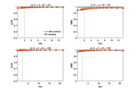
Figure 5: Classification results for CPL and K-means for DGP 1 ($K=2$) based on $L_{\tau}^{\prime}=D_{\tau}^{-1/2}AD_{\tau}^{-1/2}$. The $x$-axis marks the $\tau$ values and the $y$-axis is either CCP (left column) or NMI (right column). The green dashed vertical line in each subplot indicated the estimated $\tau^{\mathrm{JY}}$ value by using the method of Joseph and Yu (2016). The first and second rows correspond to $n/K=50$ and 200, respectively.

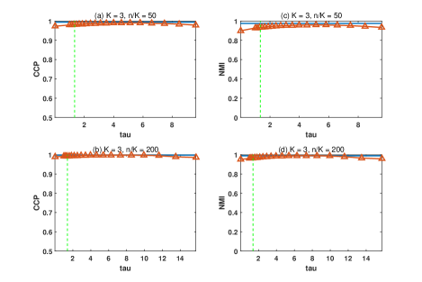
Figure 6: Classification results for DGP 2 ($K=3$) based on $L_{\tau}^{\prime}=D_{\tau}^{-1/2}AD_{\tau}^{-1/2}$. (See Figure 5 for explanations.)

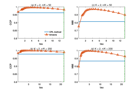
Figure 7: Classification results for DGP 3 ($K=2$, degree-corrected) based on $L_{\tau}=D_{\tau}^{-1/2}A_{\tau}D_{\tau}^{-1/2}$. (See Figure 5 for explanations.)

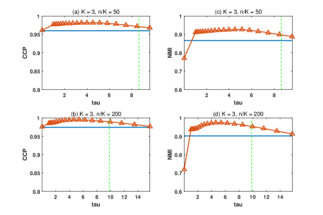
Figure 8: Classification results for DGP 4 ($K=3$, degree-corrected) based on $L_{\tau}=D_{\tau}^{-1/2}A_{\tau}D_{\tau}^{-1/2}$. (See Figure 5 for explanations.)

References

- Abbe (2018) Abbe, E., 2018. Community detection and stochastic block models: Recent developments. Journal of Machine Learning Research 18 (177), 1–86.
- Abbe et al. (2016) Abbe, E., Bandeira, A. S., Hall, G., 2016. Exact recovery in the stochastic block model. IEEE Transactions on Information Theory 62 (1).
- Abbe et al. (2017) Abbe, E., Fan, J., Wang, K., Zhong, Y., 2017. Entrywise eigenvector analysis of random matrices with low expected rank. arXiv preprint arXiv:1709.09565.
- Abbe and Sandon (2015) Abbe, E., Sandon, C., 2015. Community detection in general stochastic block models: Fundamental limits and efficient algorithms for recovery. In: Foundations of Computer Science (FOCS), 2015 IEEE 56th Annual Symposium on. IEEE, pp. 670–688.
- Ames (2014) Ames, B. P., 2014. Guaranteed clustering and biclustering via semidefinite programming. Mathematical Programming 147 (1-2), 429–465.
- Amini et al. (2013) Amini, A. A., Chen, A., Bickel, P. J., Levina, E., 2013. Pseudo-likelihood methods for community detection in large sparse networks. The Annals of Statistics 41 (4), 2097–2122.
- Bandeira et al. (2016) Bandeira, A. S., Boumal, N., Voroninski, V., 2016. On the low-rank approach for semidefinite programs arising in synchronization and community detection. In: Conference on learning theory. pp. 361–382.
- Bean et al. (2013) Bean, D., Bickel, P. J., El Karoui, N., Yu, B., 2013. Optimal m-estimation in high-dimensional regression. Proceedings of the National Academy of Sciences 110 (36), 14563–14568.
- Bickel and Chen (2009) Bickel, P. J., Chen, A., 2009. A nonparametric view of network models and Newman–Girvan and other modularities. Proceedings of the National Academy of Sciences 106 (50), 21068–21073.
- Bickel and Chen (2012) Bickel, P. J., Chen, A., 2012. Weak consistency of community detection criteria under the stochastic block model. Preprint.
- Bickel et al. (2011) Bickel, P. J., Chen, A., Levina, E., 2011. The method of moments and degree distributions for network models. The Annals of Statistics 39 (5), 2280–2301.
- Cai and Li (2015) Cai, T. T., Li, X., 2015. Robust and computationally feasible community detection in the presence of arbitrary outlier nodes. The Annals of Statistics 43 (3), 1027–1059.
- Chen and Lei (2017) Chen, K., Lei, J., 2017. Network cross-validation for determining the number of communities in network data. Journal of the American Statistical Association 0 (0), 1–11.
- Chen et al. (2014) Chen, Y., Jalali, A., Sanghavi, S., Xu, H., 2014. Clustering partially observed graphs via convex optimization. The Journal of Machine Learning Research 15 (1), 2213–2238.
- Chen et al. (2012) Chen, Y., Sanghavi, S., Xu, H., 2012. Clustering sparse graphs. In: Advances in neural information processing systems. pp. 2204–2212.
- Choi et al. (2012) Choi, D. S., Wolfe, P. J., Airoldi, E. M., 2012. Stochastic blockmodels with a growing number of classes. Biometrika 99 (2), 273–284.
- Chung (1997) Chung, F. R., 1997. Spectral graph theory. Vol. 92. American Mathematical Soc.
- Davis and Kahan (1970) Davis, C., Kahan, W. M., 1970. The rotation of eigenvectors by a perturbation. iii. SIAM Journal on Numerical Analysis 7 (1), 1–46.
- Hajek et al. (2016a) Hajek, B., Wu, Y., Xu, J., 2016a. Achieving exact cluster recovery threshold via semidefinite programming. IEEE Transactions on Information Theory 62 (5), 2788–2797.
- Hajek et al. (2016b) Hajek, B., Wu, Y., Xu, J., 2016b. Achieving exact cluster recovery threshold via semidefinite programming: Extensions. IEEE Transactions on Information Theory 62 (10), 5918–5937.
- Holland et al. (1983) Holland, P. W., Laskey, K. B., Leinhardt, S., 1983. Stochastic blockmodels: First steps. Social networks 5 (2), 109–137.
- Javanmard and Montanari (2015) Javanmard, A., Montanari, A., 2015. De-biasing the lasso: Optimal sample size for gaussian designs. arXiv preprint arXiv:1508.02757.
- Joseph and Yu (2016) Joseph, A., Yu, B., 2016. Impact of regularization on spectral clustering. The Annals of Statistics 44 (4), 1765–1791.
- Karrer and Newman (2011) Karrer, B., Newman, M. E., 2011. Stochastic blockmodels and community structure in networks. Physical Review E 83 (1), 016107.
- Lei (2016) Lei, J., 2016. A goodness-of-fit test for stochastic block models. The Annals of Statistics 44 (1), 401–424.
- Lei and Rinaldo (2015) Lei, J., Rinaldo, A., 2015. Consistency of spectral clustering in stochastic block models. The Annals of Statistics 43 (1), 215–237.
- Li et al. (2018) Li, X., Chen, Y., Xu, J., 2018. Convex relaxation methods for community detection. arXiv preprint arXiv:1810.00315.
- Lyzinski et al. (2014) Lyzinski, V., Sussman, D., Tang, M., Athreya, A., Priebe, C., 2014. Perfect clustering for stochastic blockmodel graphs via adjacency spectral embedding. Electronic Journal of Statistics 8 (2), 2905–2922.
- Mackey et al. (2014) Mackey, L., Jordan, M. I., Chen, R. Y., Farrell, B., Tropp, J. A., 2014. Matrix concentration inequalities via the method of exchangeable pairs. The Annals of Probability 42 (3), 906–945.
- Mossel et al. (2014) Mossel, E., Neeman, J., Sly, A., 2014. Consistency thresholds for binary symmetric block models. arXiv preprint arXiv:1407.1591 In proc. of STOC15.
- Newman and Girvan (2004) Newman, M. E., Girvan, M., 2004. Finding and evaluating community structure in networks. Physical review E 69 (2), 026113.
- Qin and Rohe (2013) Qin, T., Rohe, K., 2013. Regularized spectral clustering under the degree-corrected stochastic blockmodel. In: Burges, C. J. C., Bottou, L., Welling, M., Ghahramani, Z., Weinberger, K. Q. (Eds.), Advances in Neural Information Processing Systems. Vol. 26. Curran Associates, Inc., pp. 3120–3128.
- Rohe et al. (2011) Rohe, K., Chatterjee, S., Yu, B., 2011. Spectral clustering and the high-dimensional stochastic blockmodel. The Annals of Statistics 39 (4), 1878–1915.
- Sarkar and Bickel (2015) Sarkar, P., Bickel, P. J., 2015. Role of normalization in spectral clustering for stochastic blockmodels. The Annals of Statistics 43 (3), 962–990.
- Sussman et al. (2012) Sussman, D. L., Tang, M., Fishkind, D. E., Priebe, C. E., 2012. A consistent adjacency spectral embedding for stochastic blockmodel graphs. Journal of the American Statistical Association 107 (499), 1119–1128.
- Vershynin (2018) Vershynin, R., 2018. High-dimensional probability: An introduction with applications in data science. Vol. 47. Cambridge University Press.
- Vu (2018) Vu, V., 2018. A simple svd algorithm for finding hidden partitions. Combinatorics, Probability and Computing 27 (1), 124–140.
- Wang and Bickel (2017) Wang, Y., Bickel, P. J., 2017. Likelihood-based model selection for stochastic block models. The Annals of Statistics 45 (2), 500–528.
- Wilson et al. (2016) Wilson, J. D., Stevens, N. T., Woodall, W. H., 2016. Modeling and estimating change in temporal networks via a dynamic degree corrected stochastic block model. arXiv preprint arXiv:1605.04049.
- Yu et al. (2015) Yu, Y., Wang, T., Samworth, R. J., 2015. A useful variant of the Davis–Kahan theorem for statisticians. Biometrika 102 (2), 315–323.
- Yun and Proutiere (2014) Yun, S.-Y., Proutiere, A., 2014. Accurate community detection in the stochastic block model via spectral algorithms. arXiv preprint arXiv:1412.7335.
- Yun and Proutiere (2016) Yun, S.-Y., Proutiere, A., 2016. Optimal cluster recovery in the labeled stochastic block model. In: Advances in Neural Information Processing Systems. pp. 965–973.
- Zhao et al. (2012) Zhao, Y., Levina, E., Zhu, J., 2012. Consistency of community detection in networks under degree-corrected stochastic block models. The Annals of Statistics 40 (4), 2266–2292.
- Zhong and Boumal (2018) Zhong, Y., Boumal, N., 2018. Near-optimal bounds for phase synchronization. SIAM Journal on Optimization 28 (2), 989–1016.