High-Energy Variability of PSR J1311$-$3430

Abstract

We have studied the variability of the black-widow type binary millisecond pulsar PSR J1311$-$3430 from optical to gamma-ray energies. We confirm evidence for orbital modulation in the weak off-pulse $\stackrel{{\scriptstyle>}}{{{}_{\sim}}}$200-MeV emission, with a peak at $\phi_{B}\approx 0.8$, following pulsar inferior conjunction. The peak has a relatively hard spectrum, extending above $\sim 1$ GeV. XMM-Newton and Swift UV observations also show that this source’s strong X-ray flaring activity is associated with optical/UV flares. With a duty cycle $\sim 7-19$%, this flaring is quite prominent with an apparent power-law intensity distribution. Flares are present at all orbital phases, with a slight preference for $\phi_{B}=0.5-0.7$. We explore possible connections of these variabilities with the intrabinary shock and magnetic activity on the low mass secondary.

1. Introduction

“Black Widow”s (BWs) are energetic millisecond pulsars (MSPs) in short-period binaries driving a strong evaporative wind from their low-mass companion star. Optical observations of these companions often show the effect of this heating but in many cases the light curves do not match those expected from direct illumination by the pulsar (e.g. PSR J2215$+$5135; Schroeder & Halpern, 2014; Romani et al., 2015b). Instead, the heating power may be reprocessed in an intrabinary shock (IBS) set up between the relativistic pulsar wind and the massive wind driven from the companion (Romani & Sanchez, 2016). Thus the properties of this shock and its interaction with the companion star will be critical to understanding the evolution of BW MSPs.

Happily we see evidence for the wind in a range of other wavebands. In particular strong and variable radio eclipses of evaporating pulsars testify to an ionized plasma in the outflow. In a few cases (e.g. PSR J1311$-$3430; Romani et al., 2015a) we can see optical emission lines from atoms in the companion wind. At higher energies the relativistic shocked plasma in the IBS can contribute to strong orbital modulation in the X-ray band (Gentile et al., 2014), with caustic peaks due to beamed, likely synchrotron, emission. This high-energy emission is particularly valuable in helping map the geometry of the IBS. In addition, the variability of these systems from brief flares to the episodic accretion state changes of the so-called “transitioning” MSPs, such as PSR J1023$+$0038 (Archibald et al., 2009), gives important clues to the dynamics of the IBS.

We report here on the high-energy variability of an extreme member of this class, PSR J1311$-$3430 (hereafter J1311). With its $P_{b}=1.56$ hr orbital period (Romani, 2012) the shortest among confirmed MSPs (Pletsch et al., 2012) and a $\sim 0.01M_{\odot}$ He-rich companion indicating membership in the extreme “Tidarren” sub-class (Romani et al., 2016), this system has a particularly powerful IBS. It is also interesting as a possible high-mass neutron star and as a likely descendant of an Ultra-Compact X-ray Binary (UCXB) and progenitor of an isolated MSP. J1311 shows rich temporal variability, including claimed orbital modulation in off-pulse gamma rays (Xing & Wang, 2015) and rapid optical flares (Romani et al., 2015a). Here we study the orbital and short-period variabilities of J1311 for insights into the IBS physics and the companion heating, using Fermi Large Area Telescope (LAT; Atwood et al., 2009) data and archival optical and X-ray observations. In section 2, we describe the observational data we use. We show the analysis results in section 3. We then discuss and conclude in section 4.

2. Observational Data Sets and Basic Processing

We use $\sim$8 years of Fermi LAT (Atwood et al., 2009) data collected between 2008 August 04 and 2016 May 02 UTC, downloaded from the Pass-8 (Atwood et al., 2013) event archive and further analyzed with the Fermi-LAT Science Tools v10r0p5 along with P8R2_V6 instrument response functions. For our analyses, we use source class events with Front/Back event type in an $R=10^{\circ}$ aperture. We analyzed the 100 MeV–300 GeV and the 100 MeV–500 GeV data for the spectral and the timing analyses, respectively. We further employed standard $<90^{\circ}$ zenith angle and $52^{\circ}$ rocking angle cuts.

For X-ray data, we use archival Swift, Suzaku, XMM-Newton and Chandra observations. The Swift observations were made between MJD 54889 and 56731 and comprised 47 short observations. The total net Swift exposure is 90 ks. We processed the data using the XRT standard pipeline tools integrated with Heasoft 6.16 along with the HEASARC remote CALDB. Two Suzaku observations were taken in MJD 55047 (AO4, obs. ID 804018010, 40 ks) and MJD 55774 (AO6, obs. ID 706001010, 80 ks). We reprocessed the XIS data using the aepipeline tool in Heasoft 6.16. Results for analyses of these data have been reported previously (Romani, 2012; Kataoka et al., 2012). The XMM-Newton data were taken on MJD 56871 for 130 ks (obs. ID 0744210101). The EPIC data were processed using the epproc and the emproc tools in SAS version 20141104_1833. The archival Chandra data (Cheung et al., 2012; Arumugasamy et al., 2015) have exposures of 20 ks (Obs. ID 11790) and 10 ks (Obs. ID 13285), and are processed with chandra_repro in CIAO 4.7.2 to use the most recent calibration files.

For optical data, we use the archival Swift UVOT and XMM-Newton optical monitor observations. We processed these data using the uvotsource tool and the omichain tool, respectively. These were compared with ground-based light-curve studies (Romani et al., 2015a).

3. Data Analysis and Results

3.1. Fermi-LAT data analysis

We first performed a gamma-ray spectral analysis. We used a $R=10^{\circ}$ region of interest (RoI), and analyzed the data following the binned likelihood analysis as described in Fermi Science Support Center (FSSC). When fitting the data, we used a power-law with exponential cutoff model (PLEXP), $dN/dE=N_{0}(E/E_{0})^{-\Gamma_{\rm 1}}\mathrm{exp}(-(E/E_{\rm c})^{\Gamma_{\rm 2}})$, with $\Gamma_{\rm 2}$ held fixed at 1 for J1311 and fit all the bright sources ($\stackrel{{\scriptstyle>}}{{{}_{\sim}}}$5$\sigma$) in the aperture, the Galactic diffuse emission (gll_iem_v06.fits; Acero et al., 2016), and the isotropic diffuse emission (iso_P8R2_SOURCE_V6_v06.txt; Ackermann et al., 2015) in the 100 MeV–300 GeV band with pylikelihood. In the fit, we also include all the 3FGL sources within 20^∘ (Acero et al., 2015). We consider energy dispersion in the analysis, and therefore processed the data in the wider 60 MeV–500 GeV band. The best-fit parameters for J1311 are $\Gamma_{\rm 1}=1.87\pm 0.03\pm 0.04$, $E_{\rm c}=5.3\pm 0.5\pm 0.5$ GeV, with 100 MeV–300 GeV flux of $9.2\pm 0.3\pm 0.2\times 10^{-8}\rm\ phs\ cm^{-2}\ s^{-1}$ (see Table 1), consistent with the previous LAT spectral analysis within the uncertainties (Acero et al., 2015). The first and second uncertainties given for each parameter represent 1-$\sigma$ statistical and systematic uncertainties, respectively. Note that the systematic uncertainties are estimated by varying the scale for the response functions and normalization of the interstellar diffuse model (gll_iem_v06) by 6%. We then calculated changes in the best-fit parameters due to each systematic components and summed the errors in quadrature. We also varied the model; we hold all the parameters except for those of J1311 fixed at the 3FGL values or varied the number of sources to fit. We find that the results are all consistent with one another within the uncertainties. We further tried different RoI’s, $R=5^{\circ}$ and $R=15^{\circ}$, and performed similar studies. The results for these new RoI’s are also consistent with those for $R=10^{\circ}$ within the uncertainties.

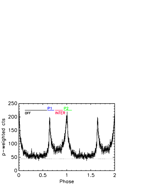
Figure 1.— Gamma-ray pulse profile (128 bins) in the 100 MeV–500 GeV and $R<2^{\circ}$. See section 2 for the timing solution. The phase-averaged background level estimated following Abdo et al. (2013) is shown with a dashed line.

Table 1Fit results for the orbital-phase averaged and orbital-phase revolved Fermi-LAT data in the “OFF” pulse-phase interval

Spin-phase resolved and orbital-phase averaged
Phase	$\Gamma_{\rm 1}$	$E_{\rm c}$	$F$
		(GeV)
ALL	$1.87\pm 0.03\pm 0.04$	$5.3\pm 0.5\pm 0.5$	$9.2\pm 0.3\pm 0.2$
P1	$1.71\pm 0.05\pm 0.06$	$4.7\pm 0.7\pm 0.4$	$14.5\pm 0.6\pm 1.4$
Inter	$1.67\pm 0.07\pm 0.11$	$3.7\pm 0.7\pm 0.6$	$8.1\pm 0.5\pm 1.3$
P2	$1.80\pm 0.04\pm 0.05$	$5.4\pm 0.8\pm 0.4$	$18.6\pm 0.6\pm 1.6$
OFF	$2.24\pm 0.12\pm 0.20$	$2.0\pm 0.7\pm 0.4$	$4.5\pm 0.3\pm 1.3$
Orbital-phase resolved in the “OFF” pulse-phase interval
Dip	$2.54\pm 0.11\pm 0.11$	$3.3\pm 0.0$	$4.3\pm 0.5\pm 1.2$
Hump	$2.33\pm 0.13\pm 0.19$	$3.3\pm 1.7\pm 0.6$	$5.2\pm 0.4\pm 1.3$

Notes. 1-$\sigma$ statistical and systematic uncertainties are shown.
^a100 MeV–300 GeV flux in units of $10^{-8}\ phs\rm\ cm^{-2}\ s^{-1}$.
^bHeld fixed at the best-fit value for the Hump spectrum (see Figure 2).

To isolate the strong gamma-ray pulsations, we checked the timing solution of Pletsch et al. (2012), folding the Fermi LAT events. These events were selected from small apertures ($R$$\stackrel{{\scriptstyle<}}{{{}_{\sim}}}$$2^{\circ}$). The source probabilities of each event, based on energy and position, were computed using gtsrcprob, and the time series was phased and folded using tempo2. Although the pulsar spin modulation shows very strongly, this solution, based on earlier LAT data, leaves a large drift in the pulse arrival time residual especially after MJD 56600. We therefore derived a new solution covering all data until MJD 57510.

Starting from the timing solution of Pletsch et al. (2012), we used the PINT software package and an unbinned Markov chain Monte Carlo maximum likelihood sampling technique (Sanpa-Arsa, 2016). We modeled the pulse profile using two asymmetric Lorentzians for the main peaks and a simple Gaussian for the bridge emission. The parameters of the template were varied jointly with the timing model parameters, allowing us to marginalize over the profile model. We found that accurately tracking the pulse phase required the addition of an orbital period derivative ($\dot{P}_{B}$), proper motion ($\mu_{\alpha}\mathrm{cos}\delta$ and $\mu_{\delta}$), and a second spin frequency derivative ($\ddot{\nu}$). Orbital eccentricity is undetected and fixed at $e=0$. The resulting best-fit parameters and their 1-$\sigma$ confidence intervals from the posterior distribution are reported in Table 2, and the resulting pulse profile appears in Figure 1.

Table 2Timing Parameters for PSR J1311$-$3430.

RA (J2000)	$13^{h}11^{m}45.72358(1)^{s}$
DEC (J2000)	$-34^{\circ}30^{\prime}30.342(3)^{\prime\prime}$
$\mu_{\alpha}\mathrm{cos}\delta$ (mas/yr)	$-$6.8(6)
$\mu_{\delta}$ (mas/yr)	$-$3.5(8)
Position Epoch (MJD)	56228
$\nu$ (s-1)	390.56839299885(1)
$\dot{\nu}$ (s-2)	$-$3.1882(3)$\times 10^{-15}$
$\ddot{\nu}$ (s-3)	1.03(8)$\times 10^{-25}$
Epoch (MJD)	56228
Binary model	ELL1
$P_{\rm B}$ (day)	0.0651157347(2)
$\dot{P}_{\rm B}$ ($s\ s^{-1}$)	3.7(3)$\times 10^{-12}$
Projected semi-major axis ($lt$-$s$)	0.010575(2)
$T_{\rm ASC}$ (MJD)	56009.129455(4)

^aSee Edwards et al. (2006) for the timing model definition.

Figure 2.— Off-pulse phase ($\Delta\phi_{P}$=0.127–0.587) orbital light curves taken with a $R<2^{\circ}$ aperture (MJD 54682–57510) for several different energy bands: (a) $E$=100 MeV–100 GeV, (b) $E$=200 MeV–1 GeV, (c) $E$=1 GeV–100 GeV. See Figure 1 for the off-pulse definition and section 2 for the timing solution. The phase-averaged background level estimated following Abdo et al. (2013) is shown with a dashed line.

By cutting on spin phase ($\phi_{P}$) to isolate the off-pulse region, one can minimize the pulsar magnetospheric flux and search for non-magnetospheric emission. In a study of 2,500 days of Pass-7 LAT data Xing & Wang (2015) found evidence for an orbital modulation of the off-pulse $>0.2$ GeV flux, finding $\sim$3$\sigma$ (0.003 chance probability) significance. To study such emission with our improved data set we constructed orbital light curves in the off- ($\phi_{P}=0.127-0.587$) and three on-pulse (P1, P2, and the interpulse, Figure 2) intervals. A concern for this study is that the orbital period $P_{b}\simeq 94$ mins is very close to that of the Fermi satellite (96 mins), hence artificial modulation may be produced due to the satellite’s orbital motion. We therefore folded time-resolved exposure ($\Delta T=30$ s) on the orbital period and confirmed that exposure variations across the phase bins used for the orbital light curves in Figure 2 were negligible ($\stackrel{{\scriptstyle<}}{{{}_{\sim}}}$1%). We also confirmed that varying zenith angle cuts to adjust the imperfect exclusion of Earth-limb gamma rays introduced no variation beyond the simple scaling due to changes in source count statistics.

As expected, no on-pulse interval shows significant modulation. However, the off-pulse light curves show modulation consistent with that reported by Xing & Wang (2015), deserving further study. Because we use a source-weighted photon analysis we did not need to use the very small apertures of that study. This avoids the extreme sensitivity of modulation significance to the aperture choice. With a conservative 2^∘ aperture, we compute the cumulative weighted H-test significance (Kerr, 2011) starting from the beginning or end of the data set; a significance which grows as more exposure is included indicates a real, steady signal. We track the modulation in low (200 MeV–1 GeV) and high (1 GeV–100 GeV) energy bands in addition to the full LAT range. The cumulative significance curves are shown in Figure 3, and the final low- and high-band light curves are shown in Figure 2. We further changed the aperture size (e.g., $R=3-5^{\circ}$) and found that the results do not change significantly. Although larger counts for larger apertures may result in higher significance especially at lower energies with the probability weighting, the weighting may not be accurate at the event-by-event level for timing analysis, hence an improvement in significance is not necessarily expected. As noted above the exposure variation rapidly becomes negligible, dropping to the percent level after $\sim$100 days of exposure. Monte Carlo simulations confirm that including this small variation in the bin exposure makes negligible difference to the H-test significance.

We note that the nearby flaring source 3FGL J1316.0$-$3338 (hereafter J1316) at a distance of $d\sim 1^{\circ}$ may affect the results. Although it is not very likely that this source exhibits periodic modulation on J1311 periods, a short-time flare of J1316 may be a concern. This effect is minimized because we use probability weighting, but there may be some residual effects. We therefore produced a light curve for J1316 and found two relatively large flares. We excised the time intervals for the these flares ($\pm 7$ days), and re-computed the H-test significance for J1311 in the three energy bands as we did above. We find that the results do not change whether or not we excise the J1316 flare intervals.

The low-band signal fades at late times while the high-band signal continues the secular increase in significance; this suggests some unknown, slowly varying, soft contamination. The full-band signal shows the largest significance, reaching $p\stackrel{{\scriptstyle<}}{{{}_{\sim}}}2\times 10^{-4}$. This significance decreases slightly, with $\sim 4.5\times 10^{-4}$ by the end of the data set; this is as expected since the low-band counts dominate. This $\sim 10\times$ improvement in significance over the Xing & Wang (2015) result is encouraging, but requires further exposure to be definitive. We can, of course, improve exclusion of low-energy and pulse contamination, by varying phase, aperture, time and energy cuts. As can be seen in Figure 1, using a narrower phase interval may suppress contaminations of the pulse peaks better and hence reveal stronger modulation. We therefore varied the selection criteria including the phase interval, and find the the results are not very sensitive to the selection criteria. For example, using $\phi_{p}=0.182-0.549$, aperture $R=1.27^{\circ}$, $E_{\gamma}$=1.01–100 GeV and interval MJD=56047–57431, we reach $p\sim 10^{-6}$ significance. Interestingly, this ‘tuned’ high-energy light curve is nearly 100% modulated. However, given that the post-trials significance is $\stackrel{{\scriptstyle>}}{{{}_{\sim}}}10^{-4}$, comparable to that for the initial un-tuned cuts, we cannot claim that such large modulation is required.

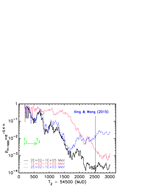
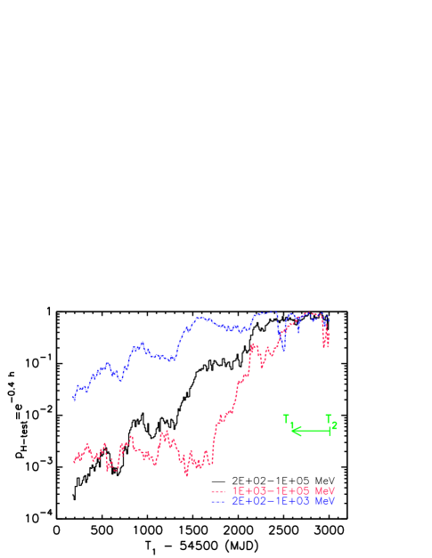
Figure 3.— Forward (left) and reverse (right) time-cumulative probabilities for the null hypothesis of a flat orbital light curve from the weighted counts shown in Figure 2. The time intervals for these plots are $T_{2}-T_{1}$, where for fixed $T_{1}=54682$, $T_{2}$ increases to 57510 (left), or for fixed $T_{2}=57510$, $T_{1}$ decreases to 54682 (right). Events are selected using an $R<2^{\circ}$ aperture, and each event is weighted by the probability. Three lines are for different energy bands: 200 MeV–100 GeV (black), 200 MeV–1 GeV (blue), and 1 GeV–100 GeV (red).

For phase-resolved spectral analysis, we generated the phase-resolved spectra for four different pulse-phase intervals: off-pulse (0.127–0.587), P1 (0.597–0.737), interpulse (0.757–0.917), and P2 (0.937–1.107) intervals, and performed likelihood analysis using pylikelihood with the data of each pulse interval. For these, normalizations for all the sources in the 3FGL model file were scaled down by the phase interval and the resulting flux for J1311 was scaled up by the same amount. The results are rather insensitive to the precise definition of these phase intervals. Here, we held all the parameters (except for those of PLEXP for J1311) fixed at the best-fit values obtained in the phase-averaged analysis above. The results are shown in Table 1. We further tried to see if the result changes if we fit the diffuse backgrounds (gll_iem_v06.fits and iso_P8R2_SOURCE_V6_v06.txt) as well, and found that the results do not change significantly.

For the off-pulse interval, we fit both the total flux and the spectra from the “hump” phase ($\phi_{B}=0.6-1.2$) and the lower “dip” phase ($\phi_{B}=0.2-0.6$). The spectral parameters are not significantly different although the hump power law is nominally slightly harder (Table 1). Note that the cutoff energy $E_{\rm c}$ for the “dip” phase is not well constrained, so we hold $E_{\rm c}$ at the value obtained for the “hump” phase. The spectra are shown in Figure 4 and the fit parameters are presented in Table 1. We have also fit a simple power-law (PL) model to the off-pulse phase spectra. Using the log-likelihood fit statistic, we find that PLEXP fits better than PL does with $\Delta\mathrm{l}og\mathcal{L}$ of 9, 1, and 7 for “all”, “dip”, and “hump”, respectively, in the 100 MeV–300 GeV band. For the “all” and the “hump” spectra, a curvature (i.e., a cutoff) is still required ($\stackrel{{\scriptstyle>}}{{{}_{\sim}}}$3$\sigma$), but we cannot tell whether the “dip” spectrum requires a curvature. Nevertheless, the shapes are very different from the on-pulse spectra (Fig. 4).

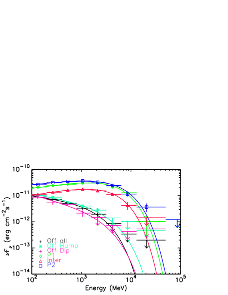
Figure 4.— Fermi-LAT SED of J1311. Flux in each energy band was measured by fitting the amplitude of the best-fit model (see Section 3.1) in that band. When the $TS$ value for the fit is less than 5, the 95% flux upper limit was derived by scanning the amplitude until log$\mathcal{L}$ changes by 1.35 with the UpperLimits.py script provided along with the Fermi-LAT Science Tools.

Because the low energy light curves’ significance appears concentrated in the early data, we also investigate long-term source variability. The variability index (Acero et al., 2015) in the 3FGL catalog is 52, and hence the total source flux has no significant variability. Variability might still be significant in some phase bins. As in section 3.1, we selected 4 phase intervals and constructed a light curve for each phase interval, with time bin 2 Ms for the faint off-pulse interval and 1 Ms for the rest. Note that there is a nearby variable source (J1316) which can contaminate the J1311 light curves. For each time bin, we performed likelihood analysis using pylikelihood to fit the amplitudes of J1311 and J1316. All other source and background parameters are held fixed at those obtained by a pulse-phase-resolved analysis (section 3.1). We used the best-fit source fluxes to calculate $\chi^{2}$ for a constant flux. As expected the on-pulse phases dominated by magnetospheric emission are consistent with steady flux. The off-pulse phase gives $\chi^{2}/{\rm dof}=57/86$, so even this interval is consistent with steady emission. We conclude that there is no long-term time variability in J1311, which is consistent with the study of Torres et al. (2017).

3.2. X-ray variability and Spectrum

J1311 is known to exhibit optical and X-ray flares (Romani, 2012; Kataoka et al., 2012), and a possible orbital modulation in the X-ray band has been reported (Kataoka et al., 2012; Arumugasamy et al., 2015). So a re-examination of the X-ray observations provides an important comparison with the gamma-ray modulation.

We re-examined archival X-ray observations taken with Swift, XMM-Newton and Suzaku. Source fluxes were extracted from apertures with radius $R=40^{\prime\prime}$, $R=16^{\prime\prime}$, and $R=40^{\prime\prime}$, respectively, while the background was monitored by nearby source-free apertures of radius $R=60^{\prime\prime}$, $R=32^{\prime\prime}$, and $R=60^{\prime\prime}$. Event times were barycentered with the ephemeris of section 3.1. In Figure 5 we plot the binned ($\Delta t=300$ s) XMM-Newton and Suzaku flux time series, with $t=0$ set at the ascending node prior to observation start. We use Chandra observations for spectral analysis only because of the short exposures and small number of counts. The source and background events are extracted using a $R=3^{\prime\prime}$ aperture and an annular region with $R_{\rm in}=5^{\prime\prime}$ and $R_{\rm out}=10^{\prime\prime}$, respectively.

We investigate source variability in the time series using the Bayesian block algorithm (Scargle, 1998; Scargle et al., 2013) implemented in the python astroML package (Vanderplas et al., 2012). The algorithm computes the number of optimal blocks and the change points for the time series. In the source time series, we find 15, 13, 5, 7, and 2 blocks for XMM-Newton, Suzaku/AO6, Suzaku/AO4, Swift, and Chandra; there are some blocks with much larger count rates than the minimum level and others similar to the minimum level (Figure 5). We performed the same analysis with the background time series to see if some of the source variabilities can be attributed to background activities. The Suzaku/AO4, Swift, Chandra backgrounds are well explained with a single block (i.e., no variability), and the others require 2–4 blocks suggesting some variability in the background; these variabilities are small and do not seem to correlate with the source activity. Furthermore, the background flux is only a small fraction of the source flux, hence the small background variabilities are unlikely to drive the source activities.

Strong flaring variability is clearly visible (Figure 5), with episodes reaching $>10\times$ the quiescent flux. We have marked some flux levels to help guide the eye at 4$\times$ the quiescent flux (red horizontal lines). There is no obvious preferred phase for flaring events. It appears, especially in the XMM-Newton data, that the flares can be clustered in episodes lasting several orbits $\sim 10-20$ ks.

The Swift data are snapshots over many years, so all we can show is the phase dependence of intervals (100–1400 s) where the flux was $>4\times$ the quiescence (Figure 5 e). In Figure 5 e, for only a few intervals was this excess more than 90% significant (red points in Figure 5 e). For the significance, we calculate the Poisson probabilities of having the observed counts in the time bins greater than the background plus $4\times$ the (XMM-estimated) quiescent counts, considering the trial factor (number of data bins in the figure). We denote these time bins in green lines in the Bayesian-block light curve as well (Figure 5 f). Two of the high-significance data points in Figure 5 e have a corresponding peak in Figure 5 f. The lowest one does not have a counterpart (green line at $T\approx 7\times 10^{4}$ s in Figure 5 f); this block has slightly elevated flux compared to the minimum, suggesting low level variability. In Figure 5 f, the first flare does not have a high-significance (red) counterpart in Figure 5 e; the corresponding point is denoted as a green cross in Figure 5 e. Again there is no clear phase grouping of the limited number of significant flares.

XMM-Newton has the highest count rate and the longest continued coverage. To test for orbital modulation we formed the light curve for “flare” ($T<56872.1$ MJD, the first $\sim$4 orbits in Figure 6 left) and “quiescent” ($T>56872.1$ MJD) periods (Figure 6 left) The quiescence light curve is fully consistent with constant flux ($p=0.5$); no variability is seen in our Bayesian-block analysis. With limited flare events in XMM alone the light curve is spiky, but we cannot discern a preferred phase. Substantially longer integrations are needed to infer the detailed flare behavior – but the data already show that flares can start at any phase.

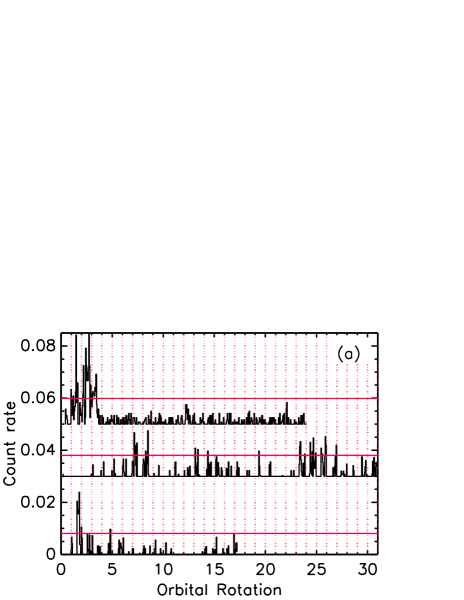
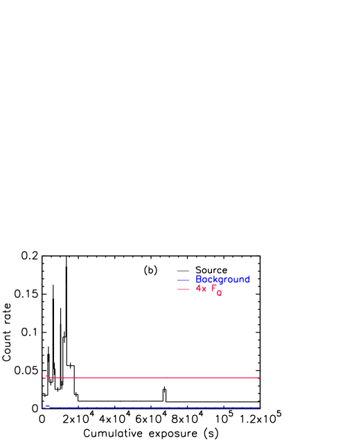
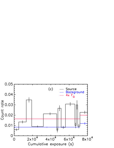
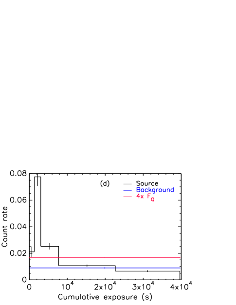
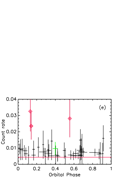
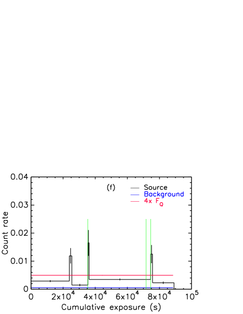
Figure 5.— (a): Unfolded 0.3–10 keV X-ray light curves of XMM-Newton/MOS, and Suzaku/XIS observations (300-s time bins, background subtracted). XMM-Newton, Suzaku AO6 and AO4 from the top. Data are offset, and amplitudes are scaled down by a factor of 4 (XMM-Newton) or 3 (Suzaku) for clarity. Red vertical lines mark phase 0. Note that the 96-minute Suzaku orbit is visible as gaps in the plot. (b)–(d): Bayesian-block representation of the light curves for the XMM-Newton (b), Suzaku/AO6 (c) and Suzaku/AO4 (d) data. Data gaps present in the data are removed in this representation to avoid artifacts produced due to the gaps (see Scargle et al., 2013). Backgrounds are shown in blue, and $4\times$ the quiescent level is shown in red. (e): A folded Swift light curve made of data points in which the flux is greater than $4\times$ the quiescent level. We denote data points which are significantly higher (with 90% confidence) than 4$\times$ the quiescent level in red. The green point corresponds to the first high-flux point in panel f. (f): Bayesian-block representation of the unfolded Swift light curve with the data gaps removed. Vertical green lines correspond to the high-flux points (red) in (e).

The XMM-Newton data provide by far the best statistics for measuring the X-ray spectrum. We can distinguish between the “flare” epoch and “quiescent” epochs. For each, we extracted source and background events using apertures of $R=16^{\prime\prime}$ and $R=32^{\prime\prime}$, respectively. We then calculated the response files using the standard tools of SAS version 20141104_1833 (rmfgen and arfgen). We then jointly fit the two 0.3–10 keV spectra with an absorbed power-law model having a common absorbing column density ($N_{\rm H}$). The source absorption is undetectably small; it is consistent with 0 with the current statistics. Unsurprisingly, the flare spectrum is substantially harder than that in quiescence (Table  3).

While other X-ray data sets provide insufficient statistics for accurate fits we can at least estimate fluxes and hardness. In all cases, we fix $N_{\rm H}=1\times 10^{20}\rm cm^{-2}$. For the Suzaku data we use $R=40^{\prime\prime}$ and $R=60^{\prime\prime}$ for the source and background apertures, respectively, and response files generated with XSELECT. The AO4 data had a clear bright flare and the separate flare and quiescence spectra have indices similar to the XMM measured values. In AO6 the source is relatively hard and bright when compared to the quiescent state observed with XMM-Newton, suggesting substantial flare contributions (Table 3; see also Figure 5 c). In the first of two archival CXO ACIS data sets the source is relatively bright with substantial flare contribution; the second is closer to quiescence. The spectral index uncertainties are too large to select a state. For Swift we simply combined all XRT observations, used pre-processed files for the source spectra and separately created background spectra using $R=60^{\prime\prime}$ apertures in the source-free regions. A fit to the merged spectrum gave an intermediate level average flux and a poorly determined, but hard $\Gamma$, again suggesting substantial contribution from poorly measured flares. Note that if the XMM flare/quiescence flux ratio is typical, a flare duty cycle as small as 10% will cause significant contamination in the spectral fits.

Table 3Absorbed Power Law Fits to the X-ray data

State	$N_{\rm H}$	$\Gamma$	$F_{\rm 0.3-10\,keV}$
	$10^{20}\rm cm^{-2}$	$\cdots$	$10^{-14}\rm erg\ cm^{-2}\ s^{-1}$
XMM flare	$1\pm 2\tablenotemark{a}$	$1.26\pm 0.07$	$47\pm 2$
XMM quiescence	$1\pm 2\tablenotemark{a}$	$1.67\pm 0.09$	$6.6\pm 0.3$
Suzaku AO4	$1\tablenotemark{b}$	$1.3\pm 0.1$	$26\pm 2$
Suzaku AO4 Flare	$1\tablenotemark{b}$	$1.19\pm 0.15$	$94\pm 10$
Suzaku AO4 Quie.	$1\tablenotemark{b}$	$1.6\pm 0.2$	$14\pm 2$
Suzaku AO6	$1\tablenotemark{b}$	$1.16\pm 0.05$	$40\pm 2$
Chandra 11790	$1\tablenotemark{b}$	$1.3\pm 0.3$	$18\pm 4$
Chandra 13285	$1\tablenotemark{b}$	$1.4\pm 0.3$	$8\pm 2$
Swift combined	$1\tablenotemark{b}$	$1.20\pm 0.15$	$19\pm 2$

^aTied.
^bFrozen.

3.3. Optical variability

The optical light curve has the dramatic $\sim 4$ magnitude ($\sim 40\times$) orbital modulation characteristic of BW pulsars, with maximum at pulsar inferior conjunction $\phi_{B}=0.75$ when the heated face of the companion is best visible. In addition it shows optical flares with rise times as short as $\sim 300$ s and amplitudes as large as $\sim 6\times$ the peak flux (Romani, 2012). We would like to know how these optical events relate to the X-ray flares above.

We are fortunate in having simultaneous optical data from the Swift/UVOT and XMM-Newton/Optical monitor (OM). Unfortunately, these data were taken with a variety of integration times and filters. The XMM-Newton/OM exposures were 2 ks ($\Delta\phi_{B}=0.36$). This coarse time sampling makes it difficult to identify any but the largest flares. The Swift/UVOT exposure varied between 30 s and 1.6 ks. To extract fluxes for an initial study of the optical behavior we used standard tools (uvotsource and omichain; Section 2). For the Swift data, we barycenter correct the exposure midpoint times. For the XMM-Newton data, we used the barycenter-corrected X-ray photon arrival times, and interpolate them to obtain the barycenter-corrected OM times. The omichain automatically detects the source in the XMM-Newton/OM data and properly calculates the source flux. For the Swift/UVOT data, we used a $R=5^{\prime\prime}$ and a $R=15^{\prime\prime}$ apertures for the source and the background, respectively, to measure the source flux.

The resulting barycentered midpoints of the Swift observations are phased with the binary ephemeris and plotted in Figure 6, with detections, mostly near $\phi_{B}=0.75$, in the first cycle and upper limits in the second cycle. To know if these detections are bright compared with the quiescent state we need to compare with the quiescent (pulsar heating) light curve. We can use the ground-based observations of Romani et al. (2015a) to interpolate quiescent $V$ and $B$ light curves. However the quiescent UV fluxes of J1311 are not known. The hot $T_{eff}\approx 12,000$ K face of the He companion must contribute some flux. However, after de-reddening by an estimated $E(B-V)=0.173$ (Galactic average towards J1311; Romani et al., 2015a), we find that the phase average optical UV spectrum does not match a simple blackbody. This is in contradiction to Kataoka et al. (2012)’s UVOT analysis.

Still, we need an estimate of the quiescent flux in the UV filters and so, to be conservative, we scaled the best-fit model $B$ light curve assuming a simple blackbody spectrum across the UVOT bands to generate $U$, $UVW1$, $UVM2$, and $UVW2$ light curves; these estimates are shown in Figure 6 and also consistent with the Swift upper limits. Note that the modest Swift $V$ sensitivity means that the source was only detected in a high (flare) state. One $B$ detection also likely represents a mild flare. In the $UVM2$ and $UVW2$ bands, the measured fluxes are in general higher than the blackbody-extrapolated model fluxes. This may suggest that the source spectrum at high frequencies deviates from a simple blackbody. Several UV detections during the ‘night’ phase ($\phi_{B}=0.0-0.5$) clearly represent a large increase over the expected quiescent flux. The XMM-Newton/OM data are very coarse and have few detections, yet we can identify several bright flare points here, as well.

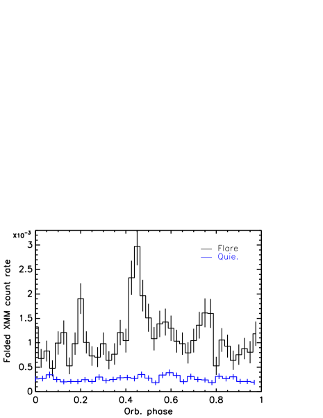
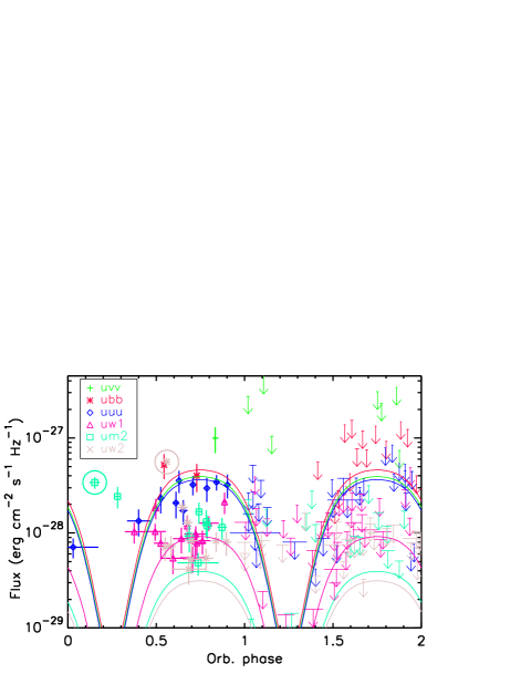
Figure 6.— Left: Folded X-ray orbital light curve measured with XMM-Newton/MOS during quiescence (blue, 113 ks) and flare (black, 20 ks). There are more events in the quiescent light curve due to the longer exposure. Right: Folded optical-band light curves measured with Swift/UVOT in the $V$, $B$, $U$, $UVW1$, $UVM2$, and $UVW2$ bands. Data points with error bars are for exposures in which J1311 is detected (first period). When the source is not detected, flux upper limit is shown (second cycle). Data points corresponding to the XRT high-flux states (red in Figure 5 e) are denoted with a circle.

3.4. Variability Statistics and the Optical/X-ray Correlation

We have identified flare intervals in each X-ray data set ($\Delta t\sim$300–400 s) for which the flux is $\stackrel{{\scriptstyle>}}{{{}_{\sim}}}4\times$ the quiescent value; adjacent flare bins are counted as a single flare. When finding the number of flares, we use the light curves made with constant time bins instead of the Bayesian-block representation because we are concerned with the gap removal; multiple flares separated by data gaps may be seen as one when the gap is removed. Note again that “flare” means the time intervals with measured flux greater than $4\times$ the quiescent level in our definition. We note that this definition for flare is arbitrary; we use this 4$\times$ the quiescent level only for reference flux (e.g., for “large” flux), and hence the “flare” definition should be considered with care. We then histogram the start phase of these flare events as a function of orbital phase (Figure 7). While it is clear that flares can be visible at any phase, with this coarse binning we see a mild, $\sim 50$% enhancement at and just before $\phi_{B}=0.75$, pulsar inferior conjunction when we view the heated face most directly. However, this excess has low ($p=$0.2) significance, and so additional monitoring will be needed to determine the flare phase distribution. Note that the difference in exposure time for each phase bin in Figure 7 is $\sim$10% (minimum to maximum), and has no significant impact. We show the exposure corrected flare counts in Figure 7.

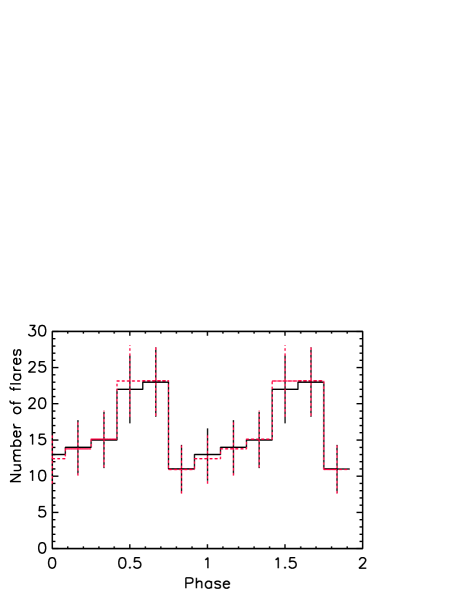
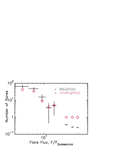
Figure 7.— Top: Number of flares detected in each phase in the X-ray observations (XMM-Newton, Suzaku, Swift combined). Red dashed line shows exposure-weighted flare counts. Bottom: Flux distribution of the detected flares. Black data points are made by weighting red points with the flux uncertainties.

We would like to know the duty cycle of this flaring activity. For this, we use the Bayesian block representation of the light curves (Figure 5 b–d and f). In the light curves, we calculate the count rates and the exposure times for each time bin. If we adopt the $>4\times$ flare definition then fully 19% of all intervals are in a flaring state. However, many of these must be statistically insignificant fluctuations. If we additionally require a 90% significance for the interval to have a flux excess using the Poisson statistic with the background and the XMM-estimated quiescent source flux, the flare duty cycle drops to 7%. Note that the duty cycle inferred this way is similar to what we infer using the binned light curves. We conclude that the true duty cycle at this $4\times$ threshold lies between these generous (19%) and conservative (7%) rates.

We also show the number of flares as a function of flux. In Figure 7 bottom, we plot the distribution of flare fluxes from all observations, with the flare flux in units of of the quiescent flux for the given observatory. Of course some excesses are low significance, and to account for this we also plot the flare flux weighted by the inverse of the flux uncertainties. This better approximates the true distribution, which is evidently a rather steep ($N\sim fl^{-3}$) power law.

Further, we can investigate the association of X-ray and optical flares of J1311. Because XMM-Newton and Swift provide simultaneous optical observations, data taken with these telescopes are particularly useful for this study. The OM data of XMM-Newton were taken only with the $V$ filter during the flare period, and we find that J1311 was detected only when the X-ray flaring activity is strongest. The OM time bins are of course large, but during the early bright flare $V$-band detections seem to span all phases, including ‘night’ phases. We thus infer that these $V$ detections are flare associated. The other OM filters were used during quiescence. The detections in these bands are only during the day phase, suggesting that we see only the heating modulation of the companion.

The many Swift observations allow us to plot the excess above background X-ray flux against the excess optical/UV flux beyond the heating model (Figure  8). The figure shows correlation between X-ray and optical fluxes. The significance of the linear correlation is 7$\sigma$ (although this is, of course, sensitive to the UV flux model that defines the flare excess). If we separately consider each band, the significance is highest in the $UVM2$ and the $UVW2$ bands, being $4\sigma$ and 5$\sigma$, respectively. We believe this suffices to show that the X-ray and optical/UV flares are due to the same events. Recently Halpern et al. (2017) have noticed correlated X-ray and optical variability in BW candidate XMMU J083850.38$-$282756.8, which may represent similar flaring events.

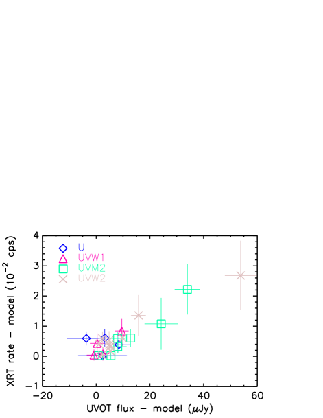
Figure 8.— UVOT flux vs. XRT count rates measured with Swift.

Finally, we would like to know if these X-ray/optical flare events are associated with the off-pulse GeV modulation shown in Figure 2. The low-significance modulation in Figure  7 peaks at the rising part of the off-pulse LAT light curve, so such association is at least plausible. However, we are unable to associate individual flare events with gamma-ray off-pulse activity. For $R<1^{\circ}$ from the source position, energy $>$1 GeV and pulse phase intervals of 0.127–0.587 we get a total count rate 0.17 day^-1, including background. However, the integrated flare time from all X-ray observations to date is 1.1 day. None of these gamma rays arrives during an X-ray flare, but the Poisson probability of this is 80%. In fact, given the substantial duty cycle for the flares, even if all off-pulse LAT photons arose during flare periods, we would expect $\sim 1$ coincident count. We attempted to boost the off-pulse count rate, by opening the energy range to $\stackrel{{\scriptstyle>}}{{{}_{\sim}}}$100 MeV (1.4 off-pulse photons/day), but this gives only 1.6 expected coincident counts (with a substantial fraction being background events). Two events are actually seen, no strong excess. Our only inference is that the Fermi-LAT flux during the X-ray flare intervals is $\stackrel{{\scriptstyle<}}{{{}_{\sim}}}$10$\times$ the quiescent flux (90% upper limit). Much more extensive (30–100d) X-ray or optical flare monitoring is needed to test for an event-level gamma-ray association. Thus we cannot make a direct connection and, for the foreseeable future, only an indirect connection of associated phase seems possible.

4. Discussion and Conclusions

We have analyzed optical to gamma-ray observations of J1311. As suggested by Xing & Wang (2015), orbital modulation seems to exist above 200 MeV in the off-pulse interval. Our analysis shows that the low-energy modulation ($\stackrel{{\scriptstyle<}}{{{}_{\sim}}}$1 GeV) weakens at later times ($p\approx 10^{-3}$ at 1600 days to $2\times 10^{-2}$ at 3000 days; the blue line in Figure 3 left) while high-energy ($>$1 GeV) modulation persists. This is puzzling because relative to the constant pulsar emission (Figure 4) the off-pulse emission is stronger at lower energies, hence larger modulation at lower energies is expected, which we do not see. However, if the modulation is driven by the bulk plasma motion in the IBS, stronger modulation in the high-energy band is possible because high-energy emission is produced only in limited phase intervals (e.g., An & Romani, 2017). Nevertheless, more data are required to establish firmly the gamma-ray modulation in J1311.

The overall off-pulse PLEXP spectral index $\Gamma_{\rm 1}=2.24$ is steeper than values seen for LAT MSPs (Abdo et al., 2013); thus is unlikely to be magnetospheric in origin, suggesting perhaps variable shock (likely IBS) emission.

The unpulsed source flux is maximum at the orbital phase $\sim$0.8 and minimum at $\sim$0.4 in the gamma-ray band (Figure 2 c). In massive star IBS (e.g. gamma-ray binaries) the observed gamma-ray modulation is believed to be primarily due to varying wind density (and hence shock stand-off, density and photon illumination) around an elliptical orbit. However, J1311 like other BW-type binaries has negligible eccentricity, and so the light curve peaks cannot be ascribed to orbital variation of the stars’ separation. Instead we must appeal to anisotropic emission and/or Doppler boosting in the relativistic post-shock flow.

In IBS emission models (e.g., An & Romani, 2017; Wadiasingh et al., 2017), particles are stochastically accelerated in the IBS formed by interaction between the neutron star’s wind and the companion’s wind, and flow along the contact discontinuity of the two winds. In addition, some particles can be adiabatically accelerated in the flow (e.g., Bogovalov et al., 2008). Hence, there can be both slow and fast (accelerated) populations in the shock. Both populations will emit synchrotron and inverse Compton radiation. Because of radiation reaction (competition between acceleration and energy loss of the emitting particles), the synchrotron photons emitted by the slow population can only reach energies of $\sim$160 MeV. The fast population’s bulk Lorentz factor can boost photons to higher energies. If the off-pulse emission is synchrotron radiation, this might explain the spectral variation, with the dip phase dominated by slower electrons and the hump including beamed, boosted emission from the fast population, with a spectral break pushed out above 200 MeV.

From the radio eclipses and optical emission lines, we see that the pulsar wind momentum flux exceeds that of the companion wind. Thus the IBS should wrap around the companion. In this case we expect a fast population’s synchrotron emission to be beamed along the shock limb, with a phase near $\phi_{B}\approx 0.25$. In contrast, if the off-pulse hump is primarily Compton emission, then we might expect a peak near $\phi_{B}\approx 0.75$ if optical photons from the heated face of the companion provide the seed population. This is a somewhat better match to the observed peak near $\sim 0.8$. Of course a more detailed model could account for this asymmetry since optical emission lines give good evidence that the companion wind is strongly swept back by orbital motion (e.g., Parkin & Pittard, 2008; Romani & Sanchez, 2016).

Unusually for a BW pulsar (e.g., Gentile et al., 2014; Arumugasamy et al., 2015) J1311 does not show any clear X-ray orbital modulation in quiescence. This is despite the fact that, with a photon index $\Gamma\sim 1.7$ it seems rather similar to other BW objects in its average emission. Also, most synchrotron or Compton models of the gamma-ray emission would predict similar modulation in the lower energy X-ray population. Perhaps it is then significant that the flare X-ray times appear unevenly distributed about the orbit. In this case we might assume that these optical/X-ray events provide the seed photons for gamma-ray Compton emission. Of course some portion of the unmodulated X-ray flux might be magnetospheric and a deep NuSTAR (Harrison et al., 2013) study might be able to find pulsations in this component.

Our connection between the optical and X-ray flares provides some insights into the nature of these events. In Romani et al. (2015a), a flare was observed spectroscopically, showing that, for that event at least, the optical emission arose from companion surface and that the energy deposition was well below the photosphere. The event peaked at phase $\phi_{B}\approx 0.85$ and covered a substantial fraction $\sim 30$% of the visible surface. The energy flux was two orders of magnitude higher than the pulsar flux at the orbital radius; we thus infer a rapid release of stored, likely magnetic, energy. Although this particular event had no X-ray coverage, it would be reasonable to expect that if the responsible magnetic field has a large coherence scale, penetrating the surface, then reconnection and particle acceleration above the photosphere could give rise to synchrotron emission producing the hard $\Gamma\sim 1.3$ X-ray events. If these flares seed the Compton upscattering by IBS-accelerated electrons, gamma-ray emission at similar phase would result. We note that these flares must not be directly connected with the pulsar heating since they can also be seen when looking toward the night face of the companion. A strong, companion-dynamo generated field might, however, be able to erupt at an any point on the companion surface. We note that similar correlated optical/X-ray flaring activity is found for many young stars (e.g., Feigelson et al., 2007). These authors find a similar power-law intensity distribution, but with somewhat smaller indices: 2–2.7. The average X-ray flare luminosity of the young M stars is typically $\sim 3\times 10^{29}{\rm erg\,s^{-1}}$. Using the pulsar DM distance of 1.4 kpc, the XMM flare luminosity and a 10% duty cycle J1311 has an average flare $L_{X}\approx 10^{31}{\rm erg\,s^{-1}}$; we can speculate this higher activity is related to the very short rotation period of the tidally locked companion star. Additional flare studies will be needed to pin down a phase preference, if any, and test this scenario. Improved, correlated studies with the X-ray events are needed to probe the emission physics and the extent of the radiating particle energy distribution.

The Fermi LAT Collaboration acknowledges generous ongoing support from a number of agencies and institutes that have supported both the development and the operation of the LAT as well as scientific data analysis. These include the National Aeronautics and Space Administration and the Department of Energy in the United States, the Commissariat à l’Energie Atomique and the Centre National de la Recherche Scientifique / Institut National de Physique Nucléaire et de Physique des Particules in France, the Agenzia Spaziale Italiana and the Istituto Nazionale di Fisica Nucleare in Italy, the Ministry of Education, Culture, Sports, Science and Technology (MEXT), High Energy Accelerator Research Organization (KEK) and Japan Aerospace Exploration Agency (JAXA) in Japan, and the K. A. Wallenberg Foundation, the Swedish Research Council and the Swedish National Space Board in Sweden.

Additional support for science analysis during the operations phase is gratefully acknowledged from the Istituto Nazionale di Astrofisica in Italy and the Centre National d’Études Spatiales in France. This work performed in part under DOE Contract DE-AC02-76SF00515.

H.A. acknowledges supports provided by the NASA sponsored Fermi Contract NAS5-00147 and by Kavli Institute for Particle Astrophysics and Cosmology (KIPAC). This research was supported by Basic Science Research Program through the National Research Foundation of Korea (NRF) funded by the Ministry of Science, ICT & Future Planning (NRF-2017R1C1B2004566). R.W.R. was supported in part by NASA grant NNX17AL86G.

References

- Abdo et al. (2013) Abdo, A. A., Ajello, M., Allafort, A., et al. 2013, ApJS, 208, 17
- Acero et al. (2015) Acero, F., Ackermann, M., Ajello, M., et al. 2015, ApJS, 218, 23
- Acero et al. (2016) —. 2016, ApJS, 223, 26
- Ackermann et al. (2015) Ackermann, M., Ajello, M., Albert, A., et al. 2015, ApJ, 799, 86
- An & Romani (2017) An, H., & Romani, R. W. 2017, ApJ, 838, 145
- Archibald et al. (2009) Archibald, A. M., Stairs, I. H., Ransom, S. M., et al. 2009, Science, 324, 1411
- Arumugasamy et al. (2015) Arumugasamy, P., Pavlov, G. G., & Garmire, G. P. 2015, ApJ, 814, 90
- Atwood et al. (2013) Atwood, W., Albert, A., Baldini, L., et al. 2013, ArXiv e-prints, arXiv:1303.3514
- Atwood et al. (2009) Atwood, W. B., Abdo, A. A., Ackermann, M., et al. 2009, ApJ, 697, 1071
- Bogovalov et al. (2008) Bogovalov, S. V., Khangulyan, D. V., Koldoba, A. V., Ustyugova, G. V., & Aharonian, F. A. 2008, MNRAS, 387, 63
- Cheung et al. (2012) Cheung, C. C., Donato, D., Gehrels, N., Sokolovsky, K. V., & Giroletti, M. 2012, ApJ, 756, 33
- Edwards et al. (2006) Edwards, R. T., Hobbs, G. B., & Manchester, R. N. 2006, MNRAS, 372, 1549
- Feigelson et al. (2007) Feigelson, E., Townsley, L., Güdel, M., & Stassun, K. 2007, Protostars and Planets V, 313
- Gentile et al. (2014) Gentile, P. A., Roberts, M. S. E., McLaughlin, M. A., et al. 2014, ApJ, 783, 69
- Halpern et al. (2017) Halpern, J. P., Bogdanov, S., & Thorstensen, J. R. 2017, ApJ, 838, 124
- Harrison et al. (2013) Harrison, F. A., Craig, W. W., Christensen, F. E., et al. 2013, ApJ, 770, 103
- Kataoka et al. (2012) Kataoka, J., Yatsu, Y., Kawai, N., et al. 2012, ApJ, 757, 176
- Kerr (2011) Kerr, M. 2011, ApJ, 732, 38
- Parkin & Pittard (2008) Parkin, E. R., & Pittard, J. M. 2008, MNRAS, 388, 1047
- Pletsch et al. (2012) Pletsch, H. J., Guillemot, L., Fehrmann, H., et al. 2012, Science, 338, 1314
- Romani (2012) Romani, R. W. 2012, ApJ, 754, L25
- Romani et al. (2015a) Romani, R. W., Filippenko, A. V., & Cenko, S. B. 2015a, ApJ, 804, 115
- Romani et al. (2015b) Romani, R. W., Graham, M. L., Filippenko, A. V., & Kerr, M. 2015b, ApJ, 809, L10
- Romani et al. (2016) Romani, R. W., Graham, M. L., Filippenko, A. V., & Zheng, W. 2016, ApJ, 833, 138
- Romani & Sanchez (2016) Romani, R. W., & Sanchez, N. 2016, ApJ, 828, 7
- Sanpa-Arsa (2016) Sanpa-Arsa, S. 2016, PhD thesis, University of Virginia, Charlottesville, VA, USA
- Scargle (1998) Scargle, J. D. 1998, ApJ, 504, 405
- Scargle et al. (2013) Scargle, J. D., Norris, J. P., Jackson, B., & Chiang, J. 2013, ApJ, 764, 167
- Schroeder & Halpern (2014) Schroeder, J., & Halpern, J. 2014, ApJ, 793, 78
- Torres et al. (2017) Torres, D. F., Ji, L., Li, J., et al. 2017, ApJ, 836, 68
- Vanderplas et al. (2012) Vanderplas, J., Connolly, A., Ivezić, Ž., & Gray, A. 2012, in Conference on Intelligent Data Understanding (CIDU), 47 –54
- Wadiasingh et al. (2017) Wadiasingh, Z., Harding, A. K., Venter, C., Böttcher, M., & Baring, M. G. 2017, ApJ, 839, 80
- Xing & Wang (2015) Xing, Y., & Wang, Z. 2015, ApJ, 804, L33