An Alternative Lattice Field Theory Formulation Inspired by
Lattice Supersymmetry -Summary of the Formulation-

Abstract

We propose a lattice field theory formulation which overcomes some fundamental difficulties in realizing exact supersymmetry on the lattice. The Leibniz rule for the difference operator can be recovered by defining a new product on the lattice, the star product, and the chiral fermion species doublers degrees of freedom can be avoided consistently. This framework is general enough to formulate non-supersymmetric lattice field theory without chiral fermion problem. This lattice formulation has a nonlocal nature and is essentially equivalent to the corresponding continuum theory. We can show that the locality of the star product is recovered exponentially in the continuum limit. Possible regularization procedures are proposed.The associativity of the product and the lattice translational invariance of the formulation will be discussed.

1 Introduction

We have been asking ourselves the following question: "If we stick to keeping exact supersymmetry (SUSY) on the lattice, what kind of lattice formulation are we led to ?" There have been several proposals but they have not been completely successful as general formulationsDondi:1976tx ; old-lattsusy ; D-W-lattsusy ; Kaplan2 ; Catterall1 ; Giedt3 ; Catterall3 ; Catterall4 ; Sugino ; Kato-Sakamoto-So2 ; DKKN ; Dadda-Kawamoto-Saito1 ; Damgaard-Matsuura ; Kikukawa-Nakayama ; Kadoh-Suzuki ; DAdda:2010hbr ; DAdda:2011drn . There are several difficulties towards exact lattice supersymmetry which are of fundamental nature and intertwined with each other and thus not easy to solve at the same time. In particular it is difficult to keep SUSY and gauge invariance exactly at the same time for all super charges. We find a possible answer to our question by introducing on the lattice a new type of product, the star product which is nonlocal in nature but recovers locality exponentially in the continuum limit. Our lattice formulation based on the star product turns out to be equivalent to the continuum theory and thus it still needs regularization as we shall discuss in the end. The details of the formulation is given in DAdda:2017bzo .

2 Difficulties of lattice SUSY and the possible solutions

Let us consider the simplest possible SUSY algebra in one dimension.

$$Q^{2}=i\partial$$ (1)

There are two fundamental difficulties in formulating exact SUSY on the lattice.
i) Breakdown of the Leibniz rule for the difference operator.
ii) Chiral fermion species doubler problem.
In order to establish SUSY algebra on the lattice it is natural to replace the derivative operator by a difference operator. There is however an ambiguity in choosing which difference operator we introduce among forward, backward, symmetric difference operators. We claim Hermiticity requires symmetric difference operator as the lattice difference operator. In other words the momentum representation of lattice translation generator should be real:

$$i\partial\psi(x)\rightarrow i\hat{\partial}\psi(x)\equiv i\frac{\psi(x+a)-\psi(x-a)}{2a}\rightarrow\frac{\sin ap}{a}\psi(p),$$ (2)

where $a$ is the lattice constant and $p$ is the lattice momentum. The symmetric difference operator satisfies the following shifted Leibniz rule for the product of two fields:

$$\hat{\partial}(\psi(x)\chi(x))=\hat{\partial}\psi(x)\chi(x-a)+\psi(x+a)\hat{\partial}\chi(x)=\hat{\partial}\psi(x)\chi(x+a)+\psi(x-a)\hat{\partial}\chi(x).$$ (3)

Eq.(3) shows the breaking of the Leibniz rule for the difference operator and this is inconsistent with the super algebra (1) if Leibniz rule is assumed for $Q$ on the lattice.

Naive fermion formulation on the lattice generates species doublers degree of freedom so the number of physical fermions will be increased compared to the number of bosons and this generates another source of SUSY breaking. In general this second difficulty ii) is considered to be a separate issue since chiral fermion problem for QCD is solved so that we may use the same method for the formulation of lattice SUSY. We, however, claim that exact SUSY on the lattice cannot be preserved unless the boson and fermion propagators have also on the lattice the simple relation ($D_{\hbox{bos}}=D_{\hbox{fer}}^{2}$) that they have in the continuum. Thus the second difficulty should be treated together with i). In fact we claim that the difficulties i) and ii) are fundamentally related. We need to solve these two difficulties at the same time.

It is natural to consider $i\hat{\partial}$ defined in (2) as a generator of lattice translation. As one can see it generates a two steps lattice translation. It is natural to consider that physical states should be the eigenstates of the lattice translation generator. One can easily recognize that simple eigenstates of the translation generator (2) are:

$$\psi=C,\leavevmode\nobreak\ \leavevmode\nobreak\ \leavevmode\nobreak\ \leavevmode\nobreak\ \leavevmode\nobreak\ \psi^{\prime}=C^{\prime}(-1)^{n},$$ (4)

where $C$ and $C^{\prime}$ are constant and $x=na$ (n: integer) is lattice coordinate. The alternating sign state corresponds to a high frequency part in momentum space and thus corresponds to a species doubler state. We claim that we need to introduce single lattice translation generator since the lattice constant is the minimum unit of translation. It is then natural to introduce half lattice structure to accommodate alternating sign state where now lattice coordinate is $x=na/2$. It is then a natural question: "What is the half lattice translation generator ?" From the SUSY algebra (1) it is most natural to identify that the half lattice translation is lattice SUSY transformation. In fact we found that this algebraic and geometrical correspondence works for lattice superfield where the alternating sign $(-1)^{\frac{2x}{a}}$ interchanges bosons and fermions and plays a crucial role in the SUSY transformationDAdda:2010hbr DAdda:2011drn .

For example in one dimension we introduce bosonic and fermionic lattice fields $\tilde{\Phi}(p)$ and $\tilde{\Psi}(p)$ in momentum representation to accommodate fermion species doublers and the bosonic counter parts to balance the degrees of freedom. We find the following $N=2$ SUSY transformation in one dimension:

$$Q_{1}\tilde{\Phi}(p)=i\cos\frac{ap}{4}\tilde{\Psi}(p),\leavevmode\nobreak\ \leavevmode\nobreak\ \leavevmode\nobreak\ \leavevmode\nobreak\ Q_{1}\tilde{\Psi}(p)=-4i\sin\frac{ap}{4}\tilde{\Phi}(p),$$

$$Q_{2}\tilde{\Phi}(p)=\cos\frac{ap}{4}\tilde{\Psi}\left(\frac{2\pi}{a}-p\right),\leavevmode\nobreak\ \leavevmode\nobreak\ \leavevmode\nobreak\ \leavevmode\nobreak\ Q_{2}\tilde{\Psi}\left(\frac{2\pi}{a}-p\right)=4\sin\frac{ap}{4}\tilde{\Phi}(p),$$ (5)

which satisfies the $N=2$ SUSY algebra:

$$Q_{1}^{2}=Q_{2}^{2}=2\sin\frac{ap}{2},\leavevmode\nobreak\ \leavevmode\nobreak\ \leavevmode\nobreak\ \leavevmode\nobreak\ \leavevmode\nobreak\ \leavevmode\nobreak\ \leavevmode\nobreak\ \leavevmode\nobreak\ \leavevmode\nobreak\ \leavevmode\nobreak\ \{Q_{1},Q_{2}\}=0,$$ (6)

where a dimensionless translation generator $2\sin\frac{ap}{2}$ is used here for simplicity. In this one dimensional $N=2$ model there are two fermions in the lattice field $\tilde{\Psi}(p)$; a particle state at $p=0$ and the species doubler at $p=\frac{2\pi}{a}$. In the boson sector we have corresponding counter part of fermions at each momentum region. In this way fermionic species doubler and their bosonic counter part constitute the super multiplet of $N=2$ SUSY algebraDAdda:2010hbr DAdda:2011drn . We consider this is one possible solution of the second problem: (A) The fermionic species doublers and the bosonic counterparts are identified as super partners.

As we can see in (5) we can construct the exact $N=2$ SUSY algebra in the momentum space. In constructing the action we impose SUSY invariance up to the surface terms. Cancellation of the surface terms in the coordinate space can be translated into the total momentum conservation in the momentum space. In order to keep the algebraic structure of SUSY exact in the momentum space it is natural to identify the momentum representation of the translation generator as the conserved momentum. In other words we replace the lattice momentum conservation with the conservation of a single lattice translation generator:

$$\delta(p_{1}+p_{2}+\cdots)\rightarrow\delta\left(\frac{2}{a}\sin\frac{ap_{1}}{2}+\frac{2}{a}\sin\frac{ap_{2}}{2}+\cdots\right).$$ (7)

It turns out that this replacement solves the difficulty of the lattice Leibniz rule i). This type of replacement was first suggested by Dondi and Nicolai in their pioneering work of lattice SUSY in Dondi:1976tx , where the conservation of a two step lattice translation generator $\frac{\sin ap}{a}$ was proposed. In our proposal we have introduced a half lattice structure to accommodate the geometric and algebraic correspondence of lattice SUSY transformationDAdda:2010hbr ; DAdda:2011drn .

If we express the product of two fields $\Phi_{1}(x)\cdot\Phi_{2}(x)$ in the momentum space this leads to a convolution of two fields:

$$\tilde{\Phi}_{1}(p)\cdot\tilde{\Phi}_{2}(p)=\frac{1}{2\pi}\int dp_{1}dp_{2}\delta(p-p_{1}-p_{2})\tilde{\Phi}_{1}(p_{1})\tilde{\Phi}_{2}(p_{2}).$$ (8)

If we replace the momentum conservation with (7) the product is changed from the normal product to a $\star$-product:

$$\tilde{\Phi}_{1}(p)\star\tilde{\Phi}_{2}(p)=\frac{1}{2\pi}\int dp_{1}dp_{2}\delta(\hat{p}-\hat{p}_{1}-\hat{p}_{2})\tilde{\Phi}_{1}(p_{1})\tilde{\Phi}_{2}(p_{2}),$$ (9)

where $\hat{p_{i}}=\frac{2}{a}\sin\frac{ap_{i}}{2}$. It is important to realize that the conservation of the lattice translation generator leads to the lattice Leibniz rule for the new $\star$-product:

$$\hat{p}(\tilde{\Phi}_{1}(p)\star\tilde{\Phi}_{2}(p))=\frac{1}{2\pi}\int dp_{1}dp_{2}\delta(\hat{p}-\hat{p}_{1}-\hat{p}_{2})(\hat{p}_{1}\tilde{\Phi}_{1}(p_{1})\tilde{\Phi}_{2}(p_{2})+\tilde{\Phi}_{1}(p_{1})\hat{p}_{2}\tilde{\Phi}_{2}(p_{2})),$$ (10)

where $\hat{p}_{i}=\frac{2}{a}\sin\frac{ap_{i}}{2}$ is nothing but a momentum representation of the difference operator.

By parametrizing the delta function in (9) we obtain the explicit presentation of the $\star$-product in coordinate space:

$$(\Phi_{1}\star\Phi_{2})\left(\frac{na}{2}\right)=\sum_{n_{1},n_{2}}K(n,n_{1},n_{2})\Phi_{1}\left(\frac{n_{1}a}{2}\right)\Phi_{2}\left(\frac{n_{2}a}{2}\right),$$ (11)

where

$$K(n,n_{1},n_{2})=\int^{\infty}_{-\infty}d\lambda J_{\Delta}\left(\lambda,\frac{na}{2}\right)J_{\Delta}\left(\lambda,\frac{n_{1}a}{2}\right)J_{\Delta}\left(\lambda,\frac{n_{2}a}{2}\right).$$ (12)

Here $J_{\Delta}$ is Bessel function:

$$J_{\Delta}\left(\lambda,\frac{na}{2}\right)=\frac{a}{2}\int^{\frac{4\pi}{a}}_{0}\frac{dp}{2\pi}e^{-i\left(n\frac{ap}{2}-\lambda\frac{a\Delta(p)}{2}\right)},$$ (13)

where $\Delta(p)=\hat{p}=\frac{2}{a}\sin\frac{ap}{2}$. As we can recognize the star product has a nonlocal nature.

If we express eq. (10) in coordinate space we can recognize that the single lattice translation difference operator satisfies exact Leibniz rule on the star product of fields, and thus the first difficulty i) is clearly solved. We can now construct actions of Wess-Zumino models for $N=2$ in one and two dimensions, which have exact lattice SUSY using the star product of fieldsDAdda:2010hbr DAdda:2011drn . In the one dimensional Wess-Zumino model species doublers of fermion and boson are identified as super multiplets of $N=2$ SUSY algebra. On the other hand in the two dimensional Wess-Zumino modelDAdda:2011drn chiral conditions require the truncation of species doubler degrees of freedom:

$$\tilde{\Phi}_{A}(p_{1},\cdots,p_{j},\cdots,p_{d})=\tilde{\Phi}_{A}(p_{1},\cdots,\frac{2\pi}{a}-p_{j},\cdots,p_{d}),\leavevmode\nobreak\ \leavevmode\nobreak\ \leavevmode\nobreak\ (j=1,\cdots,d),$$ (14)

where $A$ denotes both fermions and bosons and $d=2$ in two dimensions. In particular in the case of fermions we have identified the fermion with zero momentum and its species doubler $\left(p=\frac{2\pi}{a}\right)$. This is possible since species doubler has the same helicity as the one at the zero momentum due to the sign change of lattice momentum at $\frac{2\pi}{a}$:

$$\frac{d\Delta(p)}{dp}|_{p=0}=\frac{d\Delta(\frac{2\pi}{a}-p)}{dp}|_{p=\frac{2\pi}{a}}.$$ (15)

We identify this is the case (B) in contrast with (A): the identification of doublers as super partners.

It is interesting to recognize at this stage that the truncation of the species doubler d.o.f. of fermions and of their bosonic counter parts can be systematically realized by imposing the condition (14) irrespective of chiral conditions. In other words even for a non SUSY formulation we can eliminate the extra d.o.f. of fields by introducing the half lattice structure and by truncating species doubler d.o.f. in each direction of dimensions. This can be well understood if we look into the coordinate version of the truncation condition (14):

$$\Phi_{A}\left(\frac{n_{1}a}{2},\cdots,-\frac{n_{j}a}{2},\cdots,\frac{n_{d}a}{2}\right)=(-1)^{n_{j}}\Phi_{A}\left(\frac{n_{1}a}{2},\cdots,\frac{n_{j}a}{2},\cdots,\frac{n_{d}a}{2}\right),\leavevmode\nobreak\ \leavevmode\nobreak\ \leavevmode\nobreak\ (j=1,\cdots,d).$$ (16)

This condition also suggests that we only need to consider the first quadrant of coordinate space which has boundaries. This suggest naive breaking of lattice translational invariance of the formulation.

There may also appear a worry that the lattice translational invariance is lost by changing lattice momentum conservation to $\Delta(p)$ momentum conservation in (9). However the translational invariance of action is not lost but it is represented by infinitesimal transformations of the fields generated by $\Delta(p)$,

$$\delta_{\epsilon}\tilde{\varphi}_{A}(p)=\epsilon^{\mu}\Delta(p_{\mu})\tilde{\varphi}_{A}(p),$$ (17)

where $\epsilon_{\mu}$ is infinitesimal parameter.

We can thus conclude this section by remarking that the solution for the difficulties of lattice SUSY formulation i) and ii) have been obtained. The identification of the conserved momentum with the single lattice difference operator solves the Leibniz rule problem with the introduction of a new star product. The introduction of the half lattice structure accompanied by the truncation condition (14) solves the second problem.

3 Breakdown of associativity and its recovery in the star product

In order to formulate exact lattice SUSY it is enough to solve the difficulties i) and ii). In fact we found a formulation of the $N=2$ Wess-Zumino models in one and two dimensions which have exact SUSY on the latticeDAdda:2010hbr ; DAdda:2011drn . It has been also confirmed that SUSY on the lattice is preserved even at the quantum levelAsaka:2016cxm . It has, however, been recognized that associativity for the $\star$-product is broken:

$$(\tilde{\Phi}_{1}\star(\tilde{\Phi}_{2}\star\tilde{\Phi}_{3}))(p)$$

$$=\int dp_{23}\int dp_{1}\int dp_{2}\int dp_{3}\tilde{\tilde{\Phi}}_{1}(p_{1})\tilde{\tilde{\Phi}}_{2}(p_{2})\tilde{\tilde{\Phi}}_{3}(p_{3})\delta(\hat{p}_{23}-\hat{p}_{2}-\hat{p}_{3})\delta(\hat{p}-\hat{p}_{1}-\hat{p}_{23})$$

$$\neq\int dp_{12}\int dp_{1}\int dp_{2}\int dp_{3}\tilde{\tilde{\Phi}}_{1}(p_{1})\tilde{\tilde{\Phi}}_{2}(p_{2})\tilde{\tilde{\Phi}}_{3}(p_{3})\delta(\hat{p}_{12}-\hat{p}_{1}-\hat{p}_{2})\delta(\hat{p}-\hat{p}_{3}-\hat{p}_{12})$$

$$=((\tilde{\Phi}_{1}\star\tilde{\Phi}_{2})\star\tilde{\Phi}_{3})(p)$$ (18)

where $\hat{p}_{i}=\frac{2}{a}\sin\frac{ap_{i}}{2}$. This is because there is a region of phase space where the following domains (1) and (2) do not overlap:

$$(1) \leavevmode\nobreak\ \leavevmode\nobreak\ \leavevmode\nobreak\ |\hat{p}_{i}|<\frac{2}{a},\leavevmode\nobreak\ \leavevmode\nobreak\ |\hat{p}_{2}+\hat{p}_{3}|<\frac{2}{a},\leavevmode\nobreak\ \leavevmode\nobreak\ |\hat{p}_{1}+\hat{p}_{2}+\hat{p}_{3}|<\frac{2}{a}$$

$$(2) \leavevmode\nobreak\ \leavevmode\nobreak\ \leavevmode\nobreak\ |\hat{p}_{i}|<\frac{2}{a},\leavevmode\nobreak\ \leavevmode\nobreak\ |\hat{p}_{1}+\hat{p}_{2}|<\frac{2}{a},\leavevmode\nobreak\ \leavevmode\nobreak\ |\hat{p}_{1}+\hat{p}_{2}+\hat{p}_{3}|<\frac{2}{a}.$$ (19)

It is interesting to realize that the breakdown of associativity does not affect exact SUSY invariance on the lattice for non-gauge Wess-Zumino models. On the other hand the breakdown of the associativity for the $\star$-product makes it difficult to extend this formulation to gauge theories since associativity is crucial for the gauge invariance proof as we can see in the following example:

$$\Phi^{\dagger}(x)\star\Phi(x) \rightarrow(\Phi^{\dagger}(x)\star e^{-i\alpha(x)})\star(e^{i\alpha(x)}\star\Phi(x))$$

$$\neq\Phi^{\dagger}(x)\star(e^{-i\alpha(x)}\star e^{i\alpha(x)})\star\Phi(x)=\Phi^{\dagger}(x)\star\Phi(x).$$ (20)

In order to recover the associativity for the $\star$-product we notice that if momenta $\hat{p}_{i}$ does not have upper limit in (18); then $\frac{2}{a}$ is replaced by $\infty$ in (19) and associativity is recovered. For this reason we tried to find an alternative lattice translation generator $\Delta(p)$ with the following properties:

$$1)\leavevmode\nobreak\ \Delta(-p)=-\Delta(p),$$

$$2)\leavevmode\nobreak\ \frac{a}{2}\Delta(p)=\frac{ap}{2}+O\left(\left(\frac{ap}{2}\right)^{3}\right),$$

$$3)\leavevmode\nobreak\ \Delta(p)\leavevmode\nobreak\ \hbox{has to cover twice the whole real axis as}\leavevmode\nobreak\ p\leavevmode\nobreak\ \hbox{goes through the}\leavevmode\nobreak\ \frac{4\pi}{a}\leavevmode\nobreak\ \hbox{period.}$$

$$4)\leavevmode\nobreak\ \Delta(p)=\Delta\left(\frac{2\pi}{a}-p\right),\leavevmode\nobreak\ \leavevmode\nobreak\ \leavevmode\nobreak\ \lim_{p\rightarrow\pm\frac{\pi}{a}}\Delta(p)=\pm\infty.$$ (21)

We found an almost unique solution:

$$\hat{p}=\Delta_{G}(p)=\frac{1}{a}\log\frac{1+\sin\frac{ap}{2}}{1-\sin\frac{ap}{2}}.$$ (22)

This is the inverse Gudermannian function and it has the following nice expansion:

$$\frac{a}{2}\Delta_{G}(p)=2\left[\sin\frac{ap}{2}-\frac{1}{3}\sin\frac{3ap}{2}+\frac{1}{5}\sin\frac{5ap}{2}-\frac{1}{7}\sin\frac{7ap}{2}+\cdots\right],$$ (23)

which in coordinate representation is a sum over all odd half integer multiple of difference operators:

$$\Delta_{G}\Phi(x)=\frac{2}{a}\sum_{k=1}^{\infty}\frac{(-1)^{k+1}}{2k-1}\left[\Phi\left(x+\frac{(2k-1)a}{2}\right)-\Phi\left(x-\frac{(2k-1)a}{2}\right)\right],$$ (24)

and so it is intrinsically nonlocal in nature. In fig.1 we show plot of the inverse Gudermannian function

$$gd^{-1}(x)=\frac{1}{2}\log\frac{1+\sin x}{1-\sin x},$$ (25)

Figure 1: Plot of the Inverse Gudermannian function $gd^{-1}(x)$ in the fundamental interval $(-\pi,\pi)$

As we can see from the figure there is a species doubler at $x=\frac{ap}{2}=\pi$.

It is important to note that the condition 4) is crucial to keep the symmetry of the whole action under the equivalence of (14) together with the condition (15). In conclusion we have found a lattice field theory formulation which avoids all the difficulties to fulfill exact lattice SUSY:
i) Difference operator satisfies exact Leibniz rule on $\star$-product.
ii) No chiral fermion doublers by truncation of the doublers d.o.f.
iii) Associativity is satisfied for the $\star$-product.
It turns out that this nonlocal lattice field theory formulation is equivalent to the corresponding continuum theory. How comes that this is possible ?

Let us consider the normal product of two fields $\tilde{\Phi}_{1}(p)$ and $\tilde{\Phi}_{2}(p)$ which is expressed by a convolution in the momentum space:

$$\widetilde{\Phi_{1}\star\Phi_{2}}(\hat{p})=\frac{2}{\pi}\int_{\Delta_{G}(-\frac{\pi}{a})}^{\Delta_{G}(\frac{\pi}{a})}d\hat{p}_{1}d\hat{p}_{2}\tilde{\Phi}_{1}(\hat{p}_{1})\tilde{\Phi}_{2}(\hat{p}_{2})\delta\left(\hat{p}-\hat{p}_{1}-\hat{p}_{2}\right),$$ (26)

where $\hat{p}_{i}=\Delta_{G}(p_{i})$ and $\Delta_{G}(\pm\frac{\pi}{a})=\pm\infty$. The $\star$-product at this stage is the same as the normal product as it can be seen by simply changing the integration variables:

$$f(p)\frac{1}{f(p)}\frac{d\hat{p}}{dp}\widetilde{\Phi_{1}\star\Phi_{2}}(\hat{p}) = \frac{d\hat{p}}{dp}\frac{2}{\pi}\int_{-\frac{\pi}{a}}^{\frac{\pi}{a}}dp_{1}dp_{2}f(p_{1})$$ (27)

$$\frac{1}{f(p_{1})}\frac{d\hat{p_{1}}}{dp_{1}}\tilde{\Phi}_{1}(\hat{p}_{1})f(p_{2})\frac{1}{f(p_{2})}\frac{d\hat{p_{2}}}{dp_{2}}\tilde{\Phi}_{2}(\hat{p}_{2})\delta\left(\hat{p}-\hat{p}_{1}-\hat{p}_{2}\right).$$

This relation can be replaced by the following equivalent relation:

$$f(p)\leavevmode\nobreak\ \widetilde{\varphi_{1}\star\varphi_{2}}(p)=\frac{2}{\pi}\int_{-\frac{\pi}{a}}^{\frac{\pi}{a}}dp_{1}dp_{2}\frac{d\Delta_{G}(p)}{dp}f(p_{1})\tilde{\varphi}_{1}(p_{1})\leavevmode\nobreak\ f(p_{2})\tilde{\varphi}_{2}(p_{2})\delta\left(\Delta_{G}(p)-\Delta_{G}(p_{1})-\Delta_{G}(p_{2})\right),$$ (28)

where we identify the lattice wave function as:

$$\tilde{\varphi}_{i}(p_{i})=\frac{1}{f(p_{i})}\frac{d\Delta_{G}(p_{i})}{dp_{i}}\tilde{\Phi}_{i}(\Delta_{G}(p_{i})),\leavevmode\nobreak\ \leavevmode\nobreak\ \leavevmode\nobreak\ \leavevmode\nobreak\ \leavevmode\nobreak\ \leavevmode\nobreak\ \leavevmode\nobreak\ \leavevmode\nobreak\ \leavevmode\nobreak\ \leavevmode\nobreak\ \leavevmode\nobreak\ \leavevmode\nobreak\ \leavevmode\nobreak\ -\frac{\pi}{a}\leq p_{i}\leq\frac{\pi}{a}.$$ (29)

with $\hat{p}_{i}=\Delta_{G}(p_{i})$. As one can see from (29) the lattice field $\tilde{\varphi}(p_{i})$ is defined up to a renormalization factor $f(p_{i})$. The factor $\frac{d\Delta_{G}(p_{i})}{dp_{i}}=\frac{1}{{\cos\frac{ap}{2}}}$ plays a role of compensating the argument of delta function linear in $p$: $\delta(p-\cdots)$.

The fact that the lattice and the continuum fields may be related by eq.(29) and that under this correspondence the field product of the continuum theory becomes the star product (28) on the lattice is highly non trivial. It naturally raises the question: "Can the continuum and the lattice countable infinity have the same number of degrees of freedom ?" In other words: Can the continuum to lattice wave function relation be inverted ? We investigated this question in the coordinate space. It turned out that it is possible to make the correspondence invertible with a smooth continuum limit if we choose the function $f(p)$ as:

$$f(p)=\sqrt{\frac{d\Delta_{G}}{dp}}=\frac{1}{\sqrt{\cos\frac{ap}{2}}}.$$ (30)

The details of the arguments can be found in DAdda:2017bzo . The $\star$-product of lattice fields is then defined as:

$$\sqrt{\cos\frac{ap}{2}}\widetilde{\varphi_{1}\star\varphi_{2}}(p)=\frac{2}{\pi}\int^{\frac{\pi}{a}}_{-\frac{\pi}{a}}\frac{dp_{1}}{\sqrt{\cos\frac{ap_{1}}{2}}}\frac{dp_{2}}{\sqrt{\cos\frac{ap_{2}}{2}}}\tilde{\varphi}_{1}(p_{1})\tilde{\varphi}_{2}(p_{2})\int d\xi e^{i\xi(\Delta_{G}(p)-\Delta_{G}(p_{1})-\Delta_{G}(p_{2}))}.$$ (31)

The coordinate representation of the $\star$-product is given by

$$(\varphi_{1}\star\varphi_{2})^{(0)}(x_{n})=\frac{a^{2}}{4}\sum_{n_{1},n_{2}}K_{n,n_{1},n_{2}}\varphi^{(0)}_{1}(x_{n_{1}})\varphi^{(0)}_{2}(x_{n_{2}}),$$ (32)

where $(0)$ denotes the coordinate fields corresponding after the species doublers truncation. The kernel $K_{n,n_{1},n_{2}}$ is completely symmetric in the three indices and is given by

$$K_{n,n_{1},n_{2}}=\int_{-\infty}^{+\infty}d\xi\leavevmode\nobreak\ J^{(0)}_{\Delta_{G}}(\xi,x_{n})\leavevmode\nobreak\ J^{(0)}_{\Delta_{G}}(\xi,x_{n_{1}})\leavevmode\nobreak\ J^{(0)}_{\Delta_{G}}(\xi,x_{n_{2}}),$$ (33)

with

$$J^{(0)}_{\Delta_{G}}(\xi,x_{n})=\frac{1}{2\pi}\int_{-\frac{\pi}{a}}^{\frac{\pi}{a}}\frac{dp}{\sqrt{\cos\frac{ap}{2}}}e^{ix_{n}p-i\xi\Delta_{G}(p)},$$ (34)

where $x_{n}=\frac{na}{2}$.

Lattice to continuum and continuum to lattice transformation of fields in coordinate space are given by

$$\hskip 56.9055pt\leavevmode\nobreak\ \leavevmode\nobreak\ \leavevmode\nobreak\ \leavevmode\nobreak\ \leavevmode\nobreak\ \leavevmode\nobreak\ \leavevmode\nobreak\ \leavevmode\nobreak\ \leavevmode\nobreak\ \leavevmode\nobreak\ \leavevmode\nobreak\ \leavevmode\nobreak\ \leavevmode\nobreak\ \leavevmode\nobreak\ \leavevmode\nobreak\ \leavevmode\nobreak\ \leavevmode\nobreak\ \leavevmode\nobreak\ \leavevmode\nobreak\ \leavevmode\nobreak\ \Phi(\xi) = \frac{a}{2}\sum_{n}\leavevmode\nobreak\ J^{(0)}_{\Delta_{G}}(\xi,x_{n})\varphi_{0}(x_{n}),$$

$$\hskip 56.9055pt\leavevmode\nobreak\ \leavevmode\nobreak\ \leavevmode\nobreak\ \leavevmode\nobreak\ \leavevmode\nobreak\ \leavevmode\nobreak\ \leavevmode\nobreak\ \leavevmode\nobreak\ \leavevmode\nobreak\ \leavevmode\nobreak\ \leavevmode\nobreak\ \leavevmode\nobreak\ \leavevmode\nobreak\ \leavevmode\nobreak\ \leavevmode\nobreak\ \leavevmode\nobreak\ \leavevmode\nobreak\ \leavevmode\nobreak\ \leavevmode\nobreak\ \leavevmode\nobreak\ \varphi_{0}(x_{n}) = \int_{-\infty}^{\infty}d\xi\leavevmode\nobreak\ \bar{J}^{(0)}_{\Delta_{G}}(x_{n},\xi)\leavevmode\nobreak\ \Phi(\xi),$$ (35)

where

$$\bar{J}_{\Delta_{G}}^{(0)}(\eta,\xi)=J_{\Delta_{G}}^{(0)}(\xi,\eta)=\frac{N}{2\pi}\int_{-\frac{\pi}{2}}^{\frac{\pi}{2}}\frac{d\theta}{\sqrt{\cos(\theta)}}\leavevmode\nobreak\ e^{iN\left(\xi gd^{-1}(\theta)-\eta\theta\right)},$$ (36)

with $N=\frac{2}{a}$ and $gd^{-1}(\theta)$ is given in (25) and we have also replaced $x_{n}=\frac{na}{2}$ with the continuum variable $\eta$:

$$x_{n}=\frac{n}{N}\rightarrow\eta\leavevmode\nobreak\ \leavevmode\nobreak\ \leavevmode\nobreak\ (n\rightarrow\infty,\leavevmode\nobreak\ N\rightarrow\infty).$$ (37)

It is interesting to recognize that the arguments $\eta$ and $\xi$ are interchanged for $\bar{J}^{(0)}_{\Delta_{G}}$ and $J^{(0)}_{\Delta_{G}}$. This is similar to the Fourier transform and the inverse Fourier transform for $e^{ipx}$.

As we can see again the $\star$-product defined in (32) is nonlocal in nature. The first question here is: "Is the locality of the $\star$-product recovered in the continuum limit ?" The answer is "yes". We can show:

$$\lim_{N\rightarrow\infty}J^{(0)}_{\Delta_{G}}(\xi,\eta)=\delta(\xi-\eta).$$ (38)

See the details in DAdda:2017bzo . This assures the recovery of locality for the $\star$-product (32) in the continuum limit. The next question is "How much local is the $\star$-product ?" Here we show the explicit functional dependence of $J^{(0)}_{\Delta_{G}}(\xi=1,\eta)$ in fig.2.

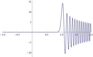
Figure 2: Plot of $J_{\Delta_{G}}^{(0)}(\xi=1,\eta)$ versus $\eta$ at $N=100$.

As we can see from the figure, around $\eta=1$ there is a peak, $\eta<1$ it decreases exponentially, $\eta>1$ it oscillates violently as an analytic continuation of exponential damping and thus plays a role of delta function. In fact damping nature below and above $\eta=1$ is thus exponential in nature. We can observe that the nonlocal $\star$-product is effectively local in the continuum limit.

We can now construct a continuum equivalent lattice field theory as follows:
(1) Write down the momentum representation of a continuum action.
(2) Replace the continuum derivative operator by $\Delta_{G}(p)$ and the lattice momentum conservation by the derivative operators conservation of $\Delta_{G}(p)$.
(3) Replace the continuum wave function by the lattice wave function as:

$$\tilde{\varphi}_{A}(p_{j})=\sqrt{\prod_{j}\frac{d\Delta_{G}(p_{j})}{dp_{j}}}\tilde{\Phi}_{A}(\hat{p}_{j})=\frac{1}{\sqrt{\prod_{j}\cos\frac{ap_{j}}{2}}}\tilde{\Phi}_{A}(\hat{p}_{j}).$$ (39)

(4) Identify all the fields as given in eq. (14) and consider only the first quadrant of coordinate space. We then obtain a continuum equivalent lattice action which has all the symmetries of the corresponding continuum theory and no chiral fermion problem. The $\star$-product is now associative.

All these replacements together with the substitution of (39) can be summarized in the following transformation from a continuum action to the corresponding lattice action:

$$e^{-\hat{S}_{\Delta_{G}}(\tilde{\varphi})}=\int\mathcal{D}\tilde{\Phi}_{A}\prod_{\mu}\prod_{p_{\mu}=-\frac{\pi}{a}}^{\frac{\pi}{a}}\prod_{A}\delta\left(\tilde{\Phi}_{A}(\Delta_{G}(p))-\sqrt{\prod_{j}\cos\frac{ap_{j}}{2}}\leavevmode\nobreak\ \tilde{\varphi}_{A}(p)\right)e^{-S_{cl}(\tilde{\Phi})}.$$ (40)

It is interesting to recognize that the transformation (39) can be identified as a momentum representation of block spin type transformation. A typical block spin type transformation from continuum to lattice can be given in the coordinate space as:

$$\varphi_{A}(n)=\int dxf(nl-x)\Phi_{A}(x),$$ (41)

where $f(nl-x)$ specifies blocking type. In this transformation the symmetries of the original action are not necessarily preserved. Criteria for the symmetries to be maintained on the lattice, at least in the Ginsparg-Wilson sense, were investigated in Bergner-Bruckmann . In our case, namely the blocking transformation (40) the symmetries of original theory are preserved in the lattice action.

There is, however, a crucial feature of this formulation namely that the lattice formulation is not yet regularized and the lattice constant is not playing the role of regulator. Nevertheless we have obtained a lattice field theory formulation which has the same lattice symmetries as the corresponding continuum theory have. We, however, need to regularize this lattice theory.

4 Regularization and renormalization in the new lattice

As a possible regularization we introduce regularization parameter $\hat{z}$ into the regularized derivative operator as:

$$\Delta^{(\hat{z})}_{G}(p)=\frac{1}{a\hat{z}}\log\frac{1+\hat{z}\sin\frac{ap}{2}}{1-\hat{z}\sin\frac{ap}{2}},$$ (42)

which extrapolates between two typical conserved momenta:

$$\lim_{\hat{z}\rightarrow 0}\Delta^{(\hat{z})}_{G}(p)=\frac{2}{a}\sin\frac{ap}{2},\leavevmode\nobreak\ \leavevmode\nobreak\ \leavevmode\nobreak\ \Delta^{(\hat{z}=1)}_{G}(p)=\Delta_{G}(p).$$ (43)

For $\hat{z}<1$ the regularized derivative operator $\Delta^{(\hat{z})}_{G}(p)$ is bounded by

$$|\Delta^{(\hat{z})}_{G}(p)|\leq\frac{1}{a\hat{z}}\log\frac{1+\hat{z}}{1-\hat{z}}=\hat{p}^{\hbox{(cutoff)}},$$ (44)

and thus plays a role of cut off momentum.

4.1 Wess-Zumino model in four dimensions

Let us consider as an example, the 4 dimensional Wess-Zumino model. The kinetic terms of the action are given by:

$$S=\int d^{4}x\left(i\Psi^{\dagger}\bar{\sigma}^{\mu}\partial_{\mu}\Psi-\partial^{\mu}\Phi^{\star}\partial_{\mu}\Phi\right),$$ (45)

where $(\bar{\sigma}^{\mu})=(\sigma^{0},-{\sigma}^{i})$. The action (45) is invariant on shell under the supersymmetry transformations:

$$\delta_{\epsilon}\Phi=\epsilon\Psi,\leavevmode\nobreak\ \leavevmode\nobreak\ \leavevmode\nobreak\ \leavevmode\nobreak\ \leavevmode\nobreak\ \leavevmode\nobreak\ \leavevmode\nobreak\ \leavevmode\nobreak\ \leavevmode\nobreak\ \leavevmode\nobreak\ \leavevmode\nobreak\ \leavevmode\nobreak\ \leavevmode\nobreak\ \leavevmode\nobreak\ \delta_{\epsilon}\Phi^{\star}=\epsilon^{\dagger}\Psi^{\dagger}$$ (46)

$$\delta_{\epsilon}\Psi_{\alpha}=-i(\sigma^{\mu}\epsilon^{\dagger})_{\alpha}\partial_{\mu}\Phi,\leavevmode\nobreak\ \leavevmode\nobreak\ \leavevmode\nobreak\ \leavevmode\nobreak\ \leavevmode\nobreak\ \leavevmode\nobreak\ \leavevmode\nobreak\ \leavevmode\nobreak\ \leavevmode\nobreak\ \leavevmode\nobreak\ \leavevmode\nobreak\ \leavevmode\nobreak\ \leavevmode\nobreak\ \delta_{\epsilon}\Psi^{\dagger}_{\dot{\alpha}}=i(\epsilon\sigma^{\mu})_{\dot{\alpha}}\partial_{\mu}\Phi^{\star},$$ (47)

and can be written in momentum representation:

$$S=\frac{1}{(2\pi)^{4}}\int d^{4}\hat{p}_{1}d^{4}\hat{p}_{2}\leavevmode\nobreak\ \delta^{4}\left(\hat{p}_{1}+\hat{p}_{2}\right)\left[-\tilde{\Psi}^{\dagger}(\hat{p}_{1})\bar{\sigma}_{\mu}\hat{p}_{2}^{\mu}\tilde{\Psi}(\hat{p}_{2})+\hat{p}_{1\mu}\tilde{\Phi}(\hat{p}_{1})\hat{p}_{2}^{\mu}\tilde{\Phi}^{\dagger}(\hat{p}_{2})\right],$$ (48)

where $\tilde{\Phi}^{\dagger}(\hat{p})$ is the Fourier transform of $\Phi^{\star}(x)$. As far as the kinetic terms of Wess-Zumino action are concerned the action (48) can be written on the lattice according to the previous sections’s prescriptions as

$$S^{(z)} = \frac{1}{\pi^{4}}\int_{-\frac{\pi}{a}}^{\frac{\pi}{a}}d^{4}p_{1}\leavevmode\nobreak\ d^{4}p_{2}\leavevmode\nobreak\ \prod_{\mu}\delta\left(p_{1\mu}+p_{2\mu}\right)\cdot$$ (49)

$$\cdot \left[-\tilde{\psi}^{\dagger}(p_{1})\bar{\sigma}^{\mu}\Delta_{G}^{(\hat{z})}(p_{2\mu})\tilde{\psi}(p_{2})+\Delta_{G}^{(\hat{z})}(p_{1\mu})\tilde{\varphi}(p_{1})\Delta_{G}^{(\hat{z})}(p_{2}^{\mu})\tilde{\varphi}^{\dagger}(p_{2})\right].$$

Here the regularized momentum operator is used for the derivative operators. We can show that this regularized lattice action is equivalent to the cut off version of the continuum action:

$$S^{(\hat{z})}=\frac{1}{(2\pi)^{4}}\int_{|\hat{p}_{\mu}|\leq\hat{p}^{(\mathrm{cutoff})}}d^{4}\hat{p}_{1}d^{4}\hat{p}_{2}\leavevmode\nobreak\ \delta^{4}\left(\hat{p}_{1}+\hat{p}_{2}\right)\left[-\tilde{\Psi}^{\dagger}(\hat{p}_{1})\bar{\sigma}_{\mu}\hat{p}_{2}^{\mu}\tilde{\Psi}(\hat{p}_{2})+\hat{p}_{1\mu}\tilde{\Phi}(\hat{p}_{1})\hat{p}_{2}^{\mu}\tilde{\Phi}^{\dagger}(\hat{p}_{2})\right],$$ (50)

with

$$\tilde{\Psi}(\Delta_{G}^{(\hat{z})}(p_{\mu}))=\frac{2\tilde{\psi}(p)}{\prod_{\mu}\sqrt{\frac{d\Delta_{G}^{(\hat{z})}(p_{\mu})}{dp_{\mu}}}}\leavevmode\nobreak\ \leavevmode\nobreak\ \leavevmode\nobreak\ \leavevmode\nobreak\ \leavevmode\nobreak\ \leavevmode\nobreak\ ,\leavevmode\nobreak\ \leavevmode\nobreak\ \leavevmode\nobreak\ \leavevmode\nobreak\ \leavevmode\nobreak\ \leavevmode\nobreak\ \tilde{\Phi}(\Delta_{G}^{(\hat{z})}(p_{\mu}))=\frac{2\tilde{\varphi}(p)}{\prod_{\mu}\sqrt{\frac{d\Delta_{G}^{(\hat{z})}(p_{\mu})}{dp_{\mu}}}}.$$ (51)

When the interaction terms are introduced the products are replaced by $\star$-product and the procedure goes quite parallel. SUSY is exactly kept on the lattice.

The action (50) is the action of a free theory in the continuum where a cutoff on the components of the momenta has been introduced. It is important to notice that in (50) the dependence on the lattice constant $a$ and the parameter $\hat{z}$, which was explicit in (49), is all contained in the value of $\hat{p}^{(\mathrm{cutoff})}$ which is given in (44). As a consequence lattice actions (49) with different values of the lattice constant $a$ and of the parameter $\hat{z}$ but corresponding to the same value of the cutoff $\hat{p}^{(\mathrm{cutoff})}$ according to eq. (44) are physically equivalent, as they correspond to the same continuum theory (50).

The conventional continuum action is reached by letting $\hat{p}^{(\mathrm{cutoff})}\rightarrow\infty$. This can be obtained in two ways, namely by either keeping $\hat{z}$ fixed (for instance $\hat{z}=0$) and taking the limit where the lattice spacing $a$ goes to zero (continuum limit), or by keeping the lattice spacing fixed and taking the limit $\hat{z}\rightarrow 1$. The lattice structure is preserved in the limit.

4.2 $\Phi^{4}$ theory in four dimensions

The lattice field theory formulation that we are proposing is completely general so that we can apply it also to non-SUSY field theories. Here we examine $\Phi^{4}$ theory. The momentum representation of $\Phi^{4}$ theory in four dimensions in the continuum is given by

$$S_{c} = \int d^{4}\hat{p}_{1}d^{4}\hat{p}_{2}\leavevmode\nobreak\ \delta^{(4)}(\hat{p}_{1}+\hat{p}_{2})\left[-\hat{p}_{1}^{\mu}\tilde{\Phi}(\hat{p}_{1})\hat{p}_{2\mu}\tilde{\Phi}(\hat{p}_{2})+m_{0}^{2}\tilde{\Phi}(\hat{p}_{1})\tilde{\Phi}(\hat{p}_{2})\right]$$ (52)

$$+ \lambda_{0}\int\prod_{i=1}^{4}d^{4}\hat{p}_{i}\leavevmode\nobreak\ \delta^{(4)}(\hat{p}_{1}+\hat{p}_{2}+\hat{p}_{3}+\hat{p}_{4})\leavevmode\nobreak\ \tilde{\Phi}(\hat{p}_{1})\tilde{\Phi}(\hat{p}_{2})\tilde{\Phi}(\hat{p}_{3})\tilde{\Phi}(\hat{p}_{4}),$$

The lattice version of this continuum expression can be obtained by replacing derivative operators and conserved momenta by the regularized lattice momentum $\hat{p}_{i\mu}=\Delta_{G}^{(\hat{z})}(p_{i\mu})$ and by replacing the continuum wave function by its lattice counterpart:

$$\tilde{\Phi}(\Delta_{G}^{(\hat{z})}(p_{\mu}))=\frac{2\tilde{\varphi}(p)}{\prod_{\mu}\sqrt{\frac{d\Delta_{G}^{(\hat{z})}(p_{\mu})}{dp_{\mu}}}}.$$ (53)

This essentially leads to a cut off theory of $\Phi^{4}$ theory in the momentum representation.

The introduction of the regulator $\hat{z}$ in the definition of the lattice derivative is not the only possible regularization procedure. Here we propose a different one, obtained by modifying the integration volume with the introduction of a parameter $\alpha$:

$$d^{4}\hat{p}_{1}\delta^{(4)}(\hat{p}_{1}+\cdots)\tilde{\Phi}(\hat{p}_{1})\rightarrow d^{4}{p}_{1}\delta^{(4)}({p}_{1}+\cdots)\left(\prod_{\mu=1}^{4}\frac{d\Delta_{G}(p_{i\mu})}{dp_{i\mu}}\right)^{2\alpha-1}\tilde{\varphi}(p_{1}).$$ (54)

The momentum representation of lattice $\Phi^{4}$ action can then be given by

$$S^{\alpha}=\int_{-\frac{\pi}{a}}^{\frac{\pi}{a}}d^{4}p_{1}d^{4}p_{2}\prod_{\mu=1}^{4}\delta(p_{1\mu}+p_{2\mu})\left[-\Delta_{G}(p_{1\mu})\Delta_{G}(p_{2\mu})+m_{0}^{2}\left(\prod_{\mu}\cos\frac{ap_{1\mu}}{2}\right)^{1-2\alpha}\right]\tilde{\varphi}(p_{1})\tilde{\varphi}(p_{2})$$

$$+\lambda_{0}\int_{-\frac{\pi}{a}}^{\frac{\pi}{a}}\prod_{i=1}^{4}d^{4}p_{i}\prod_{\mu=1}^{4}\delta\left(\sum_{i=1}^{4}\Delta_{G}(p_{i\mu})\right)\left(\prod_{i,\mu=1}^{4}\cos\frac{ap_{i\mu}}{2}\right)^{-\alpha}\tilde{\varphi}(p_{1})\tilde{\varphi}(p_{2})\tilde{\varphi}(p_{3})\tilde{\varphi}(p_{4}),$$ (55)

It is convenient also in this case to go back to the continuum representation, namely to use $\hat{p}_{i\mu}=\Delta_{G}(p_{i\mu})$ as independent momenta and $\Phi(\hat{p}_{i})$, defined in (53), as fundamental fields. With this change of variables we find:

$$S^{(\alpha)} = \int_{-\infty}^{\infty}d^{4}\hat{p}_{1}d^{4}\hat{p}_{2}\leavevmode\nobreak\ \delta^{(4)}(\hat{p}_{1}+\hat{p}_{2})\left[-\hat{p}_{1}^{\mu}\hat{p}_{2\mu}+\frac{m_{0}^{2}}{\left(\prod_{\mu}\cosh\frac{a\hat{p}_{1\mu}}{2}\right)^{1-2\alpha}}\right]\tilde{\Phi}(\hat{p}_{1})\tilde{\Phi}(\hat{p}_{2})$$ (56)

$$+ \lambda_{0}\int_{-\infty}^{\infty}\prod_{i=1}^{4}d^{4}\hat{p}_{i}\leavevmode\nobreak\ \delta^{(4)}(\hat{p}_{1}+\hat{p}_{2}+\hat{p}_{3}+\hat{p}_{4})\leavevmode\nobreak\ \frac{\tilde{\Phi}(\hat{p}_{1})\tilde{\Phi}(\hat{p}_{2})\tilde{\Phi}(\hat{p}_{3})\tilde{\Phi}(\hat{p}_{4})}{\left(\prod_{\mu}\prod_{i=1}^{4}\cosh\frac{a\hat{p}_{i\mu}}{2}\right)^{1/2-\alpha}}.$$

The kinetic term in (56) is the same as in the standard continuum theory, but the mass and the interaction terms are modified by the presence of the hyperbolic cosine factors which provide a smooth cutoff in the momenta: in fact for $\alpha<1/2$ each hyperbolic cosine denominator becomes very large for

$$\hat{p}_{i\mu}\gg\frac{1}{a(1/2-\alpha)}.$$ (57)

At one loop level the ultraviolet divergent diagrams are the one loop mass renormalization diagram, shown in fig.3, and the one-loop coupling renormalization diagrams illustrated in fig.4.

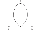
Figure 3: One-loop correction to the propagator.

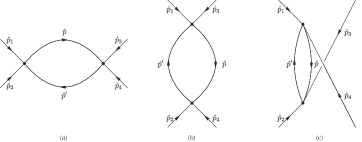
Figure 4: One-loop corrections to the four point vertex.

The propagator is given by

$$D^{(\alpha)}(\hat{p}_{1},\hat{p}_{2})=\frac{\prod_{\mu}\delta\left(\hat{p}_{1\mu}+\hat{p}_{2\mu}\right)}{\sum_{\mu}\hat{p}_{1}^{\mu}\hat{p}_{1\mu}+\left(\prod_{\mu}\cosh\frac{a\hat{p}_{1\mu}}{2}\right)^{2\alpha-1}m_{0}^{2}},$$ (58)

which turns into the following after one loop correction:

$$D_{1\textrm{loop}}^{(\alpha)}(\hat{p}_{1},\hat{p}_{2})=\frac{\prod_{\mu}\delta\left(\hat{p}_{1\mu}+\hat{p}_{2\mu}\right)}{\sum_{\mu}\hat{p}_{1}^{\mu}\hat{p}_{1\mu}+\left(\prod_{\mu}\cosh\frac{a\hat{p}_{1\mu}}{2}\right)^{2\alpha-1}\left(m_{0}^{2}+\lambda_{0}I_{\alpha}\right)},$$ (59)

where

$$I_{\alpha}=b_{2}\left(\frac{1}{a(1/2-\alpha)}\right)^{2}+b_{0}\leavevmode\nobreak\ m_{0}^{2}\log(1/2-\alpha)+\textrm{regular terms},.$$ (60)

Similarly coupling constant renormalization can be carried out:

$$\lambda_{0}\longrightarrow\lambda_{0}+\lambda_{0}^{2}\left(I_{\alpha}(\hat{p}_{1}+\hat{p}_{2})+I_{\alpha}(\hat{p}_{1}+\hat{p}_{3})+I_{\alpha}(\hat{p}_{3}+\hat{p}_{2})\right),$$ (61)

where

$$I_{\alpha}(\hat{p})=c_{0}\log(1/2-\alpha)+\textrm{regular terms}.$$ (62)

It is interesting to realize that the nonlocal nature of the lattice formulation is reflected as the momentum dependent mass term and coupling constant in the equivalent continuum theory. Nevertheless we can carry out renormalization procedure as in the standard treatment.

5 Conclusion and Discussions

We find a lattice formulation which is equivalent to the corresponding continuum theory. The problem of the species doubler d.o.f. for chiral fermions is consistently avoided. Explicit relations between continuum and lattice transformation of fields are derived and can be identified as a block spin type transformation. The reversibility of the transformation requires a special choice of lattice translation generator. The lattice formulation is nonlocal in nature but it recovers exponential locality in the continuum limit. All symmetries including lattice SUSY of the corresponding continuum theory can be kept exact, however, the regularized version still lacks associativity and thus lacks exact gauge invariance although it is assured to recover in the continuum limit.

It is worth to mention that the continuum-lattice duality introduced at the classical level by the reversible blocking transformation can be extended to the quantum level, and the lattice actions obtained in this way may be regarded as perfect actions Hasenfratz ; Bietenholz , with no lattice artifact in spite of finiteness of $a$.

It is a natural question if this lattice field theory formulation can be numerically feasible to carry out. The lattice field theory is nonlocal but all necessary expressions are well defined. Therefore we consider that numerical evaluation is in principle possible. The most naive regularization procedure for lattice regularization is to put the system in a box. Then the momentum is discretized then vanishing constraints of the continuum momentum $\Delta_{G}(p)$ in the delta function of (28) do not have a solution in generalBergner . This would cause another source of breaking symmetries. We can expect, however, that all the breaking effects would be negligible in the continuum limit since in the infinite box limit the lattice formulation is equivalent to the continuum theory.

In this approach lattice gauge theories and super Yang-Mills theories are still difficult to formulate in such a way that the gauge symmetry is strictly preserved. It could, however, be possible to evaluate the amount of breaking in the process of blocking transformation.

Acknowledgments

We thank P. H. Damgaard, I. Kanamori, H. B. Nielsen and Hiroshi Suzuki, for useful discussions over long years of our investigations. We also wish to thank JSPS and INFN for supporting our long standing collaboration.

References

• (1) P. H. Dondi and H. Nicolai, Nuovo Cim. A 41 (1977) 1.
• (2) S. Elitzur, E. Rabinovici and A. Schwimmer, Phys. Lett. B 199 (1982) 165.
T. Banks and P. Windey, Nucl. Phys. B198 (1982) 226.
N. Sakai and M. Sakamoto, Nucl. Phys. B229 (1983) 173.
J. Bartels and G. Kramer, ZPhys. C 20 (1983) 159.
S. Nojiri, Prog. Theor. Phys.  74 (1985) 819.
• (3) D. B. Kaplan, E. Katz and M. Ünsal, JHEP 0305 (2003) 037 [hep-lat/0206019].
A. G. Cohen, D. B. Kaplan, E. Katz and M. Ünsal, JHEP 0308 (2003) 024 [hep-lat/0302017]; JHEP 0312 (2003) 031 [hep-lat/0307012].
• (4) D.B. Kaplan, Nucl. Phys. Proc. Suppl. 129 (2004) 109, [arXiv:hep-lat/0309099].
• (5) S. Catterall, Nucl. Phys. Proc. Suppl. 129 (2004) 871, [arXiv:hep-lat/0309040].
• (6) J. Giedt, PoS LATTICE2006 (2006) 008, [arXiv:hep-lat/0701006].
• (7) S. Catterall, D.B. Kaplan and M. Ünsal, Phys. Rept. 484 (2009) 71, [arXiv:0903.4881[hep-lat]].
• (8) S. Catterall and S. Karamaov, Nucl. Phys. Proc. Suppl. 106 (2002) 935, [arXiv:hep-lat/0110071].
• (9) F. Sugino, JHEP 0401 (2004) 015 [arXiv:hep-lat/0311021]; JHEP 0403 (2004) 067, [arXiv:hep-lat/0401017]; JHEP 0501 (2005) 016, [arXiv:hep-lat/0410035].
• (10) M. Kato, M. Sakamoto and H. So, JHEP 05 (2008) 057, [arXiv:0803.3121 [hep-lat]], PoS LAT2005 (2006) 274, [arXiv:hep-lat/0509149].
• (11) A. D’Adda, I. Kanamori, N. Kawamoto and K. Nagata, Nucl. Phys. B 707 (2005) 100, [arXiv:hep-lat/0406029]; Nucl. Phys. Proc. Suppl. 140 (2005) 754, [arXiv:hep-lat/0409092]; Phys. Lett. B633 (2006) 645 [arXiv:hep-lat/0507029].
• (12) A. D’Adda, N. Kawamoto and J. Saito, Phys. Rev. D 81 (2010) 065001, [arXiv:0907.4137].
• (13) P. H. Damgaard and S. Matsuura, JHEP 0707 (2007) 051 [arXiv:0704.2696 [hep-lat]]; JHEP 0708 (2007) 087 [arXiv:0706.3007 [hep-lat]]; JHEP 0709 (2007) 097 [arXiv:0708.4129 [hep-lat]]; Phys. Lett.  B 661 (2008) 52 [arXiv:0801.2936 [hep-th]].
• (14) Y. Kikukawa and Y. Nakayama, PhysRevD66 (2002) 094508, [arXiv:hep-lat/0207013].
• (15) D. Kadoh and H. Suzuki, PhysLettB684 (2010) 167, [arXiv:hep-th/0909.3686].
• (16) A. D’Adda, A. Feo, I. Kanamori, N. Kawamoto and J. Saito, JHEP 1009 (2010) 059 doi:10.1007/JHEP09(2010)059 [arXiv:1006.2046 [hep-lat]].
• (17) A. D’Adda, I. Kanamori, N. Kawamoto and J. Saito, JHEP 1203 (2012) 043 [arXiv:1107.1629 [hep-lat]].
• (18) A. D’Adda, N. Kawamoto and J. Saito, arXiv:1706.02615 [hep-lat].
• (19) K. Asaka, A. D’Adda, N. Kawamoto and Y. Kondo, Int. J. Mod. Phys. A 31 (2016) no.23, 1650125 [arXiv:1607.04371 [hep-lat]].
• (20) G. Bergner, F. Bruckmann and J. M. Pawlowski, PhysRevD79 (2009) 115007.
• (21) P. Hasenfratz, NuclPhysB525 (1998) 401, [arXiv:hep-lat/9802007].
• (22) W. Bietenholz, Mod. PhysLettA14 (1999) 51.
• (23) G. Bergner, JHEP 1001 (2010) 024, [arXiv:hep-lat/0909.4791].