New results on disturbance rejection for energy-shaping controlled port-Hamiltonian systems

Abstract

In this paper we present a method to robustify energy-shaping controllers for port-Hamiltonian (pH) systems by adding an integral action that rejects unknown additive disturbances. The proposed controller preserves the pH structure and, by adding to the new energy function a suitable cross term between the plant and the controller coordinates, it avoids the unnatural coordinate transformation used in the past. This paper extends our previous work by relaxing the requirement that the systems Hamiltonian is strictly convex and separable, which allows the controller to be applied to a large class of mechanical systems, including underactuated systems with non-constant mass matrix. Furthermore, it is shown that the proposed integral action control is robust against unknown damping in the case of fully-actuated systems.

I INTRODUCTION

Port-Hamiltonian (pH) systems are a class of nonlinear dynamics that can be written in a form whereby the physical structure related to the system energy, interconnection and dissipation is readily evident [2]. Interconnection and damping assignment passivity-based control (IDA-PBC) is a control design that imposes a pH structure to the closed-loop dynamics [3]. This control method has been successfully applied to a range of nonlinear physical systems such as electrical machines [4, 5], power converters [6], chemical processes [7] and underactuated mechanical systems [8], [9]. Although IDA-PBC is robust to parameter uncertainty and passive preturbations, the presence of (practically unavoidable) external disturbances can significantly degrade its performance by shifting equilibria or even causing instability. In this paper, we focus on the problem of robustifying IDA-PBC vis-à-vis external disturbances via the addition of integral action control (IAC).

A number of IACs have been proposed for pH systems, each conforming to specified control objectives. In [3], an integrator is applied to the passive output of a pH system which has the effect of regulating the passive output to zero. This scheme can be interpreted as a control by interconnection (CbI), studied in [17], and is robust against parameters of the open-loop plant. A fundamentally different approach was taken in [11, 12] where the control objective was to regulate a signal that is not necessarily a passive output of the plant. As such, it was shown that the IAC for passive outputs proposed in [3] was not applicable as it cannot be implemented in a way that preserves the pH form. Rather, a partial state transformation was utilised to ensure that the closed-loop dynamics preserve the pH form. A critical step in this approach is the evaluation of the systems energy function at the transformed coordinates, which is a rather unnatural construction—see Remark 2 in [14]. This IAC was tailored for fully-actuated mechanical systems in [13] and underactuated mechanical systems in [14]. While in both cases the required change of coordinates to preserve the pH form were given explicitly, a number of technical assumptions were imposed to do so in the underactuated case. In both cases, the proposed IACs were shown to preserve the desired equilibrium of the system, rejecting the effect of an unknown matched disturbance.

More recently, an alternate approach to IAC design for pH systems was proposed in [15, 16]. The IAC is designed, as in [11, 12], to regulate signals that are not necessarily passive outputs of the plant. The key advancement over previous solutions is that the IAC does not require any coordinate transformations in the design procedure. Rather, the energy function of the controller depends on both the states of the controller and the plant which allows preservation of the pH structure by construction. It has been shown in [16] that the closed-loop can be interpreted as the power preserving interconnection of the plant and controller, which resembles the CbI technique [17]. It was also shown that, under a number of technical assumptions, the IAC could reject the effects of both a matched and unmatched disturbance.

In this paper, the realm of application of the IAC presented in [16] is significantly extended by relaxing some previously made assumptions. Specifically, the assumption in [16] that the open-loop Hamiltonian is strongly convex and separable is not required here. By relaxing this assumption, our result can be applied to a broader class of pH system. In particular, our result applies to a strictly larger class of underactuated mechanical systems than the ones considered in [14] and [16].

The remainder of the paper is structured as follows: The problem formulation is presented in Section II. A brief summary of previous work is given in Section III. The new IAC scheme is presented in Section LABEL:ia and the stability properties of the closed-loop are considered in Section LABEL:sec5. The IAC is tailored for mechanical systems in Section VI. The control scheme is applied to three examples in Section VII. Finally, the results of the paper are briefly discussed in Section VIII.

Notation. Function arguments are declared upon definition and are omitted for subsequent use. For $x\in\mathbb{R}^{n}$ we define $|x|^{2}=x^{\top}x$ and $\|x\|^{2}_{P}=x^{\top}Px$, for $P\in\mathbb{R}^{n\times n}$, $P>0$. All functions are assumed to be sufficiently smooth. For mappings $\mathcal{H}:\mathbb{R}^{n}\to\mathbb{R}$, $\mathcal{C}:\mathbb{R}^{n}\to\mathbb{R}^{m}$ and $\mathcal{G}:\mathbb{R}^{p}\times\mathbb{R}^{s}\to\mathbb{R}$ we denote the transposed gradient as $\nabla\mathcal{H}:=\left(\frac{\partial\mathcal{H}}{\partial x}\right)^{\top}$, the transposed Jacobian matrix as $\nabla{\cal C}:=\left(\frac{\partial\mathcal{C}}{\partial x}\right)^{\top}$ and $\nabla_{x}\mathcal{G}(x,y):=\left(\frac{\partial\mathcal{G}}{\partial x}\right)^{\top}$. For the distinguished $x^{\star},\bar{x}\in\mathbb{R}^{n}$, we define the constant vectors $\bar{\cal C}:={\cal C}(\bar{x}),\;{\cal C}^{\star}:={\cal C}(x^{\star})$, $\nabla\mathcal{H}^{\star}:=\nabla\mathcal{H}(x^{\star})$ and $\nabla\bar{\mathcal{H}}:=\nabla\mathcal{H}(\bar{x})$.

II Problem formulation

II-A Perturbed system model

In this paper we consider the scenario where an unperturbed system has been stabilised at a desired constant equilibrium using IDA-PBC and the objective is to add an IAC to reject additive disturbances. More precisely, the dynamics of the system are of the form:

$$\begin{bmatrix}\dot{x}_{a}\\ \dot{x}_{u}\end{bmatrix} = [J(x)-R(x)]\begin{bmatrix}\nabla_{x_{a}}\mathcal{H}\\ \nabla_{x_{u}}\mathcal{H}\end{bmatrix}+\begin{bmatrix}u-d_{a}(x)\\ -d_{u}(x)\end{bmatrix}$$

$$y_{a} = \nabla_{x_{a}}\mathcal{H}$$

$$y_{u} = \nabla_{x_{u}}\mathcal{H},$$ (1)

where $x=\operatorname{col}(x_{a},x_{u})\in\mathbb{R}^{n}$ is the state vector, with $x_{a}\in\mathbb{R}^{m}$ and $x_{u}\in\mathbb{R}^{s}$, $s:=n-m$, the actuated and unactuated states, respectively, $y_{a}\in\mathbb{R}^{m}$, $y_{u}\in\mathbb{R}^{s}$ are the signals to be regulated to zero and $u\in\mathbb{R}^{m}$ is the control input. The function $\mathcal{H}:\mathbb{R}^{n}\to\mathbb{R}_{+}$ is the Hamiltonian of the system. The interconnection and damping matrices are partitioned as

$$\begin{split}J(x):=\begin{bmatrix}J_{aa}(x)&J_{au}(x)\\ -J_{au}^{\top}(x)&J_{uu}(x)\end{bmatrix}&=-J^{\top}(x)\\ R(x):=\begin{bmatrix}R_{aa}(x)&R_{au}(x)\\ R_{au}^{\top}(x)&R_{uu}(x)\end{bmatrix}&=R^{\top}(x)\geq 0,\end{split}$$ (2)

respectively. The signals $d_{a}:\mathbb{R}^{n}\to\mathbb{R}^{m}$ and $d_{u}:\mathbb{R}^{n}\to\mathbb{R}^{s}$ are the, state-dependent, matched and unmatched disturbances of the system, respectively.

We assume that the energy-shaping and damping injection steps of the IDA-PBC design have been accomplished for system (1). This means, on one hand, that a desired equilibrium $x^{\star}\in\mathbb{R}^{n}$ satisfies

$$x^{\star}=\arg\min{\cal H}(x)$$

and is isolated, which implies that the system (1) without disturbances and $u=0_{m\times 1}$ has a stable equilibrium at $x^{\star}$. On the other hand, the damping injection step—consisting of a proportional feedback around the passive output—ensures that

$$-\nabla^{\top}{\cal H}\;R\;\nabla{\cal H}\leq-\alpha|y_{a}|^{2},$$

and $\alpha>0$ is a constant. Consequently, the equilibrium is asymptotically stable if $y_{a}$ is a detectable output for the system. See [21] for further details on stability of pH systems.

Notice that we have taken the input matrix of the form $\begin{bmatrix}I_{m}\\ 0_{s\times m}\end{bmatrix}$. As is well-known [1] a necessary and sufficient condition to transform—via input and state changes of coordinates—an arbitrary input matrix into this form is that its columns span an involutive distribution.

II-B Assumptions

As indicated in the introduction the objectives of the IAC are to preserve the existence of a stable equilibrium and to ensure that the output signal ($y_{a}$ and $y_{u}$ when $d_{u}=0_{s\times 1}$ or $y_{u}$ if $d_{a}=0_{m\times 1}$) is driven to zero in spite of the presence of disturbances. Also, some stability properties should be preserved when both disturbances act simultaneously. In this subsection we present the assumptions that are imposed on the system (1) to attain these objectives.

For the case of matched disturbances it is possible to preserve in closed-loop the original equilibrium $x^{\star}$. This, clearly, implies that if this equilibrium is asymptotically stable then $|y_{a}(t)|\to 0$, $|y_{u}(t)|\to 0$ as desired. In order to ensure the former property for state-dependent disturbances the following assumption is imposed.

Assumption 1

The disturbance $d_{a}$ can be written in the form

$$d_{a}=G_{d}(x)\bar{d}_{a},$$

where $\bar{d}_{a}\in\mathbb{R}^{m}$ is constant and $G_{d}:\mathbb{R}^{n}\to\mathbb{R}^{m\times m}$. Moreover, $G_{d}$ is full rank and sign definite. Without loss of generality, it is assumed that $G_{d}<0$.

Similarly to the case above, to handle the case of state-dependent unmatched disturbances it is necessary to assume they satisfy a structural condition, which is articulated as follows.

Assumption 2

The disturbance $d_{u}$ can be written in the form

$$d_{u}=(J_{au}+R_{au})^{\top}\bar{d}_{u},$$ (3)

where $\bar{d}_{u}\in\mathbb{R}^{m}$ is constant.

An additional difficulty for the unmatched disturbance case is that it is not possible to preserve the original equilibrium, even in the case when $d_{u}$ is constant—see [12] for a detailed discussion. Therefore, it is necessary to consider another value for $x$ in the closed-loop to be stabilized, that we denote $\bar{x}=(\bar{x}_{a},\bar{x}_{u})\in\mathbb{R}^{n}$. The new equilibrium $\bar{x}$ should belong to the set

$$\begin{split}{\cal E}:=\{x\in\mathbb{R}^{n}|-(J_{au}+R_{au})^{\top}(\nabla_{x_{a}}\mathcal{H}+\bar{d}_{u})\\ +(J_{uu}-R_{uu})\nabla_{x_{u}}\mathcal{H}=0_{s\times 1}\},\end{split}$$ (4)

which is the set of assignable equilibria. The following assumption guarantees the existence of such an $\bar{x}$ and is utilised later for stability analysis.

Assumption 3

There exists an isolated $\bar{x}\in\mathbb{R}^{n}$ satisfying

$$\bar{x}=\arg\min\mathbf{H}(x)$$ (5)

where

$$\mathbf{H}(x):=\mathcal{H}(x)+x_{a}^{\top}\bar{d}_{u}.$$ (6)

The following remarks regarding the assumptions are in order.

• Consistent with the internal model principle, the assertion that $\bar{d}_{u}\in\mathbb{R}^{m}$ in Assumption 2 implies that there are enough control actions to reject the unmatched disturbance. See [12] for further discussions on the need for this condition.

• Unmatched disturbances of the form considered in Assumption 2 can be equivalently described by a matched disturbance and a “shifted” Hamiltonian. This property is utilised to analyse the effects of unmatched disturbances.

• To verify that $\bar{x}$, is indeed an assignable equilibrium, notice that as it minimises the function $\mathbf{H}$, it satisfies $\nabla_{x_{a}}\bar{\mathcal{H}}=-\bar{d}_{u},\nabla_{x_{u}}\bar{\mathcal{H}}=0_{m\times 1}$ which implies that $\bar{x}\in{\cal E}$. Moreover, as $\nabla_{x_{u}}\bar{\mathcal{H}}=0_{s\times 1}$ , if the point $\bar{x}$ is asymptotically stable, then $|y_{u}(t)|\to 0$, which is part of the control objective.

• The particular form of $\mathbf{H}$ in Assumption 3 is necessary to construct a Lyapunov function to study the “shifted” equilibrium $\bar{x}$. Clearly, the assumption is satisfied if $\mathcal{H}$ is convex (at least locally in the domain of interest).

II-C Problem statement

Consider the pH system (1) verifying Assumption 1 when $d_{u}=0_{s\times 1}$ and Assumptions 2-3 when $d_{a}=0_{m\times 1}$. Define mappings $\hat{u}:\mathbb{R}^{n}\times\mathbb{R}^{m}\to\mathbb{R}^{m}$ and $F:\mathbb{R}^{n}\to\mathbb{R}^{m}$ such that the IAC

ensures the closed-loop is an, unperturbed, pH system with an (asymptotically) stable equilibrium at $(x^{\star},\bar{x}_{c})$ when $d_{u}=0_{s\times 1}$ and at $(\bar{x},\bar{x}_{c})$ when $d_{a}=0_{m\times 1}$, for some $\bar{x}_{c}\in\mathbb{R}^{m}$. Moreover, give conditions under which a stable equilibrium exists in the presence of, both, matched and unmatched disturbances.

III Previous Work and Contributions of the Paper

III-A Integral action on passive outputs $y_{a}$

For the case of constant, matched disturbances $\bar{d}_{a}$ it is well-known [3, 12] that adding an IAC around the passive outputs $y_{a}$ of the form

$$\begin{split}\dot{x}_{c}&=K_{i}\;y_{a}\\ u&=-{x}_{c},\end{split}$$ (7)

where $K_{i}>0$, ensures the closed-loop is a pH system with a stable equilibrium at $(x^{\star},\bar{d}_{a})$ and guarantees that $|y_{a}(t)|\to 0$. The equilibrium is, moreover, asymptotically stable if $y_{a}$ is a detectable output, which ensures that the non-passive output $y_{u}$, also converges to zero.

Unfortunately, the detectability condition is rather restrictive, hence, the need to propose alternative IACs even in the case $d_{u}=0_{s\times 1}$. In fact, the IAC (7) cannot ensure detectability when used for mechanical systems [13]. Moreover, this simple output-feedback construction is applicable only to the passive output. Indeed, it is shown in [18] that it is not possible to use an IAC of the form (7) around $y_{u}$ preserving the pH form—see also the discussion in [11].

III-B Integral action of $y_{u}$ via coordinate transformations

To reject unmatched disturbances it seems reasonable to add an IAC around the output $y_{u}$. An approach to carry out this task was proposed in [11] and further investigated in [12, 13, 14]. The key step in those papers is the solution of a nonlinear algebraic equation that ensures the existence of a change of coordinates

$$z=\mbox{col}(z_{1},z_{2},z_{3})=\mbox{col}(\psi(x_{a},x_{u},{x}_{c}),x_{u},{x}_{c})$$ (8)

and an IAC $\Box\Box\Box$

V-B The case of unmatched disturbances

Our attention is now turned to considering the dynamics (LABEL:iacl) with unmatched disturbances. That is, $d_{a}=0_{m\times 1}$ and $d_{u}$ is non-zero. The approach taken here is to utilize Assumption 2 to transform the dynamics into a similar system subject to a matched disturbance. Stability analysis of the transformed system then follows in much the same way as the matched disturbance case in Proposition LABEL:propmatched.

In order to transform the unmatched disturbance problem into a similar matched disturbance problem, first consider the closed-loop dynamics with the unmatched disturbance satisfying Assumption 2 and $R_{c_{2}}=0_{m\times m}$.

$$\dot{w}=(J_{cl}-R_{cl})\nabla\mathcal{H}_{cl}-\begin{bmatrix}0_{m\times m}\\ (J_{au}+R_{au})^{\top}\\ 0_{m\times m}\end{bmatrix}\bar{d}_{u}.$$ (35)

The term $\bar{d}_{u}$ can be “reflected” through the (2,1) block of $J_{cl}-R_{cl}$ where it then appears alongside the first element of $\nabla\mathcal{H}_{cl}$. However, this process results in an additional term which enters the system as a matched disturbance of the form described by Assumption 1. The transformed dynamics are given by

$$\dot{w}=(J_{cl}-R_{cl})\begin{bmatrix}\nabla_{w_{a}}\mathcal{H}_{cl}+\bar{d}_{u}\\ \nabla_{w_{u}}\mathcal{H}_{cl}\\ \nabla_{w_{c}}\mathcal{H}_{cl}\end{bmatrix}-\begin{bmatrix}J_{c_{1}}-R_{c_{1}}\\ 0_{s\times m}\\ J_{c_{1}}-R_{c_{1}}\end{bmatrix}\bar{d}_{u},$$ (36)

By defining

$$\mathbf{H}_{cl}(w)=\mathbf{H}(w_{a},w_{u})+{1\over 2}\|w_{c}\|^{2}_{K_{i}},$$ (37)

with $\mathbf{H}$ given in (6), the dynamics are of the form

$$\dot{w}=(J_{cl}-R_{cl})\nabla\mathbf{H}_{cl}-\begin{bmatrix}J_{c_{1}}-R_{c_{1}}\\ 0_{s\times m}\\ J_{c_{1}}-R_{c_{1}}\end{bmatrix}\bar{d}_{u}.$$ (38)

Proposition 3

Consider the system (1) with $d_{a}=0_{m\times 1}$, $d_{u}$ satisfying Assumption 2 and the open-loop system (1) satisfying Assumption 3. Let the IAC be given by (LABEL:controlLaw2) with the controller parameter $R_{c_{2}}=0_{m\times m}$.

• The $(n+m)$-dimensional vector

  $$\bar{w}=(\bar{x}_{a},\bar{x}_{u},K_{i}^{-1}\bar{d}_{u})$$ (39)

  is a stable equilibrium of the closed-loop system.

• If the signal

  $$Y_{u}:=\nabla_{w_{a}}\mathbf{H}+K_{i}\tilde{w}_{c}$$ (40)

  is a detectable output, the equilibrium is asymptotically stable.

• The stability properties are global if the Hamiltonian function $\mathbf{H}$ is radially unbounded.

Proof:

As the disturbance satisfies Assumption 2 and $R_{c_{2}}=0_{m\times m}$, the closed-loop dynamics can be written as in (38). To verify that $\bar{w}$ is indeed an equilibrium point, consider the gradient of $\mathbf{H}_{cl}$:

$$\nabla\mathbf{H}_{cl}=\begin{bmatrix}\nabla_{x}\mathbf{H}\\ K_{i}w_{c}\end{bmatrix}$$ (41)

By Assumption 3, $\nabla\mathbf{H}(\bar{x})=0_{n\times 1}$. This leads to

$$\nabla\bar{\mathbf{H}}_{cl}=\begin{bmatrix}0_{m\times 1}\\ 0_{s\times 1}\\ K_{i}\bar{w}_{c}\end{bmatrix}.$$ (42)

Substitution of the gradient (42) into (38) yields

$$\dot{w}|_{w=\bar{w}}=\begin{bmatrix}\bar{J}_{c_{1}}-\bar{R}_{c_{1}}\\ 0_{s\times 1}\\ \bar{J}_{c_{1}}-\bar{R}_{c_{1}}\end{bmatrix}(K_{i}\bar{w}_{c}-\bar{d}_{u})=0_{(n+m)\times 1},$$

which verifies that $\bar{w}$ is an equilibrium.

The proof of stability follows from similar argument as Proposition LABEL:propmatched. The shifted Hamiltonian function (LABEL:shiham) becomes

$$\mathbf{W}(w):=\mathbf{H}_{cl}(w_{a},w_{u})-\bar{d}_{u}^{\top}(w_{c}-\bar{w}_{c})-\bar{\mathbf{H}}_{cl},$$

which is clearly positive-definite, therefore qualifies as a Lyapunov candidate for the closed-loop system. The time derivative of $\mathbf{H}_{cl}$ verifies

where we used the fact that $R_{uu}>0$ to get the inequality. Likewise, the time derivative of the term $\bar{d}_{u}^{\top}w_{c}$ satisfies

Combining these two equations we complete the squares and get the bound

$$\dot{\mathbf{W}}\leq-\|\nabla_{w_{a}}\mathbf{H}_{cl}+K_{i}\tilde{w}_{c}\|_{R_{c_{1}}}^{2}\leq 0,$$ (43)

which proves claim (i).

The proof of claim (ii) is established with LaSalle’s invariance principle and the following implication

$$\dot{\mathbf{W}}=0\;\Leftarrow\;|Y_{u}|=0.$$

Finally, to verify (iii), notice that if $\mathbf{H}$ is radially unbounded in $x$, then $\mathbf{H}_{cl}$ and $\mathbf{W}$ are radially unbounded in $w$, which implies that the stability properties of the equilibrium are global. $\Box\Box\Box$

V-C The case of matched and unmatched disturbances

To close this section, we note that although the cases of matched and unmatched disturbances have been treated separately, the controller is able to reject the effects of both simultaneously. Indeed, if Assumptions 1-3 are satisfied and the controller parameters are chosen such that $R_{c_{2}}=0_{m\times m}$ and $J_{c_{1}},R_{c_{2}}$ satisfy (LABEL:Jc1Rc1), then the closed-loop is stable.

The proof of this claim follows from the same line of reasoning as in the unmatched disturbance case in subsection V-B. The unmatched disturbance, which satisfies Assumption 2, is again “reflected” through the $(2,1)$ block of $J_{cl}-R_{cl}$ so that the term $\bar{d}_{u}$ appear alongside the first element of $\nabla\mathcal{H}_{cl}$. However, this process of moving the unmatched disturbance again creates a similar matched disturbance. Recalling that $J_{c_{1}}-R_{c_{1}}=G_{d}$, the resulting dynamics have the form

$$\dot{w}=(J_{cl}-R_{cl})\nabla\mathbf{H}_{cl}-\begin{bmatrix}G_{d}\\ 0_{s\times m}\\ G_{d}\end{bmatrix}(\bar{d}_{a}+\bar{d}_{u}),$$ (44)

where $\mathbf{H}_{cl}$ is defined in (37).

Proposition 4

Consider the system (1) with $d_{a}$ satisfying Assumption 1, $d_{u}$ satisfying Assumption 2 and the open-loop system (1) satisfying Assumption 3. Let the IAC be given by (LABEL:controlLaw2) with the controller parameter $R_{c_{2}}=0_{m\times m}$.

• The $(n+m)$-dimensional vector

  $$\bar{w}=(\bar{x}_{a},\bar{x}_{u},K_{i}^{-1}\left[\bar{d}_{a}+\bar{d}_{u}\right])$$ (45)

  is a stable equilibrium of the closed-loop system.

• If the signal $Y_{u}$ defined in (40) is a detectable output, the equilibrium is asymptotically stable.

• The stability properties are global if the Hamiltonian function $\mathbf{H}$ is radially unbounded.

Proof:

The proof follows from the same procedure as the proof of Proposition 3 and is omitted for brevity. $\Box\Box\Box$

VI Application to mechanical systems

In this section, the IAC (LABEL:controlLaw2) is applied to robustify energy-shaping controlled underactuated mechanical systems of the form (LABEL:mecdist) with respect to constant matched disturbances. The problem considered here has been previously considered in [13] and [14] (see [14] for the detailed explanation and motivation of the problem). For convenience, we repeat the dynamics (LABEL:mecdist) here:

$$\begin{split}\begin{bmatrix}\dot{q}\\ \dot{\mathbf{p}}\end{bmatrix}&=\begin{bmatrix}0_{{\ell}\times{\ell}}&M^{-1}(q)\mathbf{M}_{d}(q)\\ -\mathbf{M}_{d}(q)M^{-1}(q)&\mathbf{J}_{2}(q,\mathbf{p})-R_{d}(q)\end{bmatrix}\nabla\mathbf{H}_{d}\\ &\phantom{---}+\begin{bmatrix}d_{u}\\ G(q)(u-d_{a})\end{bmatrix}\\ \mathbf{H}_{d}(q,\mathbf{p})&=\frac{1}{2}\|\mathbf{p}\|^{2}_{\mathbf{M}_{d}^{-1}(q)}+V_{d}(q).\end{split}$$ (46)

VI-A Problem formulation

Consider the dynamics of an energy-shaping controlled mechanical system (46) subject to a constant matched disturbance. That is, $d_{a}=\bar{d}_{m}$ for some constant $\bar{d}_{m}\in\mathbb{R}^{m}$. Define mappings $\mathbf{u}:\mathbb{R}^{l}\times\mathbb{R}^{l}\times\mathbb{R}^{m}\to\mathbb{R}^{m}$ and $\mathbf{F}:\mathbb{R}^{l}\times\mathbb{R}^{l}\to\mathbb{R}^{m}$ such that the IAC

$$\begin{split}u&=\mathbf{u}(q,\mathbf{p},{x}_{c})\\ \dot{x}_{c}&=\mathbf{F}(q,\mathbf{p}),\end{split}$$ (47)

where ${x}_{c}\in\mathbb{R}^{m}$ is the state of the controller, that ensures the closed-loop is a pH system with an (asymptotically) stable equilibrium at $(q,\mathbf{p},{x}_{c})=(q^{\star},0,{x}_{c}^{\star})$ for some ${x}_{c}^{\star}\in\mathbb{R}^{m}$.

VI-B Momentum transformation

The system (46) is similar to the system (1) while the problem formulation of subsection VI-A mirrors that of of subsection II-C. Thus, it makes sense to apply the IAC (LABEL:controlLaw2) as a solution to the disturbed mechanical system problem.

The key difference between the systems (46) and (1) is that in (46), the control input $u$ is pre-multiplied by a matrix $G(q)$. To compensate for this difference, we present a momentum transformation that allows the dynamics (46) to be expressed in a similar form where the input is pre-multiplied by the identity matrix. Slightly different forms of the following lemma have been used in the literature (e.g. [22, Lemma 2], [23, Proposition 1] and [24, Theorem 1]).

Lemma 1

Consider the system (46) under the change of momentum

$$(q,p)=(q,T(q)\mathbf{p}).$$ (48)

where $T(q)\in\mathbb{R}^{l\times l}$ is invertible. Then, the dynamics (46) can be equivalently expressed as

$$\begin{bmatrix}\dot{q}\\ \dot{p}\end{bmatrix}=\begin{bmatrix}0_{l\times l}&Q\\ -Q^{\top}&C-D\end{bmatrix}\begin{bmatrix}\nabla_{q}\mathcal{H}\\ \nabla_{p}\mathcal{H}\end{bmatrix}+\begin{bmatrix}0_{l\times m}\\ TG\end{bmatrix}(u-\bar{d}_{m}),$$ (49)

with

$$\mathcal{H}(q,p):=\frac{1}{2}p^{\top}M_{d}^{-1}(q)\;p+V_{d},$$ (50)

and

$$\begin{split}M_{d}^{-1}(q)&=T^{-\top}\;\mathbf{M}_{d}^{-1}\;T^{-1},\\ Q(q)&=M^{-1}\;\mathbf{M}_{d}\;T^{\top},\\ C(q,p)&=\left[\nabla_{q}^{\top}(T\mathbf{p})\,M^{-1}\mathbf{M}_{d}-\mathbf{M}_{d}M^{-1}\,\nabla_{q}(T\mathbf{p})\right.\\ &\left.\phantom{--}+T\mathbf{\,}\mathbf{J}_{u}\,T^{\top}\right]\big{|}_{\mathbf{p}=T^{-1}(q)p}\\ D(q,p)&=T\;R_{d}\;T^{\top}\big{|}_{\mathbf{p}=T^{-1}p}.\end{split}$$ (51)

Proof:

The proof of this lemma follows the same as the proof in [22, Lemma 2], [23, Proposition 1] and [24, Theorem 1], therefore the full proof is omitted. $\Box\Box\Box$

Consider now the transformation matrix $T(q)$ defined as

$$T(q)=\begin{bmatrix}\{G(q)^{\top}G(q)\}^{-1}G^{\top}(q)\\ G^{\perp}(q)\end{bmatrix},$$ (52)

where $G^{\perp}(q)$ is a full-rank left annihilator of $G(q)$. It follows that

$$T(q)G(q)=\begin{bmatrix}I_{m}\\ 0_{r\times m}\end{bmatrix},$$ (53)

where $r:=l-m$. Considering the momentum vector in (49) as $p=\operatorname{col}(p_{a},p_{u})$, where $p_{a}\in\mathbb{R}^{m}$ and $p_{u}\in\mathbb{R}^{r}$, and the matrices $C,D$ and $Q$ as

$$\begin{split}C=\begin{bmatrix}C_{aa}&C_{au}\\ -C_{au}^{\top}&C_{uu}\end{bmatrix},\ D=\begin{bmatrix}D_{aa}&D_{au}\\ D_{au}^{\top}&D_{uu}\end{bmatrix},\ Q=\begin{bmatrix}Q_{a}&Q_{u}\end{bmatrix},\end{split}$$ (54)

where $C_{aa},D_{aa}\in\mathbb{R}^{m\times m}$, $C_{au},D_{au}\in\mathbb{R}^{m\times r}$, $C_{uu},D_{uu}\in\mathbb{R}^{r\times r}$, $Q_{a}\in\mathbb{R}^{l\times m}$, $Q_{u}\in\mathbb{R}^{l\times r}$, the system (46), under the change of coordinates (48) where $T(q)$ is defined by (52), can be expressed as

$$\begin{split}\begin{bmatrix}\dot{p}_{a}\\ \dot{p}_{u}\\ \dot{q}\end{bmatrix}&=\begin{bmatrix}C_{aa}-D_{aa}&C_{au}-D_{au}&-Q_{a}^{\top}\\ -C_{au}^{\top}-D_{au}^{\top}&C_{uu}-D_{uu}&-Q_{u}^{\top}\\ Q_{a}&Q_{u}&0_{l\times l}\end{bmatrix}\begin{bmatrix}\nabla_{p_{a}}\mathcal{H}\\ \nabla_{p_{u}}\mathcal{H}\\ \nabla_{q}\mathcal{H}\end{bmatrix}\\ &\phantom{---}+\begin{bmatrix}I_{m}\\ 0_{r\times m}\\ 0_{l\times m}\end{bmatrix}(u-\bar{d}_{m}).\end{split}$$ (55)

Notice that the system (55) is in the form (1) with $x_{a}=p_{a}$, $x_{u}=\text{col}(p_{u},q)$,

$$\begin{split}J_{aa}(x_{a},x_{u})&=C_{aa}\\ J_{au}(x_{a},x_{u})&=\begin{bmatrix}C_{au}&-Q_{a}^{\top}\end{bmatrix}\\ J_{uu}(x_{a},x_{u})&=\begin{bmatrix}C_{uu}&-Q_{u}^{\top}\\ Q_{u}&0_{l\times l}\end{bmatrix}\\ \end{split}$$

$$\begin{split}R_{aa}(x_{a},x_{u})&=D_{aa}\\ R_{au}(x_{a},x_{u})&=\begin{bmatrix}D_{au}&0_{m\times l}\end{bmatrix}\\ R_{uu}(x_{a},x_{u})&=\begin{bmatrix}D_{uu}&0_{r\times l}\\ 0_{l\times r}&0_{l\times l}\end{bmatrix}.\end{split}$$ (56)

VI-C Integral action controller

In the previous section it was shown that the system (46) can be equivalently written as (55), which falls into the class of systems (1). Thus, we can now utilise the control law (LABEL:controlLaw2) to solve the disturbance rejection problem. The following proposition formalises the stability properties of the closed-loop.

Proposition 5

Consider the dynamics (55), or equivalently (46), in closed-loop with the controller

$$u = (-C_{aa}+D_{aa}+J_{c_{1}}-R_{c_{1}}-R_{c_{2}})\nabla_{p_{a}}\mathcal{H}$$

$$+(J_{c_{1}}-R_{c_{1}})K_{i}(p_{a}-{x}_{c})+2D_{au}\nabla_{p_{u}}\mathcal{H}$$

$$\dot{x}_{c} = -R_{c_{2}}\nabla_{p_{a}}\mathcal{H}+(C_{au}+D_{au})\nabla_{p_{u}}\mathcal{H}-Q_{a}^{\top}\nabla_{q}\mathcal{H}$$ (57)

where $J_{c_{1}}$, $R_{c_{1}}$, $R_{c_{2}},K_{i}\in\mathbb{R}^{m\times m}$ are constant tuning parameters chosen to satisfy $J_{c_{1}}=-J_{c_{1}}^{\top}$ and $R_{c_{1}}$, $R_{c_{2}},K_{i}>0$.

• The $(2l+m)$-dimensional vector

  $$(q,p,w_{c})=(q^{\star},0_{l\times 1},K_{i}^{-1}(J_{c_{1}}-R_{c_{1}})^{-1}\bar{d}_{m}).$$ (58)

  is a stable equilibrium of the closed-loop system.

• If the output

  $$Y_{m}:=\begin{bmatrix}\nabla_{p_{a}}\mathcal{H}\\ \tilde{w}_{c}\end{bmatrix}=\begin{bmatrix}\nabla_{p_{a}}\mathcal{H}\\ p_{a}-{x}_{c}+K_{i}^{-1}(J_{c_{1}}-R_{c_{1}})^{-1}\bar{d}_{m}\end{bmatrix}$$ (59)

  is detectable, then the equilibrium is asymptotically stable.

• The stability results are global if $V_{d}$ is radially unbounded.

Proof:

The proof follows from direct application of Propositions LABEL:propiacl and LABEL:propmatched. As (55) is a matched disturbance problem, it must be verified that the disturbances satisfy Assumption 1. This can be seen to be true by taking $G_{d}=J_{c_{1}}-R_{c_{1}}$ for any constant $J_{c_{1}},R_{c_{1}}$. Then, the disturbance can be written as

$$\bar{d}_{m}=\underbrace{(J_{c_{1}}-R_{c_{1}})}_{G_{d}}\underbrace{(J_{c_{1}}-R_{c_{1}})^{-1}\bar{d}_{m}}_{\bar{d}_{a}},$$ (60)

verifying Assumption 1.

As the system (55) in the form (1) and the controller (57) has the form (LABEL:controlLaw2), then, by Proposition LABEL:propiacl, the closed-loop dynamics can be written in the form (LABEL:iacl).

Claims (i) and (ii) then follow from direct application of Proposition LABEL:propmatched. Also by Proposition LABEL:propmatched, (iii) is true if $\mathcal{H}_{d}$ is radially unbounded. Considering the definition of $\mathcal{H}_{d}$ in (50) and noting that $M_{d}>0$, $\mathcal{H}_{d}$ is radially unbounded if $V_{d}$ is radially unbounded as desired. $\Box\Box\Box$

The result in Proposition 5 can be tailored to fully-actuated mechanical systems, and since detectability can be easily shown in that case, then asymptotic stability of the desired equilibrium $(q^{\star},p^{\star},{x}_{c}^{\star})$ is ensured.

VII Examples

In this section, the proposed IAC is implemented on three examples. First, the IAC is applied to the PMSM with unknown load torque and unknown mechanical friction. Interestingly, in this example, the IAC can be implemented without knowledge of the motors angular velocity. The second example is a 2-degree of freedom (DOF) manipulator with unknown damping subject to a matched disturbance. The final example is the vertical take-off and landing (VTOL) system, an example of an underactuated mechanical system subject to a matched disturbance.

VII-A PMSM with mechanical friction and unknown load torque

The PMSM is described by the dynamics [4]:

$$\begin{split}L_{d}\dot{i}_{d}&=-R_{s}i_{d}+\omega L_{q}i_{q}+v_{d}\\ L_{q}\dot{i}_{q}&=-R_{s}i_{q}-\omega L_{d}i_{d}-\omega\Phi+v_{q}\\ J\dot{\omega}&=n_{p}\left[(L_{d}-L_{q})i_{d}i_{q}+\Phi i_{q}\right]-R_{m}\omega-\tau_{L}\end{split}$$ (61)

where $i_{d},i_{q}$ are currents, $v_{d},v_{q}$ are voltage inputs, $n_{p}$ is the number of pole pairs, $L_{d},L_{q}$ are the stator inductances, $\Phi$ is the back emf constant, $J$ is the moment of inertia, $R_{s}$ is the electrical resistance, $R_{m}$ is the mechanical friction coefficient and $\tau_{L}$ is a constant load torque.

Using the energy shaping controller proposed in [3], the closed-loop has an asymptotically stable equilibrium at $(0,0,\omega^{\star})$ when $\tau_{L}=0$ and $R_{m}=0$. The closed-loop dynamics have the pH representation

$$\begin{split}\begin{bmatrix}\dot{i}_{q}\\ \dot{i}_{d}\\ \dot{\omega}\end{bmatrix}&=\begin{bmatrix}-r_{2}&-C_{12}(i_{d},i_{q})&C_{23}\\ C_{12}(i_{d},i_{q})&-r_{1}&C_{13}(i_{q})\\ -C_{23}&-C_{13}(i_{q})&-\frac{R_{m}}{J\gamma_{2}}\end{bmatrix}\begin{bmatrix}\nabla_{i_{q}}{\cal H}\\ \nabla_{i_{d}}{\cal H}\\ \nabla_{\omega}{\cal H}\end{bmatrix}\\ &\phantom{---}+\begin{bmatrix}u\\ 0\\ 0\end{bmatrix}-\begin{bmatrix}0\\ 0\\ \frac{1}{J}\left(\tau_{L}+R_{m}\omega^{\star}\right)\end{bmatrix},\end{split}$$ (62)

where

$${\cal H}(i_{d},i_{q},\omega)=\frac{1}{2}\gamma_{1}i_{d}^{2}-\frac{1}{2C_{23}}\frac{n_{p}}{J}\Phi i_{q}^{2}+\frac{1}{2}\gamma_{2}(\omega-\omega^{\star})^{2},$$ (63)

$r_{1},r_{2},\gamma_{1},\gamma_{2},C_{23}\in\mathbb{R}$ are tuning parameters satisfying $r_{1},r_{2},\gamma_{1},\gamma_{2}>0$, $C_{23}<0$, $C_{12}:\mathbb{R}^{2}\to\mathbb{R}$ is a free function,

$$C_{13}(i_{q}):=-\frac{n_{p}}{J\gamma_{1}}(L_{d}-L_{q})i_{q},$$

and $u\in\mathbb{R}$ is an additional voltage input for IAC design.

Taking $x_{a}=i_{q}$, $x_{u}=\operatorname{col}(i_{d},\omega)$, the system is of the form (1) with

$$\begin{split}J_{aa}&=0\\ J_{au}&=\begin{bmatrix}-C_{12}(i_{d},i_{q})&C_{23}\end{bmatrix}\\ J_{uu}&=\begin{bmatrix}0&C_{13}(i_{q})\\ -C_{13}(i_{q})&0\end{bmatrix}\\ d_{u}&=\operatorname{col}\left(0,\frac{1}{J}\left[\tau_{L}+R_{m}\omega^{\star}\right]\right).\end{split}$$

$$\begin{split}R_{aa}&=r_{2}\\ R_{au}&=0_{1\times 2}\\ R_{uu}&=\operatorname{diag}\left(r_{1},\frac{R_{m}}{J\gamma_{2}}\right)\end{split}$$ (64)

Notice that the disturbance is unmatched. Our objective is now to apply the IAC (LABEL:controlLaw2) to guarantee that the disturbed system has a stable equilibrium satisfying $\nabla_{x_{u}}{\cal H}=0_{2\times 1}$. That is, the disturbed equilibrium should satisfy $\bar{\omega}=\omega^{\star}$ and $\bar{i}_{d}=0$. Before integral action can be applied, it must be verified that (62) satisfies Assumptions 2 and 3.

• For the system to satisfy Assumption 2, the unmatched disturbance should be written as

  $$d_{u}=\begin{bmatrix}0\\ \frac{1}{J}\left(\tau_{L}+R_{m}\omega^{\star}\right)\end{bmatrix}=\begin{bmatrix}-C_{12}(i_{d},i_{q})\\ C_{23}\end{bmatrix}\bar{d}_{u}$$ (65)

  for some constant $\bar{d}_{u}$. This is only possible if $C_{12}=0$. As this is a free function, we make this selection for the energy shaping controller. With this choice,

  $$\bar{d}_{u}=\frac{1}{JC_{23}}\left(\tau_{L}+R_{m}\omega^{\star}\right).$$ (66)

• The shifted Hamiltonian (6) takes the form

  $$\begin{split}\mathbf{H}&=\frac{1}{2}\gamma_{1}i_{d}^{2}-\frac{1}{2C_{23}}\frac{n_{p}}{J}\Phi i_{q}^{2}+\frac{1}{2}\gamma_{2}(\omega-\omega^{\star})^{2}\\ &\phantom{---}+i_{q}\frac{1}{JC_{23}}\left(\tau_{L}+R_{m}\omega^{\star}\right)\\ &=\frac{1}{2}\gamma_{1}i_{d}^{2}-\frac{1}{2C_{23}}\frac{n_{p}}{J}\Phi\left(i_{q}-\frac{\tau_{L}+R_{m}\omega^{\star}}{n_{p}\Phi}\right)^{2}\\ &\phantom{---}+\frac{1}{2}\gamma_{2}(\omega-\omega^{\star})^{2}+(\tau_{L}+R_{m}\omega^{\star})^{2}\frac{1}{2n_{p}JC_{23}\Phi}\\ \end{split}$$ (67)

  which is clearly minimised at the desired point

  $$(\bar{i}_{q},\bar{i}_{d},\bar{\omega})=\left(\frac{\tau_{L}+R_{m}\omega^{\star}}{n_{p}\Phi},0,\omega^{\star}\right).$$ (68)

As the system satisfies Assumptions 2 and 3, integral action can be applied using the control law (LABEL:controlLaw2). Taking $R_{c_{1}}=R_{aa}$, $J_{c_{1}}=0$, $R_{c_{2}}=0$, the control law simplifies to

$$\begin{split}u&=-r_{2}K_{i}(i_{q}-{x}_{c})\\ \dot{x}_{c}&=C_{23}\nabla_{\omega}{\cal H}.\end{split}$$ (69)

Since the system (62) is subject to an unmatched disturbance only, the IAC can be implemented in the $w_{c}$ coordinates as per (LABEL:controlLaw3). Using this realisation, the controller simplifies to be

$$\begin{split}u&=-r_{2}K_{i}w_{c}\\ \dot{w}_{c}&=-r_{2}(\nabla_{i_{q}}H_{d}+K_{i}w_{c}).\end{split}$$ (70)

where $w_{c}\in\mathbb{R}$ is the state of the controller. To reiterate, the expressions (69) and (70) describe the same IAC but are expressed in different coordinates. Interestingly, the IAC (70) is independent of the rotor speed $\omega$ whereas the realisation (69) is not.

By Proposition 3, the point (68) is a stable equilibrium of the closed-loop system. Further, the system is asymptotically stable if the output

$$\begin{split}Y_{u}&=\nabla_{w_{a}}\mathbf{H}+K_{i}\tilde{w}_{c}\\ &=\nabla_{i_{q}}{\cal H}+\bar{d}_{u}+K_{i}(w_{c}-K_{i}^{-1}\bar{d}_{u})\\ &=\nabla_{i_{q}}{\cal H}+K_{i}w_{c}\end{split}$$ (71)

is detectable. To verify this fact, we set $Y_{u}=0$ identically and investigate whether this implies that $|w(t)|\to 0$, with $w=(i_{d},i_{q},\omega,w_{c})$. Defining the set $\mathcal{Y}_{u}=\{w\in\mathbb{R}^{4}|Y_{u}=0\}$, the dynamics of $w_{c}$ restricted to $\mathcal{Y}_{u}$ satisfy $\dot{w}_{c}|_{\mathcal{Y}_{u}=0}=0$ which implies that $w_{c}|_{\mathcal{Y}_{u}=0}$ is constant. By the dynamics of $w_{c}$ in (70), $i_{q}|_{\mathcal{Y}_{u}=0}$ must be constant and $\dot{i}_{q}|_{\mathcal{Y}_{u}=0}=0$. Considering the dynamics of $i_{q}$ in (62) and recognising that $u|_{\mathcal{Y}_{u}=0}=-r_{2}K_{i}w_{c}=r_{2}\nabla_{i_{q}}H_{d}$, $\dot{i}_{q}|_{\mathcal{Y}_{u}=0}=0$ implies that $\omega|_{\mathcal{Y}_{u}=0}=\omega^{\star}$ and $\dot{\omega}|_{\mathcal{Y}_{u}=0}=0$. The dynamics of $i_{d}$ in (62) now reduce to $\dot{i}_{d}|_{\mathcal{Y}_{u}=0}=-r_{1}\nabla_{i_{d}}H_{d}$ which implied that $i_{d},\dot{i}_{d}$ tend to zero. To complete the argument, consider the dynamics of $\omega$ in (62) which implies that $-C_{23}\nabla_{i_{q}}H_{d}|_{\mathcal{Y}_{u}=0}\to\frac{1}{J}\left(\tau_{L}+R_{m}\omega^{\star}\right)$, which can be used to recover the equilibrium (68).

VII-B 2-degree of freedom manipulator with unknown damping

The 2-degree of freedom (DOF) planar manipulator in closed-loop with energy shaping control has the dynamic equations

$$\begin{split}\begin{bmatrix}\dot{q}\\ \dot{p}\end{bmatrix}&=\begin{bmatrix}0_{2\times 2}&I_{2\times 2}\\ -I_{2\times 2}&-R_{d}\end{bmatrix}\begin{bmatrix}\nabla_{q}\mathcal{H}\\ \nabla_{p}\mathcal{H}\end{bmatrix}+\begin{bmatrix}0_{2\times 2}\\ I_{2\times 2}\end{bmatrix}(u-\bar{d}_{a})\\ y&=\nabla_{p}\mathcal{H}\\ \mathcal{H}&=\frac{1}{2}p^{\top}M^{-1}(q)p+\frac{1}{2}(q-q^{\star})^{\top}K_{p}(q-q^{\star})\end{split}$$ (72)

where

$$M(q)=\begin{bmatrix}a_{a}+a_{u}+2b\cos\theta_{u}&a_{u}+b\cos\theta_{u}\\ a_{u}+b\cos\theta_{u}&a_{u}\end{bmatrix},$$ (73)

$q=(\theta_{a},\theta_{u})$, $p=M(q)\dot{q}$, $a_{a},a_{u},b$ are constant system parameters, $K_{p}\in\mathbb{R}^{2\times 2}$ is positive definite and $\bar{d}_{a}\in\mathbb{R}^{2}$ is a constant disturbance [25]. $R_{d}\in\mathbb{R}^{2\times 2}$ is an unknown, positive definite matrix arising from physical damping. Taking $x_{1}=p,x_{2}=q$, this system is of the form (1) with

$$\begin{split}J_{aa}&=0_{2\times 2}\\ J_{au}&=-I_{2\times 2}\\ J_{uu}&=0_{2\times 2}\\ \end{split}$$

$$\begin{split}R_{aa}&=R_{d}\\ R_{au}&=0_{2\times 2}\\ R_{uu}&=0_{2\times 2}.\end{split}$$ (74)

As discussed in R8. of subsection LABEL:subsec42, as $R_{aa}$ is constant and $R_{au}=0_{2\times 2}$, the IAC can be applied to the system without knowledge of the damping parameter $R_{d}$. The simplified IAC is given by

$$u = -R_{c_{2}}(x)M^{-1}(q)p-\kappa(p-{x}_{c})$$

$$\dot{x}_{c} = -R_{c_{2}}(x)M^{-1}(q)p-\nabla_{q}\mathcal{H},$$ (75)

where $R_{c_{2}}>0$ and $\kappa>0$ are free to be chosen.

The simplicity of this IAC should be compared with the ones proposed in [13] to reject constant matched disturbances that, moreover, are not applicable in the presence of unknown damping.

VII-C Damped VTOL aircraft

The dynamics of the VTOL aircraft with physical damping in closed loop with the IDA-PBC law proposed in [8, 26] are of the form

$$\begin{bmatrix}\dot{q}\\ \dot{\mathbf{p}}\end{bmatrix} = \begin{bmatrix}0_{3\times 3}&M^{-1}\mathbf{M}_{d}\\ -\mathbf{M}_{d}M^{-1}&\mathbf{J}_{u}-GK_{v}G^{\top}-R_{0}\mathbf{M}_{d}\end{bmatrix}\begin{bmatrix}\nabla_{q}\mathbf{H}_{d}\\ \nabla_{\mathbf{p}}\mathbf{H}_{d}\end{bmatrix}$$

$$\phantom{-}+\begin{bmatrix}0_{3\times 2}\\ G(q)\end{bmatrix}(u-\bar{d}_{m})$$

$$\mathbf{H}_{d} = \frac{1}{2}\|\mathbf{p}\|^{2}_{\mathbf{M}_{d}^{-1}(q)}+V_{d}(q),$$ (76)

where $q=(x,y,\theta)$ with $x,y$ denoting the translational position and $\theta$ the angular position of the aircraft, $\mathbf{p}=\dot{q}$ is the momentum,

$$\begin{split}V_{d}(q)&=\frac{g(1-\cos\theta)}{k_{1}-k_{2}\epsilon}+\frac{1}{2}[z(q)-z(q^{\star})]^{\top}P[z(q)-z(q^{\star})]\\ z(q)&=\begin{bmatrix}x-x^{*}-\frac{k_{3}}{k_{1}-k_{2}\epsilon}\sin\theta\\ y-y^{*}-\frac{k_{3}-k_{1}\epsilon}{k_{1}-k_{2}\epsilon}(\cos\theta-1)\end{bmatrix}\\ \mathbf{M}_{d}(q)&=\begin{bmatrix}k_{1}\epsilon\cos^{2}\theta+k_{3}&k_{1}\epsilon\cos\theta\sin\theta&k_{1}\cos\theta\\ k_{1}\epsilon\cos\theta\sin\theta&-k_{1}\epsilon\cos^{2}\theta+k_{3}&k_{1}\sin\theta\\ k_{1}\cos\theta&k_{1}\sin\theta&k_{2}\end{bmatrix}\\ R_{0}(q)&=\operatorname{diag}(r_{1}(q),r_{2}(q),r_{3}(q))\\ \mathbf{J}_{2}(q,\tilde{p})&=\begin{bmatrix}0&\tilde{p}^{\top}\alpha_{1}(q)&\tilde{p}^{\top}\alpha_{2}\\ -\tilde{p}^{\top}\alpha_{1}(q)&0&\tilde{p}^{\top}\alpha_{3}\\ -\tilde{p}^{\top}\alpha_{2}&-\tilde{p}^{\top}\alpha_{3}&0\end{bmatrix}\\ \tilde{p}(q,\mathbf{p})&=\mathbf{M}_{d}^{-1}(q)\mathbf{p}\\ \alpha_{1}(q)&=-\frac{1}{2}k_{1}\gamma_{30}\begin{bmatrix}2\epsilon\cos\theta&2\epsilon\sin\theta&1\end{bmatrix}^{\top}\\ \alpha_{2}&=-\frac{1}{2}k_{1}\gamma_{30}\begin{bmatrix}0&1&0\end{bmatrix}^{\top}\\ \alpha_{3}&=-\frac{1}{2}k_{1}\gamma_{30}\begin{bmatrix}-1&0&0\end{bmatrix}^{\top}\\ \gamma_{30}&=k_{1}-\epsilon k_{2}\\ G(q)&=\begin{bmatrix}1&0\\ 0&1\\ \frac{1}{\epsilon}\cos{\theta}&\frac{1}{\epsilon}\sin{\theta}\end{bmatrix},\end{split}$$ (77)

$g$ is the acceleration due to gravity, $\epsilon$ is a constant that describes the coupling effect between the translational and rotational dynamics, $r_{i}(q)>0$ are the damping coefficients, $\bar{d}_{m}\in\mathbb{R}^{2}$ is a constant disturbance and $u\in\mathbb{R}^{2}$ is a control input for additional control design. The parameters $K_{v},P\in\mathbb{R}^{2\times 2}$ and $k_{1},k_{2},k_{3}\in\mathbb{R}$ are tuning parameters of the IDA-PBC law that should be chosen to satisfy the conditions given in Section 7.1 of [26] to ensure stability of the closed-loop.

In order to enhance the robustness of the control system with an integral action controller, we perform the momentum transformation (48) with $T(q)$ defined in (52), which yields

$$T(q)=\begin{bmatrix}\frac{\epsilon^{2}+\sin^{2}q_{3}}{\epsilon^{2}+1}&-\frac{\sin(2q_{3})}{2(\epsilon^{2}+1)}&\frac{\epsilon\cos(q_{3})}{\epsilon^{2}+1}\\ -\frac{\sin(2q_{3})}{2(\epsilon^{2}+1)}&\frac{\epsilon^{2}-\sin^{2}q_{3}+1}{\epsilon^{2}+1}&\frac{\epsilon\sin q_{3}}{\epsilon^{2}+1}\\ \cos(q_{3})&\sin(q_{3})&-\epsilon\end{bmatrix}.$$ (78)

Then, the dynamics (VII-C) written in coordinates $(q,p)$ take the form (55). The integral action control law (57) can be applied and the closed-loop system is stable by Proposition 5. Since $\mathbf{H}_{d}$ is positive definite and proper, as discussed in [8, 26], the dynamics (VII-C) in closed-loop with the integral controller (57) ensures that the desired equilibrium $(q,\mathbf{p},{x}_{c})=(q^{*},0_{3\times 1},K_{i}^{-1}\bar{d}_{m})$ is globally stable. Furthermore, noting that $R_{0}>0$, $p(t)\to 0$. Combining this fact with the detectability arguments contained within Proposition 8 of [8], the closed-loop is almost globally asymptotically stable.

VII-D Damped VTOL aircraft simulation

The energy-shaping controlled VTOL system subject to constant disturbance in closed-loop with the IAC (57) was numerically simulated under the following scenario: the initial conditions are $q(0)=(-5,0,0.1)$, $\mathbf{p}(0)=(-0.1,-0.1,0.1)$ and ${x}_{c}=(0,0)$, the desired configuration is $q^{*}=(5,0,0)$ and $\mathbf{p}^{*}=(0,0,0)$. The values of the model parameters and controller gains are $R_{0}=I_{3\times 3}$, $\epsilon=1$, $k_{1}=2$, $k_{2}=1.1$, $k_{3}=30$, $J_{c_{1}}=0_{2\times 2}$, $K_{i}=I_{2\times 2}$

$$K_{v}=\begin{bmatrix}10&5\\ 5&10\end{bmatrix},\;P=\begin{bmatrix}0.03&0\\ 0&0.02\end{bmatrix},$$

$$R_{c_{1}}=\begin{bmatrix}10&5\\ 5&10\end{bmatrix},\;R_{c_{2}}=\begin{bmatrix}10&0\\ 0&10\end{bmatrix}.$$

Figure 1 shows the time histories of the configuration variables, the momentum, the controller states and Lyapunov function. On the time interval $[0,30)$, the system operates without disturbance and tends towards the desired configuration, as expected. At $t=30s$, a matched disturbance $\bar{d}_{m}=(5,-5)$ was applied to the system. The IAC rejects the effect of the disturbance and causes the VTOL system to tend towards the desired configuration.

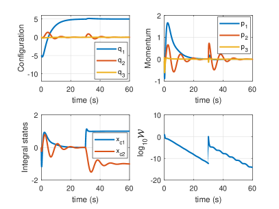
Figure 1: Simulation of the VTOL aircraft in closed-loop with an energy shaping plus integral action controller.

VIII Conclusion

In this paper, a method for designing IAC for pH system subject to matched and unmatched disturbances is presented. The proposed design extends our previous work by relaxing the restrictive assumptions of a strongly convex and separable Hamiltonian function for the open-loop system. By relaxing these assumptions, the proposed IAC is shown to be applicable to a more general class of mechanical systems that strictly contains the class considered in previous works. The method is illustrated on three examples: a PMSM with unknown load torque and mechanical friction, 2-DOF manipulator with unknown damping and a VTOL aircraft.

Lemma 2

Consider the system (1) and assume there exists some $\bar{x}$ verifying Assumption 3. If there exists a suitable coordinate transformation (8), then there exists some $\hat{x}$ satisfying (LABEL:barxiacort).

Proof:

By Assumption 3, there exists some $\bar{x}$ satisfying $\nabla_{x_{a}}\bar{\mathcal{H}}=-\bar{d}_{u},\nabla_{x_{u}}\bar{\mathcal{H}}=0_{m\times 1}$. Using this point, we define $(\bar{z}_{1},\bar{z}_{2})=(\bar{x}_{1},\bar{x}_{2})$. Using this definition, the point $\hat{x}$ can be defined using the functions $\psi$ and its inverse $\mu$:

$$(\hat{x}_{a},\hat{x}_{u})=(\mu(\bar{z}_{1},\bar{z}_{2},\bar{d}_{u}),\bar{z}_{2}).$$ (79)

It must now be verified that $\hat{x}$ satisfies (LABEL:barxiacort). To see that $\hat{x}\in{\cal E}$, first notice that $\nabla_{x_{a}}\mathcal{H}|_{x_{a}=\hat{x}_{1}}=\nabla_{x_{a}}\mathcal{H}|_{x_{a}=\bar{z}_{1}}=-\bar{d}_{u}$ and $\nabla_{x_{u}}\mathcal{H}|_{x_{a}=\hat{x}_{u}}=\nabla_{x_{u}}\mathcal{H}|_{x_{a}=\bar{z}_{2}}=0_{m\times 1}$. Thus, $\hat{x}_{a}\in{\cal E}$. Now it must be shown that $\nabla_{x_{u}}{\cal H}(\psi(\hat{x}_{a},\hat{x}_{u},\bar{d}_{u}),\hat{x}_{u})$ is equal to zero. By definition, this expression is equivalent to $\nabla_{x_{u}}{\cal H}(\bar{z}_{1},\bar{z}_{2})=\nabla_{x_{u}}{\cal H}(\bar{x}_{a},\bar{x}_{u})$, which is equal to zero by Assumption 3. $\Box\Box\Box$

Joel Ferguson was born in Australia. He received his degree in mechatronic engineering from the University of Newcastle in 2013, being awarded the Dean’s medal and University medal. Since 2014, Joel has been pursuing his Ph.D. at the University of Newcastle under the supervision of Prof. R. Middleton and Dr. A. Donaire. His research interests include nonlinear control, port-Hamiltonian systems, nonholonomic systems and robotics.

Alejandro Donaire received his degree in Electronic Engineering in 2003 and his PhD in 2009, both from the National University of Rosario, Argentina. In 2009, he took a research position at the Centre for Complex Dynamic Systems and Control, The University of Newcastle, Australia. In 2011, he was awarded the Postdoctoral Research Fellowship at the University of Newcastle. In March 2015, he joined the robotic team at PRISMA Lab, University of Naples Federico II, Italy. Since 2017, he is conducting his research activities in within Queensland University of Technology (QUT), Australia. His research interests include nonlinear system analysis and passivity theory for control design of robotics, mechatronics, marine and aerospace systems.

Romeo Ortega was born in Mexico. He obtained his BSc in Electrical and Mechanical Engineering from the National University of Mexico, Master of Engineering from Polytechnical Institute of Leningrad, USSR, and the Docteur D‘Etat from the Politechnical Institute of Grenoble, France in 1974, 1978 and 1984 respectively. He then joined the National University of Mexico, where he worked until 1989. He was a Visiting Professor at the University of Illinois in 1987-88 and at McGill University in 1991-1992, and a Fellow of the Japan Society for Promotion of Science in 1990-1991. He has been a member of the French National Research Council (CNRS) since June 1992. Currently he is a Directeur de Recherche in the Laboratoire de Signaux et Systemes (CentraleSupelec) in Gif-sur-Yvette, France. His research interests are in the fields of nonlinear and adaptive control, with special emphasis on applications. Dr Ortega has published three books and more than 290 scientific papers in international journals, with an h-index of 71. He has supervised more than 30 PhD thesis. He is a Fellow Member of the IEEE since 1999 and an IFAC Fellow since 2016. He has served as chairman in several IFAC and IEEE committees and participated in various editorial boards of international journals.

Richard H. Middleton was born on 10th December 1961 in Newcastle Australia. He received his B.Sc. (1983), B.Eng. (Hons-I)(1984) and Ph.D. (1987) from the University of Newcastle, Australia. He has had visiting appointments at the University of Illinois at Urbana-Champaign, the University of Michigan and the Hamilton Institute (National University of Ireland Maynooth). In 1991 he was awarded the Australian Telecommunications and Electronics Research Board Outstanding Young Investigator award. In 1994 he was awarded the Royal Society of New South Wales Edgeworth-David Medal; he was elected to the grade of Fellow of the IEEE starting 1999, received the M.A. Sargent Award from the Electrical College of Engineers Australia in 2004, and as a Fellow of the International Federation of Automatic Control in 2013. He has served as an associate editor, associate editor at large and senior editor of the IEEE Transactions on Automatic Control, the IEEE Transactions on Control System Technology, and Automatica, as Head of Department of Electrical Engineering and Computing at the University of Newcastle; as a panel member and sub panel chair for the Australian Research Council; as Vice President - Member Activities and also as Vice President – Conference Activities of the IEEE Control Systems Society; President (2011) of the IEEE Control Systems Society; as Director of the ARC Centre for Complex Dynamic Systems and Control; a Distinguished Lecturer for the IEEE Control Systems Society, and as a research professor at the Hamilton Institute, The National University of Ireland, Maynooth. He is currently Head of School of Electrical Engineering and Computing at the University of Newcastle. He is also Editor – System and Control Theory, of Automatica. His research interests include a broad range of Control Systems Theory and Applications, including feedback performance limitations, information limited control and systems biology.

References

• [1] H. Nijmeijer and A. van der Schaft, Nonlinear Dynamical Control Systems, 1st ed., Eds.   Springer-Verlag New York, 1990.
• [2] A. van der Schaft and D. Jeltsema, “Port-Hamiltonian systems theory: An introductory overview,” Foundations and Trends in Systems and Control, vol. 1, no. 2-3, pp. 173–378, 2014.
• [3] R. Ortega and E. Garcia-Canseco, “Interconnection and damping assignment passivity-based control: A survey,” European Journal of control, vol. 10, no. 5, pp. 432–450, 2004.
• [4] V. Petrović, R. Ortega and A. M. Stanković, “Interconnection and damping assignment approach to control of PM synchronous motors,” IEEE Transactions on Control Systems Technology, vol. 9, no. 6, pp. 811–820, 2001.
• [5] C. Batlle, A. Doria, G. Espinosa and R. Ortega, “Simultaneous interconnection and damping assignment passivity-based control: The induction machine case study”, International Journal of Control, vol. 82, no. 2, pp. 241-255, 2009.
• [6] S. Bacha, I. Munteanu and A. Bratcu, Power Electronic Converters Modeling and Control: with Case Studies, Springer-Verlag, 2013.
• [7] F. Dorfler, J.K. Johnsen and F. Allgower, “An introduction to interconnection and damping assignment passivity-based control in process engineering”, Journal of Process Control, vol. 19, no. 9, pp. 1413-1426, 2009.
• [8] J. Acosta, R. Ortega and A. Astolfi, “Interconnection and damping assignment passivity-based control of mechanical systems with underactuation degree one,” IEEE Transactions on Automatic Control, vol. 50, no. 12, pp. 1936–1955, 2005.
• [9] G. Viola, R. Ortega, R. Banavar, J. A. Acosta and A. Astolfi, “Total energy shaping control of mechanical systems: Simplifying the matching equations via coordinate changes”, IEEE Transactions Automatic Control, vol. 52, no. 6, pp. 1093-1099, 2007.
• [10] K. Fujimoto, K. Sakurama and T. Sugie, “Trajectory tracking control of port-controlled Hamiltonian systems via generalized canonical transformations,” Automatica, vol. 39, no. 12, pp. 2059–2069, 2003.
• [11] A. Donaire and S. Junco, “On the addition of integral action to port-controlled Hamiltonian systems,” Automatica, vol. 45, no. 8, pp. 1910–1916, 2009.
• [12] R. Ortega and J. G. Romero, “Robust integral control of port-Hamiltonian systems: The case of non-passive outputs with unmatched disturbances,” Systems & Control Letters, vol. 61, no. 1, pp. 11–17, 2012.
• [13] J. G. Romero, A. Donaire and R. Ortega, “Robust energy shaping control of mechanical systems,” Systems & Control Letters, vol. 62, no. 9, pp. 770–780, 2013.
• [14] A. Donaire, J. G. Romero, R. Ortega, B. Siciliano and M. Crespo, “Robust IDA-PBC for underactuated mechanical systems subject to matched disturbances,” Int. Journal of Robust and Nonlinear Control, vol. 27, no. 6, pp. 1000–1016, 2016.
• [15] J. Ferguson, R. H. Middleton and A. Donaire, “Disturbance rejection via control by interconnection of port-Hamiltonian systems,” in IEEE Conference on Decision and Control.   Osaka, Japan: IEEE, 2015, pp. 507–512.
• [16] J. Ferguson, A. Donaire and R. H. Middleton, “Integral control of port-Hamiltonian systems: non-passive outputs without coordinate transformation,” IEEE Transactions on Automatic Control, preprint, 2017.
• [17] R. Ortega, A. van der Schaft, F. Castaños and A. Astolfi, “Control by interconnection and standard passivity-based control of port-Hamiltonian Systems,” IEEE Transactions on Automatic Control, Vol. 53, No. 11, pp. 2527–2542, 2008.
• [18] C. Batlle, A. Doria-Cerezo and E. Fossas, “Robust Hamiltonian passive control for higher relative degree outputs,” IOC-DT-P-2006-25, Institut d’Organització i Control de Sistemes Industrials, E-Prints UPC, Universitat Politècnica de Catalunya, 2006.
• [19] A. A. Alonso and B. Ydstie, “Stabilization of distributed systems using irreversible thermodynamics,” Automatica, vol. 37, pp. 1739–1755, 2001.
• [20] B. Jayawardhana, R. Ortega and E. García-Canseco, “Passivity of nonlinear incremental systems: Application to PI stabilization of nonlinear RLC circuits,” Systems & Control Letters, vol. 56, no. 9-10, pp. 618–622, 2007.
• [21] A. van der Schaft, ${\cal L}_{2}$-Gain and Passivity Techniques in Nonlinear Control, 3rd ed.   Springer, 2017.
• [22] K. Fujimoto and T. Sugie, “Canonical transformation and stabilization of generalized Hamiltonian systems,” Systems & Control Letters, vol. 42, no. 3, pp. 217–227, 2001.
• [23] A. Venkatraman, R. Ortega, I. Sarras and A. van der Schaft, “Speed observation and position feedback stabilization of partially linearizable mechanical systems,” IEEE Transactions on Automatic Control, vol. 55, no. 5, pp. 1059–1074, 2010.
• [24] V. Duindam and S. Stramigioli, “Singularity-free dynamic equations of open-chain mechanisms with general holonomic and nonholonomic joints,” IEEE Transactions on Robotics, vol. 24, no. 3, pp. 517–526, 208.
• [25] D. A. Dirksz and J. M. A. Scherpen, “Power-Based setpoint control : experimental results on a planar manipulator,” IEEE Transactions on Control Systems Technology, vol. 20, no. 5, pp. 1384 – 1391, 2012.
• [26] F. Gómez-Estern and A. van der Schaft, “Physical damping in IDA-PBC controlled underactuated mechanical systems,” European Journal of Control, vol. 10, no. 5, pp. 451–468, 2004.
• [27] J. M. Lee, Introduction to Smooth Manifolds, 2nd ed., S. Axler and K. Ribet, Eds.   Springer-Verlag New York, 2012, vol. 218.