Solitons in $\mathcal{PT}$-symmetric ladders of optical waveguides

Abstract

We consider a $\mathcal{PT}$-symmetric ladder-shaped optical array consisting of a chain of waveguides with gain coupled to a parallel chain of waveguides with loss. All waveguides have the focusing Kerr nonlinearity. The array supports two co-existing solitons, an in-phase and an antiphase one, and each of these can be centred either on a lattice site or midway between two neighbouring sites. We show that both bond-centred (i.e. intersite) solitons are unstable regardless of their amplitudes and parameters of the chain. The site-centred in-phase soliton is stable when its amplitude lies below a threshold that depends on the coupling and gain-loss coefficient. The threshold is lowest when the gain-to-gain and loss-to-loss coupling constant in each chain is close to the interchain gain-to-loss coupling coefficient. The antiphase soliton in the strongly-coupled chain or in a chain close to the $\mathcal{PT}$-symmetry breaking point, is stable when its amplitude lies above a critical value and unstable otherwise. The instability growth rate of solitons with small amplitude is exponentially small in this parameter regime; hence the small-amplitude solitons, though unstable, have exponentially long lifetimes. On the other hand, the antiphase soliton in the weakly or moderately coupled chain and away from the $\mathcal{PT}$-symmetry breaking point, is unstable when its amplitude falls in one or two finite bands. All amplitudes outside those bands are stable.

I Introduction

In soliton-bearing optical systems, weak dissipative losses are typically compensated by the application of a resonant pump. The damping and driving terms break the scaling-, phase- and Galilean invariances of the underlying nonlinear Schrödinger equation. As a result, the amplitude, phase, and velocity of the damped-driven solitons are found to be fixed by the driver’s strength and dissipation coefficient DD .

Dissipative solitons in systems with competing linear and nonlinear gain and loss — systems modelled by the Ginsburg-Landau equations — are equally inflexible. The balance of nonlinearity and diffraction or dispersion singles out a one-parameter family of solitons, while the competition of gain and loss fixes a particular member of the family CGL . This inflexibility can be a disadvantage in applications where one would like the parameters of the soliton to be determined just by the initial conditions.

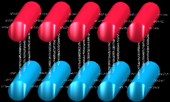
Figure 1: A $\mathcal{PT}$-symmetric ladder of coupled optical waveguides with gain (red) and loss (blue). Each guide is coupled to its left and right nearest neighbours in the horizontal plane. We are occasionally referring to this coupling as “horizontal” in the text. In addition, each guide with gain is coupled to its nearest guide with loss — this will be referred to as the “vertical coupling”.

Yet there are ways of supplying energy in a soliton-bearing system with loss, free from the above drawback. The pertinent class of approaches exploits the concept of the parity-time ($\mathcal{PT}$-) symmetry, originally developed in the context of quantum mechanics Bender . One $\mathcal{PT}$-symmetric recipe consists in the manufacturing of two identical replicas of the same system and arranging for the energy supply in one copy and energy drain in the other one. With a judicious choice of coupling, the combined system with gain and loss will contain, as its scalar reduction, the unperturbed nonlinear Schrödinger equation. As a result, this $\mathcal{PT}$-symmetric system will support families of solitons with continuously variable amplitudes, phases, and velocities.

In fact the parametric flexibility is but one of the whole range of unusual properties of optical $\mathcal{PT}$-symmetric structures. Other behaviours afforded by the symmetric application of gain and loss and unattainable with standard arrangements, include the unconventional beam refraction Musslimani ; Zheng ; Regensburger , Bragg scattering Berry_Longhi , nonreciprocal light propagation Nonreciprocal_propagation ; WGM ; Shramkova and Bloch oscillations Longhi , loss-induced transparency Guo , single-mode lasing single-mode_laser , coherent perfect absorption of light Chong , loss-induced onset of lasing loss_lase and conical diffraction Ramezani . The $\mathcal{PT}$-symmetric systems are expected to promote an efficient control of light, including all-optical low-threshold RKEC ; SXK ; Lin and asymmetric EPswitch switching and unidirectional invisibility RKEC ; Feng ; Regensburger ; Sanchez . There is also a rapidly growing interest in the context of plasmonics plasmonics , quantum optics of atomic gases Lambda , optomechanical systems OM ; Kepesides and metamaterials Lazarides ; Shramkova .

The early experimental realisations of the optical $\mathcal{PT}$ symmetry were in a directional coupler consisting of two waveguides with gain and loss Guo ; Rueter ; Kottos and in a pair of coupled whispering-gallery mode resonators WGM . The work that followed focussed on chains of $\mathcal{PT}$-symmetric couplers Regensburger ; Regensburger2 ; Miri1 ; Christo_2016 . The corresponding theoretical studies progressed from a single Schrödinger dimer RKEC ; SXK ; Miri2 ; standimer and oligomer oligomer ; Liam ; Turitsyn ; Izrailev ; Kepesides , to $\mathcal{PT}$-symmetric dimer arrays binary ; SMDK ; KPZ ; staggered ; Chernyavsky ; Miri3 . The subsequent analyses included the effects of diffraction of spatial beams and dispersion of temporal pulses, that is, included an additional spatial or temporal dimension SMDK ; Driben1 ; Driben2 ; ABSK ; BSSDK ; Driben3 . $\mathcal{PT}$-symmetric necklaces of dispersive waveguides (dispersive $\mathcal{PT}$-oligomers) were examined in Liam . For comprehensive reviews, see reviews .

In this paper, we consider an infinite chain of $\mathcal{PT}$-symmetric dimers coupled to their nearest neighbours. The coupling of the neighboring dimers is arranged in such a way that, apart from its “internal” counterpart with gain, each waveguide with loss interacts only with its two lossy neighbours (Fig 1). Likewise, each waveguide with gain is coupled only to its two neighbours with gain — besides its counterpart with loss with who they make up the $\mathcal{PT}$-symmetric entity SMDK :

$$i{\dot{u}_{n}}+{\mathfrak{C}}\Delta u_{n}+2|u_{n}|^{2}u_{n}+v_{n} =i\gamma u_{n},$$

$$i{\dot{v}_{n}}+{\mathfrak{C}}\Delta v_{n}+2|v_{n}|^{2}v_{n}+u_{n} =-i\gamma v_{n}.$$ (1)

Here $\Delta$ is the second difference operator acting on bi-infinite sequences $...,u_{-2},u_{-1},u_{0},u_{1},u_{2},...$ according to the rule

$$\Delta u_{n}=u_{n+1}-2u_{n}+u_{n-1}\quad(n=0,\pm 1,\pm 2,....).$$

In the basis of infinite-component vectors

$${\bf u}=(...,u_{-2},u_{-1},u_{0},u_{1},u_{2},...)^{T},$$

the operator $\Delta$ is represented by a tridiagonal matrix.

The $u_{n}$ is the nondimensional complex mode amplitude in the $n$th waveguide with gain, and $v_{n}$ is the amplitude in the $n$th waveguide with loss. The overdot indicates the derivative with respect to $z$, the propagation coordinate. The sign of the cubic terms corresponds to the self-focusing Kerr nonlinearity; the coefficients in front of these terms have been set to 2 by scaling the mode amplitudes. Finally, ${\mathfrak{C}}>0$ is a dimer-to-dimer coupling constant (the “horizontal” coupling in the language of Fig 1), and $\gamma\geq 0$ is the gain-loss coefficient.

The ladder-shaped chain (1) supports four families of soliton excitations SMDK . These are distinguishable by the phase difference between $u_{n}$ and $v_{n}$, and by the centring of the soliton relative to lattice sites. In the continuum limit, their stability has been classified in Driben1 ; ABSK . Ref Susanto considered the anticontinuum limit, under an additional assumption of $\gamma\to 0$. In the present paper we study the discrete solitons in the entire range of their amplitudes, for all values of the coupling ${\mathfrak{C}}$ and all physically admissible values of $\gamma$.

We will demonstrate that the soliton stability problem can be decomposed into an eigenvalue problem for perturbations belonging to the same symmetric manifold as the stationary soliton itself, and perturbations that take the evolution out of the symmetry. This decomposition alone is sufficient to classify the stability of the bond-centred solitons — which happen to be all unstable against a perturbation in the symmetric manifold. In contrast, the instability of the site-centred solitons can only be nucleated by nonsymmetric perturbations. In the latter case, the advantage of our decomposition is that it reduces the underlying two-component eigenvalue problem to a much simpler one-component problem.

We will show that stability properties of the in-phase and antiphase site-centred soliton are completely determined just by two combinations of ${\mathfrak{C}}$, $\gamma$ and the soliton’s amplitude. The stability domain of the in-phase soliton admits a simple characterisation in terms of a single function relating these two self-similar combinations. As a result, for each ${\mathfrak{C}}$ and $\gamma$ we will be able to determine a critical value of the amplitude above which the soliton becomes unstable.

Stability properties of the antiphase soliton in a strongly-coupled chain or in a weakly or moderately coupled chain close to its $\mathcal{PT}$-symmetry breaking point, follow an opposite pattern. Here, the soliton instability sets in below a critical amplitude. Reducing the inter-dimer coupling or turning down the gain-loss coefficient of the chain, changes the topography of this soliton’s parameter space. Namely, the weakly or moderately coupled array away from the $\mathcal{PT}$-symmetry breaking threshold displays one or two bands of unstable amplitudes, with all antiphase solitons outside those bands being stable.

The outline of the paper is as follows. Section II summarises stability properties of two solitons arising in the continuum limit of the array (1). In section III, we introduce four discrete solitons: the in-phase and antiphase site-centred soliton, and the in- and out-of-phase bond-centred one. The subsequent section IV lays out the general framework of our stability analysis and draws some general conclusions.

In section V we classify the stability of the in-phase solitons while section VI focusses on the antiphase variety. Some technical results on eigenvalues playing the central role in our analysis have been relegated to eight appendices. Finally, section VII summarises conclusions of this study and contrasts them with the earlier results of SMDK and Susanto .

II Continuum limit: summary

If the characteristic wavelength in the chain is much greater than ${\mathfrak{C}}^{-1/2}$, the $\mathcal{PT}$-symmetric lattice (1) reduces to a system of two partial differential equations:

$$i{\dot{u}}+u_{xx}+2|u|^{2}u+v =i\gamma u,$$

$$i{\dot{v}}+v_{xx}+2|v|^{2}v+u =-i\gamma v.$$ (2)

This $\mathcal{PT}$-symmetric system of coupled nonlinear Schrödinger equations was considered in SMDK ; Driben1 ; ABSK ; BSSDK . Results of the previous analyses can be summarised as follows.

(1) For each $\gamma<1$, there are two continuous families of coexisting solitons. Each family is characterised by its own value of the phase difference between the $u$- and $v$-component. Representatives of the two families with equal amplitudes have unequal propagation constants SMDK .

(2) The soliton stability and internal dynamics are determined by a single self-similar combination $\eta=2\sqrt{1-\gamma^{2}}/A^{2}$ of the gain-loss coefficient $\gamma$ and the soliton’s amplitude, $A$ ABSK .

(3) The in-phase solitons with amplitudes smaller than $\mathcal{A}_{0}=\sqrt{\frac{2}{3}}(1-\gamma^{2})^{1/4}$ are stable, and with amplitudes greater than $\mathcal{A}_{0}$, unstable Driben1 ; ABSK . All antiphase solitons are unstable; however the lifetimes of the antiphase solitons with small amplitudes are exponentially long ABSK ; Dima_Deconinck2 .

In this paper, we will extend these considerations to localised solutions of the discrete system (1).

III Discrete solitons

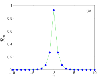
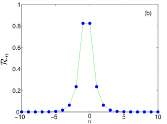
Figure 2: The two single-hump solutions of equation (7) with the same $h$. (In these plots, $h=\sqrt{2}$.) The left panel shows the form of $|u_{n}|$ and $|v_{n}|$ for the site-centred soliton (both for the in-phase and antiphase one). The right panel illustrates the magnitude profile of the bond-centred soliton — again, for the in- and out-of-phase one alike.

The dispersion relations for the small-amplitude harmonic waves in the system (1) are

$$\omega=\pm\omega_{0}-4{\mathfrak{C}}\sin^{2}\frac{k}{2},\quad\omega_{0}=\sqrt{1-\gamma^{2}}.$$

In what follows, we assume that the trivial solution, $u_{n}=v_{n}=0$, is stable: $0\leq\gamma\leq 1$.

For future convenience, we perform the change of variables

$$u_{n}=e^{i\theta}a_{n}+b_{n},\quad v_{n}=e^{i\theta}b_{n}-a_{n},$$ (3)

where $\theta=\arcsin\gamma$. This transformation diagonalises the linear part of equations (1) BSSDK ; Liam :

$$i{\dot{a}}_{n}+{\mathfrak{C}}\Delta a_{n}-\omega_{0}a_{n}+\frac{|u_{n}|^{2}u_{n}-e^{-i\theta}|v_{n}|^{2}v_{n}}{\omega_{0}}=0,$$

$$i{\dot{b}}_{n}+{\mathfrak{C}}\Delta b_{n}+\omega_{0}b_{n}+\frac{e^{-i\theta}|u_{n}|^{2}u_{n}+|v_{n}|^{2}v_{n}}{\omega_{0}}=0,$$ (4)

where $u_{n}$ and $v_{n}$ denote the linear combinations (3).

The system (1) has two invariant manifolds where the evolution is conservative ABSK . Indeed, the equations (4) admit a reduction $a_{n}=0$, $b_{n}=\phi_{n}$ to the scalar discrete nonlinear Schrödinger equation

$$i{\dot{\phi}_{n}}+{\mathfrak{C}}\Delta\phi_{n}+\omega_{0}\phi_{n}+2|\phi_{n}|^{2}\phi_{n}=0.$$ (5)

(Note that under this reduction, $u_{n}=\phi_{n}$ and $v_{n}=e^{i\theta}\phi_{n}$.) A different, independent, scalar reduction arises by letting $b_{n}=0$, $a_{n}=\phi_{n}$. The equations (4) become

$$i{\dot{\phi}_{n}}+{\mathfrak{C}}\Delta\phi_{n}-\omega_{0}\phi_{n}+2|\phi_{n}|^{2}\phi_{n}=0.$$ (6)

(This time, $u_{n}=e^{i\theta}\phi_{n}$ and $v_{n}=-\phi_{n}$.)

In this paper, we are focussing on localised solutions of (5) and (6): $|\mathcal{\phi}_{n}|\to 0$ as $|n|\to\infty$. The simplest solutions of this sort are separable; these are given by

$$\phi_{n}=e^{i\beta z}A\mathcal{R}_{n}.$$

Here $A>0$ is an arbitrary amplitude and $\mathcal{R}_{n}$ solves

$$\frac{1}{h^{2}}\Delta\mathcal{R}_{n}-\mathcal{R}_{n}+2{\mathcal{R}}_{n}^{3}=0,$$ (7)

where $h$ is the amplitude-to-coupling ratio:

$$h=\frac{A}{\sqrt{\mathfrak{C}}}.$$ (8)

In what follows, we are referring to the corresponding solutions of (4) as solitons.

Equation (7) determines the profile of the localised solution and $h$ has the meaning of discretisation stepsize in this equation. In the case of the reduction (5), the propagation constant $\beta$ is given by

$$\beta=A^{2}+\omega_{0},$$ (9)

while the equation (6) requires

$$\beta=A^{2}-\omega_{0}.$$ (10)

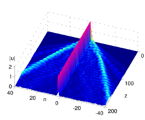
Figure 3: The formation of a soliton out of a gaussian initial condition $u_{n}(0)=e^{i(\theta+\chi)}A_{\rm gs}e^{-n^{2}}$, $v_{n}(0)=-A_{\rm gs}e^{-n^{2}}$. Here $\chi$ is a phase mismatch taking the initial condition out of the scalar reduction (6). In this plot the parameters of the lattice are ${\mathfrak{C}}=0.3$ and $\gamma=0.93$; the amplitude of the gaussian $A_{\rm gs}=2$ and the mismatch $\chi=0.3$. Note small-amplitude oscillations of the soliton’s amplitude — the non-oscillatory soliton would result from the gaussian with $\chi=0$.

We note that equations (5)-(6) admit no localised separable solutions with complex $\mathcal{R}_{n}$ (except for the trivial situation where all $\mathcal{R}_{n}$ share the same, $n$-independent, phase factor) HT . Therefore, equation (7) is the most general equation for localised profiles.

Each localised solution of (7) gives rise to two families of separable solutions of the original system (1), with ${\mathfrak{C}}=(A/h)^{2}$. The first family corresponds to the $a_{n}=0$ reduction of Eq.(4). When the gain-loss coefficient $\gamma\to 0$, the $u_{n}$ and $v_{n}$ components of any solution in this family become equal: $v_{n}\to u_{n}$. In contrast, the components of any separable solution corresponding to the $b_{n}=0$ reduction become equal in magnitude but opposite in sign: $v_{n}\to-u_{n}$. Because of this simple and noticeable difference, the localised separable solutions with $a_{n}=0$ will be called the in-phase solitons, and those with $b_{n}=0$ the antiphase ones. (By continuity, we will use this terminology even in the $\gamma\to 1$ limit where the difference between the two families becomes negligible.)

Note that the soliton solution of Eq.(4) with $a_{n}=0$ and amplitude $A$, has a larger propagation constant than the $(b_{n}=0)$-soliton of the same amplitude. For this reason, the in-phase separable solution was referred to as the high-frequency soliton in ABSK , and the one with $b_{n}=0$ as the low-frequency one.

Equation (7) has a variety of localised solutions, in particular two fundamental, i.e., single-hump, nonlinear modes. One of these is centred on the site with $n=0$ (the so-called Sievers-Takeno mode) and the other one midway between the sites with $n=0$ and $n=1$ (the Page mode) KC ; LST ; KK ; PKF ; Herrmann . We will be referring to the former as the ‘site-centred’ mode, and the latter as ‘bond-centred’. Both solutions exist for all $0<h<\infty$ ABK ; both satisfy $\mathcal{R}_{n}>0$ for all $n$ Herrmann . We depict these solutions in Fig. 2.

Thus there are four fundamental solitons in the dimer array (1): the in-phase and antiphase site-centred soliton, and the in-phase and antiphase bond-centred one. The distribution of the waveguide mode magnitudes in the site- and bond-centred soliton is shown in Fig 2. The phases of $u_{n}$ and $v_{n}$ remain constant as $n$ grows or decreases; hence there is no flow of energy along the array. On the other hand, the phase difference between $u_{n}$ and $v_{n}$ reflects a nonzero energy flux from the gaining to the losing waveguide of each dimer.

Small $h$ correspond to the continuum limit (small soliton amplitudes or strongly coupled sites). As $h\to 0$, the site-centred and bond-centred solutions satisfy $\mathcal{R}_{n}\to\,\mathrm{sech}(hn)$ and $\mathcal{R}_{n}\to\,\mathrm{sech}[h(n-~{}\frac{1}{2})]$, respectively. Large $h$ pertain to the anti-continuum limit (large amplitudes or weak dimer-to dimer coupling).

Before proceeding to stability analysis, we note that discrete solitons and their breather-like perturbations emerge from a broad class of initial conditions. Fig 3 shows the formation of a soliton from a gaussian with generic amplitude and phase.

IV Stability framework

IV.1 The in-phase soliton

Consider the in-phase soliton first. Letting

$$a_{n}=e^{i\beta z}\left[\mathrm{Re}(p^{(1)}_{n}e^{\mu z})+i\,\mathrm{Re}(p_{n}^{(2)}e^{\mu z})\right],$$

$$b_{n}=e^{i\beta z}\left[A\mathcal{R}_{n}+\mathrm{Re}(q^{(1)}_{n}e^{\mu z})+i\,\mathrm{Re}(q_{n}^{(2)}e^{\mu z})\right],$$

where $\mathcal{R}_{n}$ is a solution of (7), $\beta$ is as in (9), and $p_{n}^{(1,2)}$, $q_{n}^{(1,2)}$, and $\mu$ are complex, we linearise equations (4) in $p_{n}^{(1,2)}$ and $q_{n}^{(1,2)}$. This gives an eigenvalue problem

$$\mathcal{L}{\vec{p}}_{n}+\omega_{0}{\vec{p}}_{n}=\mu J{\vec{p}}_{n},$$ (11a)

$$\mathcal{L}{\vec{q}}_{n}-\omega_{0}{\vec{q}}_{n}+4\gamma A^{2}\mathcal{R}_{n}^{2}\sigma_{1}{\vec{p}}_{n}=\mu J{\vec{q}}_{n},$$ (11b)

where the operator

$$\mathcal{L}=\left(\begin{array}[]{cc}-{\mathfrak{C}}\Delta+\beta-6A^{2}\mathcal{R}_{n}^{2}&0\\ 0&-{\mathfrak{C}}\Delta+\beta-2A^{2}\mathcal{R}_{n}^{2}\end{array}\right)$$

acts on two-component complex sequences

$${\vec{p}}_{n}=\left(\begin{array}[]{c}p_{n}^{(1)}\\ p_{n}^{(2)}\end{array}\right),\quad{\vec{q}}_{n}=\left(\begin{array}[]{c}q_{n}^{(1)}\\ q_{n}^{(2)}\end{array}\right).$$

The $J$ in the right-hand sides of (11a)-(11b) denotes a unimodular skew-symmetric matrix:

$$J=\left(\begin{array}[]{lr}0&-1\\ 1&0\end{array}\right),$$

and $\sigma_{1}$ in (11b) is the conventional Pauli matrix.

The purpose of the stability analysis is to determine whether the eigenvalue problem (11) has eigenvalues $\mu$ with nonzero real part. If it has, the soliton is unstable; if it has not, the soliton is classified as linearly stable.

The continuous spectrum of $\mu$’s occupies two opposite pairs of bands on the imaginary axis: $\mu=\pm i\omega_{1,2}$, where

$$\beta+\omega_{0}\leq\omega_{1}\leq\beta+\omega_{0}+4{\mathfrak{C}},$$ (12)

$$\beta-\omega_{0}\leq\omega_{2}\leq\beta-\omega_{0}+4{\mathfrak{C}}.$$ (13)

Outside the domain of intersection of the bands (12) and (13), the problem (11) may have discrete eigenvalues.

To find the discrete eigenvalues, one does not have to solve the full system (11). Indeed, one class of eigenvectors is selected simply by letting ${\vec{p}}_{n}=0$; this choice selects perturbations belonging to the scalar Schrödinger equation (5). The associated ${\vec{q}}_{n}$ satisfies

$$\mathcal{L}{\vec{q}}_{n}-\omega_{0}{\vec{q}}_{n}=\mu J{\vec{q}}_{n},$$ (14)

the linearised eigenvalue problem for the scalar discrete nonlinear Schrödinger equation.

It is well known that for the bond-centred soliton, the operator $J^{-1}(\mathcal{L}-\omega_{0}I)$ in (14) has positive eigenvalues LST ; KK ; PKF — and so the bond-centred soliton of the scalar nonlinear Schrödinger equation (5) is unstable. This observation implies that the bond-centred in-phase soliton of the vector equation (1) is unstable for all ${\mathfrak{C}}$, $\gamma$, and $A$.

On the other hand, the site-centred soliton of the scalar Schrödinger equation (5) is stable for all $A$ and ${\mathfrak{C}}$ LST ; KK ; PKF . The operator $J^{-1}(\mathcal{L}-\omega_{0}I)$ in this case has only pure imaginary eigenvalues: two zeros, two pairs of opposite nonzero imaginary eigenvalues and two bands of continuous spectrum on the imaginary axis:

$$\mu=\pm i\omega_{2},\quad A^{2}\leq\omega_{2}\leq A^{2}+4{\mathfrak{C}}.$$ (15)

This does not yet guarantee that the corresponding soliton of the vector equations (1) is stable; the stability of the latter will be determined by eigenvectors of (11) with ${\vec{p}}_{n}\neq 0$. These correspond to linear evolutions that do not satisfy the scalar reduction (5).

The nontrivial sequences ${\vec{p}}_{n}\neq 0$ can be found as eigenvectors of the eigenvalue problem (11a). This is a significant simplification as the dimension of the matrix $\mathcal{L}+\omega_{0}I$ in (11a) is half the dimension of the full triangular matrix

$$\left(\begin{array}[]{cc}\mathcal{L}+\omega_{0}I&0\\ 4\gamma A^{2}\mathcal{R}_{n}^{2}\sigma_{1}&\mathcal{L}-\omega_{0}I\end{array}\right)$$

in (11). Once the ${\vec{p}}_{n}$ and the associated eigenvalue $\mu$ have been found, Eq.(11b) becomes a nonhomogeneous equation with the right-hand side determined by ${\vec{p}}_{n}$:

$$\mathfrak{N}{\vec{q}}_{n}=-4\gamma A^{2}\mathcal{R}_{n}^{2}\sigma_{1}{\vec{p}}_{n}.$$ (16)

Here $\mathfrak{N}$ is a nonhermitian operator defined by

$$\mathfrak{N}=\mathcal{L}-\omega_{0}I-\mu J.$$

The two-component eigenvector

$$\left(\begin{array}[]{c}{\vec{p}}_{n}\\ {\vec{q}}_{n}\end{array}\right)$$ (17)

of the full “triangular” eigenvalue problem (11) exists if the equation (16) has a solution with

$$\sum_{n=-\infty}^{\infty}\left(|q_{n}^{(1)}|^{2}+|q_{n}^{(2)}|^{2}\right)<\infty.$$

Whether the finite-norm solution ${\vec{q}_{n}}$ exists or not, depends on whether the kernel space of the adjoint operator

$$\mathfrak{N}^{\dagger}=\mathcal{L}-\omega_{0}I+\mu^{*}J$$

is empty, and if not — whether the right-hand side in (16) is orthogonal to the kernel. For the given eigenvalue $\mu$ in (11a), the operator $\mathfrak{N}^{\dagger}$ has a nonempty kernel space only if there is a sequence ${\vec{y}_{n}}$ such that

$$(\mathcal{L}-\omega_{0}I){\vec{y}_{n}}=-\mu^{*}J{\vec{y}_{n}},$$

that is, if $-\mu^{*}$ coincides with one of the (pure imaginary) eigenvalues of the symplectic operator $J^{-1}(\mathcal{L}-\omega_{0}I)$, or falls in its continuous spectrum occupying two bands in (15). Therefore if $\mu$ has a nonzero real part — the situation that concerns us here — the kernel space of $\mathfrak{N}^{\dagger}$ is empty and the two-component eigenvector (17) does exist.

Thus the stability analysis of the in-phase soliton reduces to the solution of the eigenvalue problem (11a). All unstable eigenvalues of (11a) (if exist) are automatically eigenvalues of the full eigenvalue problem (11).

IV.2 The antiphase soliton

In the case of the antiphase soliton, we let

$$a_{n}=e^{i\beta z}\left[A\mathcal{R}_{n}+\mathrm{Re}(p^{(1)}_{n}e^{\mu z})+i\,\mathrm{Re}(p_{n}^{(2)}e^{\mu z})\right],$$

$$b_{n}=e^{i\beta z}\left[\mathrm{Re}(q^{(1)}_{n}e^{\mu z})+i\,\mathrm{Re}(q_{n}^{(2)}e^{\mu z})\right],$$

where, as before, $\mathcal{R}_{n}$ is a solution of (7) and $p_{n}^{(1,2)}$, $q_{n}^{(1,2)}$, $\mu$ are complex. This time, however, $\beta$ is given by (10) rather than (9). Linearising equations (4) in $p_{n}^{(1,2)}$ and $q_{n}^{(1,2)}$ gives

$$\mathcal{L}{\vec{q}}_{n}-\omega_{0}{\vec{q}}_{n}=\mu J{\vec{q}}_{n},$$ (18a)

$$\mathcal{L}{\vec{p}}_{n}+\omega_{0}{\vec{p}}_{n}-4\gamma A^{2}\mathcal{R}_{n}^{2}\sigma_{1}{\vec{q}}_{n}=\mu J{\vec{p}}_{n}.$$ (18b)

The analysis of the eigenvalue problem (18) is similar to the analysis for the problem (11). Letting ${\vec{q}}_{n}=0$ gives the linearised eigenvalue problem for the scalar nonlinear Schrödinger equation (6):

$$(\mathcal{L}+\omega_{0}I){\vec{p}}_{n}=\mu J{\vec{p}}_{n}.$$ (19)

There are positive eigenvalues in the case of the bond-centred soliton of the scalar equation (6); this implies instability of the bond-centred antiphase soliton of the vector equation (1).

In the case of the site-centred soliton, the spectrum of (19) consists of two zeros, two pairs of opposite nonzero imaginary eigenvalues and two bands of continuous spectrum on the imaginary axis: $\mu=\pm i\omega_{1}$, where

$$A^{2}\leq\omega_{1}\leq A^{2}+4{\mathfrak{C}}.$$

Therefore, in order to detect instabilities of the site-centred soliton one has to turn to eigenvectors with ${\vec{q}}_{n}\neq 0$.

The eigenvalues pertaining to ${\vec{q}}_{n}\neq 0$ are determined by solving the “reduced” eigenvalue problem (18a). The ${\vec{p}}_{n}$-component of the eigenvector $({\vec{p}}_{n},{\vec{q}}_{n})$ is then recovered from the solution of the nonhomogeneous equation (18b). The question that concerns us here is whether there are any eigenvalues with nonzero real part; for those $\mu$, the nonhomogeneous equation (18b) has a finite-norm solution (see the argument in the previous subsection). Therefore the full triangular matrix in (18) has an unstable eigenvalue as long as the half-size matrix in (18a) has one.

IV.3 Symplectic eigenvalue problem

Since the general instability of the in- and out-of-phase bond-centred solitons has been established, we only need to consider the site-centred ones in what follows.

Starting with the in-phase soliton and forming (infinite-component) vectors ${\bf p}^{(1)}$ and ${\bf p}^{(2)}$ out of the elements of the sequences $p_{n}^{(1)}$ and $p_{n}^{(2)}$, respectively, we rename ${\bf p}^{(1)}={\bf g}$ and ${\bf p}^{(2)}={\bf f}$ for notational convenience. The eigenvalue problem (11a) is then written in the matrix form:

$$\left(\begin{array}[]{cc}L_{+}+\sigma I&0\\ 0&L_{-}+\sigma I\end{array}\right)\left(\begin{array}[]{c}{\bf g}\\ {\bf f}\end{array}\right)=\lambda J\left(\begin{array}[]{c}{\bf g}\\ {\bf f}\end{array}\right).$$ (20)

Here $L_{+}$ and $L_{-}$ are symmetric matrices with elements

$$(L_{+})_{mn}=-\Delta_{mn}+h^{2}(1-6\mathcal{R}^{2}_{n})\delta_{mn},$$ (21)

$$(L_{-})_{mn}=-\Delta_{mn}+h^{2}(1-2\mathcal{R}^{2}_{n})\delta_{mn},$$ (22)

where

$$\Delta_{mn}=\delta_{m,n+1}+\delta_{m,n-1}-2\delta_{mn},$$

$h$ is as in (8), and $\mathcal{R}_{n}$ is the site-centred single-hump solution of Eq. (7) (the Sievers-Takeno mode). In (20), we have denoted $\lambda=\mu/{\mathfrak{C}}$ and introduced a parameter $\sigma=2\omega_{0}/{\mathfrak{C}}>0$.

Turning to the antiphase soliton and treating the sequences $q_{n}^{(1)}$ and $q_{n}^{(2)}$ as infinite-component vectors ${\bf g}$ and ${\bf f}$, respectively, the eigenvalue problem (18a) is represented in the same form (20) — but with $\sigma=-2\omega_{0}/{\mathfrak{C}}<0$.

Therefore, equation (20) with $\sigma$ varying from negative to positive values defines the stability problem both for the in- and the out-of-phase soliton. Here

$$\sigma=\left\{\begin{array}[]{lr}\phantom{-}2\omega_{0}/{\mathfrak{C}},&\mbox{in-phase \ soliton};\\ -2\omega_{0}/{\mathfrak{C}},&\mbox{antiphase \ soliton}.\end{array}\right.$$ (23)

Note that the single-hump site-centred solution ${\mathcal{R}}_{n}$ is uniquely specified by the value of the parameter $h$. This means that the stability properties of the soliton with amplitude $A$, in the system (1) with coupling ${\mathfrak{C}}$ and gain-loss coefficient $\gamma$, are completely determined by two combinations of those three parameters: $\sigma$ and $h$.

The combination $\sigma$ in (23) is a structural parameter. It is fixed by the coupling constant ${\mathfrak{C}}$ and the gain/loss coefficient $\gamma$ — but does not depend on the soliton’s amplitude. On the other hand, $h$ in (8) is the amplitude of a particular solution under scrutiny normalised by the coupling: $h=A/\sqrt{{\mathfrak{C}}}$. Solitons with different amplitudes and in systems with different couplings and gain-loss coefficients have the same stability properties as long as they share the values of $\sigma$ and $h$.

It is fitting to note that a self-similarity of this sort was previously encountered in the continuum limit of the system (1). There, the stability of solitons was determined by a single similarity parameter $\eta=2\sqrt{1-\gamma^{2}}/A^{2}$ ABSK .

According to Eq.(7), the matrix $L_{-}$ has a zero eigenvalue, with the eigenvector $\mathcal{R}_{n}$. Keeping in mind that $\mathcal{R}_{n}>0$ for all $n$, equation (7) can be cast in the form

$$h^{2}(1-2{\mathcal{R}}_{n}^{2})=\frac{\Delta\mathcal{R}_{n}}{\mathcal{R}_{n}}.$$ (24)

Making use of the identity (24), the quadratic form $\langle{\bf y}|L_{-}|{\bf y}\rangle$ with an arbitrary ${\bf y}=\{y_{n}\}$ admits the following representation:

$$\sum_{nm}y_{n}(L_{-})_{nm}y_{m}=\sum_{n}\frac{(y_{n}\mathcal{R}_{n+1}-\mathcal{R}_{n}y_{n+1})^{2}}{\mathcal{R}_{n}\mathcal{R}_{n+1}}.$$

This representation implies that the matrix $L_{-}$ does not have any negative eigenvalues.

On the other hand, one can readily check that the matrix $L_{+}$ has a negative eigenvalue. A simple upper bound for it is given by equation (61) in Appendix A. The negative eigenvalue is single.

In fact, the operators (21) and (22) are not unfamiliar in the soliton stability literature. These infinite-dimensional matrices occurred in the studies of the scalar discrete nonlinear Schrödinger equation — where some of their properties were established. In particular, it was shown that the operator $L_{+}$ corresponding to the site-centred soliton has a single negative eigenvalue LST ; KK . (Had there been two negative eigenvalues, the site-centred scalar soliton would have been unstable. In actual fact, stability is a firmly established property of that solution LST ; KK ; PKF .)

The operator

$$J^{-1}\left(\begin{array}[]{cc}L_{+}+{\sigma}I&0\\ 0&L_{-}+{\sigma}I\end{array}\right)$$ (25)

in (20), is symplectic, that is, generates a hamiltonian flow. The spectrum of symplectic operators consists of pairs of pure-imaginary values, real pairs, and complex quadruplets. If $\lambda$ is a real or pure imaginary point of spectrum, then $-\lambda$ is another one; if a complex $\lambda$ is in the spectrum, then so are $\lambda^{*}$, $-\lambda$, and $-\lambda^{*}$ Arnold .

The continuous spectrum of $\lambda$ lies on the imaginary axis and consists of two bands: $\lambda=\pm i\omega$, where $\sigma+h^{2}\leq\omega\leq\sigma+4+h^{2}$. When $\sigma>0$ (the in-phase soliton), the bands are separated by a gap, whereas when $\sigma<0$ (the antiphase soliton), the bands overlap. See Fig 4.

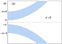
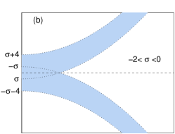
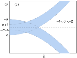
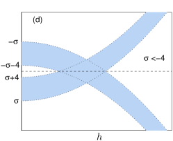
Figure 4: Two bands of continuous spectrum of the operator (25) on the $(h,\omega)$-plane, in four different intervals of $\sigma$.

When $\sigma=0$, equation (20) coincides with the eigenvalue problem for the scalar nonlinear Schrödinger equation, with no dissipative or driving terms. It is important to keep in mind, however, that the problem (20) with ${\sigma}=0$ does not result from the coupled waveguides with $\gamma=0$. The value ${\sigma}=0$ corresponds to $\gamma=1$ rather than $\gamma=0$. The significance of this value is that as $\gamma$ is increased through 1, the in-phase and antiphase solitons merge and disappear. As for the “no-gain, no-loss” ($\gamma=0$) pair of waveguides, it is represented by a nonzero $\sigma$ (${\sigma}=\pm 2/{\mathfrak{C}}$) and is not special as far as the eigenvalue problem (20) is concerned.

The scalar discrete nonlinear Schrödinger equation has two zero eigenvalues in its linearised spectrum, stemming from its U(1) phase invariance and the transformation to the linearly growing phase. Accordingly, the eigenvalue problem (20) with $\sigma=0$ has two zero eigenvalues. As ${\sigma}$ deviates from zero, the two eigenvalues move out of the origin.

Finally we note that the eigenvalue problem (20) with general $\sigma$ occurred previously in a context unrelated to the $\mathcal{PT}$-symmetry. (Specifically, it appeared in the analysis of the transverse stability of the one-dimensional soliton in the scalar two-dimensional lattice PY .) The authors of PY have established some useful properties of eigenvalues in the anticontinuum limit $h\to\infty$. We make contact with those results in what follows.

V In-phase soliton

V.1 Stability domain

In this and the next section the word “soliton” refers to the site-centred soliton (the Sievers-Takeno mode).

In the case of the in-phase soliton ($\sigma>0$), the eigenvalue problem (20) is amenable to simple analysis. The smallest eigenvalue of the operator $L_{-}+\sigma I$ equals ${\sigma}$; therefore, the matrix $L_{-}+{\sigma}I$ is positive definite and admits an inverse. Hence the problem (20) can be written as a generalised eigenvalue problem for the vector $\bf g$:

$$(L_{+}+{\sigma I}){\bf g}=-\lambda^{2}(L_{-}+{\sigma I})^{-1}{\bf g}.$$ (26)

The operator on the left in (26) is symmetric, and the one on the right is symmetric and positive definite. The lowest eigenvalue $-\lambda^{2}$ is given by the minimum of the Rayleigh quotient

$$-\lambda^{2}=\min\frac{\langle{\bf g}|L_{+}+{\sigma I}|{\bf g}\rangle}{\langle{\bf g}|(L_{-}+{\sigma I})^{-1}|{\bf g}\rangle}.$$ (27)

Let $E_{0}=E_{0}(h)$ denote the (single) negative eigenvalue of $L_{+}$. The minimum in (27) is nonnegative (hence the soliton is stable) if the smallest eigenvalue of the operator in the numerator is nonnegative: $E_{0}(h)+\sigma\geq 0$.

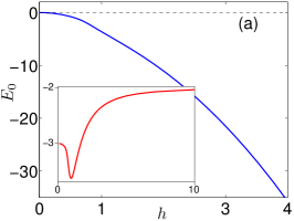
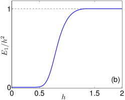
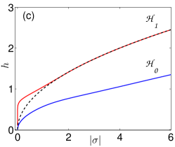
Figure 5: The negative (a) and positive (b) eigenvalue of the matrix $L_{+}$ computed numerically. In (b), the eigenvalue $E_{1}$ is shown relative to $h^{2}$ (the lower endpoint of the continuous spectrum). In a similar way, the inset in (a) gives $E_{0}/h^{2}$. Panel (c) displays the functions $\mathcal{H}_{1}(|\sigma|)$ (the inverse of $E_{1}(h)$) and $\mathcal{H}_{0}(|\sigma|)$ (inverse of $-E_{0}(h)$). The dashed line here is $h=|\sigma|^{1/2}$.

The eigenvalue $E_{0}$, calculated numerically for a sequence of $h$ values, is plotted in Fig 5 (a). It is clear from the figure that the function $\sigma=-E_{0}(h)$ grows, monotonically, from zero to infinity as $h$ varies over the positive part of the axis. Denoting $h=\mathcal{H}_{0}(\sigma)$ its inverse function, the stability condition for the in-phase soliton can be written as

$$h\leq\mathcal{H}_{0}(\sigma).$$ (28)

The function $\mathcal{H}_{0}(\sigma)$, determined numerically, is plotted in Fig.5(c). Equation (61) of the Appendix A provides a simple upper bound for this function:

$$\mathcal{H}_{0}(\sigma)<\sqrt{\sigma/2},\quad 0<\sigma<\infty.$$ (29)

Using equations (70) and (77) in the corresponding Appendices, we obtain its small- and large-$\sigma$ asymptotic behaviours:

$$\mathcal{H}_{0}(\sigma)=\sqrt{\frac{\sigma}{3}}\left[1-\frac{\sigma}{90}+\frac{7}{16200}\sigma^{2}+O(\sigma^{3})\right],\quad\sigma\to 0;$$ (30)

$$\mathcal{H}_{0}(\sigma)=\sqrt{\frac{\sigma}{2}}\left[1-\frac{2}{\sigma}+\frac{10}{3}\frac{1}{\sigma^{2}}+O\left(\frac{1}{\sigma^{3}}\right)\right],\quad\sigma\to\infty.$$ (31)

The stability domain admits a clear characterisation in terms of the soliton’s amplitude and the original parameters of the model (1). Recalling that $h=A/\sqrt{{\mathfrak{C}}}$ and $\sigma=2\sqrt{1-\gamma^{2}}/{\mathfrak{C}}$, we infer from (28) that the in-phase soliton is stable if its amplitude satisfies

$$A\leq{\mathcal{A}}_{0}(\gamma,{\mathfrak{C}}),$$ (32)

and unstable otherwise. Here $\mathcal{A}_{0}$ is a function of the coupling and gain-loss coefficient:

$$\mathcal{A}_{0}(\gamma,{\mathfrak{C}})=\sqrt{{\mathfrak{C}}}\,\mathcal{H}_{0}\!\left(\frac{2\sqrt{1-\gamma^{2}}}{{\mathfrak{C}}}\right),$$ (33)

with $h=\mathcal{H}_{0}(\sigma)$ being the inverse of the function $\sigma=-E_{0}(h)$. For each fixed value of ${\mathfrak{C}}$ we will be referring to the function $\mathcal{A}_{0}(\gamma,{\mathfrak{C}})$ as the instability threshold.

Equation (29) translates into a simple upper bound for the threshold:

$$\mathcal{A}_{0}(\gamma,{\mathfrak{C}})\leq(1-\gamma^{2})^{1/4}.$$ (34)

More accurate estimates for the boundary of the stability domain are available in two opposite limits. In the limit $\sqrt{1-\gamma^{2}}/{\mathfrak{C}}\to 0$, the approximate expression for $\mathcal{A}_{0}$ stems from equation (30):

$$\mathcal{A}_{0}=\left(\frac{2}{3}\right)^{1/2}(1-\gamma^{2})^{1/4}\left[1-\frac{1}{45}\frac{\sqrt{1-\gamma^{2}}}{{\mathfrak{C}}}+\frac{7}{4050}\frac{1-\gamma^{2}}{{\mathfrak{C}}^{2}}+O\left(\frac{(1-\gamma^{2})^{3/2}}{{\mathfrak{C}}^{3}}\right)\right].$$ (35)

(The first term in this expression reproduces the instability threshold for the solitons in the $\mathcal{PT}$-symmetric coupler consisting of two parallel guiding planes Driben1 ; ABSK .)

In the weak coupling limit (${\mathfrak{C}}/\sqrt{1-\gamma^{2}}\to 0$), an approximate expression for the instability threshold follows from equation (31):

$$\mathcal{A}_{0}=(1-\gamma^{2})^{1/4}\left[1-\frac{{\mathfrak{C}}}{\sqrt{1-\gamma^{2}}}+\frac{5}{6}\frac{{\mathfrak{C}}^{2}}{1-\gamma^{2}}+O\left(\frac{{\mathfrak{C}}^{3}}{(1-\gamma^{2})^{3/2}}\right)\right].$$ (36)

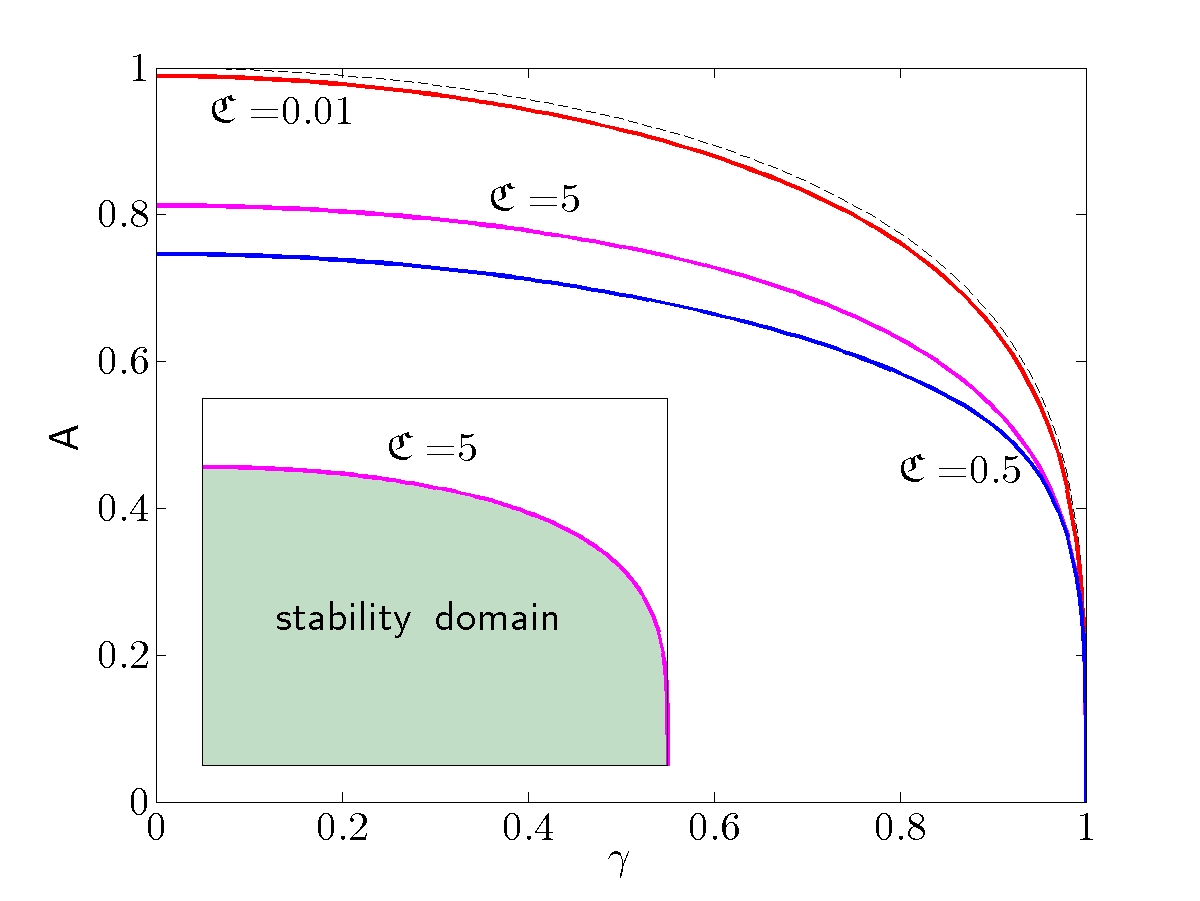
Figure 6: The in-phase soliton instability threshold for three different values of ${\mathfrak{C}}$. Solid lines, top to bottom: ${\mathfrak{C}}=0.01$, ${\mathfrak{C}}=5$, ${\mathfrak{C}}=0.5$. The dashed line demarcates the upper bound of the stability domain provided by equation (34). The inset illustrates the position of the stability domain relative to the threshold curve (here ${\mathfrak{C}}=5$).

Plotting the curve (33) with a variety of ${\mathfrak{C}}$ (Fig 6) one observes that the instability threshold is lowest when the coupling takes values near ${\mathfrak{C}}=0.5$. It is impossible to identify a single “most unstable” value of ${\mathfrak{C}}$ because small variations about ${\mathfrak{C}}=0.5$ raise either the small-$\gamma$ or large-$\gamma$ part of the curve (33) while moving down the remaining part. Instead of a single value, there is a finite (yet narrow) interval of ${\mathfrak{C}}$ encompassing $0.5$. The instability thresholds associated with ${\mathfrak{C}}$ in this interval form a thin belt underlying instability thresholds associated with ${\mathfrak{C}}$ further away from ${\mathfrak{C}}=0.5$. With this reservation in mind, we can refer to values close to ${\mathfrak{C}}=0.5$ as “most unstable”.

It is interesting to compare the “most unstable” values of the gain-to-gain and loss-to-loss coupling ${\mathfrak{C}}$ to the value of the gain-to-loss coupling in the ladder (1). To make a fair comparison, we think of each guide with gain as being connected to its counterpart with loss by two bonds, left and right, with each coupling coefficient being equal to $1/2$. (Geometrically, this corresponds to seeing each pair of gain and loss sites as a circular necklace consisting just of two elements.) In this symmetric picture, each site of the ladder has four bonds: two horizontal and two vertical. The maximum instability associated with ${\mathfrak{C}}\approx 0.5$ implies that the soliton’s stability domain is narrowest when the coupling coefficients of two horizontal and two vertical bonds are equal.

As ${\mathfrak{C}}$ is raised from ${\mathfrak{C}}\approx 0.5$, the instability threshold is lifted. (See Fig 6.) As ${\mathfrak{C}}\to\infty$, it approaches the limit curve of $A=\sqrt{\frac{2}{3}}(1-\gamma^{2})^{1/4}$. The instability threshold is also lifted if we, instead, move ${\mathfrak{C}}$ down from ${\mathfrak{C}}\approx 0.5$. As ${\mathfrak{C}}\to 0$, it approaches the limit curve in (34): $A=\sqrt[4]{1-\gamma^{2}}$.

V.2 Eigenvalue trajectories

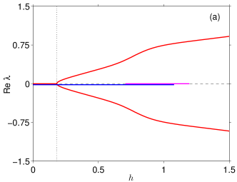
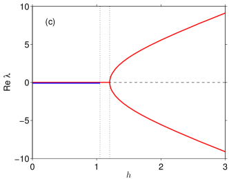
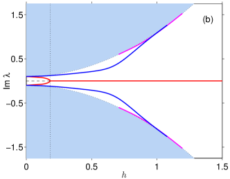
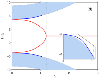
Figure 7: The real and imaginary part of eigenvalues $\lambda$ of the problem (20) as a function of the normalised amplitude $h$. In (a)-(b), $\sigma=0.1$; in (c)-(d), $\sigma=5$. A pair of opposite imaginary eigenvalues $\pm i\omega_{\mathrm{even}}$ bifurcating from the continuous spectrum as $h$ is increased from 0, collides at the origin and diverges to infinities along the positive and negative real axis (shown by the red lines). Also seen are pairs of imaginary eigenvalues $\pm i\omega_{\mathrm{odd}}$ and $\pm i{\tilde{\omega}}_{\mathrm{even}}$ which detach from the continuous spectrum but then immerse back in the continuum (deep blue and pink arcs, respectively.). Note that in (a) and (c), the horizontal segments of the red, blue and pink curves have been shifted away from the $\mathrm{Re}\,\lambda=0$ line for visual clarity. The inset in (d) zooms in on the imaginary eigenvalue as it splits away from the continuum and then returns to it.

Although equations (32)-(33) provide the complete solution to the stability problem of the in-phase soliton, they do not give any insight into the motion of the eigenvalues on the complex plane. Yet the knowledge of stable and unstable eigenvalues can address a number of pertinent questions, in particular classify the type of instability and identify modes of internal oscillation. The aim of this subsection is to consider the eigenvalues: variationally, asymptotically and numerically.

The variational principle (27) gives rise to simple upper and lower bounds of the lowest eigenvalue $-\lambda^{2}$ of the scalar eigenvalue problem (26) (see Appendix E). The two bounds allow one to follow the corresponding pair of opposite symplectic eigenvalues $\pm\lambda$, as $h$ grows from 0 to $\infty$.

For $h$ smaller than $\mathcal{H}_{0}$, the set of symplectic eigenvalues may only consist of pure imaginary pairs $\lambda=\pm i\omega$. We denote $\pm i\omega_{\mathrm{even}}$ the pair with the smallest value of $\omega^{2}$; the notation will become clear later in this subsection. Using (84), the modulus-squared $\omega_{\mathrm{even}}^{2}$ is found to satisfy

$$\omega_{\mathrm{even}}^{2}\leq\sigma(\sigma-2h^{2}).$$ (37)

Recalling that the continuous spectrum of symplectic eigenvalues $\lambda=\pm i\omega$ in (20) occupies the band $(\sigma+h^{2})^{2}\leq\omega^{2}\leq(\sigma+4+h^{2})^{2}$, we observe that the right-hand side in (37) lies below the bottom edge of the continuous spectrum. Hence

$$\omega_{\mathrm{even}}^{2}<(\sigma+h^{2})^{2},\quad h>0.$$ (38)

This implies that the lowest eigenvalue $-\lambda_{\mathrm{even}}^{2}$ cannot bifurcate from the lower edge of the continuum for any finite $h$.

On the other hand, the inequality in (38) may become equality when $h=0$; hence the bifurcation can occur at this point. Equation (86) indicates that for small $h$, the quantity $\omega_{\mathrm{even}}^{2}$ lies above $\sigma(\sigma-3h^{2})$. Taken together with the inequality (37), this fact implies that “the innermost” pair of imaginary eigenvalues (i.e. the pair with the smallest value of $\omega^{2}$) does indeed bifurcate from the continuum at the point $h=0$.

In fact, there are two pairs of pure imaginary eigenvalues, $\lambda=\pm i\omega_{\mathrm{even}}$ and $\lambda=\pm i\omega_{\mathrm{odd}}$, bifurcating from the edges of the continuous spectrum as $h$ is increased from zero. According to the asymptotic analysis of Appendix F, one pair has even and the other one odd eigenfunctions; hence the choice of notation. Equation (93) gives

$$\omega_{\mathrm{even}}=\sigma-1.438h^{2}+O(h^{4}),$$

$$\omega_{\mathrm{odd}}=\sigma+0.685h^{2}+O(h^{4})\ \mbox{as}\ h\to 0.$$

Note that the lowest value of $\omega^{2}$ is provided by the eigenvalue with the even eigenfunction. This explains the choice of notation in (37)-(38).

In the previous subsection we have shown that the pure imaginary pair $\pm i\omega_{\mathrm{even}}$ (the pair with lowest $\omega^{2}$) converges at the origin and splits into the negative and positive real axis as $h$ is increased through the critical value $\mathcal{H}_{0}$, When $h$ grows to infinity, equations (84) and (87) give a corridor for the absolute value of the emerging real pair:

$$\sigma(2h^{2}-\sigma)\leq\lambda_{\mathrm{even}}^{2}\leq\sigma(2h^{2}-\sigma+4-\frac{16}{3}h^{-2}).$$ (39)

Hence, $|\lambda_{\mathrm{even}}|=\sqrt{2\sigma}h+O(h^{-1})$ as $h\to\infty$. The anti-continuum limit (Appendix H) provides a more specific result:

$$|\lambda_{\mathrm{even}}|=\sqrt{2\sigma}\left[h+\left(1-\frac{\sigma}{4}\right)h^{-1}+O(h^{-3})\right].$$

These variational and asymptotic considerations are corroborated by numerical solutions. Figures 7 show the evolution of the imaginary and real parts of eigenvalues as $h$ grows from 0 to large values, with $\sigma$ being fixed. Clearly seen is a pair of imaginary eigenvalues which detaches from the continuous spectrum at $h=0$, moves on to the real axis, and diverges to infinity at a linear rate, as $h\to\infty$.

VI Antiphase soliton

To classify stability of the antiphase solitons, we consider the eigenvalue problem (20) with $\sigma<0$. Unlike equation (20) with $\sigma>0$, this eigenvalue problem is amenable to analytical treatment only in two regions on the $(\sigma,h)$ plane. These are considered in subsections VI.1 and VI.2. For other parameter values we have to rely upon the asymptotic and numerical eigenvalue analysis.

VI.1 Instability against an odd mode

When ${\sigma}<0$, the matrix $L_{-}+\sigma I$ has a negative eigenvalue (equal to $\sigma$). Hence, the lowest value of $-\lambda^{2}$ in the generalised eigenvalue problem (26) cannot be sought as a minimum of the Rayleigh quotient (27) over the entire $\ell^{2}$ space of square-summable bi-infinite sequences. However, when $\sigma>-h^{2}$, we can use the Rayleigh quotient to establish the existence of eigenvalues with odd (antisymmetric) eigenvectors ${\bf g}$: $g_{-n}=-g_{n}$, $n=0,1,2,...$.

Indeed, the spectrum of the infinite matrix $L_{-}$ does not have eigenvalues other than ${\mathscr{E}}_{0}=0$ and a continuous band $h^{2}\leq\mathscr{E}\leq h^{2}+4$. (We have verified this by computing numerical eigenvalues of a large finite truncation of $L_{-}$ over a representative sample of $h$ values between 0 and $\infty$.) The zero eigenvalue corresponds to an even (symmetric) eigenvector ${\bf z}_{0}=\textit{{R}}$. Therefore, the matrix $L_{-}+\sigma I$ with $\sigma>-h^{2}$, is positive definite on the subspace $\mathfrak{S}$ of $\ell^{2}$ consisting of odd sequences $\bf g$. Consequently, the lowest eigenvalue of the generalised problem (26) associated with an odd eigenvector, is given by

$$-\lambda^{2}=\min_{\mathfrak{S}}\frac{\langle{\bf g}|L_{+}+{\sigma}I|{\bf g}\rangle}{\langle{\bf g}|(L_{-}+{\sigma}I)^{-1}|{\bf g}\rangle}.$$ (40)

Let $E_{1}$ denote the second lowest eigenvalue of the matrix $L_{+}$:

$$L_{+}{\bf y}_{1}=E_{1}{\bf y}_{1}.$$

The eigenvalue $E_{1}$ is positive LST ; KK and satisfies $0<E_{1}(h)<h^{2}$. (See Fig.5(a)). The corresponding eigenvector ${\bf y}_{1}$ is odd and renders the quadratic form $\langle{\bf g}|L_{+}+{\sigma}I|{\bf g}\rangle$ minimum in $\mathfrak{S}$. Equation (40) implies then that $-\lambda^{2}$ is positive respectively negative for $E_{1}+\sigma>0$ respectively $E_{1}+\sigma<0$.

In the region $-h^{2}<\sigma<-E_{1}(h)$, the symplectic eigenvalue problem (20) has a pair of real eigenvalues $\pm\lambda$ signifying the instability of the antiphase soliton against an odd mode. As $\sigma$ approaches $-E_{1}(h)$ from below, the two eigenvalues collide at the origin and move onto the imaginary axis. The odd-mode instability is replaced with a mode of internal oscillation.

In terms of the soliton’s amplitude, $A$, the above odd-mode instability region is given by

$$\sqrt{2}(1-\gamma^{2})^{1/4}<A<\mathcal{A}_{1}({\mathfrak{C}},\gamma),$$ (41)

where

$$\mathcal{A}_{1}=\sqrt{{\mathfrak{C}}}\mathcal{H}_{1}\left({2\sqrt{1-\gamma^{2}}}/{{\mathfrak{C}}}\right)$$ (42)

and $h=\mathcal{H}_{1}(|\sigma|)$ is the function inverse to $|\sigma|=E_{1}(h)$. This function is shown in Fig 5(c). The small- and large-$|\sigma|$ behaviour of $\mathcal{H}_{1}(|\sigma|)$ follow from the corresponding asymptotics of the eigenvalue $E_{1}(h)$ (see the Appendix A):

$$\mathcal{H}_{1}=C\ln^{1/2}(|\sigma|^{-1})\ \mbox{as}\ |\sigma|\to 0,$$

$$\mathcal{H}_{1}=|\sigma|^{1/2}+\mathrm{e.s.t.}\ \mbox{as}\ |\sigma|\to\infty.$$ (43)

Here $C$ is a positive constant and $\mathrm{e.s.t.}$ denotes a positive term that is smaller than $|\sigma|^{-n}$ with any $n>0$. The exponential approach of $\mathcal{H}_{1}$ to $|\sigma|^{1/2}$ as $|\sigma|\to\infty$, is clearly visible in Fig. 5(c).

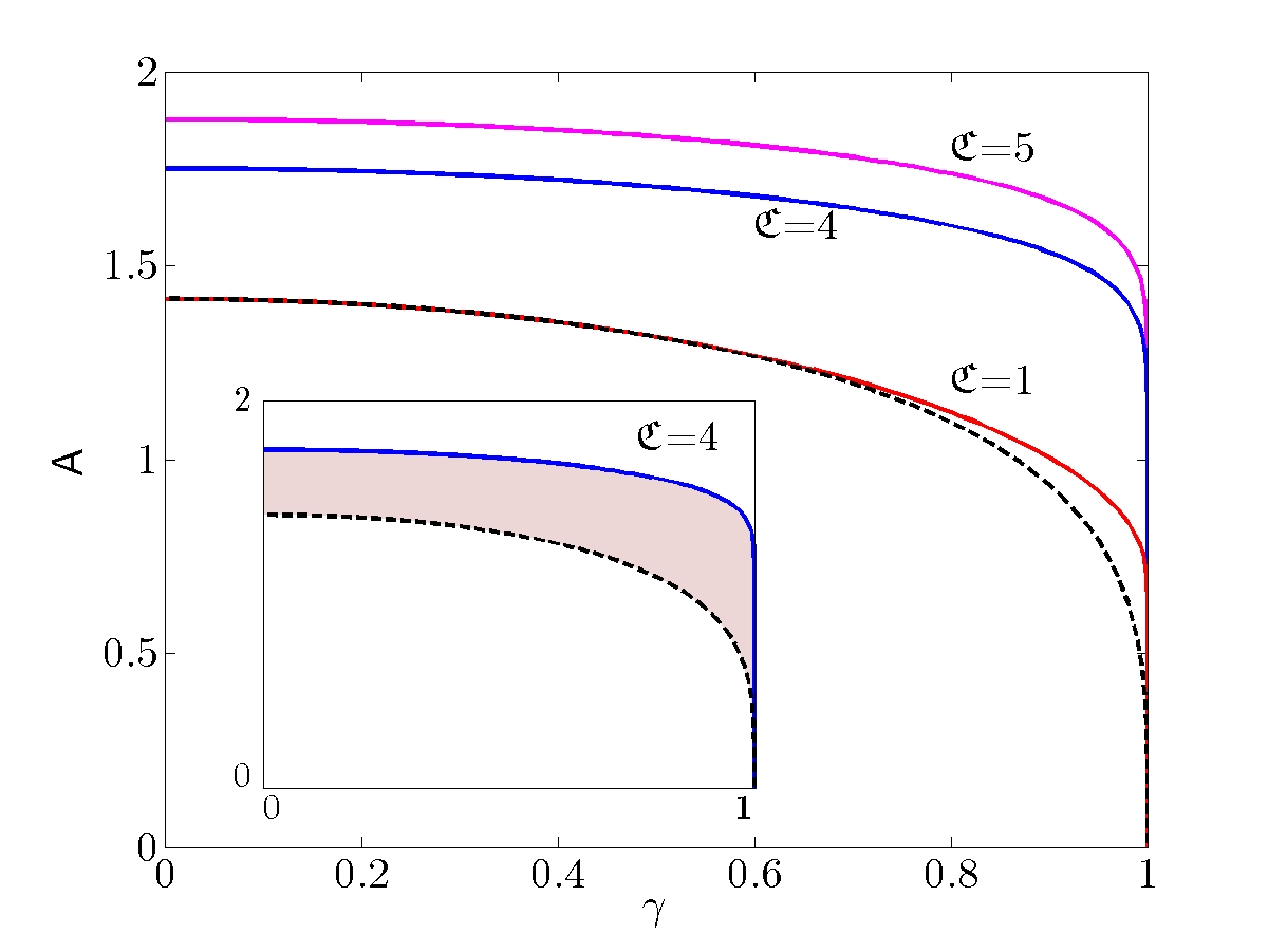
Figure 8: The odd-mode instability band of the atiphase soliton established by the analytical argument of section VI.1. The solid curves demarcate the upper boundary of the full odd-mode instability range, $A=\mathcal{A}_{1}({\mathfrak{C}},\gamma)$, for three different values of ${\mathfrak{C}}$. The dashed curve is given by $A=\sqrt{2}(1-\gamma^{2})^{1/4}$; this curve is common for all $\mathfrak{C}$. (Note that the full odd-mode instability domain extends below the dashed curve.) The instability band (41) is tinted in the inset where only the solid curve with $\mathfrak{C}=4$ has been retained.

The region (41) is displayed in Fig.8 for three values of coupling ${\mathfrak{C}}$: ${\mathfrak{C}}=1$, $4$, and $5$. It is important to emphasise here that the region (41) constitutes only a part of the full odd-mode instability range (namely, the part where this instability can be established by analytical means). While the inequality $A<\mathcal{A}_{1}({\mathfrak{C}},\gamma)$ does demarcate the top boundary of the full odd-mode instability range, the bottom boundary of the full range lies somewhere below the curve $A=\sqrt{2}(1-\gamma^{2})^{1/4}$ and can only be demarcated numerically. (See section VI.6 below.)

As $\mathfrak{C}\to 0$ and hence $|\sigma|\to\infty$, the equation (43) indicates that the width of the instability band (41) becomes exponentially small. (For instance, the solid curve corresponding to ${\mathfrak{C}}=0.1$ would be indistinguishable from the dashed curve in Fig.8.) This argument alone does not yet imply that the full odd-mode instability domain on the $(\gamma,A)$-plane should shrink. However, the numerical study of symplectic eigenvalues demonstrates that this is exactly what happens: the width of the full odd-mode instability domain rapidly approaches zero as ${\mathfrak{C}}\to 0$.

VI.2 Weakly coupled chain away from symmetry breaking: Analytical stability criterion

Defining

$$P_{+}=-(L_{-}+\sigma I),\quad P_{-}=-(L_{+}+\sigma I),$$

the eigenvalue problem (20) is cast in the form

$$\left(\begin{array}[]{cc}P_{+}&0\\ 0&P_{-}\end{array}\right)\left(\begin{array}[]{c}{\bf f}\\ {\bf g}\end{array}\right)=\lambda J\left(\begin{array}[]{c}{\bf f}\\ {\bf g}\end{array}\right).$$ (44)

Let $|\sigma|>4$. If $h^{2}<|\sigma|-4$, or, equivalently,

$$A^{2}<2\sqrt{1-\gamma^{2}}-4{\mathfrak{C}},$$ (45)

both matrices $P_{+}$ and $P_{-}$ are positive definite. Hence the variational principle (27) is valid and the lowest eigenvalue $-\lambda^{2}$ is positive:

$$-\lambda^{2}=\min\frac{\langle{\bf g}|P_{+}|{\bf g}\rangle}{\langle{\bf g}|P_{-}^{-1}|{\bf g}\rangle}>0.$$ (46)

The upshot of this elementary consideration is that if the chain parameters satisfy

$${\mathfrak{C}}<1/2,\quad 0\leq\gamma\leq\sqrt{1-4{\mathfrak{C}}^{2}},$$ (47)

the antiphase soliton has a range of stable amplitudes given by (45).

It is important to emphasise that the region described by the inequalities (47) and (45) constitutes only a part of the full stability domain of the antiphase soliton; see Fig 13(a). The significance of this region lies in the fact that stability is guaranteed by an accurate analytical argument here. Unlike the numerical eigenvalue analysis, this argument would have not missed even a weak instability — if there had been any.

VI.3 Surprising stability of large-amplitude solitons

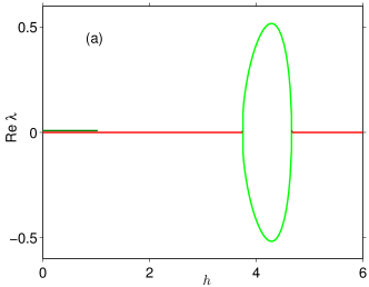
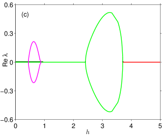
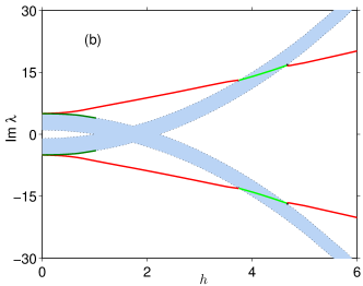
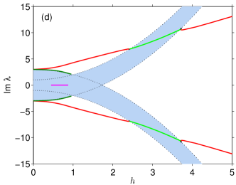
Figure 9: The real (top) and imaginary (bottom) part of the symplectic eigenvalue $\lambda$ as a function of the normalised amplitude $h$. Left column: $\sigma=-5$; right column: $\sigma=-3$. Each of the two red lines in (b,d) follows an imaginary eigenvalue bifurcating from a continuous spectrum band at $h=0$. The eigenvalue grows in absolute value and acquires a real part as it traverses the other continuum band. One more pair of imaginary eigenvalues (shown in dark green) bifurcates from the continuous spectrum at $h=0$ but then returns to the continuum. The pink oval in (c) describes a pair of real eigenvalues.

The two regions (41) and (47),(45) exhaust all parameter values where the stability of the antiphase solitons can be classified using exact analytical criteria. In the complementary part of the parameter space, one has to resort to numerical and asymptotic techniques.

Results of our numerical study of the eigenvalue problem (20) with negative $\sigma$ are summarised in Figs 9 and 10.

A striking difference between these two figures on the one hand — and stability properties of the corresponding continuous system ABSK on the other — is in the discrete soliton stabilisation as its amplitude becomes large enough. (We remind the reader that once the coupling constant ${\mathfrak{C}}$ has been fixed, the amplitude can be represented by the quantity $h=A/\sqrt{{\mathfrak{C}}}$.) Indeed, all we see in Figs 9 and 10 with a sufficiently large $h$ is a pair of opposite pure imaginary eigenvalues. These eigenvalues are given by the power expansion (102) with coefficients as in (104):

$$\lambda=\pm i\sqrt{2|\sigma|}\left[h+\left(1-\frac{\sigma}{4}\right)h^{-1}+O(h^{-3})\right].$$ (48)

As $h$ is decreased from large values, each of the two imaginary eigenvalues seems to collide with the corresponding branch of the continuous spectrum and acquire a real part. A scrutiny of the collision area reveals that the imaginary eigenvalue approaching the continuum collides not with the edge of the continuous-spectrum band itself but with another pure imaginary eigenvalue that bifurcates from the edge just before the collision. The distance in $h$ between the point of bifurcation and point of collision is so short that this second eigenvalue is hardly discernible for large $|\sigma|$ (Fig 9). However it is clearly visible when $|\sigma|$ is chosen smaller than $1$ (Fig 10).

The collision is nothing but the Hamiltonian Hopf bifurcation. It results in a quadruplet of complex eigenvalues $\pm\lambda,\pm\lambda^{*}$. In what follows, the bifurcation value of $h$ is denoted by $\mathcal{H}_{3}(|\sigma|)$. Recalling that $h=A/\sqrt{{\mathfrak{C}}}$ and $\sigma=-2\omega_{0}/{\mathfrak{C}}$, this gives the upper boundary of the soliton instability domain:

$$\mathcal{A}_{3}=\sqrt{\mathfrak{C}}\mathcal{H}_{3}\left(2\sqrt{1-\gamma^{2}}/{\mathfrak{C}}\right),$$ (49)

where the function $\mathcal{H}_{3}(|\sigma|)$ admits a simple asymptote PY :

$$\mathcal{H}_{3}\to 2|\sigma|^{1/2}+\left(\frac{\sqrt{15}}{4}-\frac{1}{2}\right)|\sigma|^{-1/2}+O(|\sigma|^{-3/2})\ \mbox{as}\ |\sigma|\to\infty.$$

The asymptotic behaviour for the upper boundary of the soliton instability domain is then

$$\mathcal{A}_{3}\to 2\sqrt{2}(1-\gamma^{2})^{1/4}\left[1-\frac{1}{8}\left(1-\frac{\sqrt{15}}{2}\right)\frac{{\mathfrak{C}}}{\sqrt{1-\gamma^{2}}}+O\left(\frac{{\mathfrak{C}}^{2}}{1-\gamma^{2}}\right)\right]\ \mbox{as}\ \frac{{\mathfrak{C}}}{\sqrt{1-\gamma^{2}}}\to 0.$$ (50)

VI.4 Small amplitude solitons: stable or long-lived

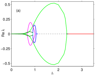
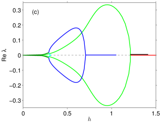
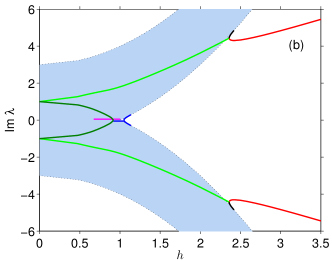
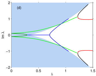
Figure 10: The real and imaginary part of the eigenvalue $\lambda$ of the problem (20) as a function of the normalised amplitude $h$. Left column: $\sigma=-1$; right column: $\sigma=-0.1$. Two light-green curves trace a complex quadruplet with even eigenvectors while the dark-green arc marks complex eigenvalues with odd eigenvectors. As the imaginary parts of the “even” quadruplet emerge from the continuous spectrum, the quadruplet dissociates into two pairs of imaginary eigenvalues described by the black and red curves. The “odd” quadruplet also dissociates as $h$ is increased; the products include two pairs of real eigenvalues shown in light-blue and deep-blue, respectively. The “light-blue” eigenvalues converge on the origin and disappear in the gapless continuous spectrum. The “deep-blue” pair moves away from the origin but then reverses and crosses to the imaginary axis as well. By the time the “deep-blue” doublet reaches the origin, a gap will have opened in the continuous spectrum. The doublet reaches the boundaries of the gap and immerses in the continuum. The pink oval in (a) represents a pair of real eigenvalues with even eigenvectors.

The limit $h\to 0$, with small or finite $|\sigma|$ ($\sigma<0$), is also amenable to asymptotic analysis. See Appendix G and F, respectively. As $h$ grows from zero, either two pairs of pure imaginary or two quadruplets of complex eigenvalues bifurcate from the endpoints of the continuous spectrum (more specifically, from the $\mathrm{Im}\,\lambda=\pm\sigma$ endpoints). Whether the bifurcating eigenvalues have real parts or not, their imaginary parts are given by equations (93) and (96):

$$\mathrm{Im}\,\lambda_{\mathrm{even}}=\pm(\sigma-1.438h^{2})+O(h^{4}/\sigma),$$

$$\mathrm{Im}\,\lambda_{\mathrm{odd}}=\pm(\sigma+0.685h^{2})+O(h^{4}/\sigma).$$

Numerically, the bifurcating imaginary eigenvalues are clearly visible when $|\sigma|>2$. See e.g. Fig 9(b) for $\sigma=-5$ and Fig 9(d) for $\sigma=-3$. When $|\sigma|<2$, by contrast, the point $\mathrm{Im}\,\lambda=\sigma$ — the bottom of the upper band of the continuous spectrum — is embedded in the lower band, which covers the interval $-\sigma-4\leq\mathrm{Im}\,\lambda\leq-\sigma$. (Compare the panel (b) of Fig 4 with panels (c) and (d).) In this case, the bifurcating eigenvalues with small or zero real parts are concealed in the continuum bands and are much harder to track.

The asymptotic analysis of the problem (20) with a negative $\sigma$ of order one, provides no clue on whether the eigenvalues bifurcating from the edge of the continuum have real parts or not. The only conclusion one can draw from it is that if an eigenvalue has a nonzero real part, this real part will have to lie beyond all orders of $h^{n}$. (The proof of this fact is in Appendix F.) The asymptotic argument in Appendix G is of more use here as it guarantees the existence of an (exponentially small) real part when $|\sigma|$ is small enough. Also useful is the variational principle of section VI.2; this principle ensures that all eigenvalues of the operator (25) with small $h$ are pure imaginary if $|\sigma|>4$. Taken together, these two considerations suggest that there is a critical value $\sigma_{c}$ ($|\sigma_{c}|\leq 4$) such that the bifurcating eigenvalues acquire an exponentially small real part when $|\sigma|<|\sigma_{c}|$ but remain pure imaginary when $|\sigma|\geq|\sigma_{c}|$.

Our numerics support this conjecture and indicate that $\sigma_{c}$ is close to $-1.96$. For all $|\sigma|\geq 1.96$ that we have examined, the two pairs of bifurcating eigenvalues were found to be pure imaginary. They only develop nonzero real parts once their imaginary parts collide with the continuous spectrum bands at some finite $h$. (Note the square-root dependence of $\mathrm{Re}\,\lambda$ on $h$ in the vicinity of the collision point in Fig 9 (a) and (c).)

When $|\sigma|<1.96$, by contrast, eigenvalues corresponding to small $h$ exhibit nonzero real parts. In this case, the shape of the $\mathrm{Re}\,\lambda(h)$ curve is indicative of an exponential decay as $h\to 0$. See Fig 10 (a,c) and note the difference in the behaviour of the curve from the square-root law near the collision point in Fig 9 (a,c).

The proximity of the critical value $\sigma_{c}$ to $-2$ sheds some light on the source of the weak oscillatory instability. Unlike the case $|\sigma|>2$, the imaginary parts of the bifurcating eigenvalues of the operator (25) with $|\sigma|\leq 2$ are embedded in the continuous spectrum right from the moment they were born, that is, as early as at $h=0$. Consequently, the emergence of a nonzero real part is due to the resonance between the frequency corresponding to the imaginary part of the bifurcating eigenvalue, and frequencies of the continuous spectrum.

In summary, the small-amplitude antiphase solitons are stable if $|\sigma|\geq 1.96$ or, equivalently, when $\mathfrak{C}<1.02$ and $\gamma\leq\sqrt{1-0.96\mathfrak{C}^{2}}$. Conversely, in the region $|\sigma|<1.96$ (that is, when $\mathfrak{C}>1.02$ and $0\leq\gamma\leq 1$ or when $\mathfrak{C}\leq 1.02$ and $\gamma>\sqrt{1-0.96\mathfrak{C}^{2}}$), these solitons manifest weak instability with growth rate exponentially small in $h$. In the latter case, solitons with sufficiently small amplitudes live long enough to be deemed practically stable.

VI.5 Weakly coupled chain away from $\mathcal{PT}$-symmetry breaking: disjoint stability domain

When the structural parameter $|\sigma|$ is greater than $4$ (that is, when ${\mathfrak{C}}<1/2$ and $0\leq\gamma\leq\sqrt{1-4{\mathfrak{C}}^{2}}$), the complex quadruplet associated with the continuous-band crossing is the only set of unstable eigenvalues that arise as $h$ varies from $0$ to $\infty$. See Fig 9 (a,b). In this case, as $h$ is decreased from $\mathcal{H}_{3}$ (the point of collision with the “inner” edge of the continuum), the imaginary part of the eigenvalue travels through the continuous band and crosses through its “outer” edge. At the point where the imaginary part emerges from the continuum, the real part of the eigenvalue appears to vanish. We denote this point by $h=\mathcal{H}_{2}(|\sigma|)$ and the corresponding value of the amplitude by $\mathcal{A}_{2}$:

$$\mathcal{A}_{2}=\sqrt{\mathfrak{C}}\mathcal{H}_{2}\left({2\sqrt{1-\gamma^{2}}}/{\mathfrak{C}}\right).$$ (51)

The function $\mathcal{H}_{2}$ admits a simple asymptotic representation PY :

$$\mathcal{H}_{2}\to 2|\sigma|^{1/2}-\left(\frac{\sqrt{15}}{4}+\frac{1}{2}\right)|\sigma|^{-1/2}+O(|\sigma|^{-3/2})\ \mbox{as}\ |\sigma|\to\infty.$$

This gives an asymptotic expression for the lower boundary of the instability region:

$$\mathcal{A}_{3}\to 2\sqrt{2}(1-\gamma^{2})^{1/4}\left[1-\frac{1}{8}\left(1+\frac{\sqrt{15}}{2}\right)\frac{{\mathfrak{C}}}{\sqrt{1-\gamma^{2}}}+O\left(\frac{{\mathfrak{C}}^{2}}{1-\gamma^{2}}\right)\right]\ \mbox{as}\ \frac{{\mathfrak{C}}}{\sqrt{1-\gamma^{2}}}\to 0.$$ (52)

As with the inner-edge crossing, the numerical scrutiny confirms that this process is more complex than it seems. It involves two pairs of complex eigenvalues which converge on two opposite points on the imaginary axis and dissociate into two pure imaginary pairs. After that, one pair of opposite imaginary eigenvalues immerses in the continuum whereas the other pair moves away from it. The interval of $h$ where two imaginary pairs coexist is so tiny that the complex eigenvalues appear to be stripped of their real parts as soon as the imaginary parts have emerged out of the continuum.

While considering diagrams pertaining to large $|\sigma|$, a natural question concerns the odd-mode instability of section VI.1. The domain of the odd-mode instability includes (though is not limited to) the interval $|\sigma|^{1/2}<h<\mathcal{H}_{1}(|\sigma|)$. Why is this instability not manifest in the $\lambda(h)$ dependencies with large $|\sigma|$ (Fig.9)?

The answer is that since the function $\mathcal{H}_{1}(|\sigma|)$ approaches $|\sigma|^{1/2}$ exponentially fast as $|\sigma|$ grows, the above interval of unstable $h$ shrinks and becomes indiscernible (see Fig 5(c)). Furthermore, the numerical analysis indicates that the full odd-mode instability domain also shrinks as $|\sigma|$ grows. Therefore, although the solitons with large negative $\sigma$ are prone to the odd-mode instability, the interval of “unstable” $h$ is minuscule.

The shrinking of the odd-mode instability band (41) as the coupling ${\mathfrak{C}}$ is reduced, is clearly visible in Fig 8. In the weakly coupled chain of waveguides, the numerical detection of this band is only feasible if $\gamma$ is close to 1 (so that the argument of $\mathcal{H}_{1}$ in (42) is small enough).

Our conclusions can be summarised as follows. The stability domain in a chain with ${\mathfrak{C}}<1/2$ and $0\leq\gamma\leq\sqrt{1-4{\mathfrak{C}}^{2}}$ consists of two disjoint parts. The soliton is unstable if its amplitude falls between $\mathcal{A}_{2}$ and $\mathcal{A}_{3}$, and stable when $A$ lies outside this band. Here $\mathcal{A}_{2}$ is as in (51) and $\mathcal{A}_{3}$ as in (49), with the corresponding asymptotic behaviours given by (52) and (50), respectively. (There is also a narrow band of the odd-mode instability immersed in the stability domain but it is of little significance due to its exponentially small width.)

The disjoint stability domain on the $(\gamma,A)$-plane is illustrated in Fig 13(a). The dashed curve in this panel demarcates the region where the soliton’s stability has been established using the variational principle (46). It is obvious that the analytical argument secures only a small portion of the full stability domain.

VI.6 Numerical eigenvalue trajectories

While the complex quadruplet crossing the continuous spectrum band is the only set of unstable eigenvalues for $|\sigma|>4$, chains with smaller values of $|\sigma|$ feature several more instabilities. This subsection summarises results of our numerical study of the problem (20) with $0<|\sigma|<4$. As before in this section, we keep $\sigma<0$.

The complex quadruplet exhibited by the operator (25) with $|\sigma|>4$ persists for $|\sigma|<4$. In Figs 9 and 10 the trajectories of complex eigenvalues constituting the quadruplet in question, are delineated in light green. Similarly to the $|\sigma|>4$ scenario, the quadruplet is born in a Hamiltonian Hopf bifurcation as $h$ is decreased through the point $\mathcal{H}_{3}(|\sigma|)$. A further decrease of $h$ with a fixed $|\sigma|\geq 1.96$ brings about an inverse Hopf bifurcation, at the point $h=\mathcal{H}_{2}(|\sigma|)$, where the quadruplet dissociates into two opposite pairs of imaginary eigenvalues. When $|\sigma|<1.96$, by contrast, the quadruplet persists over the entire interval $0<h\leq\mathcal{H}_{3}$. (Its asymptotic behaviour as $h\to 0$ was discussed in section VI.4.)

We note that the eigenvectors associated with the “light-green” quadruplet, are symmetric (that is, even in $n$). The left-right symmetry of the eigenvectors distinguishes this quadruplet from another quadruplet of complex eigenvalues that is shown in dark green in Fig 10. The eigenvectors of the “dark-green” eigenvalues are antisymmetric (odd in $n$).

The left-right symmetry of the eigenvectors gives rise to a symmetric instability growth. Fig 11 illustrates two possible outcomes of the decay of the antiphase soliton unstable against the “light-green” complex quadruplet. In Fig 11 (a) the growing oscillations culminate in the exponential blow-up of the soliton. In Fig 11 (b), the oscillatory instability transforms the soliton into a breather — a spatially localised structure with a steadily oscillating amplitude and width.

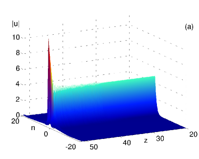
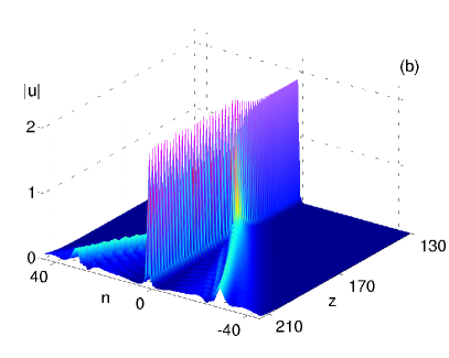
Figure 11: The blow-up of the antiphase soliton (a) and formation of a breather (b). In (a), the parameters of the lattice are ${\mathfrak{C}}=17.32$, $\gamma=0.5$, and the soliton’s initial amplitude is $A=5.05$. These values correspond to the point $h=1.21$ in Fig 10 (c,d) (where $\sigma=-0.1$). In (b), the lattice has ${\mathfrak{C}}=0.366$ and $\gamma=0.4$; the initial amplitude of the decaying antiphase soliton is $A=2.51$. These parameters correspond to a point $h=4.15$ in Fig 9 (a,b) (where $\sigma=-5$). The instability responsible for the evolution shown in (a) and (b), is due to the complex quadruplet marked by the light green lines in Fig 10 and Fig 9, respectively.

The pink loop in Fig 9(c) and 10(a) describes a pair of opposite real eigenvalues (also with even eigenvectors). These hail from the imaginary axis: as $h$ is decreased, a pair of pure imaginary eigenvalues bifurcates from the continuous spectrum, converges at the origin and moves on to the real axis. As $h$ is decreased further, the eigenvalues reach their maximum absolute value and then return to the origin.

The “pink loop” is present in all diagrams with $|\sigma|$ between $4$ and approximately $0.4$. When $|\sigma|<1.96$, these real eigenvalues coexist with the complex quadruplet and do not produce any further reduction of the soliton stability domain. The stability domain has a simple structure in this case: the soliton is stable when $h>\mathcal{H}_{3}(|\sigma|)$ and unstable otherwise.

The inequality $|\sigma|<1.96$ describes a union of two regions on the $(\mathfrak{C},\gamma)$-plane:

$$\mathfrak{C}>1.02,\quad 0\leq\gamma<1;$$ (53a)

$$\mathfrak{C}\leq 1.02,\quad\gamma>\sqrt{1-0.96\mathfrak{C}^{2}}.$$ (53b)

In either case the soliton stability domain is connected: $A\geq\mathcal{A}_{3}(\mathfrak{C},\gamma)$, where $\mathcal{A}_{3}$ is as in (49). See Figs 13(a,b,c).

The real even (“pink”) mode becomes more significant for $|\sigma|$ between $1.96$ and $4$. When $|\sigma|$ is in this range, we have two separate intervals of “unstable” values of $h$: the interval $\mathcal{H}_{2}(|\sigma|)<h<\mathcal{H}_{3}(|\sigma|)$ bearing the complex quadruplet, and an additional interval $\mathcal{H}_{4}(|\sigma|)<h<\mathcal{H}_{5}(|\sigma|)$, with $\mathcal{H}_{5}<\mathcal{H}_{2}$, hosting the “pink” pair of real eigenvalues.

Unlike the oscillatory instability discussed above, the monotonic growth associated with the real mode cannot give rise to any breathing structures. A typical evolution is illustrated in Fig 12 (a). The unstable antiphase soliton sheds some power and transforms into a stable soliton of the same variety.

The inequality $1.96\leq|\sigma|<4$ selects two more regions on the $(\mathfrak{C},\gamma)$-plane:

$$\mathfrak{C}\leq 1/2,\quad\sqrt{1-4\mathfrak{C}^{2}}<\gamma\leq\sqrt{1-0.96\mathfrak{C}^{2}};$$ (54a)

$$1/2<\mathfrak{C}<1.02,\quad\gamma\leq\sqrt{1-0.96\mathfrak{C}^{2}}.$$ (54b)

Each of these two regions features two non-overlapping intervals of unstable amplitudes, $\mathcal{A}_{4}<A<\mathcal{A}_{5}$ and $\mathcal{A}_{2}<A<\mathcal{A}_{3}$, where

$$\mathcal{A}_{n}=\sqrt{\mathfrak{C}}\mathcal{H}_{n}\left({2\sqrt{1-\gamma^{2}}}/{\mathfrak{C}}\right),\quad n=2,3,4,5.$$ (55)

Two corridors of instability are clearly visible in the left part of Fig 13(b) and middle section of Fig 13(a).

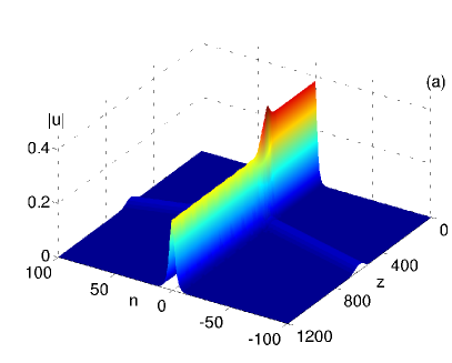
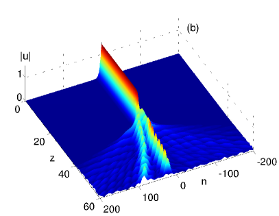
Figure 12: Two more outcomes of the antiphase soliton instability growth. (a): The instability caused by a real eigenvalue with an even eigenvector. In Figs 9(c,d) and 10(a,b), this eigenvalue is marked by the pink line. The unstable soliton emits a pair of small-amplitude solitons with opposite velocities and transforms into a (stationary) antiphase soliton of smaller amplitude. Here the lattice coupling is ${\mathfrak{C}}=0.3$, gain-loss coefficient $\gamma=0.93$ and the initial soliton’s amplitude $A=0.37$. (These parameters fall into the “white fang” region in Fig 13(a).) The emerging soliton has $A=0.26$. (This belongs in the green region just under the white fang.) (b): The joint effect of the real eigenvalue with an odd eigenvector (the deep-blue line in Fig 10) and the complex quadruplet (light-green lines in Fig 10). The soliton breaks into an eccentric bunch of breathers. Here ${\mathfrak{C}}=19.9$, $\gamma=0.1$, and $A=1.41$. These values correspond to the point $h=0.32$ in Fig 10(c,d) (where $\sigma=-0.1$).

Another instability that has a sizeable domain in chains with $|\sigma|<2$, is due to a pair of real eigenvalues with odd eigenvectors. The inequality $|\sigma|^{1/2}<h<\mathcal{H}_{1}(|\sigma|)$ of section VI.1 defines the upper part of the odd-mode instability domain; the lower part has to be determined numerically. The trajectory of the odd-mode eigenvalues on the $(h,\mathrm{Re}\,\lambda)$-plane is described by the deep-blue curve in Fig 10 (a,c). Like the even real mode discussed in the previous paragraphs, this pair of real eigenvalues is born as an imaginary pair which bifurcates from the continuous spectrum. [See the deep-blue curves in Fig 10 (b,d).] As $h$ is decreased to the value of $\mathcal{H}_{1}(|\sigma|)$, the two imaginary eigenvalues collide and move to the real axis — in agreement with the variational argument of section VI.1.

What the variational principle is powerless to determine though, is the trajectory of these eigenvalues on the complex plane as $h$ is decreased below $|\sigma|^{1/2}$. The numerical analysis, on the other hand, reveals the arrival of yet another pair of real eigenvalues from the imaginary axis via the origin (shown in light blue in Fig 10 (a,c)). Like the “dark-blue” eigenvalues, the newly born pair has odd eigenvectors. At some $h<|\sigma|^{1/2}$, the “light-blue” and “deep-blue” eigenvalues collide, pairwise, and emerge into the complex plane.

The evolution of the resulting complex quadruplet depends on whether $|\sigma|$ is greater or smaller than 2. When $|\sigma|<2$, the quadruplet persists all the way to $h=0$, with the real parts of the complex eigenvalues decaying to zero. (See the stiletto-shaped dark-green curves in Fig 10(a)). According to section VI.4, the decay is exponentially fast as $h\to 0$. When $2<|\sigma|<4$, the complex eigenvalues converge, pairwise, at two opposite points on the imaginary axis outside the continuous spectrum band. After that one pair of imaginary eigenvalues immerses in the continuum while the other one remains outside the band, approaching the band edges only as $h\to 0$. (See the dark-green arcs in Fig 9(d).)

Regardless of the value of $\sigma$, the point $h=\mathcal{H}_{1}(|\sigma|)$ where the odd-mode instability sets in, is to the left of $\mathcal{H}_{3}(|\sigma|)$, the Hamiltonian Hopf bifurcation point where the even-mode (“light-green”) complex quadruplet is born. When $|\sigma|<2$, the even-mode quadruplet persists as $h$ is decreased from $\mathcal{H}_{3}$ to $0$. Accordingly, in this $\sigma$ range the “deep-blue” real eigenvalues and their descendent “dark-green” complex quadruplet coexist with the complex quadruplet shown in light green. Therefore although the odd-mode instability is detectable in direct computer simulations of the antiphase soliton, its presence does not affect the soliton stability domain on the $(\gamma,A)$-plane.

Due to the coexistence of the real eigenvalues and the complex quadruplet, the odd-mode monotonic instability and the even-mode oscillatory one, develop simultaneously. A typical outcome of the soliton decay in the parameter range with $|\sigma|<2$ is depicted in Fig 12 (b). The antiphase soliton breaks into an asymmetric assembly of two or more travelling breathers.

When $2<|\sigma|<4$, the point $h=\mathcal{H}_{1}(|\sigma|)$ is to the left of $\mathcal{H}_{2}(|\sigma|)$, the lower boundary of the “light-green” quadruplet domain of existence. When $|\sigma|$ falls in this range, the intervals of the odd- and even-mode instability do not overlap. However the odd-mode instability band is so narrow here that this instability would be hard to observe in computer simulations of the soliton. The odd instability band is marked as a white line in Fig 13(a).

We close this subsection by acknowledging an earlier numerical study of the eigenvalue problem (20). The authors of Ref PY computed eigenvalues for three fixed values of $h$ ($h=0.50,0.71$ and $3.16$) and varied $\sigma$. This is obviously not equivalent to the approach of the present paper where we fix $\sigma$ and vary $h$.

VII Concluding remarks

VII.1 Conclusions

In this paper we have considered stability of the site- and bond-centred solitons in the chain of $\mathcal{PT}$-symmetric dimers with gain and loss. Both classes of solitons come in two varieties: the in-phase and the antiphase solitons. Our principal results are as follows.

1. We have shown that small perturbations about the soliton can be decomposed into a part tangent to the conservative invariant manifold containing the soliton, and a part that is transversal to that manifold. This decomposition proves instability of both varieties of the bond-centred solitons, for all amplitudes and all values of the chain parameters.

2. We have demonstrated that stability properties of a site-centred soliton with amplitude $A$ in the chain with the inter-dimer coupling ${\mathfrak{C}}$ and gain-loss coefficient $\gamma$, are completely determined just by two combinations of $A$, ${\mathfrak{C}}$ and $\gamma$. These are the structural parameter $\sigma=\pm 2\sqrt{1-\gamma^{2}}/{\mathfrak{C}}$ (where the top and bottom sign correspond to the in-phase and antiphase soliton, respectively) and the normalised amplitude $h=A/\sqrt{{\mathfrak{C}}}$.

3. We have proved that the in-phase site-centred soliton is stable if its amplitude lies below a threshold value (33) and unstable otherwise. A simple upper bound for the threshold, equation (34), has been established and its explicit expressions in the small-coupling limit (${\mathfrak{C}}/\sqrt{1-\gamma^{2}}\to 0$) and in the limit where $\sqrt{1-\gamma^{2}}/{\mathfrak{C}}\to 0$ have been provided. (See equations (36) and (35), respectively.) The lowest threshold occurs in chains where the value of the dimer-to-dimer coupling ${\mathfrak{C}}$ is close to the value of the gain-to-loss coupling within each dimer.

4. With regard to the stability of the site-centered antiphase soliton, we have identified three characteristic coupling ranges: (a) $\mathfrak{C}<1/2$, (b) $1/2<\mathfrak{C}<1.02$, and (c) $\mathfrak{C}>1.02$.

4(a). In the weak-coupling range ($\mathfrak{C}<1/2$), the structure of the stability domain depends on whether the gain-loss coefficient (i) is smaller than $\sqrt{1-4{\mathfrak{C}}^{2}}$; (ii) falls between $\sqrt{1-4{\mathfrak{C}}^{2}}$ and $\sqrt{1-0.96{\mathfrak{C}}^{2}}$, or (iii) is greater than $\sqrt{1-0.96{\mathfrak{C}}^{2}}$. (i) When $\gamma$ lies below $\sqrt{1-4{\mathfrak{C}}^{2}}$, the soliton is unstable if its amplitude satisfies $\mathcal{A}_{2}<A<\mathcal{A}_{3}$ and stable otherwise. As $\mathfrak{C}/\sqrt{1-\gamma^{2}}\to 0$, the functions $\mathcal{A}_{2}(\mathfrak{C},\gamma)$ and $\mathcal{A}_{3}(\mathfrak{C},\gamma)$ are given by the asymptotic expressions (52) and (50), respectively. Otherwise $\mathcal{A}_{2}$ and $\mathcal{A}_{3}$ are as in (51) and (49), with $\mathcal{H}_{2}$ and $\mathcal{H}_{3}$ determined numerically. (ii) When $\gamma$ falls between $\sqrt{1-4{\mathfrak{C}}^{2}}$ and $\sqrt{1-0.96{\mathfrak{C}}^{2}}$, there are two instability bands: $\mathcal{A}_{2}<A<\mathcal{A}_{3}$ and $\mathcal{A}_{4}<A<\mathcal{A}_{5}$, with $\mathcal{A}_{n}$ as in (55) and $\mathcal{H}_{n}$ determined numerically. (iii) When $\gamma$ is greater than $\sqrt{1-0.96\mathfrak{C}^{2}}$, the amplitudes above $\mathcal{A}_{3}$ are stable and those below $\mathcal{A}_{3}$ unstable.

In addition to the above one or two instability bands, we need to note an extremely thin corridor of odd-mode instability that crosses the soliton stability domain when ${\mathfrak{C}}<1/2$ and $\gamma<\sqrt{1-0.96{\mathfrak{C}}^{2}}$. The upper part of this corridor is described by the inequalities in (41), with the corresponding asymptotic expressions as in (43).

4(b). In the middle range ($1/2<\mathfrak{C}<1.02$), the stability criteria depend on whether the gain-loss coefficient is greater or smaller than $\sqrt{1-0.96\mathfrak{C}^{2}}$. When $\gamma<\sqrt{1-0.96\mathfrak{C}^{2}}$, the soliton is unstable if its amplitude falls in either of two bands, $\mathcal{A}_{2}<A<\mathcal{A}_{3}$ or $\mathcal{A}_{4}<A<\mathcal{A}_{5}$ — and stable otherwise. When $\gamma>\sqrt{1-0.96\mathfrak{C}^{2}}$, the amplitudes above the threshold value $\mathcal{A}_{3}$ are stable and those below the threshold are unstable. The boundaries $\mathcal{A}_{n}({\mathfrak{C}},\gamma)$ ($n=2,...,5$) are as in (55), with the functions $\mathcal{H}_{n}$ being determined numerically.

4(c). In the strong coupling range ($\mathfrak{C}>1.02$), solitons with amplitudes above $\mathcal{A}_{3}$ are stable and those below $\mathcal{A}_{3}$ unstable. The threshold amplitude is given by equation (49) where the function $\mathcal{H}_{3}(|\sigma|)$ is determined numerically.

4(d) In the parameter regimes where the small-amplitude solitons are unstable (in the strong-coupling range $\mathfrak{C}>1.02$ and in the range $\mathfrak{C}<1.02$ with $\gamma>\sqrt{1-0.96{\mathfrak{C}}^{2}}$), the instability growth rate becomes exponentially small as the soliton’s amplitude tends to zero. Hence unstable solitons with small amplitudes can live long enough to be regarded as practically stable.

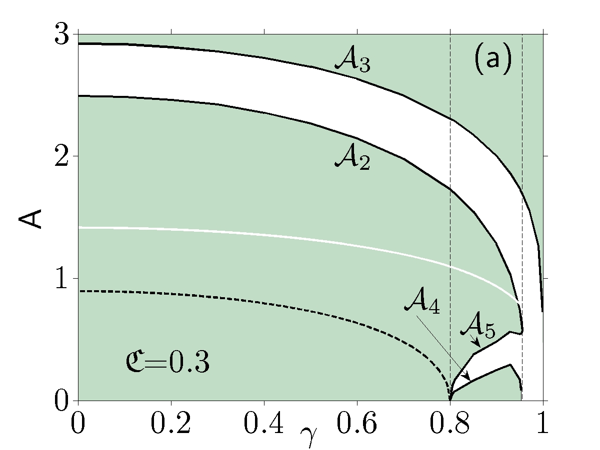
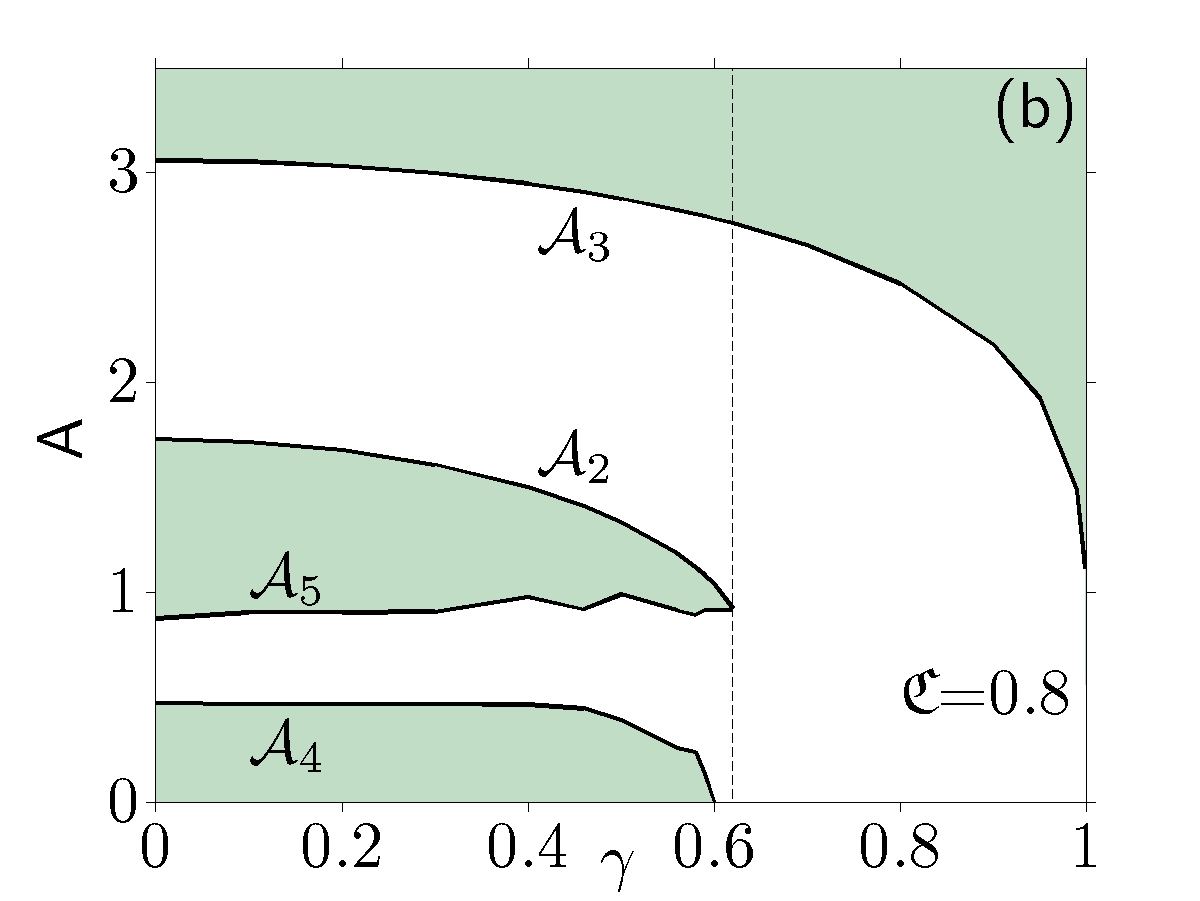
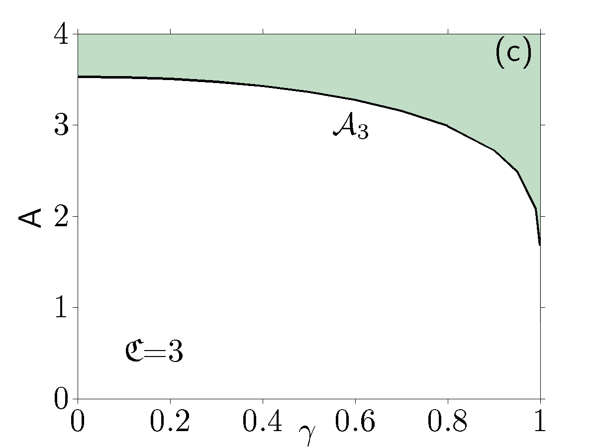
Figure 13: Stability domain of the antiphase soliton in the chain with ${\mathfrak{C}}<1/2$ (a), $1/2<{\mathfrak{C}}<1.02$ (b) and ${\mathfrak{C}}>1.02$ (c). The stability domain is tinted green while corridors of instability are left blank. The left vertical line in (a) is given by $\gamma=\sqrt{1-4{\mathfrak{C}}^{2}}$ and the right one by $\gamma=\sqrt{1-0.96{\mathfrak{C}}^{2}}$. The vertical line in (b) is $\gamma=\sqrt{1-0.96{\mathfrak{C}}^{2}}$.
Panel (a): In the interval $0\leq\gamma\leq\sqrt{1-4{\mathfrak{C}}^{2}}$, stable amplitudes lie on each side of the band $\mathcal{A}_{2}<A<\mathcal{A}_{3}$. This corridor continues into the interval $\sqrt{1-4{\mathfrak{C}}^{2}}<\gamma\leq\sqrt{1-0.96{\mathfrak{C}}^{2}}$, where it is joined by the second instability band, $\mathcal{A}_{4}<A<\mathcal{A}_{5}$. In the interval $\sqrt{1-0.96{\mathfrak{C}}^{2}}<\gamma<1$, stable amplitudes lie only above $\mathcal{A}_{3}$. What looks like a white line through the stability domain is a very narrow corridor of the odd-mode instability. The upper boundary of this band is given by $\mathcal{A}_{1}(\gamma)$; the lower boundary is determined numerically. The black dashed curve is given by (45); it bounds the region where the soliton is stable due to a rigorous analytical argument.
Panel (b): When $\gamma\leq\sqrt{1-0.96{\mathfrak{C}}^{2}}$, there are two instability bands: $\mathcal{A}_{4}<A<\mathcal{A}_{5}$ (lower) and $\mathcal{A}_{2}<A<\mathcal{A}_{3}$ (upper band). In the interval $\sqrt{1-0.96{\mathfrak{C}}^{2}}<\gamma<1$, stable amplitudes lie only above $\mathcal{A}_{3}$.
Panel (c): stable amplitudes lie only above $\mathcal{A}_{3}(\gamma)$.

VII.2 Comparison with earlier work

It is instructive to compare our approach and conclusions with those of earlier authors who performed asymptotic analysis in the ${\mathfrak{C}},\gamma\to 0$ limit Susanto and studied soliton stability numerically SMDK ; Susanto .

What we see as an advantage of our approach, is a particular choice of variables that leads to an eigenvalue problem in triangular form (see equations (11) and (18)). The eigenvectors of the triangular matrices admit a natural decomposition into two disjoint classes: the eigenvectors that belong to the scalar reduction of the two-component nonlinear Schrödinger equation (1) and eigenvectors that lie outside the reduction manifold.

This decomposition alone was sufficient for us to prove the instability of all bond-centred solitons, regardless of their amplitude and irrespective of the ${\mathfrak{C}}$ and $\gamma$ parameters of the chain. In contrast, the earlier approaches could only establish the instability of the bond-centred soliton in the ${\mathfrak{C}}\to 0$, $\gamma\to 0$ limit Susanto — and for several isolated parameter triplets that were examined numerically SMDK ; Susanto . Numerical methods require particular caution as they may not be accurate enough to discern small real parts of eigenvalues. This may mislead one into thinking that a weakly unstable soliton is stable (as in the case of the in-phase bond-centred soliton with large ${\mathfrak{C}}$ Susanto .)

In the case of the site-centred soliton, the above decomposition reduces the eigenvalue problem to the form familiar from the theory of the scalar nonlinear Schrödinger equation. This reduction allowed us to use the standard analytical methods for the (discrete) Schrödinger operators. The advantage of halving the dimension of the vector space extends beyond the availability of analytics though. In particular, it simplifies power expansions in the anticontinuum limit where, unlike Susanto , we did not have to assume that $\gamma$ is small.

Another difference between our approach and previous work is that we recognise that the stability properties of the soliton with amplitude $A$ in the chain with coupling ${\mathfrak{C}}$ and gain-loss coefficient $\gamma$, are completely determined just by two combinations of these three parameters. Letting $h=A/\sqrt{{\mathfrak{C}}}$ and $|\sigma|=2\sqrt{1-\gamma^{2}}/{\mathfrak{C}}$ vary over their respective domains, we cover the entire $(A,{\mathfrak{C}},\gamma)$ space.

Our numerical results on the site-centred solitons in the limit ${\mathfrak{C}}\to 0$, $\gamma\to 0$, are in agreement with those of Susanto . On the other hand, the eigenvalue trajectories of the site-centred antiphase soliton with larger ${\mathfrak{C}}$ or $\gamma$ close to 1 — the situation unexplored in Susanto — are found to be much more complex than in the ${\mathfrak{C}},\gamma\to 0$ limit.

Appendix A The negative eigenvalue of operator $L_{+}$ — upper bound

The discrete eigenvalues of the infinite-dimensional matrix (21), $E_{0}$ and $E_{1}$, play a special role in our stability analysis. Unlike the eigenvalues of the corresponding differential operator in ABSK , the matrix eigenvalues do not admit analytic expressions. In this Appendix, we derive a simple upper bound on the lower eigenvalue ($E_{0}$) valid for all $0<h<\infty$.

The derivation starts with the scalar equation (7). Multiplying it with ${\mathcal{R}}_{n}$ and summing over $n$, we obtain

$$2S_{4}-S_{2}=h^{-2}\sum({\mathcal{R}}_{n+1}-{\mathcal{R}}_{n})^{2},$$ (56)

where

$$S_{2}=\sum{\mathcal{R}}_{n}^{2},\quad S_{4}=\sum{\mathcal{R}}_{n}^{4}.$$ (57)

Eq.(56) implies

$$S_{4}\geq\frac{1}{2}S_{2}.$$ (58)

Next, noting that

$$(L_{+})_{nm}=(L_{-})_{nm}-4h^{2}{\mathcal{R}}_{n}^{2}\delta_{mn},$$ (59)

and that ${\mathcal{R}}_{n}$ is the null eigenvector of the matrix $L_{-}$, we have

$$\sum_{n,m}{\mathcal{R}}_{n}(L_{+})_{nm}{\mathcal{R}}_{m}=-4h^{2}S_{4}.$$

Using the inequality (58), this gives

$$\sum_{n,m}{\mathcal{R}}_{n}(L_{+})_{nm}{\mathcal{R}}_{m}\leq-2h^{2}S_{2}.$$ (60)

The lowest eigenvalue of the matrix $L_{+}$ is given by the minimum of the Rayleigh quotient

$$E_{0}=\min_{\bf y}\frac{\sum_{n,m}y_{n}(L_{+})_{nm}y_{m}}{\sum_{n}y_{n}^{2}}.$$

Letting here $y_{n}={\mathcal{R}}_{n}$ and using (60), we obtain an upper bound on the lowest eigenvalue:

$$E_{0}\leq-2h^{2}.$$ (61)

Appendix B The negative eigenvalue of $L_{+}$ in the continuum limit

In this and the next appendix, we establish the asymptotic behaviour of the discrete eigenvalues $E_{0}$ and $E_{1}$ as $h\to 0$. Although (21) is exactly the matrix arising in the linearisation of the scalar discrete nonlinear Schrödinger soliton, these results are not in the existing literature on the subject.

In the limit $h\to 0$, the site-centred soliton solution of equation (7) can be sought as $\mathcal{R}_{n}=\mathcal{R}(X_{n})$, where $\mathcal{R}(X)$ is a continuous function of its argument, and $X_{n}=nh$. The function $\mathcal{R}(X)$ satisfies

$$-2\sum_{\alpha=0}^{\infty}\frac{h^{2\alpha}}{(2\alpha+2)!}\frac{d^{2\alpha+2}\mathcal{R}}{dX^{2\alpha+2}}+\mathcal{R}-2\mathcal{R}^{3}=0,$$ (62)

and can be easily constructed as a power expansion

$$\mathcal{R}=\sum_{\alpha=0}^{\infty}\mathcal{R}^{(\alpha)}h^{2\alpha}+\mathrm{e.s.t.}$$ (63)

Here $\mathrm{e.s.t.}$ stands for exponentially small terms. The first two terms in the expansion are

$$\mathcal{R}^{(0)}=\mathrm{sech\/}X,$$

and

$$\mathcal{R}^{(1)}=\left(\frac{1}{3}\mathrm{sech\/}^{2}X-\frac{7}{24}+\frac{1}{24}X\tanh X\right)\mathrm{sech\/}X.$$

To determine the eigenvalues of the matrix $L_{+}$ in this limit we let $y_{n}=Y(X_{n})$, where $Y(X)$ is a continuous function. The system of linear algebraic equations

$$L_{+}{\bf y}=E{\bf y}$$ (64)

is transformed into a differential eigenvalue problem

$$-2\sum_{\alpha=0}^{\infty}\frac{h^{2\alpha+2}}{(2\alpha+2)!}\frac{d^{2\alpha+2}Y}{dX^{2\alpha+2}}+h^{2}(1-6\mathcal{R}^{2})Y=EY.$$ (65)

Expanding

$$Y(X)=\sum_{\alpha=0}^{\infty}\mathcal{Y}^{(\alpha)}(X)h^{2\alpha}+\mathrm{e.s.t.},\quad E=\sum_{\alpha=0}^{\infty}\mathcal{E}^{(\alpha)}h^{2\alpha+2}+\mathrm{e.s.t.},$$ (66)

and using (63), we equate coefficients of like powers of $h^{2}$ in (65).

The coefficient of $h^{2\alpha+2}$ gives us

$$\left(\mathfrak{L}_{+}-\mathcal{E}^{(0)}\right)\mathcal{Y}^{(\alpha)}=\sum_{\beta=1}^{\alpha}\frac{2}{(2\beta+2)!}\frac{d^{2\beta+2}}{dX^{2\beta+2}}\mathcal{Y}^{(\alpha-\beta)}+6\sum_{\beta=1}^{\alpha}\sum_{\mu=0}^{\beta}\mathcal{R}^{(\mu)}\mathcal{R}^{(\beta-\mu)}\mathcal{Y}^{(\alpha-\beta)}+\sum_{\beta=1}^{\alpha}\mathcal{E}^{(\beta)}\mathcal{Y}^{(\alpha-\beta)},$$ (67)

where we have introduced the Sturm-Liouville operator

$${\mathfrak{L}}_{+}=-d^{2}/dX^{2}+1-6\,\mathrm{sech}^{2}X.$$ (68)

In particular, setting $\alpha=0$ we obtain from (67):

$${\mathfrak{L}}_{+}\mathcal{Y}^{(0)}=\mathcal{E}^{(0)}\mathcal{Y}^{(0)}.$$ (69)

Eigenvectors $y_{n}$ decaying to zero as $|n|\to\infty$ correspond to eigenfunctions $Y(X)$ decaying as $|X|\to\infty$; that is, discrete eigenvalues of (64) correspond to discrete eigenvalues of (69). The eigenvector associated with $E_{0}$, the lowest eigenvalue of the matrix $L_{+}$, is even in $n$: $y_{-n}=y_{n}$. We normalise it by $y_{0}=1$. The corresponding eigenfunction $\mathcal{Y}^{(0)}$ should also be even in its argument: $\mathcal{Y}^{(0)}(-X)=\mathcal{Y}^{(0)}(X)$. The eigenvalue of the operator $\mathfrak{L}_{+}$, associated with an even eigenfunction, is $\mathcal{E}^{(0)}=-3$, and the eigenfunction is $\mathcal{Y}^{(0)}=\,\mathrm{sech}^{2}X$.

Equation (67) with $\alpha=1$ is

$$(\mathfrak{L}_{+}-\mathcal{E}^{(0)})\mathcal{Y}^{(1)}=\left(\frac{1}{12}\frac{d^{4}}{dX^{4}}+12\mathcal{R}^{(0)}\mathcal{R}^{(1)}+\mathcal{E}^{(1)}\right)\mathcal{Y}^{(0)},$$

where the operator $\mathfrak{L}_{+}-\mathcal{E}^{(0)}$ in the left-hand side has a zero eigenvalue. A bounded solution of the above equation exists only if the right-hand side is orthogonal to the corresponding eigenvector, $\mathcal{Y}^{(0)}$. This requirement fixes the coefficient $\mathcal{E}^{(1)}$: $\mathcal{E}^{(1)}=-1/5$. Consequently, the asymptotic behaviour for the negative eigenvalue of $L_{+}$ as $h\to 0$, is

$$E_{0}(h)=-3h^{2}-\frac{1}{5}h^{4}+O(h^{6}).$$ (70)

Higher order corrections to (70) can be evaluated recursively, by considering equations (67) with larger $\alpha$.

Appendix C The positive eigenvalue of $L_{+}$ in the continuum limit

This appendix is a continuation of the previous one. Here, we consider $E_{1}$, the second lowest eigenvalue of the matrix $L_{+}$. (This eigenvalue is positive LST ; KK .) We show that as $h\to 0$, $E_{1}$ becomes exponentially small in $h^{2}$.

The eigenvector associated with $E_{1}$, is antisymmetric in $n$: $y_{-n}=-y_{n}$, $y_{0}=0$. The antisymmetry in $n$ translates into the oddity of the functions $\mathcal{Y}^{(\alpha)}$ in (66): $\mathcal{Y}^{(\alpha)}(-X)=-\mathcal{Y}^{(\alpha)}(X)$. The odd eigenfunction of (69) is $\mathcal{R}^{(0)}_{X}=-\mathrm{sech\/}X\tanh X$; the associated eigenvalue is $\mathcal{E}^{(0)}=0$. We prove, by induction, that $\mathcal{Y}^{(\alpha)}=\mathcal{R}^{(\alpha)}_{X}$ and $\mathcal{E}^{(\alpha)}=0$ for all $\alpha\geq 1$.

First, differentiating (62) with respect to $X$ we observe that the derivative $\mathcal{R}_{X}$ is an eigenfunction of the operator

$$-2\sum_{\alpha=0}^{\infty}\frac{h^{2\alpha+2}}{(2\alpha+2)!}\frac{d^{2\alpha+2}}{dX^{2\alpha+2}}+h^{2}(1-6\mathcal{R}^{2}),$$

with the eigenvalue $E=0$. Accordingly, equations (67) with $\mathcal{Y}^{(\alpha)}=\mathcal{R}^{(\alpha)}_{X}$ and $\mathcal{E}^{(\alpha)}=0$ become a string of identities:

$$\mathfrak{L}_{+}\mathcal{R}^{(\alpha)}_{X}=\sum_{\beta=1}^{\alpha}\frac{2}{(2\beta+2)!}\frac{d^{2\beta+2}}{dX^{2\beta+2}}\mathcal{R}^{(\alpha-\beta)}_{X}+6\sum_{\beta=1}^{\alpha}\sum_{\mu=0}^{\beta}\mathcal{R}^{(\mu)}\mathcal{R}^{(\beta-\mu)}\mathcal{R}^{(\alpha-\beta)}_{X},\quad\alpha=1,2,....$$ (71)

Multiplying both sides of (71) with the eigenfunction $\mathcal{R}^{(0)}_{X}$ of ${\mathfrak{L}}_{+}$ and integrating, these give

$$\sum_{\beta=1}^{\alpha}\frac{2}{(2\beta+2)!}\int\mathcal{R}^{(0)}_{X}\frac{d^{2\beta+2}}{dX^{2\beta+2}}\mathcal{R}^{(\alpha-\beta)}_{X}dX+6\sum_{\beta=1}^{\alpha}\sum_{\mu=0}^{\beta}\int\mathcal{R}^{(0)}_{X}\mathcal{R}^{(\mu)}\mathcal{R}^{(\beta-\mu)}\mathcal{R}^{(\alpha-\beta)}_{X}dX=0.$$ (72)

Assume that $\mathcal{Y}^{(\alpha)}=\mathcal{R}^{(\alpha)}_{X}$ and $\mathcal{E}^{(\alpha)}=0$ for all $0\leq\alpha\leq\alpha_{0}-1$ with some $\alpha_{0}$, and consider equation (67) with $\alpha=\alpha_{0}$:

$$\mathfrak{L}_{+}\mathcal{Y}^{(\alpha)}=\sum_{\beta=1}^{\alpha}\frac{2}{(2\beta+2)!}\frac{d^{2\beta+2}}{dX^{2\beta+2}}\mathcal{R}^{(\alpha-\beta)}_{X}+6\sum_{\beta=1}^{\alpha}\sum_{\mu=0}^{\beta}\mathcal{R}^{(\mu)}\mathcal{R}^{(\beta-\mu)}\mathcal{R}^{(\alpha-\beta)}_{X}+\mathcal{E}^{(\alpha)}\mathcal{R}^{(0)}_{X}.$$ (73)

This equation admits a bounded solution only if the right-hand side is orthogonal to the eigenfunction of $\mathfrak{L}$ associated with its zero eigenvalue — that is, orthogonal to $\mathcal{R}^{(0)}_{X}$. Making use of (72) this solvability condition reduces to

$$\mathcal{E}^{(\alpha)}\int\left(\mathcal{R}^{(0)}_{X}\right)^{2}dX=0,$$

which implies $\mathcal{E}^{(\alpha)}=0$. Comparing the right-hand side of (73) to the equation (71), we obtain $\mathcal{Y}^{(\alpha)}$ with $\alpha=\alpha_{0}$: $\mathcal{Y}^{(\alpha)}=\mathcal{R}^{(\alpha)}_{X}+C\mathcal{R}^{(0)}_{X}$, where $C$ is an arbitrary constant. Without loss of generality, we can choose $C=0$; this is equivalent to dividing the eigenfunction $Y(X)$ by the normalisation factor $1+Ch^{2\alpha}$. This completes the proof.

The bottom line of our analysis is that all $\mathcal{E}^{(\alpha)}$ in the expansion (66) are equal to zero and so $E_{1}$ is smaller than any power of $h^{2}$ in the $h\to 0$ limit. Intuitively, this result is consistent with the exponential smallness of the obstacles to the translation motion of the discrete soliton (such as the value of the Melnikov function KK or Peierls-Nabarro barrier JW ).

The function $E_{1}(h)$, computed numerically, is shown in Fig 5(b). The $e^{-C/h^{2}}$-type of decay of the eigenvalue as $h\to 0$, is clearly visible in the figure.

Appendix D Discrete eigenvalues of $L_{+}$ in the anticontinuum limit

In this appendix, we establish the asymptotic behaviours of the eigenvalues $E_{0}$ and $E_{1}$ as $h\to\infty$.

To this end, we use the power-series solution of the scalar equation (7). The fundamental mode (the single-hump solution even in $n$) centred on the zero site, has the following asymptotic expansion as $h\to\infty$:

$${\mathcal{R}}_{0}=\frac{1}{\sqrt{2}}\left[1+\frac{1}{h^{2}}-\frac{3}{2}\frac{1}{h^{4}}+O\left(\frac{1}{h^{6}}\right)\right],$$

$${\mathcal{R}}_{\pm 1}=\frac{1}{\sqrt{2}}\left[\frac{1}{h^{2}}-\frac{1}{h^{4}}+O\left(\frac{1}{h^{6}}\right)\right],\quad{\mathcal{R}}_{\pm 2}=\frac{1}{\sqrt{2}}\frac{1}{h^{4}}+O\left(\frac{1}{h^{6}}\right),$$ (74)

and ${\mathcal{R}}_{\pm n}=O\left(h^{-2n}\right)$ for $n\geq 3$.

The eigenvalue $E_{0}$ can be sought in the form

$$E_{0}={\mathcal{E}}^{(0)}h^{2}+\sum_{\alpha=0}^{\infty}{\mathcal{E}}^{(\alpha+1)}h^{-2\alpha},$$ (75)

and the corresponding eigenvector can also be written as a power series:

$$y_{n}=\sum_{\alpha=0}^{\infty}{\mathcal{Y}}_{n}^{(\alpha)}h^{-2(\alpha+n)},\ n\geq 1.$$ (76)

Substituting (74), (75) and (76) in (64) and equating coefficients of like powers of $h$, we obtain the required asymptotic expansion

$$E_{0}=-2h^{2}-4+\frac{16}{3}h^{-2}+O(h^{-4}),\quad h\to\infty.$$ (77)

Turning to the eigenvalue $E_{1}$, associated with an odd eigenvector, we wish to show that

$$E_{1}=h^{2}+\mathrm{e.s.t.}\ \mbox{as}\ h\to\infty,$$ (78)

where $\mathrm{e.s.t.}$ stands for the “exponentially small terms” as $h\to\infty$. In (78), the leading term $h^{2}$ corresponds to the lower edge of the continuous spectrum band.

It is convenient to introduce the distance of the eigenvalue to the continuum, $E^{\prime}=E_{1}-h^{2}$. The solution of equation (64) with $E^{\prime}\neq 0$, decaying as $n\to\infty$, is $y_{n}=e^{-\kappa n}$. Here $\kappa>0$ is defined by

$$E^{\prime}=-4\sinh^{2}\frac{\kappa}{2}.$$ (79)

Letting $y_{n}=e^{-\kappa n}z_{n}$, the equation (64) with $n>0$, is cast in the form

$$-e^{-\kappa}z_{n+1}-e^{\kappa}z_{n-1}+2z_{n}-6\epsilon^{-1}\mathcal{R}_{n}^{2}z_{n}=E^{\prime}z_{n},\quad n>0,$$ (80)

where we have denoted $\epsilon=h^{-2}$. As $n\to\infty$, the values $z_{n}$ approach a nonzero constant or grow in proportion to $n$. We supplement (80) with the boundary condition corresponding to odd $y_{n}$:

$$z_{0}=0.$$ (81)

The eigenvalue and each component of the eigenvector in (79)-(81) are functions of $\epsilon$: $E^{\prime}=E^{\prime}(\epsilon)$, $z_{n}=z_{n}(\epsilon)$. When $\epsilon=0$, the eigenvector is $z_{n}(0)=n$, and the eigenvalue $E^{\prime}=0$. When $\epsilon\neq 0$, we assume that an eigenvalue and eigenvector exist such that $E^{\prime}(\epsilon)\to 0^{-}$ and $z_{n}(\epsilon)\to n$ as $\epsilon\to 0$. We wish to show that such $E^{\prime}(\epsilon)$ has to be nonanalytic in $\epsilon$.

To this end, we assume the opposite; that is, we assume that $E^{\prime}(\epsilon)$ admits a Taylor expansion

$$E^{\prime}={\mathscr{E}}^{(\alpha)}\epsilon^{\alpha}+{\mathscr{E}}^{(\alpha+1)}\epsilon^{\alpha+1}+...$$ (82)

with some integer $\alpha>0$. When $n$ is much greater than $(\alpha+1)/2$, the potential in (80) becomes much smaller than $E^{\prime}$ and can be disregarded:

$$-e^{-\kappa}z_{n+1}-e^{\kappa}z_{n-1}+2z_{n}=-4\sinh^{2}(\kappa/2)z_{n}.$$ (83)

The only solution of (83) that grows slower than exponentially as $n\to\infty$, is $z_{n}(\epsilon)=1$. (The other, linearly independent, solution is $e^{2\kappa n}$.) However $z_{n}(\epsilon)=1$ is not a continuous perturbation of $z_{n}(0)=n$, and this fact contradicts our assumptions.

This leads us to conclude that $E^{\prime}(\epsilon)$ cannot have the Taylor expansion (82). Instead, $E^{\prime}$ has to be smaller than any power of $\epsilon$. If that is the case, the potential in (80) will remain greater than $E^{\prime}$ even if $n\to\infty$ so that the asymptotic behaviour of $z_{n}$ will not be governed by equation (83).

The exponential approach of $E_{1}(h)$ to the value $h^{2}$, as $h\to\infty$, is clearly visible in Fig 5(b).

Appendix E Stability eigenvalues for the in-phase soliton — upper and lower bounds

In this Appendix, we establish an upper and lower bounds on the lowest eigenvalue of the generalised eigenvalue problem (26). Here, $\sigma>0$.

First, we evaluate the Rayleigh quotient (27) using $g_{n}=\mathcal{R}_{n}$ as a test function. Equation (59) gives

$$\frac{\langle{\bf g}|L_{+}+{\sigma}I|{\bf g}\rangle}{\langle{\bf g}|(L_{-}+{\sigma}I)^{-1}|{\bf g}\rangle}=\frac{\sigma S_{2}-4h^{2}S_{4}}{\sigma^{-1}S_{2}},$$

where $S_{2}$ and $S_{4}$ are as in (57). Using (58) this gives an upper bound on the ground-state eigenvalue $-\lambda^{2}$:

$$-\lambda^{2}\leq\sigma(\sigma-2h^{2}).$$ (84)

To bound $-\lambda^{2}$ from below, we note two inequalities, valid for an arbitrary $\bf g$:

$$\langle{\bf g}|L_{+}+\sigma I|{\bf g}\rangle\geq(E_{0}+\sigma)\langle{\bf g}|{\bf g}\rangle,$$

$$\langle{\bf g}|(L_{-}+\sigma I)^{-1}|{\bf g}\rangle\leq\sigma^{-1}\langle{\bf g}|{\bf g}\rangle.$$

Substituting these in (27) we obtain the lower bound:

$$-\lambda^{2}\geq\sigma(E_{0}+\sigma).$$ (85)

Making use of (70), the lower bound becomes, in the limit $h\to 0$,

$$-\lambda^{2}\geq\sigma[\sigma-3h^{2}+O(h^{4})].$$ (86)

In order to obtain the lower bound in the opposite limit $h\to\infty$, we use (77) instead. This gives

$$-\lambda^{2}\geq\sigma\left[-2h^{2}-4+\sigma+\frac{16}{3}h^{-2}+O(h^{-4})\right].$$ (87)

Appendix F Symplectic eigenvalues with $h\to 0$ and finite $\sigma$

The subject of this Appendix is the eigenvalue problem (20) in the limit $h\to 0$, with finite $\sigma\neq 0$. This limit corresponds to solitons of small amplitude ($A\to 0$) in the chain with finite coupling $\mathfrak{C}$ and gain-loss coefficient $\gamma$. We show that there are only two pairs of eigenvalues, with each eigenvalue being pure imaginary to all orders in $h$.

The derivation simplifies if we transform to new variables ABSK

$${\mathscr{A}}_{n}=f_{n}-ig_{n},\quad{\mathscr{B}}_{n}=-(f_{n}+ig_{n}).$$

In terms of ${\mathscr{A}}_{n}$ and ${\mathscr{B}}_{n}$, equations (20) acquire the form

$$-\Delta{\mathscr{A}}_{n}+(h^{2}+\sigma-i\lambda-4h^{2}\mathcal{R}_{n}^{2}){\mathscr{A}}_{n}-2h^{2}\mathcal{R}_{n}^{2}{\mathscr{B}}_{n}=0,$$ (88)

$$-\Delta{\mathscr{B}}_{n}+(h^{2}+\sigma+i\lambda-4h^{2}\mathcal{R}_{n}^{2}){\mathscr{B}}_{n}-2h^{2}\mathcal{R}_{n}^{2}{\mathscr{A}}_{n}=0.$$ (89)

In the limit $h\to 0$, we let

$${\mathscr{A}}_{n}=\sum_{\alpha=0}^{\infty}{\sf A}^{(\alpha)}(nh)h^{2\alpha},\quad{\mathscr{B}}_{n}=\sum_{\alpha=0}^{\infty}{\sf B}^{(\alpha)}(nh)h^{2\alpha},$$

where ${\sf A}^{(\alpha)}(X)$ and ${\sf B}^{(\alpha)}(X)$ are continuous functions of order 1, initially assumed to be complex. We also expand the eigenvalue:

$$\lambda=i\sum_{\alpha=0}^{\infty}\nu_{\alpha}h^{2\alpha},$$

where $\nu_{\alpha}=O(1)$ are complex coefficients. The parameter $\sigma$ is assumed to be $O(1)$.

Substituting these expansions in (88)-(89) and equating the coefficient of $h^{0}$ to zero, we obtain

$$(\nu_{0}+\sigma){\sf A}^{(0)}=0,\quad(\nu_{0}-\sigma){\sf B}^{(0)}=0.$$

We choose

$$\nu_{0}=\sigma,\quad{\sf A}^{(0)}=0.$$

(The alternative choice is $\nu_{0}=-\sigma$ and ${\sf B}^{(0)}=0$; this simply leads to the other member of the $\pm\lambda$-pair.) The order $h^{2\alpha}$, with $\alpha=1,2,...$, gives then a linear system

$$2\sigma{\sf A}^{(\alpha)}=-{\sf A}^{(\alpha-1)}-\sum_{\beta=1}^{\alpha-1}\nu_{\beta}{\sf A}^{(\alpha-\beta)}+\sum_{\beta=1}^{\alpha}\frac{2}{(2\beta)!}\frac{d^{2\beta}}{dX^{2\beta}}{\sf A}^{(\alpha-\beta)}+\sum_{\beta=0}^{\alpha-1}\mathfrak{R}_{\beta}\left(2{\sf A}^{(\alpha-\beta-1)}+{\sf B}^{(\alpha-\beta-1)}\right),$$ (90)

$$(\mathfrak{L}_{0}-\nu_{1}){\sf B}^{(\alpha-1)}=\sum_{\beta=2}^{\alpha}\nu_{\beta}{\sf B}^{(\alpha-\beta)}+\sum_{\beta=2}^{\alpha}\frac{2}{(2\beta)!}\frac{d^{2\beta}}{dX^{2\beta}}{\sf B}^{(\alpha-\beta)}+\sum_{\beta=1}^{\alpha-1}\mathfrak{R}_{\beta}\left(2{\sf B}^{(\alpha-\beta-1)}+{\sf A}^{(\alpha-\beta-1)}\right)+\mathfrak{R}_{0}{\sf A}^{(\alpha-1)},$$ (91)

where

$$\mathfrak{R}_{\beta}=2\sum_{\mu=0}^{\beta}\mathcal{R}^{(\mu)}\mathcal{R}^{(\beta-\mu)},\quad\beta=0,1,....$$

Equation (91) with $\alpha=1$ has the form of an eigenvalue problem

$$\mathfrak{L}_{0}{\sf B}^{(0)}=\nu_{1}{\sf B}^{(0)},$$

where $\mathfrak{L}_{0}$ is an operator of the Pöschl-Teller variety:

$$\mathfrak{L}_{0}=-d^{2}/dX^{2}+1-4\,{\rm sech\/}^{2}X.$$ (92)

The Pöschl-Teller operator (92) has only two discrete eigenvalues ABSK , $\nu_{1}^{\mathrm{(even)}}=\xi-3$ and $\nu_{1}^{\mathrm{(odd)}}=3\xi-4$, with $\xi=(\sqrt{17}-1)/2$. Numerically, $\xi-3\approx-1.438$ and $3\xi-4\approx 0.685$. The eigenfunction ${\sf B}^{(0)}=\mathrm{sech\/}^{\xi}X$ corresponding to $\nu_{1}^{\mathrm{(even)}}$ is even and everywhere positive; the eigenfunction ${\sf B}^{(0)}=\mathrm{sech\/}^{\xi-1}X\tanh X$ associated with $\nu_{1}^{\mathrm{(odd)}}$ is odd and has one zero crossing. (That operator $\mathfrak{L}_{0}$ does not have any other eigenvalues follows from the fact that its eigenvalue associated with the eigenfunction with $n$ zero crossings cannot lie below the corresponding eigenvalue of the operator $\mathfrak{L}_{+}$, equation (68). The operator $\mathfrak{L}_{+}$ is well known to have only two discrete eigenvalues; hence the operator (92) cannot have more than two.)

Once ${\sf B}^{(0)}(X)$ has been chosen, equation (90) gives ${\sf A}^{(1)}(X)$:

$${\sf A}^{(1)}=\frac{1}{2\sigma}\mathfrak{R}_{0}{\sf B}^{(0)}.$$

The conclusion of our analysis is that the symplectic operator (25) has only two pairs of eigenvalues $\lambda$ in the continuum limit $h\to 0$ with $\sigma=O(1)$. These are given by the following two-term asymptotic expansions:

$$\lambda_{\mathrm{even}}=\pm i\left[\sigma+\frac{1}{2}(\sqrt{17}-7)h^{2}+O(h^{4})\right].\quad\lambda_{\mathrm{odd}}=\pm i\left[\sigma+\frac{1}{2}(3\sqrt{17}-11)h^{2}+O(h^{4})\right].$$ (93)

The notation reflects the fact that the first pair corresponds to even and the second one to odd eigenfunctions.

A simple recursion argument proves that the eigenvalues $\lambda_{\mathrm{even}}$ and $\lambda_{\mathrm{odd}}$ remain pure imaginary to all orders in $h$.

Indeed, consider some $\alpha\geq 2$ and assume we know ${\sf A}^{(\beta)}$, $\nu_{\beta}$ with $\beta=0,1,...,\alpha-1$ and ${\sf B}^{(\beta)}$ with $\beta=0,1,...,\alpha-2$. Assume all these quantities are real. The operator $\mathfrak{L}_{0}-\nu_{1}I$ in the left-hand side of equation (91) is singular and the equation admits a bounded solution only if the right-hand side is orthogonal to ${\sf B}^{(0)}$, the function spanning its kernel space. This solvability condition determines $\nu_{\alpha}$, a real value. Once the orthogonality condition has been satisfied, we can solve (91) for ${\sf B}^{(\alpha-1)}$. After that equation (90) gives us ${\sf A}^{(\alpha)}$. Both ${\sf B}^{(\alpha-1)}$ and ${\sf A}^{(\alpha)}$ come out real.

It is fitting to note here that our conclusion does not rule out the existence of an exponentially small real part of $\lambda$ ($\mathrm{Re}\,\lambda\sim e^{-\kappa/h}$, $\kappa=\mathrm{const}>0$). In particular, the exponentially small real part arises in the situation of small negative $\sigma$ — see the next appendix.

Appendix G Symplectic eigenvalues in the strong-coupling limit ($h\to 0$ and $\sigma\to 0$)

The limit ${\mathfrak{C}}\to\infty$ corresponds to sending both $h$ and $\sigma$ to zero while keeping $\sigma/h^{2}$ of order one. (Here we assume that the soliton’s amplitude $A$ is finite.) We write

$$\sigma=\eta h^{2},$$ (94)

where $\eta=O(1)$.

Letting $g_{n}={\sf G}^{(0)}(nh)+O(h^{2})$ and $f_{n}={\sf F}^{(0)}(nh)+O(h^{2})$, where ${\sf G}^{(0)}(X)$ and ${\sf F}^{(0)}(X)$ are continuous functions, and developing $\lambda=\lambda_{0}+\lambda_{1}h^{2}+O(h^{4})$, we substitute these expansions, along with (94), in the symplectic eigenvalue problem (20). Setting the coefficients of $h^{0}$ to zero we obtain $\lambda_{0}=0$, while the order $h^{2}$ yields a differential eigenvalue problem

$$\left(\begin{array}[]{cc}\mathfrak{L}_{+}+\eta&0\\ 0&\mathfrak{L}_{-}+\eta\end{array}\right)\left(\begin{array}[]{c}{\sf G}^{(0)}\\ {\sf F}^{(0)}\end{array}\right)=\lambda_{1}J\left(\begin{array}[]{c}{\sf G}^{(0)}\\ {\sf F}^{(0)}\end{array}\right).$$ (95)

Here the Schrödinger operator $\mathfrak{L}_{+}$ is as in (68) and $\mathfrak{L}_{-}$ is given by

$$\mathfrak{L}_{-}=-d^{2}/dX^{2}+1-2\,\mathrm{sech}^{2}X.$$

The symplectic eigenvalue problem (95) with $\eta>0$ was studied numerically and asymptotically ABSK . Smaller positive values of $\eta$ are characterised by a pair of opposite real eigenvalues and a pair of pure imaginary eigenvalues $\lambda_{1}=\pm i\omega_{\mathrm{odd}}$. As $\eta$ is increased, the real eigenvalues grow in absolute value, but then decrease and, as $\eta$ goes through $\eta_{c}=3$, collide and move onto the imaginary axis. The emerging imaginary pair $\lambda_{1}=\pm i\omega_{\mathrm{even}}$ diverges to infinity — along with the pair $\lambda_{1}=\pm i\omega_{\mathrm{odd}}$. Asymptotically, as $\eta\to\infty$, we have ABSK

$$\omega_{\mathrm{even}}=\eta+\frac{1}{2}(\sqrt{17}-7)+O(\eta^{-1}),\quad\omega_{\mathrm{odd}}=\eta+\frac{1}{2}(3\sqrt{17}-11)+O(\eta^{-1}).$$ (96)

(Note that the expansions (96) with $\eta=\sigma/h^{2}$ and $\omega=\lambda/h^{2}$ reproduce our earlier result (93).)

The eigenvalue problem (95) with $\eta<0$ was originally encountered outside the context of $\mathcal{PT}$-symmetric waveguides. (Specifically, it was derived in the stability analysis of one-dimensional solitons of the “hyperbolic” nonlinear Schrödinger equation on the plane; see Dima_Deconinck1 and references therein.) Various regimes of eigenvalue trajectories have been analysed, numerically and theoretically, in Dima_Deconinck1 ; Jianke_book ; ABSK ; Dima_Deconinck2 .

When $\eta\to-\infty$, there are two complex quadruplets of eigenvalues. The imaginary parts are given ABSK by the same equations (96) whereas the real parts undergo an exponential decay (at equal rates) Dima_Deconinck2 :

$$\mathrm{Re}\,\lambda_{1}^{\mathrm{even}}=\mathrm{Re}\,\lambda_{1}^{\mathrm{odd}}=\mathrm{const\/}\times\frac{(|\eta|-1)^{\sqrt{17}/2}}{\exp\left\{\sqrt{2\pi(|\eta|-1)}\right\}}.$$ (97)

The upshot of this analysis is that the symplectic problem (20) with $\sigma<0$, where $h$ and $|\sigma|$ are both asymptotically small, has two quadruplets of complex eigenvalues. As $h^{2}/\sigma\to 0$, the real parts of these eigenvalues tend to zero faster than any power of $h^{2}/\sigma$.

Appendix H Symplectic eigenvalues in the anti-continuum limit

In this Appendix we determine the asymptotic behaviour of a symplectic eigenvalue with an even eigenvector, as $h\to\infty$. The parameter $|\sigma|$ is considered to be finite in (20), with $\sigma$ taking either sign.

In the anticontinuum limit, equations (88) and (89) have the advantage over the symplectic eigenvalue problem in its original form (20). Specifically, equations with $n\geq 1$ are diagonal to the leading orders in $h^{2}$:

$$-\Delta{\mathscr{A}}_{n}+(h^{2}+\sigma-i\lambda+O(h^{2-4n})){\mathscr{A}}_{n}+O(h^{2-4n}){\mathscr{B}}_{n}=0,$$

$$-\Delta{\mathscr{B}}_{n}+(h^{2}+\sigma+i\lambda+O(h^{2-4n})){\mathscr{B}}_{n}+O(h^{2-4n}){\mathscr{A}}_{n}=0.$$

Solutions satisfying $|{\mathscr{A}}_{n}|,|{\mathscr{B}}_{n}|\to 0$ as $n\to\infty$, are given by

$${\mathscr{A}}_{n}=a^{n}{\mathscr{A}}_{0},\quad{\mathscr{B}}_{n}=b^{n}{\mathscr{B}}_{0}\quad(|a|,|b|<1),$$ (98)

where the multipliers $a$ and $b$ satisfy

$$a+a^{-1}=h^{2}+\sigma+2-i\lambda+O(h^{-2}),$$ (99)

$$b+b^{-1}=h^{2}+\sigma+2+i\lambda+O(h^{-2}).$$ (100)

The equations with $n=0$ give

$$\mathcal{M}\left(\begin{array}[]{c}{\mathscr{A}}_{0}\\ {\mathscr{B}}_{0}\end{array}\right)=0,$$ (101)

where

$$\mathcal{M}=\left(\begin{array}[]{cc}h^{2}-\sigma+2+i\lambda+2a+O(h^{-2}))&h^{2}+2+O(h^{-2})\\ h^{2}+2+O(h^{-2})&h^{2}-\sigma+2-i\lambda+2b+O(h^{-2})\end{array}\right).$$

In (101), we have used (98) with $n=1$. Setting the determinant of $\mathcal{M}$ to zero, we observe that $\lambda$ cannot grow faster than $h$ as $h\to\infty$. Making use of this fact, equations (99)-(100) imply that $a^{-1}$ and $b^{-1}$ are both $O(h^{2})$. We expand

$$\lambda=i\sum_{\alpha=0}^{\infty}\nu_{\alpha}h^{1-2\alpha}$$ (102)

and

$$a^{-1}=\sum_{\alpha=0}a_{\alpha}h^{2-\alpha},\quad b^{-1}=\sum_{\alpha=0}b_{\alpha}h^{2-\alpha}.$$ (103)

Substituting these expansions in $\det\mathcal{M}=0$ and equating coefficients of like powers of $h$, we obtain

$$\nu_{0}=(-2\sigma)^{1/2},\quad\nu_{1}=\left(1-\frac{\sigma}{4}\right)\nu_{0}.$$ (104)

The first few coefficients in (103) are then straightforward from (99)-(100):

$$a_{0}=b_{0}=1,\quad a_{1}=-b_{1}=\nu_{0},\quad a_{2}=b_{2}=\sigma+2.$$

The outcome of our analysis is that the anti-continuum limit is characterised by a pair of opposite eigenvalues, with $|\lambda|$ growing in proportion to $h$ as $h\to\infty$. The eigenvalues are real if $\sigma>0$ and pure imaginary if $\sigma<0$.

References

References

- (1) I V Barashenkov and E V Zemlyanaya, Physica D 132 (1999) 363; I.V. Barashenkov, N.V. Alexeeva, and E. V. Zemlyanaya, Phys. Rev. Lett. 89 104101 (2002); I V Barashenkov and E V Zemlyanaya, SIAM J. Appl. Math. 64 800 (2004); I V Barashenkov, E V Zemlyanaya, and T. C. van Heerden, Phys. Rev. E 83 056609 (2011)
- (2) The soliton parameter selection in the complex Ginsburg-Landau equation was discussed in the early work of B A Malomed, Physica D 29 155 (1987); O. Thual and S. Fauve, J. Phys. (Paris) 49, 1829-1833 (1988); S. Fauve and O. Thual, Phys. Rev. Lett. 64 282 (1990); B A Malomed, A A Nepolmnyashchy. Phys Rev A 42 6009 (1990); V. V. Afanasjev, N. Akhmediev and J.M. Soto-Crespo, Phys. Rev. E 53, 1931-1939 (1996). For comprehensive reviews, see N. Akhmediev, General Theory of Solitons. In: A. D. Boardman and A. P. Sukhorukov, eds. Soliton-driven Photonics. NATO science series, series II: Mathematics, Physics and Chemistry — vol. 31. page 371 (Kluwer Academic Publishers, Dordrecht 2001); N. Akhmediev and A. Ankiewicz, Three Sources and Three Component Parts of the Concept of Dissipative Solitons. In: N. Akhmediev and A. Ankiewicz (eds). Dissipative Solitons: From Optics to Biology and Medicine. Lecture Notes in Physics 751. (Springer, Berlin Heidelberg 2008)
- (3) C.M. Bender and S. Boettcher, Phys. Rev. Lett. 80 5243 (1998); C M Bender, S Boettcher, and P N Meisinger, Journ Math Phys 40 2201 (1999); Bender C M, Contemp. Phys. 46 277 (2005); C M Bender, Rep Prog Phys 70 947 (2007)
- (4) K.G. Makris, R. El-Ganainy, D.N. Christodoulides, Z.H. Musslimani, Phys. Rev. Lett. 100 103904 (2008)
- (5) M.C. Zheng, D.N. Christodoulides, R. Fleischmann, T. Kottos, Phys. Rev. A 82 010103 (2010)
- (6) A. Regensburger, C. Bersch, M.-A. Miri, G. Onishchukov, D. N. Christodoulides, and U. Peschel, Nature (London) 488 167 (2012).
- (7) M.V. Berry, J. Phys. A 41 244007 (2008); S. Longhi, Phys. Rev. A 81 022102 (2010)
- (8) O. Bendix, R. Fleischmann, T. Kottos, and B. Shapiro, Phys. Rev. Lett. 103 030402 (2009); H. Ramezani, T. Kottos, R. El-Ganainy, and D. Christodoulides, Phys. Rev. A 82 043803 (2010)
- (9) Peng B, Özdemir ŞK, Lei F, Monifi F, Gianfreda M, Long G, Fan S, Nori F, Bender CM, Yang L, Nat. Phys. 10, 394 (2014)
- (10) O.V. Shramkova and G.P. Tsironis, Scientific Reports 7 42919 (2017)
- (11) S. Longhi, Phys. Rev. Lett. 103 123601 (2009); M. Wimmer, M. A. Miri, D. N. Christodoulides, and U. Peschel, Sci. Rep. 5 17760 (2015)
- (12) A. Guo, G. J. Salamo, D. Duchesne, R.Morandotti, M. Volatier-Ravat, V. Aimez, G. A. Siviloglou, and D. N. Christodoulides, Phys. Rev. Lett. 103 093902 (2009)
- (13) L. Feng, Z. J.Wong, R.-M.Ma, Y.Wang, and X. Zhang, Science 346, 972 (2014); H. Hodaei, M.-A. Miri, M. Heinrich, D. N. Christodoulides, and M. Khajavikhan, Science 346 975 (2014).
- (14) Y. D. Chong, L. Ge, A. D. Stone, Phys. Rev. Lett. 106 093902 (2011)
- (15) B. Peng, Ş. K. Özdemir, S. Rotter, H. Yilmaz, M. Liertzer, F. Monifi, C. M. Bender, F. Nori, L. Yang, Science 346 328 (2014)
- (16) H. Ramezani, T. Kottos, V. Kovanis, D. N. Christodoulides, Phys. Rev. A 85 013818 (2012)
- (17) H. Ramezani, T. Kottos, R. El-Ganainy, D.N. Christodoulides, Phys. Rev. A 82 043803 (2010)
- (18) A.A. Sukhorukov, Z.Y. Xu, Yu.S. Kivshar, Phys. Rev. A 82 043818 (2010)
- (19) M.-A. Miri, P. LiKamWa, and D. N. Christodoulides, Optics Lett 37 764 (2012)
- (20) P G Kevrekidis, D E Pelinovsky and D Y Tyugin, J Phys A: Math Theor 46 365201 (2013); I V Barashenkov, G S Jackson and S Flach, Phys Rev A 88 053817 (2013); J Pickton and H Susanto, Phys Rev A 88 063840 (2013)
- (21) Z. Lin, H. Ramezani, T. Eichelkraut, T. Kottos, H. Cao, and D. Christodoulides, Phys. Rev. Lett. 106 213901 (2011); M. Kulishov, J. M. Laniel, N. B langer, J. Aza a, and D. V. Plant, Opt. Express 13 3068 (2005).
- (22) J Doppler, A A Mailybaev, J Böhm, U Kuhl, A Girschik, F Libisch, T J Milburn, P Rabl, N Moiseyev and S Rotter, Nature 537 76 (2016)
- (23) L Feng, Y-L Xu, W. S. Fegadolli, M-H Lu, J E. B. Oliveira, V R. Almeida, Y-F Chen, and A Scherer. Nature Mater. 12 108 (2012)
- (24) L. L. Sánchez-Soto and J. J. Monzon, Symmetry 6 396 (2014)
- (25) H. Benisty, A. Degiron, A. Lupu, A. De Lustrac, S. Ch nais, S. Forget, M. Besbes, G. Barbillon, A. Bruyant, S. Blaize, and G. L rondel, Opt. Express 19, 18004 (2011); M. Mattheakis, Th. Oikonomou, M. I. Molina and G. P. Tsironis, IEEE J. Sel. Top. in Quantum Electronics 22 5000206 (2015)
- (26) C. Hang, G. Huang, and V. V. Konotop, Phys Rev Lett 110 083604 (2013)
- (27) H. Jing, Ş. K. Özdemir, Z. Geng, J. Zhang, X.-Y. Lü, B. Peng, L. Yang, and F. Nori, Sci. Rep. 5 9663 (2015).
- (28) K V Kepesidis, T J Milburn, J Huber, K G Makris, S Rotter, and P Rabl, New J. Phys. 18 095003 (2016)
- (29) N. Lazarides and G. P. Tsironis, Phys. Rev. Lett. 110 053901 (2013).
- (30) T. Kottos, Nat. Phys. 6 192 (2010)
- (31) C.E. Rüter, K.G. Makris, R. El-Ganainy, D.N. Christodoulides, M. Segev, D. Kip, Nat. Phys. 6 192 (2010)
- (32) A. Regensburger, M.-A. Miri, C. Bersch, J. Näger, G. Onishchukov, D.N. Christodoulides, and U. Peschel, Phys. Rev. Lett. 110 223902 (2013)
- (33) M. Wimmer, A. Regensburger, M.-A. Miri, C. Bersch, D. N. Christodoulides and U. Peschel, Nature Comm 6 7782 (2015)
- (34) Zhang Z Y, Zhang Y Q, Sheng J T, Yang L, Miri M A, Christodoulides D N, He B, Zhang Y P, Xiao M, Phys. Rev. Lett. 117 123601 (2016)
- (35) K. Li and P. G. Kevrekidis, Phys. Rev. E 83 066608 (2011); D. A. Zezyulin and V.V. Konotop, Phys. Rev. Lett. 108 213906 (2012); K Li, P G Kevrekidis, B A Malomed, and U Günther, Journ. Phys. A: Math. Theor. 45 (2012) 444021; J D’Ambroise, P G Kevrekidis, and S Lepri, J. Phys. A: Math. Theor. 45 (2012) 444012
- (36) I.V. Barashenkov, L. Baker, and N.V. Alexeeva, Phys Rev A 87 033819 (2013)
- (37) O. Vázquez-Candanedo, J. C. Hernández-Herrejón, F. M. Izrailev, and D. N. Christodoulides, Phys. Rev. A 89 013832 (2014)
- (38) A J Martínez, M I Molina, S K Turitsyn, and Y S Kivshar, Phys Rev A 91 023822 (2015)
- (39) S. V. Dmitriev, A. A. Sukhorukov, and Yu. S. Kivshar, Opt. Lett. 35 (2010) 2976
- (40) S V Suchkov, B A Malomed, S V Dmitriev, Y S Kivshar, Phys Rev E 84, 046609 (2011)
- (41) V. V. Konotop, D. E. Pelinovsky, and D. A. Zezyulin, EPL 100 56006 (2012); D E Pelinovsky, D A Zezyulin, V V Konotop, Journ Phys A: Math Theor 47 085204 (2014)
- (42) J D’Ambroise, P G Kevrekidis, and B A Malomed, Phys Rev E 91 033207 (2015)
- (43) A Chernyavsky and D E Pelinovsky, J. Phys. A: Math. Theor. 49 475201 (2016); Symmetry 8 59 (2016)
- (44) M.-A. Miri and A. Alù, New J. Phys. 18 065001 (2016)
- (45) R. Driben and B.A. Malomed, Opt. Lett. 36 4323 (2011)
- (46) R. Driben and B.A. Malomed, EPL 96 (2011) 51001
- (47) N V Alexeeva, I V Barashenkov, A A Sukhorukov, and Y S Kivshar, Phys. Rev. A 85 063837 (2012)
- (48) I.V. Barashenkov, S. V. Suchkov, A. A. Sukhorukov, S. V. Dmitriev, and Yu. S. Kivshar, Phys. Rev. A 86 053809 (2012)
- (49) R. Driben and B.A. Malomed, EPL 99 (2012) 54001
- (50) V V Konotop, J Yang, and D A Zezyulin, Rev. Mod. Phys. 88 035002 (2016); S V Suchkov, A A Sukhorukov, J H Huang, S V Dmitriev, C Lee, and Y S Kivshar, Laser and Photonics Reviews 10 177 (2016)
- (51) O B Kirikchi, A A Bachtiar, and H Susanto, Adv. in Math. Phys. 9514230 (2016)
- (52) D. E. Pelinovsky, E. A. Rouvinskaya, O. E. Kurkina, and B. Deconinck, Theor. Math. Phys. 179 452 (2014)
- (53) D Hennig and G Tsironis, Phys Reports 307 (1999) 333
- (54) Yu S Kivshar and D K Campbell, Phys Rev E 48 3077 (1993)
- (55) E W Laedke, K H Spatschek, S K Turitsyn. Phys Rev Lett 73 1055 (1994); E W Laedke, O Kluth, K H Spatschek. Phys Rev E 54 4299 (1996)
- (56) T Kapitula and P Kevrekidis, Nonlinearity 14 533 (2001)
- (57) D E Pelinovsky, P G Kevrekidis, D J Frantzeskakis. Physica D 212 1 (2005)
- (58) M Herrmann. Discrete and Cont Dyn Systems A 31 737 (2011)
- (59) G L Alfimov, V A Brazhnyi, and V V Konotop. Physica D 194 127 (2004)
- (60) V. I. Arnold, Mathematical Methods of Classical Mechanics (Graduate Texts in Mathematics). Springer Verlag, New York (2010)
- (61) M Jenkinson and M I Weinstein. arXiv: 1601.04598 [nlin.PS]
- (62) B. Deconinck, D. Pelinovsky, and J. D. Carter, Proc. Roy. Soc. London Ser. A 462 2039 (2006)
- (63) J. Yang, Nonlinear Waves in Integrable and Nonintegrable Systems (Math. Modeling Computation, Vol. 16), SIAM, Philadelphia, Penn. (2010)
- (64) D E Pelinovsky and J Yang, Physica D 255 1 (2013)