Large $N$ scaling and factorization in SU($N$) Yang-Mills theory

Abstract

We present results for Wilson loops smoothed with the Yang-Mills gradient flow and matched through the scale $t_{0}$. They provide renormalized and precise operators allowing to test the $1/N^{2}$ scaling both at finite lattice spacing and in the continuum limit. Our results show an excellent scaling up to $1/N=1/3$. Additionally, we obtain a very precise non-perturbative confirmation of factorization in the large $N$ limit.

DESY 17-153

1 Introduction

A well known problem when studying QCD, is the fact that the coupling $g$ is in general not small at relevant energy scales. In LABEL:\cite[cite]{\@@bibref{Authors_Phrase1YearPhrase2}{missing}{\@@citephrase{(}}{\@@citephrase{)}}}’tHooft:1973jz, ’t Hooft proposed to consider the $\mathrm{SU}(N)$ Yang-Mills gauge theory and use the inverse of the rank of the gauge group $1/N$ as an expansion parameter instead of $g^{2}$. If the theory was solvable in the $1/N\to 0$ limit, results at the physical value of $1/N=1/3$ could be recovered as corrections in powers of $1/N$, and in the case of the pure gauge theory which we consider in this work, the expansion is in powers of $1/N^{2}$.

The fact that corrections to the large $N$ limit are organized in a power series in $1/N^{2}$ can be obtained in perturbation theory using the topological expansion proposed by ‘t Hooft. In the full non-perturbative theory, however, this is not a proven statement. In the past, several lattice collaborations have found agreement with scaling at a non-perturbative level Teper:2008yi ; Lucini:2012gg . The precision of these studies was mainly limited for two reasons. First, spectral quantities such as torelon and glueball masses were considered, which need extrapolations to large separations. Second the problem of a bulk phase transition at intermediate lattice spacing and topological freezing at small lattice spacing are more and more severe at larger $N$ and make it difficult to reach the continuum limitDelDebbio:2002xa . We overcome these difficulties by using 1) high precision results for smooth Gradient flow observables and 2) open boundary conditions Luscher:2011kk , extending the analysis of Ce:2016uwy to several observables. In this way we are able to check large $N$ scaling with excellent precision.

One particular property of large $N$ scaling is factorization. For any two local gauge invariant or Wilson loop operators $\mathcal{A}$ and $\mathcal{B}$, it is expected that Makeenko:1979pb ; Yaffe:1981vf

$$\left\langle\mathcal{A}\mathcal{B}\right\rangle=\left\langle\mathcal{A}\right\rangle\left\langle\mathcal{B}\right\rangle+\mathrm{O}(1/N^{2})\,,$$ (1)

which shows that correlation functions in the large $N$ limit are given only as a product of the disconnected parts. Eq. (1) is the basis for conceptual developments such as the master field Coleman:1980nk ; Witten:1979pi , and the idea of volume reduction Eguchi:1982nm ; GonzalezArroyo:2010ss . In particular, the latter has been of considerable interest in the lattice community, as it implies that theories at larger $N$ can be simulated in smaller boxes, reducing the computational effort. We will verify factorization non-perturbatively and with high precision.

2 Observables

As mentioned previously, our main observables are smooth Wilson loop operators. They are defined in terms of the gauge links smoothed with the Yang-Mills gradient flow Narayanan:2006rf ; Luscher:2010iy . Using the flow one has access to renormalizable operators with a well defined and finite continuum limit Luscher:2011bx ; Lohmayer:2012ue . Let us stress the fact that without the use of the gradient flow, the Wilson loops are affected by perimeter and corner divergences Dotsenko:1979wb ; Brandt:1981kf . One needs to remove those, e.g. by taking Creutz ratios Creutz:1980hb before taking a continuum limit.

For a lattice of dimension $T\times L^{3}$, with open boundary conditions in the time direction Luscher:2011kk and a lattice spacing $a$, we define the following operators

$$W(c) =\frac{a^{4}}{\left(T-2d\right)L^{3}}\sum_{x_{0}=d}^{T-d-a}\sum_{\vec{x}}W(ct_{0},x_{0},\vec{x},R_{c})\,,$$ (2)

$$W^{2}(c) =\frac{a^{4}}{\left(T-2d\right)L^{3}}\sum_{x_{0}=d}^{T-d-a}\sum_{\vec{x}}[W(ct_{0},x_{0},\vec{x},R_{c})]^{2}\,,$$ (3)

$$G_{W}(c) =\frac{\left\langle W^{2}(c)\right\rangle-\left\langle W(c)\right\rangle^{2}}{\left\langle W(c)\right\rangle^{2}}\,,$$ (4)

where $W(ct_{0},x_{0},\vec{x},R_{c})$ is a square Wilson loop in a spatial plane with one corner at the point $(x_{0},\vec{x})$ and a side of length $R_{c}=\sqrt{8ct_{0}}$. The parameter $d$ is chosen so that the effects of the open boundaries in the time direction are negligible with respect to the statistical error in the bulk Ce:2016uwy . Finally, $ct_{0}$ corresponds to the smoothing parameter, i.e. $t=ct_{0}$, with the scale $t_{0}$ defined for $\mathrm{SU}(N)$ as in LABEL:\cite[cite]{\@@bibref{Authors_Phrase1YearPhrase2}{missing}{\@@citephrase{(}}{\@@citephrase{)}}}Ce:2016awn

$$t^{2}\left\langle E(t)\right\rangle|_{t=t_{0}}=0.1125\,\frac{N^{2}-1}{N}\,,$$ (5)

where $E(t)$ is the Yang-Mills action density computed through the clover definition on the lattice Luscher:2010iy . A schematic representation of a smooth Wilson loop is shown in Figure 1.

Figure 1: Graphical representation of a smooth Wilson loop. The side of the loop $R$ is chosen so that it matches the smoothing radius of the flow, i.e. $R=\sqrt{8t}$.

All the observables are measured for the gauge groups with $N=3,\,4,\,5,\,6$ and $8$ on a set of lattices with a lattice spacing varying from $a\approx 0.1\,\mathrm{fm}$ down to $a\approx 0.05\,\mathrm{fm}$, and with a spatial size of $L\approx 1.55\,\mathrm{fm}$. We have simulated three or four lattice spacings for each gauge group, except for $\mathrm{SU}(8)$ where we have a single lattice at $a\approx 0.08\,\mathrm{fm}$. Details of the simulations will be presented in a forthcoming publication. The parameter $c$ in Eqs. (2)-(4) takes three different values, $c=1/2,\,1,\,9/4$.

3 Systematic effects

As mentioned earlier, all our measurements are performed in lattices of approximately the same physical size $L\approx 1.55\,\mathrm{fm}$. However, in order to make sure that the small mismatch (around $5\%$ in the worst case) between the different ensembles does not introduce a significant finite volume correction, we simulated two extra lattices, one for $\mathrm{SU}(4)$ and one for $\mathrm{SU}(5)$ at $L\approx 2.35\,\mathrm{fm}$. These results are in perfect agreement with those at the smaller lattices for all the observables introduced in the previous section, including the Yang-Mills action density.

Another potential source of systematic errors has to do with the interpolation in the flow time $t$ and in the loop size $R$. In the case of the flow time, the observables are measured in $t$ with a resolution of $0.02$ in units of $a^{2}$, so we find the effects of this interpolation to be negligible in comparison to the statistical errors. Concerning $R$, the situation is different and we must be careful with the systematics coming from this interpolation. As mentioned in the previous section, in order to match the loops at different $a$ and different $N$, we interpolate in their size $R$ to a value given by $R_{c}=\sqrt{8ct_{0}}$. To assess the systematic error from the interpolation we fit the data to a polynomial in the variable $\hat{\omega}(R)=-\frac{1}{R}\log{W(R)}$, where the dependence in the flow time $t$ has been omitted to simplify the notation. The fitting is done using two quadratic and two cubic functions of $R$ varying the points used for the fit. The effects of the systematics from the interpolation are shown in Figure 2. We present two different cases; on the left, when $R_{c}/a\approx 3.5$, and on the right , when $R_{c}/a\approx 4.9$. Clearly, when interpolating to a half integer value, the systematics from the interpolation are much larger than when interpolating to an almost integer value. Using the results from the fits, the central value is defined as

$$W(c)=1/2\left(\max\left\{W_{1},W_{2},W_{3},W_{4}\right\}+\min\left\{W_{1},W_{2},W_{3},W_{4}\right\}\right)\,,$$ (6)

where $W_{i}$ is the result from the $i-\text{th}$ fit. The systematic error $\Delta_{S}$ is defined as

$$\Delta_{S}=1/2\left(\max\left\{W_{1},W_{2},W_{3},W_{4}\right\}-\min\left\{W_{1},W_{2},W_{3},W_{4}\right\}\right)\,.$$ (7)

and it is combined in quadrature with the statistical one to obtain the final error at each point.

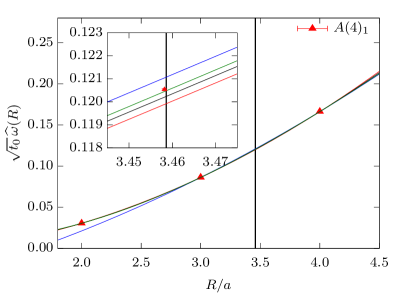
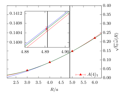
Figure 2: Systematic and statistical errors from the interpolation in $R$ for the ensemble $A(4)_{1}$, which corresponds to the gauge group $\mathrm{SU}(4)$ at a lattice spacing $a\approx 0.1\,\mathrm{fm}$. On the left, for $c=1/2$ , and on the right for $c=1$. In the first case, the statistical error is barely visible in comparison to the systematic one, while in the second case, they are of comparable size.

4 Results

Let us first discuss large $N$ scaling. Before considering the loop observables, we use the scale itself. We can define a second scale similar to $t_{0}$ by changing the numerical pre-factor on the right hand side of Eq. (5). By replacing $0.1125$ with $0.08$ we have a perfectly reasonable scale, which we denote by $t_{0.08}$. As shown on the left panel of Figure 3, choosing the value of $0.08$ we are in the same region where $t^{2}\left\langle E(t)\right\rangle$ grows roughly linearly with $t$ as is the case when $t$ is close to $t_{0}$. Notice that the $N$ dependence is barely visible at the scale of the plot, while on the other hand cut-off effects are large in the region of small $t$.

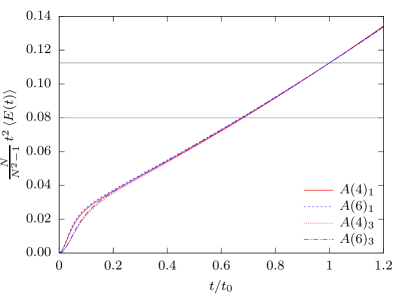
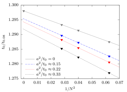
Figure 3: Left: $t^{2}\left\langle E(t)\right\rangle$ as a function of $t$ for several gauge groups and lattice spacings. $A(4)_{1}$ corresponds to an $\mathrm{SU}(4)$ ensemble with $a\approx 0.1\,\mathrm{fm}$, while $A(4)_{3}$ has a lattice spacing $a\approx 0.067\,\mathrm{fm}$. $A(6)_{1}$ and $A(6)_{3}$ correspond to $\mathrm{SU}(6)$ ensembles with the same lattice spacings as the $\mathrm{SU}(4)$ ones correspondingly. Right: large $N$ extrapolations of $t_{0}/t_{0.08}$ at three different lattice spacings and in the continuum. Notice the excellent scaling with $1/N^{2}$ even at this very high accuracy.

On the right panel of Figure 3 we show the large $N$ extrapolations of $t_{0}/t_{0.08}$ and we observe an excellent agreement with a fit to a linear function in $1/N^{2}$. For the three lattice spacings considered, we find the values of $\chi^{2}/\mathrm{dof}$ to be equal to $0.35,\,2.18$ and $1.30$ respectively. In the continuum, the fit is also excellent with a value of $\chi^{2}/\mathrm{dof}=0.96$ and a result for the large $N$ and continuum extrapolation of $t_{0}/t_{0.08}=1.29802(19)$. These results are in complete agreement with the ’t Hooft scaling. They test it with very high accuracies, as the errors in our measurements are $\mathrm{O}(10^{-4})$ (around $10000$ measurements). This allows us to verify the $1/N^{2}$ scaling for this observable even when the finite $N$ corrections are in the percent level.

Let us now turn to the smooth Wilson loop operators. In Figure 4 we show the continuum and large $N$ extrapolations of $W(c=1)$. For the continuum extrapolations, we do a linear fit in $a^{2}/t_{0}$ using only the finer lattices, i.e., those for which $a^{2}/t_{0}<0.25$. With this choice, we take the continuum limit for $\mathrm{SU}(3)$, $\mathrm{SU}(4)$ and $\mathrm{SU}(5)$ using three data points, while we have only two points for $\mathrm{SU}(6)$. To assess the validity of this choice, we also perform a fit including the coarsest data points. We find the two strategies to give compatible extrapolations, so we decide to use the one with fewer points to trade an increase of the statistical error, with the reduction of the systematics due to neglecting higher order terms in the $a$-expansion. The fits are excellent as is displayed on the left panel of Figure 4, and we find similar results for the cases $c=1/2$ and $c=9/4$. Notice that in the case of $\mathrm{SU}(8)$ we have a single point, so we cannot take the continuum limit; hence the right panel in Figure 4 displays the large $N$ extrapolation of the data in the continuum with $N\leq 6$. The large $N$ fit is performed using a quadratic function in $1/N^{2}$, with a value of $\chi^{2}/\mathrm{dof}<0.1$ and a small $1/N^{4}$ coefficient.

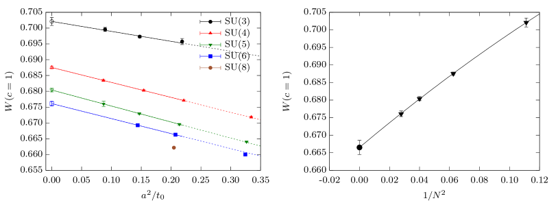
Figure 4: Left: Continuum limit extrapolations of $W(c=1)$. Right: Large $N$ extrapolation of $W(c=1)$ in the continuum. The results are perfectly compatible with a polynomial in $1/N^{2}$ as expected from the ’t Hooft topological expansion.

4.1 Factorization

In order to verify the property of factorization, Eq. (1), we check whether $G_{W}$, Eq. (4), satisfies $G_{W}\to 0$ when $1/N\to 0$. We take the continuum limits for all $N$ except for $N=8$. As before, those lattices for which $a^{2}/t_{0}>0.25$ are used only for validation. We also interpolate to fixed $a^{2}/t_{0}$ given by the one of the $\mathrm{SU}(8)$ ensemble . We can then also use the $\mathrm{SU}(8)$ point for the large $N$ extrapolations at a fixed $a$ ($a^{2}/t_{0}\approx 0.21$). In addition to having an extra point at the larger value of $N=8$, by working at finite lattice spacing, only an interpolation is required for $N<8$, yielding smaller errors. Of course one must keep in mind that the finite $a$ results are not universal; they depend on the regularization, here the Wilson plaquette action. Still, they can be used as a test of large $N$ scaling. Graphs of the large $N$ extrapolations at finite lattice spacing and in the continuum are presented in Figure 5.

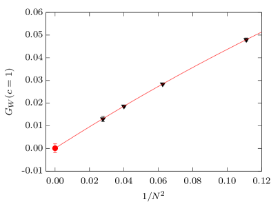
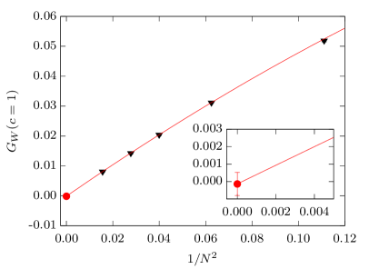
Figure 5: Large $N$ extrapolation of $G_{W}(c=1)$. Left: In the continuum. Right: At finite lattice spacing. In both cases, the fits are done without including the $\mathrm{SU}(3)$ point.

We observe that a quadratic fit excluding $\mathrm{SU}(3)$ correctly extrapolates to $1/N=1/3$ within two, very small, standard deviations at all $c$. While a priori it can’t be expected that the expansion works so well also for $N=3$, this fact serves to increase our confidence in the large $N$ fit. The results of the quadratic fit excluding $\mathrm{SU}(3)$ are presented in Table 1. As shown, the results of the large $N$ extrapolation agree with zero and thus support factorization at all values of $c$. To further validate this conclusion, we perform a fit to the data forcing it to pass through zero when $1/N=0$. The value of $\chi^{2}/\mathrm{dof}$ of the fits can then be used as a criterion to test factorization. For different values of $c$ we present the results for $\chi^{2}/\mathrm{dof}$ at finite lattice spacing of these constrained fits in Table 1. All of them are excellent and support factorization.

Table 1: Results of the large $N$ extrapolations, $\leavevmode\nobreak\ {}^{(1)}$ in the continuum, $\leavevmode\nobreak\ {}^{(2)}$ at finite lattice spacing; and $\leavevmode\nobreak\ {}^{(3)}$, at finite lattice spacing with the constrained fit.

	$c=1/2$	$c=1$	$c=9/4$
$G_{W}(1/N=0)^{(1)}$	$-0.0001(54)$	$-0.0004(73)$	$0.010(13)$
$G_{W}(1/N=0)^{(2)}$	$0.00001(63)$	$-0.0001(6)$	$-0.00074(96)$
$\chi^{2}/\mathrm{dof}^{(2)}$	$<0.01$	$0.01$	$0.18$
$\chi^{2}/\mathrm{dof}^{(3)}$	$<0.01$	$0.03$	$0.38$

So far we have only considered the case $R_{c}=\sqrt{8ct_{0}}$. To study what happens at different values of $R$ we decided to use the loops measured at $c=1/2$ and fix their size such that $\tilde{R}_{c}=2\sqrt{8ct_{0}}$. Let us denote this observable as $G_{\widetilde{W}}$. The analysis is then the same as described earlier except that in this case, when excluding $\mathrm{SU}(3)$ from the fits, the resulting function does not extrapolate to $\mathrm{SU}(3)$. This, however, does not modify the main conclusion, and taking the large $N$ limit shows that factorization also holds. A plot showing our results in the continuum and at finite lattice spacing is displayed in Figure 6.

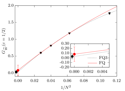
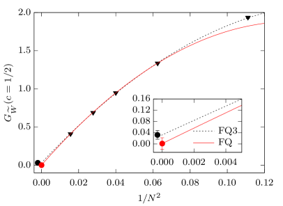
Figure 6: $G_{\widetilde{W}}$ as a function of $N$. On the left in the continuum and on the right at finite lattice spacing. In both cases, we show the fit excluding the $\mathrm{SU}(3)$ point (FQ), and the one including it (FQ3). It is clear that the $\mathrm{O}(1/N^{4})$ corrections are required to include the $\mathrm{SU}(3)$ point and it has to be included in the fit. Both at finite lattice spacing as in the continuum, the large $N$ extrapolation is compatible with factorization.

Finally, we also considered a more complicated observable constructed from the smooth Wilson loops. For that, we define

$$W^{2}_{s}(c)=\frac{a}{(T-2d)}\sum_{x_{0}=d}^{T-d-a}\left(\frac{a^{3}}{L^{3}}\sum_{\vec{x}}W(ct_{0},x_{0},\vec{x},R_{c})\right)^{2}\,,$$ (8)

so that

$$H_{W}(c)=\left(\frac{L^{3}}{t_{0}^{3/2}}\right)\frac{\left\langle W^{2}_{s}(c)\right\rangle-\left\langle W(c)\right\rangle^{2}}{\left\langle W(c)\right\rangle^{2}}\,,$$ (9)

Once again, $H_{W}(c)$ can be used to test factorization, but due to significant finite volume effects for $c\leq 1$, we can only estimate the errors reliably for $c=9/4$. Once more, the results for this observable are compatible with factorization. In this case, we performed a global fit to the data ($\chi^{2}/\mathrm{dof}=1.73$) including the corrections of $\mathrm{O}(1/N^{2})$, $\mathrm{O}(a^{2})$, $\mathrm{O}(a^{2}/N^{2})$ and $\mathrm{O}(1/N^{4})$. The results are shown in Figure 7.

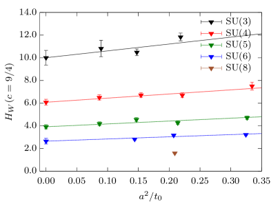
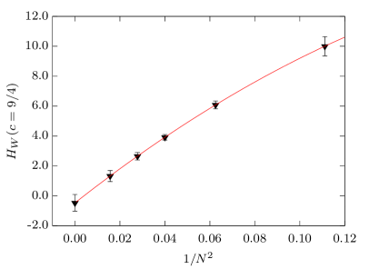
Figure 7: Continuum (left) and large $N$ (right) extrapolations of $H_{W}$ performing a global fit to the data.

5 Conclusions

We have used high precision data to test the scaling in powers of $1/N^{2}$ predicted by the ’t Hooft expansion for the pure gauge theory. By using the gradient flow, we were able to use the smooth Wilson loops and study their $N$ dependence both at finite lattice spacing and in the continuum. In both cases, we have found that the observables are extrapolated to $1/N=0$ in powers of $1/N^{2}$ as expected. Moreover, by using high precision data, we can observe the $N$ dependence at below the percent level. For the observables that we have considered, we find that corrections of $\mathrm{O}(1/N^{2})$ describe very well the data for $N>3$, while including the results at $N=3$ generally requires the addition of a term of $\mathrm{O}(1/N^{4})$.

We have further presented, to our knowledge, the first direct non-perturbative verification of large $N$ factorization for $\mathrm{SU}(N)$ gauge theories on the lattice. While factorization, Eq. (1), holds within our small uncertainties, the corrections at finite $N=3-10$ can be very large, see figs 5,6. Note that $\tilde{G}=1$ or $H=1$ means there is a 100% violation of factorization. These large $1/N^{2}$ corrections are very likely related to the very large $N$ values needed to approach the $1/N=0$ limit in the one-point model GonzalezArroyo:2012fx . In particular, the increase of the $1/N^{2}$ corrections with the size of the loops, which we observe in Figs. 5 and 6, is present in the one-point models Bringoltz:2011by .

Acknowledgements. We would like to thank M. Cè, L. Giusti and S. Schaefer for sharing part of the generation of the gauge configurations Ce:2016awn and M. Koren for useful discussions. Our simulations were performed at the ZIB computer center with the computer resources granted by The North-German Supercomputing Alliance (HLRN). M.G.V acknowledges the support from the Research Training Group GRK1504/2 “Mass, Spectrum, Symmetry” funded by the German Research Foundation (DFG).

References

- (1) G. ’t Hooft, Nucl. Phys. B72, 461 (1974)
- (2) M. Teper, PoS LATTICE2008, 022 (2008), 0812.0085
- (3) B. Lucini, M. Panero, Phys. Rept. 526, 93 (2013), 1210.4997
- (4) L. Del Debbio, H. Panagopoulos, E. Vicari, JHEP 08, 044 (2002), hep-th/0204125
- (5) M. Lüscher, S. Schaefer, JHEP 07, 036 (2011), 1105.4749
- (6) M. CÃ, M. GarcÃa Vera, L. Giusti, S. Schaefer, PoS LATTICE2016, 350 (2016), 1610.08797
- (7) Yu.M. Makeenko, A.A. Migdal, Phys. Lett. 88B, 135 (1979), [Erratum: Phys. Lett.89B,437(1980)]
- (8) L.G. Yaffe, Rev. Mod. Phys. 54, 407 (1982)
- (9) S.R. Coleman, 1/N, in 17th International School of Subnuclear Physics: Pointlike Structures Inside and Outside Hadrons Erice, Italy, July 31-August 10, 1979 (1980), p. 0011, http://www-public.slac.stanford.edu/sciDoc/docMeta.aspx?slacPubNumber=SLAC-PUB-2484
- (10) E. Witten, NATO Sci. Ser. B 59, 403 (1980)
- (11) T. Eguchi, H. Kawai, Phys.Rev.Lett. 48, 1063 (1982)
- (12) A. Gonzalez-Arroyo, M. Okawa, JHEP 07, 043 (2010), 1005.1981
- (13) R. Narayanan, H. Neuberger, JHEP 03, 064 (2006), hep-th/0601210
- (14) M. Lüscher, JHEP 08, 071 (2010), [Erratum: JHEP03,092(2014)], 1006.4518
- (15) M. Lüscher, P. Weisz, JHEP 02, 051 (2011), 1101.0963
- (16) R. Lohmayer, H. Neuberger, JHEP 08, 102 (2012), 1206.4015
- (17) V.S. Dotsenko, S.N. Vergeles, Nucl. Phys. B169, 527 (1980)
- (18) R.A. Brandt, F. Neri, M.a. Sato, Phys. Rev. D24, 879 (1981)
- (19) M. Creutz, Phys. Rev. D23, 1815 (1981)
- (20) M. CÃ, M. GarcÃa Vera, L. Giusti, S. Schaefer, Phys. Lett. B762, 232 (2016), 1607.05939
- (21) M. CÃ, C. Consonni, G.P. Engel, L. Giusti, Phys. Rev. D92, 074502 (2015), 1506.06052
- (22) R. Sommer, Nucl. Phys. B411, 839 (1994), hep-lat/9310022
- (23) A. Gonzalez-Arroyo, M. Okawa, Phys. Lett. B718, 1524 (2013), 1206.0049
- (24) B. Bringoltz, M. Koren, S.R. Sharpe, Phys. Rev. D85, 094504 (2012), 1106.5538