The Boltzmann distribution and the quantum-classical correspondence

Abstract

In this paper we explore the following question: can the probabilities constituting the quantum Boltzmann distribution, $P^{B}_{n}\propto e^{-E_{n}/kT}$, be derived from a requirement that the quantum configuration-space distribution for a system in thermal equilibrium be very similar to the corresponding classical distribution? It is certainly to be expected that the quantum distribution in configuration space will approach the classical distribution as the temperature approaches infinity, and a well-known equation derived from the Boltzmann distribution shows that this is generically the case. Here we ask whether one can reason in the opposite direction, that is, from quantum-classical agreement to the Boltzmann probabilities. For two of the simple examples we consider—a particle in a one-dimensional box and a simple harmonic oscillator—this approach leads to probability distributions that provably approach the Boltzmann probabilities at high temperature, in the sense that the Kullback-Leibler divergence between the distributions approaches zero.

I Introduction

Much has been written about the correspondence between quantum mechanics and classical mechanics. Papers on the subject range from early identifications of similarities, such as the Ehrenfest theorem Ehrenfest and the phase-space representation of quantum mechanics Wigner ; Weyl ; Moyal , to more recent efforts to understand the role of decoherence in the quantum-to-classical transition Zurek ; Schlosshauer ; Halliwell ; Landsman and to assess the status of the correspondence principle in light of chaotic dynamics Landsman ; Ikeda ; Belot . In this paper we study a specific aspect of the quantum-classical correspondence, namely, the way in which the quantum mechanical configuration-space distribution for a system in thermal equilibrium approaches its classical counterpart as the temperature gets large. (The questions we raise here could also be raised for probability distributions over other slices of phase space. But in this paper we restrict our attention to the configuration-space distribution.)

For each of the examples we consider here, which are all quite simple and in fact involve only a one-dimensional configuration space, we observe that the quantum distribution becomes quite similar to the classical distribution even at modest values of the temperature. This similarity depends on a kind of coordination between the shapes of the quantum mechanical energy eigenfunctions (in the position representation) and the Boltzmann weights with which the squares of these eigenfunctions are averaged in a thermal mixture: these two elements work together to produce a high level of agreement with the classical distribution. The degree of this agreement leads us to ask whether the probabilities constituting the quantum Boltzmann distribution, $P^{B}_{n}\propto e^{-E_{n}/kT}$ (which together with the energy eigenstates define the canonical ensemble), can be deduced from a requirement that the quantum position distribution be very similar to the classical position distribution. If such a deduction is indeed possible, it may indicate a tighter network of connections among quantum mechanics, classical mechanics, and statistical mechanics than we normally recognize. After all, we already have other, apparently independent ways of deriving the Boltzmann distribution.

We do not answer our question in general—it seems to be a difficult one. Rather, we show how a derivation of the Boltzmann probabilities can be achieved in our examples, at least for high temperatures, and we argue that the matter is worth further investigation. Crucially, in trying to arrive at the probabilities $P^{B}_{n}$, we do not put into the mathematics the energy eigenvalues $E_{n}$ but only the squares of the energy eigenfunctions.

To be sure, one expects the quantum distribution in configuration space to approach the corresponding classical distribution as the temperature gets large. One way to see this is through the following well-known approximate expression for the quantum distribution (based on the Boltzmann formula), in which only those terms up to second order in $\hbar$ have been kept Oppenheim (the approximation is written here for the one-dimensional case):

$$\begin{split}\rho_{q}(x)\propto&\left\{1+\hbar^{2}\left[\left(-\frac{1}{12mk^{2}T^{2}}\right)\frac{d^{2}V(x)}{dx^{2}}\right.\right.\\ &\left.\left.+\,\frac{1}{24mk^{3}T^{3}}\left(\frac{dV(x)}{dx}\right)^{2}\right]\right\}e^{-V(x)/kT}.\end{split}$$ (1)

Here $V(x)$ is the potential energy and $m$ is the particle’s mass. As the classical position distribution $\rho_{c}(x)$ is simply proportional to $e^{-V(x)/kT}$, Eq. (1) predicts that as the temperature approaches infinity, the ratio $\rho_{q}(x)/\rho_{c}(x)$ approaches the constant value 1. We could use Eq. (1) or related equations to try to account for the similarity we see between the quantum and classical cases fn1 , but our aim in this paper is not so much to account for this similarity as to use it as a starting point for generating the Boltzmann probabilities.

In the following sections we consider three simple examples, again all in one spatial dimension: (i) a particle in a box with infinitely hard walls, (ii) a harmonic oscillator, and (iii) a particle in a linear potential bounded by a hard wall. For each example, we begin by illustrating the similarity between the quantum and classical position distributions. Then we ask this question: given the classical position distribution and the squares of the quantum energy eigenfunctions, how should the latter be weighted in order to produce a position distribution “as close as possible” to the classical one? Or, slightly more precisely, if we let $\rho(x)$ be the position distribution resulting from the weighting of the squared eigenfunctions, we ask how the weights should be chosen so as to make the ratio $r(x)=\rho(x)/\rho_{c}(x)$ “as flat as possible,” where $\rho_{c}(x)$ is the classical thermal distribution at some temperature $T$. We particularly want to know whether the optimal weighting is similar to the Boltzmann weighting, and whether it approaches the Boltzmann weighting as the temperature gets large newfootnote .

Ideally we would adopt a single, simple interpretation of “as flat as possible” that applies to all our examples, but we have not found such an interpretation that is mathematically tractable. Instead, in each case we interpret “as flat as possible” in a way that makes the mathematics manageable for that example. These ad hoc interpretations are, however, sufficiently similar to each other that they can guide us, in Section V, to a general definition of “as flat as possible” that we can reasonably hope will generate the Boltzmann probabilities, in the high-temperature limit, for a large class of systems.

The final section then discusses the potential significance of our observations.

II Particle in a box

Consider a one-dimensional particle of mass $m$ confined to a box with hard walls at the positions $x=0$ and $x=L$. The quantum energy eigenvalues for this system are $E_{n}=\pi^{2}\hbar^{2}n^{2}/(2mL^{2})$, where $n=1,2,\ldots$. In terms of a rescaled position $\xi=x/L$ and a rescaled temperature $\tau=kT/E_{1}$, the energy eigenfunctions are

$$\psi_{n}(\xi)=\sqrt{2}\sin(\pi n\xi),\hskip 5.69054ptn=1,2,\ldots,$$ (2)

and the Boltzmann probabilities with which these eigenfunctions are weighted in thermal equilibrium are

$$P^{B}_{n}=\frac{1}{Z}e^{-n^{2}/\tau},$$ (3)

where $Z=\sum_{n=1}^{\infty}e^{-n^{2}/\tau}$. Thus, in thermal equilibrium, the quantum distribution of the particle’s position is

$$\begin{split}\rho_{q}(\xi)&=\sum_{n=1}^{\infty}P^{B}_{n}|\psi_{n}(\xi)|^{2}=1-\sum_{n=1}^{\infty}P^{B}_{n}\cos(2\pi n\xi)\\ &=\frac{\theta_{3}(0,e^{-1/\tau})-\theta_{3}(\pi\xi,e^{-1/\tau})}{\theta_{3}(0,e^{-1/\tau})-1},\end{split}$$ (4)

where $\theta_{3}$ is the Jacobi theta function $\theta_{3}(z,q)=\sum_{n=-\infty}^{\infty}q^{n^{2}}e^{2niz}$. Meanwhile the analogous classical distribution of the particle’s position, at any non-zero temperature, is simply the uniform distribution (because inside the box, the potential energy does not depend on position):

$$\rho_{c}(\xi)=1.$$ (5)

Fig. 1 plots the quantum position distribution $\rho_{q}(\xi)$ for the temperature $\tau=60$. This is not a particularly high temperature: the first fourteen energy eigenstates carry 99% of the probability. And yet the distribution is already quite flat. We write down here the values of $\rho_{q}(\xi)$ at $\xi=0.2$ and $\xi=0.5$:

$$\begin{split}\rho_{q}(0.2)=1.07855849250\\ \rho_{q}(0.5)=1.07855849256\end{split}$$ (6)

Moreover, one can show, from known properties of the Jacobi theta function, that the function $\rho_{q}(\xi)$ is monotonically increasing between $\xi=0$ and $\xi=1/2$ (and of course it is symmetric around $\xi=1/2$). Thus it seems that the Boltzmann probabilities in Eq. (3) weight the sinusoidal functions $|\psi_{n}(\xi)|^{2}$ in just the right way as to produce a distribution that, over most of the interval, is almost as flat as the corresponding classical distribution.

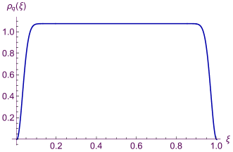
Figure 1: The thermal position distribution of a quantum particle in a box. Here $kT=60E_{1}.$

We now ask whether one can deduce the Boltzmann weights from a requirement that the position distribution be very flat. To address this question, we consider a general weighting of the squared energy eigenfunctions:

$$\rho(\xi)=\sum_{n=1}^{\infty}P_{n}|\psi_{n}(\xi)|^{2},$$ (7)

where the probabilities $P_{n}$ are to be determined. We could ask what values of $P_{n}$ make $\rho(\xi)$ as flat as possible. But it is clear that this is not the right question: making the distribution as flat as possible is like taking the infinite-temperature limit, which is not what we want. (The quantum distribution becomes completely flat at infinite temperature, but in that limit every $P_{n}$ approaches zero.) Rather, we want somehow to limit the effective temperature so that we can compare the $P_{n}$’s that emerge from a flatness condition to the $P^{B}_{n}$’s given by the Boltzmann distribution.

Here we take a fairly crude approach to limiting the effective temperature: we simply restrict the sum in Eq. (7) to the first $N$ eigenstates.

$$\rho(\xi)=\sum_{n=1}^{N}P_{n}|\psi_{n}(\xi)|^{2}.$$ (8)

Now we take as our flatness condition the requirement that the first $2N-1$ derivatives of $\rho(\xi)$, evaluated at $\xi=1/2$ (that is, at the middle of the box), be zero. We have chosen the number $2N-1$ so that the number of conditions we are imposing equals the number of variables. The odd-numbered derivatives are automatically zero at $\xi=1/2$ because of the symmetry of the functions $|\psi_{n}(\xi)|^{2}$. Thus our flatness condition, together with the normalization condition, yields exactly $N$ linear equations for the $N$ variables $P_{n}$. Upon taking the derivatives, one finds that the equations are

$$\begin{split}&\sum_{n=1}^{N}(-1)^{n}n^{2m}P_{n}=0,\hskip 28.45274ptm=1,2,\ldots,N-1\\ &\sum_{n=1}^{N}P_{n}=1.\end{split}$$ (9)

This system of linear equations can be solved exactly. The unique solution (see Appendix A) is

$$P_{n}=A\frac{(2N)!}{(N+n)!(N-n)!},$$ (10)

where the proportionality constant $A$ is determined by normalization. This constant comes out to be

$$A=2\left[2^{2N}-\frac{(2N)!}{N!^{2}}\right]^{-1}.$$ (11)

Thus the position distribution $\rho(\xi)$ is made optimally flat, in our sense, by choosing the $P_{n}$’s to form essentially half of a binomial distribution.

Now, the Boltzmann formula for a particle in a box, Eq. (3), has the form of a discrete Gaussian function of $n$. We know that a binomial distribution ultimately approaches a Gaussian, so we expect our binomial “flatness-optimizing” distribution to look much like the Boltzmann distribution when $N$ is large, as long as we make a judicious choice of the correspondence between the temperature $\tau$ (for the Boltzmann distribution) and the value of $N$ (for the flatness-optimizing distribution). It turns out that the choice $\tau=N$ works well. Fig. 2 shows the two probability distributions for $\tau=N=7$. As the temperature increases, the flatness-optimizing distribution $\{P_{n}\}$ approaches the Boltzmann distribution $\{P^{B}_{n}\}$ in the sense that the Kullback-Leibler divergence,

$$D(P|P^{B})=\sum_{n=1}^{N}P_{n}\ln\left(P_{n}/P^{B}_{n}\right),$$ (12)

approaches zero, as illustrated in Fig. 3. One can in fact show analytically (Appendix B) that this divergence diminishes as $1/N^{2}$ for large $N$. Thus although our flatness-optimizing distribution is not identical to the Boltzmann distribution—it could not be, since it is limited to the first $N$ eigenstates—it approaches the Boltzmann distribution in a rather strong sense as the temperature increases. We regard this asymptotic result as interesting, because it seems so different from the usual way of deriving these probabilities.

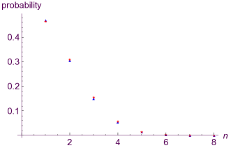
Figure 2: The Boltzmann probabilities (blue triangles) and the probabilities that make $\rho(\xi)$ optimally flat (red stars). In this plot $\tau=N=7$. For much larger values of $\tau$, it is difficult to see any difference between the two distributions in a plot like this.

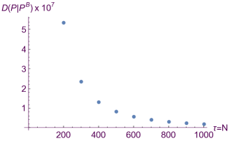
Figure 3: The Kullback-Leibler divergence $D(P|P^{B})$ between the flatness-optimizing distribution $\{P_{n}\}$ and the Boltzmann distribution $\{P^{B}_{n}\}$. To make the comparison, we have set the value of $N$ in $P_{n}$ equal to the value of $\tau$ in $P^{B}_{n}$.

Regarding the infinite-temperature limit, we note that merely requiring the position distribution $\rho(\xi)$ to become flat in this limit is not enough to see anything special about the Boltzmann probabilities $P^{B}_{n}$. Consider, for example, the alternative set of probabilities $P^{A}_{n}=$ $(e^{1/\tau}-1)e^{-n/\tau}$. (The “A” is for “alternative.”) The resulting position distribution,

$$\rho^{A}(\xi)=\sum_{n=1}^{\infty}P^{A}_{n}|\psi_{n}(\xi)|^{2}=\frac{(e^{1/\tau}+1)(1-\cos(2\pi\xi))}{e^{1/\tau}-2\cos(2\pi\xi)+e^{-1/\tau}}\;\,,$$ (13)

likewise becomes arbitrarily flat as $\tau$ goes to infinity. But $P^{A}_{n}$ is clearly very different from $P^{B}_{n}$. Evidently one needs some kind of finite-temperature flatness condition in order to arrive at something that approaches the Boltzmann distribution in the infinite-temperature limit.

Again we emphasize that, in our flatness-optimizing problem, we have not put into the mathematics the energy eigenvalues. (We have put into the mathematics the squared eigenfunctions $|\psi_{n}(\xi)|^{2}$, together with an ordering of these eigenfunctions, but we have not explicitly put in the associated energies.) So, to the extent that the Boltzmann formula emerges from the flatness condition, part of what emerges is the fact that the exponent in this formula is proportional to $n^{2}$.

Our insistence on flatness of the position distribution may bring to mind Jaynes’ characterization of the thermal state as the state of maximum entropy for a fixed value of the average energy Jaynes . Perhaps even more relevant is the recent work by Anzà and Vedral on states for which the Shannon entropy of a particular observable is maximized for fixed average energy Anza . One might suppose from the above results that, for the particle in a box, the position is an observable whose differential entropy $h=-\int_{0}^{1}\rho(\xi)\ln\rho(\xi)d\xi$ is maximized in the thermal state; that is, one might imagine that the observed flatness of the function $\rho(\xi)$ is a manifestation of position-entropy maximization. However, it turns out that this is not the case, at least not if the average energy is being held fixed. It is easy to find states with the same average energy as the thermal state but exhibiting a greater position-entropy.

Of course, in our problem we did not hold the average energy fixed. Rather, we fixed the value of $N$, which labels the highest-energy eigenstate allowed to have nonzero probability. But if one tries maximizing the position-entropy $h$ while holding $N$ fixed, one finds that the result is quite different from the Boltzmann distribution. So, if there is a connection between our observations and Jaynes’ principle, it must be a subtler connection.

III Harmonic oscillator

Consider a one-dimensional harmonic oscillator in thermal equilibrium. The potential energy function is $V(x)=(1/2)m\omega^{2}x^{2}$, where $m$ is the mass and $\omega$ is the angular frequency. In terms of a rescaled position variable $\xi=x\sqrt{m\omega/\hbar}$ and a rescaled temperature $\tau=kT/(\hbar\omega)$, the squared energy eigenfunctions are

$$|\psi_{n}(\xi)|^{2}=\frac{1}{2^{n}n!\sqrt{\pi}}e^{-\xi^{2}}H^{2}_{n}(\xi),\hskip 8.53581ptn=0,1,\ldots,$$ (14)

and the Boltzmann probabilities are

$$P^{B}_{n}=(1-e^{-1/\tau})e^{-n/\tau}.$$ (15)

In Eq. (14), $H_{n}(\xi)$ is the Hermite polynomial

$$H_{n}(\xi)=(-1)^{n}e^{\xi^{2}}\frac{d^{n}}{d\xi^{n}}e^{-\xi^{2}}.$$ (16)

The quantum mechanical thermal position distribution is therefore

$$\begin{split}\rho_{q}(\xi)&=\sum_{n=0}^{\infty}P^{B}_{n}|\psi_{n}(\xi)|^{2}\\ &=\frac{1}{\sqrt{\pi}}(1-e^{-1/\tau})e^{-\xi^{2}}\sum_{n=0}^{\infty}\frac{e^{-n/\tau}}{2^{n}n!}H^{2}_{n}(\xi).\end{split}$$ (17)

It is well known that the sum in Eq. (17) comes out to be an exact Gaussian. The distribution $\rho_{q}(\xi)$ can be rewritten as Hillery

$$\rho_{q}(\xi)=\frac{1}{\sqrt{2\pi\langle\xi^{2}\rangle}}e^{-\frac{\xi^{2}}{2\langle\xi^{2}\rangle}},$$ (18)

where

$$\langle\xi^{2}\rangle=\frac{1}{2\tanh(\frac{1}{2\tau})}.$$ (19)

Meanwhile the classical position distribution, proportional to $e^{-V(x)/kT}$, when written in terms of our rescaled variables becomes

$$\rho_{c}(\xi)=\frac{1}{\sqrt{2\pi\tau}}e^{-\frac{\xi^{2}}{2\tau}}.$$ (20)

From Eqs. (18) and (20) it is clear that $\rho_{q}$ differs from $\rho_{c}$ only because $\langle\xi^{2}\rangle$ is not the same as $\tau$ (reflecting the quantum violation of the classical equipartition theorem).

In the preceding section, we asked what probability distribution $\{P_{n}\}$ would make the quantum position distribution for the particle in a box as flat as possible (in a certain sense), so that it would be as close as possible to the uniform classical distribution. We found that the resulting probability distribution $\{P_{n}\}$, while not equal to the Boltzmann distribution $\{P^{B}_{n}\}$, did approach that distribution in the high-temperature limit. We can ask a similar question here. Given the classical position distribution $\rho_{c}(\xi)$ for a given value of $\tau$, and given the squared energy eigenstates $|\psi_{n}(\xi)|^{2}$ of the harmonic oscillator, we ask how the probabilities $P_{n}$ should be chosen so that the weighted average,

$$\rho(\xi)=\sum_{n=0}^{\infty}P_{n}|\psi_{n}(\xi)|^{2},$$ (21)

makes the ratio $r(\xi)=\rho(\xi)/\rho_{c}(\xi)$ as flat as possible. Do the optimal probabilities $P_{n}$ look like the Boltzmann probabilities given in Eq. (15), and do they approach those probabilities at high temperature?

In this case we can take “as flat as possible” to mean “exactly constant”: as long as $\tau$ is at least 1/2, we can simply choose the $P_{n}$’s to be the quantum probabilities evaluated at whatever temperature is required to make the spread of the quantum Gaussian equal to that of the classical Gaussian. Then $\rho(\xi)$ of Eq. (21) will be exactly equal to the classical distribution $\rho_{c}(\xi)$. (If $\tau$ is less than 1/2, the classical spread is less than the spread of the quantum ground state. A quantum particle cannot achieve such a narrow distribution.) Specifically, we choose $P_{n}$ to be

$$P_{n}=(1-e^{-1/\tau_{e}})e^{-n/\tau_{e}},$$ (22)

where the effective temperature $\tau_{e}$ is given by

$$\frac{1}{2\tau_{e}}=\tanh^{-1}\left(\frac{1}{2\tau}\right).$$ (23)

That is, $\tau_{e}$ is the value we have to substitute for the $\tau$ in Eq. (19) in order to make $\langle\xi^{2}\rangle$—the quantum variance—equal to the actual value of $\tau$, which is the classical variance. Equations (22) and (23) define our optimal $P_{n}$’s for the given value of $\tau$. (The latter equation makes clear that we cannot achieve equality with the classical distribution if $\tau$ is less than 1/2.)

As we did in the preceding section, we again ask whether the probabilities $P_{n}$ that make the weighted average closest to the classical distribution approach the Boltzmann distribution $P^{B}_{n}$ in the Kullback-Leibler sense as the temperature approaches infinity. In this case the Kullback-Leibler divergence can be worked out exactly. One finds that

$$D(P|P^{B})=\log\left(\frac{1-e^{-1/\tau_{e}}}{1-e^{-1/\tau}}\right)+\frac{e^{-1/\tau_{e}}}{1-e^{-1/\tau_{e}}}\left(\frac{1}{\tau}-\frac{1}{\tau_{e}}\right).$$ (24)

Expanding this function out in powers of $1/\tau$ (using Eq. (23)), we get that

$$D(P|P^{B})=\frac{1}{288}\cdot\frac{1}{\tau^{4}}+\,{\mathcal{O}}\left(\frac{1}{\tau^{6}}\right).$$ (25)

So the “classical-mimicking” distribution $\{P_{n}\}$ does approach the Boltzmann distribution rapidly.

In a certain sense, our results for the harmonic oscillator are not as impressive as for the particle in a box. In order to get our “classical-mimicking” probabilities for the harmonic oscillator, we needed to invoke, at the outset, the classical Boltzmann factor $e^{-V(x)/kT}$. Thus it may not be terribly surprising that the quantum Boltzmann factor, $e^{-E_{n}/kT}$, emerged from the calculation (asymptotically). (In Section VI, we ask whether what we have seen in this example points to a special property of the exponential form of the Boltzmann factor.) Still, though, there is the notable fact that we did not put the energy eigenvalues into our calculation. They are part of what emerges.

IV Particle in a linear potential

We now consider a case that combines features of both of the previous examples: a hard wall and an otherwise continuously varying potential. For a particle of mass $m$ in one dimension, let the potential energy function be $V(x)=\alpha x$ for $x\geq 0$, with a hard wall at $x=0$. We use the rescaled position and temperature variables

$$\xi=x\left(\frac{2m\alpha}{\hbar^{2}}\right)^{1/3}\hskip 28.45274pt\tau=kT\left(\frac{2m}{\hbar^{2}\alpha^{2}}\right)^{1/3}.$$ (26)

Then the squared energy eigenfunctions are (for $\xi\geq 0$)

$$|\psi_{n}(\xi)|^{2}=\frac{\operatorname{Ai}(\xi+u_{n})^{2}}{\operatorname{Ai}^{\prime}(u_{n})^{2}}.$$ (27)

Here $\operatorname{Ai}$ is the Airy function, $\operatorname{Ai}^{\prime}$ is its derivative, and $u_{n}$ is the $n$th zero of the Airy function (all the $u_{n}$’s are negative). The Boltzmann probabilities with which the $|\psi_{n}|^{2}$’s are weighted in thermal equilibrium are

$$P^{B}_{n}=\frac{1}{Z}e^{u_{n}/\tau},$$ (28)

where $Z=\sum_{n=1}^{\infty}e^{u_{n}/\tau}$. So the quantum mechanical position distribution is

$$\rho_{q}(\xi)=\sum_{n=1}^{\infty}P^{B}_{n}|\psi_{n}(\xi)|^{2}=\frac{1}{Z}\sum_{n=1}^{\infty}\frac{e^{u_{n}/\tau}\operatorname{Ai}(\xi+u_{n})^{2}}{\operatorname{Ai}^{\prime}(u_{n})^{2}}$$ (29)

The classical position distribution is simply

$$\rho_{c}(\xi)=(1/\tau)e^{-\xi/\tau}.$$ (30)

Fig. 4 shows both of these position distributions for $\tau=2$, and Fig. 5 shows the ratio $r(\xi)=\rho_{q}(\xi)/\rho_{c}(\xi)$. At this relatively low value of the temperature, the two distributions are notably different, but the ratio is remarkably uniform beyond a narrow boundary region near the wall. For $\xi>6$, the ratio appears to be constant to 30 decimal places (though not exactly constant). Fig. 6 shows the contributions to the ratio $r(\xi)$ from the first four energy eigenfunctions. Note that the Boltzmann weights seem to give these contributions precisely the right height so that they sum to an almost constant function (except close to the wall).

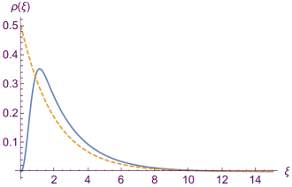
Figure 4: The quantum (solid blue) and classical (dashed gold) position distributions for a particle in a linear potential with a hard wall at $\xi=0$. Here $\tau=2$.

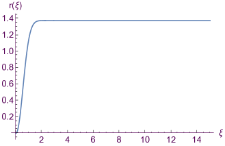
Figure 5: The ratio $r(\xi)=\rho_{q}(\xi)/\rho_{c}(\xi)$ for $\tau=2$. Beyond $\xi=6$, this ratio appears to be constant to 30 decimal places (though not exactly constant).

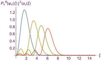
Figure 6: The first four squared energy eigenfunctions for the linear potential, each weighted by the appropriate Boltzmann weight $P^{B}_{n}$ and divided by $\rho_{c}(\xi)$. The sum of these curves and their successors yields the function $r(\xi)$ of Fig. 5.

For this example, we have not been able to formulate a sharp and tractable optimization problem that would define a set of $P_{n}$’s making the ratio

$$r(\xi)=\frac{\rho(\xi)}{\rho_{c}(\xi)}=\frac{\sum_{n=1}^{\infty}P_{n}|\psi_{n}(\xi)|^{2}}{\rho_{c}(\xi)}$$ (31)

“as flat as possible.” (But see Section V, in which we propose one reasonable formulation of the problem, though not a formulation that we have been able to solve.) It is nevertheless possible to interpret “as flat as possible” in a weaker sense, which does at least seem to pick out the Boltzmann values $P^{B}_{n}$ for large values of $n$. We can see this through the following informal argument.

We begin by writing $r(\xi)$ explicitly in terms of the Airy function:

$$r(\xi)=\tau e^{\xi/\tau}\sum_{n=1}^{\infty}P_{n}\frac{\operatorname{Ai}(\xi+u_{n})^{2}}{\operatorname{Ai}^{\prime}(u_{n})^{2}}.$$ (32)

Let us now define $R_{n}$ by

$$P_{n}=\operatorname{Ai}^{\prime}(u_{n})^{2}e^{u_{n}/\tau}R_{n}.$$ (33)

In terms of $R_{n}$, we have

$$r(\xi)=\tau\sum_{n=1}^{\infty}R_{n}f(\xi+u_{n}),$$ (34)

where $f(z)=e^{z/\tau}\operatorname{Ai}(z)^{2}$. That is, $r(\xi)$ (for $\xi\geq 0$) is a weighted sum of an infinite number of shifted versions of the same function $f(z)$.

Now, if $r(\xi)$ is to be almost constant for large $\xi$, in particular we must have that, for large $s$ and $t$ with $t>s$,

$$\int_{|u_{s}|}^{|u_{t}|}r(\xi)d\xi\approx A(\tau)(|u_{t}|-|u_{s}|),$$ (35)

where $A(\tau)$ is independent of $s$ and $t$. We now substitute the expression in Eq. (34) for the $r(\xi)$ in this integral. Our condition for flatness becomes

$$\tau\sum_{n=1}^{\infty}R_{n}\int_{|u_{s}|}^{|u_{t}|}f(\xi+u_{n})d\xi\approx A(\tau)(|u_{t}|-|u_{s}|).$$ (36)

The function $f(z)$ has a characteristic width that depends on the value of $\tau$. (If we normalize $f(z)$ so as to turn it into a probability distribution, we find that the width of $f(z)$, quantified by the standard deviation $\Updelta z$, is approximately equal to $\tau/\sqrt{2}$ for large $\tau$.) Let us now consider the special case where both $|u_{t}|-|u_{s}|$ and $|u_{s}|$ are much larger than this characteristic width. Then for most of those terms in the sum in Eq. (36) for which $s<n<t$, the range of integration completely spans the region where the integrand is significantly different from zero, and we can write

$$\int_{|u_{s}|}^{|u_{t}|}f(\xi+u_{n})d\xi\approx\int_{-\infty}^{\infty}f(z)dz=\frac{\sqrt{\tau}}{2\sqrt{\pi}}e^{1/(12\tau^{3})}.$$ (37)

Meanwhile, for most of those terms for which $n$ is outside of the range $s<n<t$, the integral is approximately zero. We can therefore further approximate our condition for flatness (Eq. (36)) to be

$$\sum_{n=s}^{t}R_{n}\approx B(\tau)(|u_{t}|-|u_{s}|),$$ (38)

where $B(\tau)$ is another function of $\tau$ that does not depend on $s$ and $t$. For Eq. (38) to be true regardless of the values of $s$ and $t$, we want $R_{n}$ to have the form

$$R_{n}\approx B(\tau)(|u_{n}|-|u_{n-1}|).$$ (39)

(Or we could say, $R_{n}\approx B(\tau)(|u_{n+1}|-|u_{n}|)$. At this level of approximation, the two expressions are equivalent.) It is known that $|u_{n}|-|u_{n-1}|$ is roughly proportional to $n^{-1/3}$ for large $n$ NIST . So we want $R_{n}$ to be roughly proportional to $n^{-1/3}$, and, according to Eq. (33), we therefore want $P_{n}$ to satisfy

$$P_{n}\propto n^{-1/3}\operatorname{Ai}^{\prime}(u_{n})^{2}e^{u_{n}/\tau}.$$ (40)

Finally, it is also known that for large $n$, the combination $n^{-1/3}\operatorname{Ai}^{\prime}(u_{n})^{2}$ is nearly constant. (The limiting value for infinite $n$ is $(3/(2\pi^{2}))^{1/3}$ NIST .) We therefore arrive at

$$P_{n}\propto e^{u_{n}/\tau},$$ (41)

where we expect the proportionality constant to depend on the temperature. But Eq. (41) agrees with the form of the Boltzmann probabilities (Eq. (28)). In this way we can see how, at least for large $n$, the Boltzmann probabilities $P^{B}_{n}\propto e^{u_{n}/\tau}$ naturally arise if one is trying to make the ratio $r(\xi)$ roughly constant.

Note that, as in the earlier sections, our argument is based only on the squared energy eigenfunctions $|\psi_{n}(\xi)|^{2}$ and not the associated energies. (We may not be able to write down those eigenfunctions without knowing the energies, but conceptually it is still the squared eigenfunctions and not the energies that enter the argument.)

V A general definition of “as flat as possible”?

The main problem we have considered is this: Given the squares of the energy eigenfunctions in the position representation, how can these eigenfunctions be weighted so as to yield a function $\rho(x)$ for which $\rho(x)/\rho_{c}(x)$ is “as flat as possible”? (Again, $\rho_{c}(x)$ is the classical thermal position distribution at a given temperature.) In the first two examples (the particle in a box and the harmonic oscillator), the probability distributions generated in this way turned out to approach, in the Kullback-Leibler sense, the quantum Boltzmann distribution in the limit of infinite temperature. The third example (the particle in a linear potential) also seemed to produce something like the Boltzmann distribution, though our argument in that case is not rigorous.

But so far we have interpreted “as flat as possible” in an ad hoc way. It is interesting to ask whether one can come up with a general definition of “as flat as possible” that would yield the Boltzmann probabilities, in this asymptotic sense, for a large class of systems. Our results for the three examples we have considered in this paper suggest that the following approach might work.

For now let us restrict ourselves to the one-dimensional case. Let the position $x$ run from $a$ to $b$, where $a$ might be $-\infty$ and $b$ might be $\infty$. Given the classical position distribution $\rho_{c}(x)$ associated with a given temperature, let us begin by defining a new variable $y$ by

$$y=\int_{a}^{x}\rho_{c}(x^{\prime})dx^{\prime}.$$ (42)

Then $y$ runs from $0$ to $1$ (since $\rho_{c}$ is normalized), and the classical distribution for $y$ is the uniform distribution (just as it is for $\xi$ in the case of the particle in a box). We now consider, for each energy eigenstate $\psi_{n}(x)$, the corresponding distribution of the variable $y$—let us call it $\sigma_{n}(y)$—so that a weighted average of these $\sigma_{n}(y)$’s would yield some overall distribution $\sigma(y)$. We want $\sigma(y)$ to be “as flat as possible.” Before we write down our proposed definition of “as flat as possible,” let us illustrate the construction of $\sigma(y)$ by considering the example of the linear potential.

Recall that for the linear potential, in terms of the dimensionless variable $\xi$, we have

$$\rho_{c}(\xi)=(1/\tau)e^{-\xi/\tau}.$$ (43)

So

$$y=\int_{0}^{\xi}\rho_{c}(\xi^{\prime})d\xi^{\prime}=1-e^{-\xi/\tau}.$$ (44)

Let $\rho_{n}(\xi)=|\psi_{n}(\xi)|^{2}=\operatorname{Ai}(\xi+u_{n})^{2}/\operatorname{Ai}^{\prime}(u_{n})^{2}$ be the $n$th squared eigenfunction. The corresponding distribution $\sigma_{n}(y)$ is defined by

$$\sigma_{n}(y)dy=\rho_{n}(\xi)d\xi.$$ (45)

So in this example,

$$\sigma_{n}(y)=\rho_{n}(\xi)\frac{d\xi}{dy}=\left(\frac{\tau}{1-y}\right)\frac{\operatorname{Ai}[-\tau\ln(1-y)+u_{n}]^{2}}{\operatorname{Ai}^{\prime}(u_{n})^{2}}.$$ (46)

A general weighted average would be

$$\sigma(y)=\sum_{n=1}^{\infty}P_{n}\sigma_{n}(y).$$ (47)

For the special case where the $P_{n}$’s are the Boltzmann weights $P_{n}^{B}\propto e^{u_{n}/\tau}$, for $\tau=2$ we get the curve $\sigma_{q}(y)$ shown in Fig. 7.

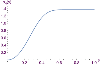
Figure 7: The quantum position distribution for a particle in a linear potential when position is parameterized by the variable $y$. Here $\tau=2$.

We now present our proposed definition of “as flat as possible.” For any small $\epsilon$ greater than zero, let $Y_{\epsilon}$ be the set of all values of $y$ for which $\sigma(y)\geq\sigma_{max}-\epsilon$, where $\sigma_{max}$ is the maximum value of $\sigma(y)$, if the maximum exists. (For the harmonic oscillator with $\tau<1/2$, the function $\sigma(y)$ will take arbitrarily large values no matter how the eigenstates are weighted, because each $\sigma_{n}(y)$ itself takes arbitrarily large values. So our definition will not apply to that case.) For each value of $\epsilon$, we can look for a distribution $\{P^{\epsilon}_{n}\}$ that maximizes the measure of the set $Y_{\epsilon}$ (for the standard measure on the interval $[0,1]$). (For an exceptional case such as the particle in a box, in which the classical position distribution is independent of temperature, we need to limit the effective temperature in some way in order to get a solution, as we did in Section II.) We can then define our optimal distribution $\{P_{n}\}$ to be the limit of $\{P^{\epsilon}_{n}\}$ as $\epsilon$ approaches zero, if the limit exists. This formulation of the problem is consistent with our definition of “as flat as possible” for the harmonic oscillator (for $\tau\geq 1/2$). It is also plausibly consistent with what we did for the particle in a box: if the sole maximum of $r(\xi)$ occurs at the center of the box, then one wants the derivatives of as many orders as possible to be zero at the center in order to make $r(\xi)$ as constant as possible near that location. For the third example, we have nothing rigorous to report, but this general formulation seems sensible for that case as well.

We can express this same proposed definition in terms of the original variable $x$. For any small $\epsilon$ greater than zero, let $X_{\epsilon}$ be the set of all values of $x$ for which $r(x)\geq r_{max}-\epsilon$, where, as usual, $r(x)=\rho(x)/\rho_{c}(x)$ and $\rho(x)=\sum_{n}P_{n}|\psi_{n}(x)|^{2}$. Here $r_{max}$ is the supremum of $r(x)$ over the range of $x$ (if the supremum exists). Now we look for a distribution $\{P^{\epsilon}_{n}\}$ for which the probability of the set $X_{\epsilon}$ is greatest, where the probability is computed using the classical thermal distribution $\rho_{c}(x)$. That is, the probability we want to maximize is

$$\hbox{probability of $X_{\epsilon}$}\;=\int_{x\in X_{\epsilon}}\rho_{c}(x)dx.$$ (48)

We then take the limit of $\{P^{\epsilon}_{n}\}$ as $\epsilon$ goes to zero.

In a higher-dimensional configuration space, there is an obvious generalization of the above criterion. In fact, the preceding paragraph can simply be reinterpreted, with $x$ referring to the location in a multidimensional space.

We also need to consider the possibility of a degeneracy in energy. Within a degenerate subspace, there is no unique set of squared energy eigenfunctions, since one has a choice of basis for the subspace. In that case, we can simply use, for each degenerate subspace, the configuration-space distribution associated with the completely mixed state over that subspace. The question would then be how to weight the distributions associated with distinct energies so as to make $r(x)$ as flat as possible.

Now, there certainly exist systems for which our approach does not work. A simple example is a particle on a one-dimensional ring (that is, a one-dimensional box with periodic boundary conditions). In that case every energy eigensubspace is associated with a uniform position distribution. So the quantum position distribution automatically agrees with the classical position distribution regardless of how these subspaces are weighted relative to each other. Moreover, it is not clear that using the other dimension of phase space would help in this case: in the quantum case the momentum does not even take the same set of values as in the classical case. Perhaps it should not be surprising if our approach, based largely on a comparison between classical and quantum physics, does not apply to a system for which the classical and quantum phase spaces are not the same Gonzales ; Chadzitaskos .

VI Discussion

Normally, what one needs in order to write down the Boltzmann probabilities are the energy eigenvalues. Here we have not used the energy eigenvalues; the inputs to our calculation are instead the squares of the energy eigenfunctions, together with the classical thermal position distribution we are trying to match. Now, one might argue that once we are given the classical position distribution, we can use it, together with the Schrödinger equation, to find the energy eigenvalues, since the potential energy function can be extracted from the classical distribution (up to an additive constant). The energy eigenvalues are in this sense implicitly present in our inputs. However, we have not put the full Schrödinger equation into our mathematics. So it is still intriguing that the optimal weights somehow know that they are supposed to approach the Boltzmann weights.

One might also argue that our results are merely a consequence of the fact that, even for a single energy eigenstate, there is typically a close correspondence between the quantum position distribution and a classically defined probability distribution associated with the given energy Robinett ; Doncheski ; Bernal ; Semay . However, this fact cannot fully explain our observations. The oscillating quantum probability distributions associated with the energy eigenstates, when combined in a weighted average, are capable of producing a wide range of functions. The weights in the average need to be chosen in just the right way if they are to produce a position distribution similar to the classical distribution. In our examples, the Boltzmann weights seem to do this.

It is important to recognize that our three examples should be placed into two distinct categories. One category is represented by our last two examples, the harmonic oscillator and the linear potential. In those cases, the classical Boltzmann distribution was a crucial piece of the input, and the fact that something like the quantum Boltzmann distribution emerged from the calculation surely reflects the fact that the quantum and classical Boltzmann factors exhibit the same dependence on energy, and that “energy” has the same physical meaning in both contexts.

In contrast, for the case of the particle in a box (representing the other category), the classical Boltzmann factor played no essential role at all. The only fact from classical physics we used in that case was the uniformity of the thermal position distribution. This uniformity has nothing particularly to do with the classical Boltzmann factor, $e^{-V(x)/kT}$; any other function of $V(x)$ would also have given rise to the uniform distribution, since $V(x)$ itself is uniform. So, in this one example, the fact that something very close to the Boltzmann distribution emerged from the calculation does not say much at all about the relation between quantum and classical mechanics. Rather, it seems to suggest a relationship between quantum mechanics and statistical mechanics. We started with the squared eigenfunctions, which come from quantum mechanics, and we found that the “flatness-optimizing” weighting of these eigenfunctions approaches the quantum Boltzmann distribution, which belongs to statistical mechanics fn2 .

Of course we cannot draw general conclusions from this one example. It would be interesting to carry out a similar analysis for other “boxes” in which the potential energy function is likewise uniform, e.g., two-dimensional boxes of various shapes. To do that, one would ideally use a more general method of limiting the effective temperature than the method we used in Section II. Perhaps one could fix the value of the Shannon entropy of the distribution $\{P_{n}\}$.

It is also interesting to ask whether there is an alternative way of framing the problem for our two “non-box” examples—or indeed for any system where the potential energy has a non-trivial dependence on the configuration—so as to see whether the particular functional form $e^{-E/kT}$, applied to both quantum and classical physics, is somehow favored over other functions of $E/kT$ as the form most conducive to agreement between the quantum and classical configuration-space distributions (as indeed it does seem to be favored for the particle in the box).

Here is one way we might imagine framing the problem. For a given system, imagine a hypothetical world where the classical thermal distribution over phase space has the form $(1/Z)f(E(x,p)/kT)$; here $E(x,p)$ is the classical energy function, $f$ is a suitably normalizable but otherwise arbitrary non-negative function, and $Z$ is the integral of $f(E(x,p)/kT)$ over phase space. The classical configuration-space distribution (in this hypothetical world) is then the integral of $(1/Z)f(E(x,p)/kT)$ over $p$. Now solve the problem posed in Section V. That is, find the weights $\hat{P}_{n}$ of the quantum energy eigenfunctions that optimize the flatness of the ratio $\hat{r}(x)=\hat{\rho}(x)/\hat{\rho}_{c}(x)$, where $\hat{\rho}_{c}(x)$ is the distribution obtained from $f$. (We use hats to indicate that we are in the hypothetical world where the classical distribution function is defined by $f$.) Now we ask: For large values of $T$, does the optimal distribution $\{\hat{P}_{n}\}$ approach the probability distribution proportional to $f(E_{n}/kT)$, where the $E_{n}$’s are the energy eigenvalues? If the answer is “yes” for almost any function $f$, then the problem does not demonstrate any special property of the Boltzmann factor $e^{-E/kT}$. On the other hand, if the answer is “yes” only if $f(z)$ is proportional to $e^{-z}$, then one can say that the Boltzmann factor is especially conducive to a quantum-classical correspondence. Essentially, what we are asking here is whether an arbitrary dependence on $E/kT$ would produce results like those we have seen for the Boltzmann distribution in Sections III and IV.

Of course we already have at least two standard derivations of the Boltzmann distribution. In addition to the Jaynes approach mentioned earlier, in which information-theoretic entropy is maximized, there is also the argument found in most textbooks on statistical mechanics, which starts from the assumption that the system of interest is embedded in a much larger system described by the microcanonical ensemble. Moreover, in recent years much progress has been made toward understanding why, and under what circumstances, one can expect many of the consequences of the microcanonical ensemble to apply even to an isolated system in a pure quantum state Popescu ; Dziarmaga ; Polkovnikov ; Nandkishore ; Eisert ; Gogolin ; DAlessio .

If, then, the results we have obtained in this paper can be sharpened and generalized to a large class of systems, it would seem that the Boltzmann probabilities are, in a sense, overdetermined. They are determined by the standard arguments—entropy maximization or the argument from the microcanonical ensemble—and they are also determined, at least in an asymptotic sense, by the apparently independent criterion of a close correspondence between quantum and classical physics. This overdetermination would suggest that what appear to be independent arguments are not actually independent, and that there exist underlying connections between quantum, classical, and statistical mechanics that we have not identified. Conceivably, what we are seeing in this paper is another aspect of the relationship, mentioned in the preceding paragraph, between the structure of quantum mechanics and the foundations of statistical mechanics.

Of course, another possibility is that the observations we have made here are peculiar to our examples and do not generalize, in which case they should be regarded merely as interesting curiosities without deeper significance. The next step is therefore to see to what extent these results can be extended. We hope to explore this question in future work.

Appendix A

Here we prove that Eq. (10) is the unique solution to the system of linear equations given in Eq. (9). First we show that it is a solution; then we show that the solution is unique.

We begin with the relation

$$\begin{split}(1+x)^{2N}&=\sum_{l=0}^{2N}\frac{(2N)!}{l!(2N-l)!}x^{l}\\ &=x^{N}\sum_{n=-N}^{N}\frac{(2N)!}{(N+n)!(N-n)!}x^{n},\end{split}$$ (49)

where, in the last expression, we have replaced the summation variable $l$ with $n=l-N$. Dividing by $x^{N}$, we get

$$\left(2+x+\frac{1}{x}\right)^{N}=\sum_{n=-N}^{N}\frac{(2N)!}{(N+n)!(N-n)!}x^{n}.$$ (50)

Now apply the operation $(x\frac{d}{dx})^{2m}$ to both sides:

$$\left(x\frac{d}{dx}\right)^{2m}\left(2+x+\frac{1}{x}\right)^{N}=\sum_{n=-N}^{N}\frac{(2N)!}{(N+n)!(N-n)!}n^{2m}x^{n}.$$ (51)

Evaluating both sides at $x=-1$, we get

$$\begin{split}\left.\left(x\frac{d}{dx}\right)^{2m}\left(2+x+\frac{1}{x}\right)^{N}\right|_{x=-1}\hskip 28.45274pt\\ \hskip 28.45274pt=2\sum_{n=1}^{N}\frac{(2N)!}{(N+n)!(N-n)!}n^{2m}(-1)^{n}.\end{split}$$ (52)

To get the expression on the right-hand side, we have assumed that $m$ takes the values $1,\ldots,N-1$ (the values specified in Eq. (9)), so that $n^{2m}$ is even in $n$ and zero for $n=0$. We will have shown that Eq. (10) is a solution to Eq. (9) if we can show that the right-hand side of Eq. (52) is zero for each of these values of $m$. Thus we want to show that

$$\left.\left(x\frac{d}{dx}\right)^{2m}\left(2+x+\frac{1}{x}\right)^{N}\right|_{x=-1}=0,\hskip 8.53581ptm=1,\ldots,N-1.$$ (53)

To show this, first note the following effects of the operation $x\frac{d}{dx}$:

$$\begin{split}x\frac{d}{dx}\left(2+x+\frac{1}{x}\right)=\left(x-\frac{1}{x}\right)\\ x\frac{d}{dx}\left(x-\frac{1}{x}\right)=\left(x+\frac{1}{x}\right)\\ x\frac{d}{dx}\left(x+\frac{1}{x}\right)=\left(x-\frac{1}{x}\right)\end{split}$$ (54)

When we carry out the derivatives in Eq. (53), we get a sum of terms, each of which is a product of exactly $N$ factors, with each factor taking one of the three forms $(2+x+\frac{1}{x}),(x-\frac{1}{x})$, or $(x+\frac{1}{x})$. Of these three forms, the first two are zero at $x=-1$. Therefore, as we progress through the possible values of $m$, the expression on the left-hand side of Eq. (53) remains zero until we get a term in which all $N$ of the factors are $(x+\frac{1}{x})$. It requires two applications of $x\frac{d}{dx}$ to turn $(2+x+\frac{1}{x})$ into $(x+\frac{1}{x})$. So we do not get the offending term until we have applied the $x\frac{d}{dx}$ operation $2N$ times, that is, when $m=N$. Thus, for all $m=1,\ldots,N-1$, the equation holds. It follows that Eq. (10) is a solution to Eq. (9).

To show uniqueness, it is sufficient to show that the vectors of coefficients in Eq. (9) are linearly independent. That is, we want to show that the vectors

$$\begin{split}&v_{m}=(-1^{2m},2^{2m},\ldots,(-1)^{N}N^{2m}),\hskip 5.69054ptm=1,\ldots,N-1\\ &v_{0}=(1,1,\ldots,1)\end{split}$$ (55)

are linearly independent. First, it is clear that $v_{0}$ cannot be written as a linear combination of the other vectors: if it could, then the $P_{n}$’s in the solution we have found, Eq. (10), would have to sum to zero, which is not the case. So any linear dependence would have to be among the $v_{m}$’s with $m=1,\ldots,N-1$.

We can show that these $N-1$ vectors are linearly independent as follows. First, we are free to remove all the negative signs, since they appear in the same entries in each vector and thus do not affect linear independence. Let the resulting vectors (with all positive entries) be rows of a matrix $M$, with an additional row equal to $v_{0}$. That is, let $M$ be the square matrix

$$M_{jk}=k^{2(j-1)},\hskip 28.45274ptj,k=1,\ldots,N.$$ (56)

Now, $M$ is an example of a square Vandermonde matrix with distinct columns, and it is known that such a matrix has full rank. (There is even a formula for the nonzero determinant of the matrix Sharpe .) It follows that our solution to the system of equations (9) is unique.

Appendix B

For the particle in a box, we show here that the Kullback-Leibler divergence $D(P|P^{B})$ between the “flatness optimizing distribution” $\{P_{n}\}$ (defined by Eq. (10)) and the Boltzmann distribution $\{P_{n}^{B}\}$ (defined in Eq. (3)) diminishes as $1/N^{2}$ for large $N$ if we set $\tau=N$.

We begin by re-expressing the divergence $D(P|P^{B})$ (Eq. (12)) as

$$\begin{split}D(P|P^{B})&=2^{2N-1}A\\ &\times\left\{\left[\sum_{n=-N}^{N}Q_{n}\ln(P_{n}/P^{B}_{n})\right]-Q_{0}\ln(P_{0}/P^{B}_{0})\right\},\end{split}$$ (57)

where $A$ is defined in Eq. (11) and

$$Q_{n}=2^{-2N}\frac{(2N)!}{(N+n)!(N-n)!}.$$ (58)

Note that $\{Q_{n}\}$ is the full binomial distribution of which $\{P_{n}\}$ is a renormalized portion. The factor in front of the curly brackets in Eq. (57) approaches 1 as $N$ goes to infinity. So we want to show that the expression inside the curly brackets is of order $1/N^{2}$ for large $N$. That is, we want to show that the quantity

$$\langle\ln P_{n}\rangle-\langle\ln P^{B}_{n}\rangle-Q_{0}\ln(P_{0}/P^{B}_{0})$$ (59)

is of order $1/N^{2}$, where the averages indicated by the angle brackets are to be taken with respect to the distribution $\{Q_{n}\}$. This distribution is easier to work with than $\{P_{n}\}$. In particular, we can use the simple results $\langle n^{2}\rangle=N/2$ and $\langle n^{4}\rangle=(3/4)N^{2}-(1/4)N$.

To compute $\langle\ln P_{n}\rangle$, we begin with the approximation

$$q!=\sqrt{2\pi q}\left(\frac{q}{e}\right)^{q}\left[1+\frac{1}{12q}+{\mathcal{O}}(q^{-2})\right].$$ (60)

Upon doing the algebra, one finds that

$$\begin{split}\langle\ln P_{n}\rangle=&\ln\left(\frac{2}{\sqrt{\pi N}}\right)-\frac{1}{2}+\frac{1}{\sqrt{\pi N}}+\frac{1}{2\pi N}\\ &+\left(\frac{1}{3\pi\sqrt{\pi}}-\frac{1}{8\sqrt{\pi}}\right)\frac{1}{N^{3/2}}+{\mathcal{O}}(N^{-2}).\end{split}$$ (61)

To compute $\langle\ln P^{B}_{n}\rangle$, with $\tau=N$, we start with

$$\ln P^{B}_{n}=-\ln Z-n^{2}/N,$$ (62)

where

$$Z=\sum_{n=1}^{\infty}e^{-n^{2}/N}=\frac{\theta_{3}(0,e^{-1/N})-1}{2}.$$ (63)

Now, the function $\theta_{3}(0,e^{-1/N})$ differs from the function $\sqrt{\pi N}$ by an amount that diminishes exponentially in $N$ as $N$ increases. So for our purpose, we can replace the former function by the latter. Upon making this replacement and expanding in powers of $1/\sqrt{N}$, we find that

$$\begin{split}\langle\ln P^{B}_{n}\rangle=&\ln\left(\frac{2}{\sqrt{\pi N}}\right)-\frac{1}{2}+\frac{1}{\sqrt{\pi N}}+\frac{1}{2\pi N}\\ &+\left(\frac{1}{3\pi\sqrt{\pi}}\right)\frac{1}{N^{3/2}}+{\mathcal{O}}(N^{-2}).\end{split}$$ (64)

When we take the difference $\langle\ln P_{n}\rangle-\langle\ln P^{B}_{n}\rangle$, the only term that survives, of order lower than $1/N^{2}$, is $-\big{(}\frac{1}{8\sqrt{\pi}}\big{)}N^{-3/2}$. But it turns out that this is also the leading term in the quantity $Q_{0}\ln(P_{0}/P^{B}_{0})$. Thus, in the expression given in Eq. (59), all terms of lower order than $1/N^{2}$ vanish. One can check that the coefficient of $1/N^{2}$ is not zero. So $D(P|P^{B})$ is indeed of order $1/N^{2}$.

References

- (1) P. Ehrenfest, Z. Phys. 45, 455 (1927).
- (2) E. P. Wigner, Phys. Rev. 40, 749 (1932).
- (3) H. Weyl, Z. Phys. 46, 1 (1927).
- (4) J. E. Moyal, Proc. Cam. Phil. Soc. 45, 99 (1949).
- (5) W. H. Zurek, Rev. Mod. Phys. 75, 715 (2003).
- (6) M. A. Schlosshauer, Decoherence and the Quantum-To-Classical Transition (Springer-Verlag, Berlin Heidelberg, 2007).
- (7) J. J. Halliwell, in Decoherence and Entropy in Complex Systems, H.-T. Elze, ed. (Springer-Verlag, Berlin Heidelberg, 2004).
- (8) N. P. Landsman, in Philosophy of Physics, Part B, J. Butterfield and J. Earman, eds. (Elsevier, Amsterdam, 2007).
- (9) K. Ikeda, ed., Progress in Theoretical Physics Supplements 116 (1994).
- (10) G. Belot and J. Earman, Stud. Hist. Phil. Mod. Phys. 28, 147 (1997).
- (11) I. Oppenheim and J. Ross, Phys. Rev. 107, 28 (1957).
- (12) Two of our examples involve hard walls, where the potential energy function has an infinite discontinuity. In the expansion leading to Eq. (1), the powers of are associated with the orders of the derivatives of the potential Hillery . So we do not expect Eq. (1) to apply in the vicinity of the hard walls.
- (13) It is possible to express the thermal state as a mixture of non-orthogonal states constructed from wavepackets, in a way that makes the quantum picture parallel to the classical picture Sipe1 ; Sipe2 ; Chenu . Here we use the more standard decomposition in terms of energy eigenstates in order to isolate the quantum probabilities as the weights in the mixture.
- (14) K. Hornberger and J. E. Sipe, Phys. Rev. A 68, 012105 (2003).
- (15) A. Chenu, A. M. Brańczyk, and J. E. Sipe, arxiv:1609.00014.
- (16) A. Chenu and M. Combescot, Phys. Rev. A 95, 062124 (2017).
- (17) E. T. Jaynes, Phys. Rev. 106, 620 (1957).
- (18) F. Anzà and V. Vedral, Sci. Rep. 7, 44066 (2017).
- (19) M. Hillery, R. F. O’Connell, M. O. Scully, and E. P. Wigner, Phys. Rep. 106, 121 (1984).
- (20) F. W. J. Olver, in Digital Library of Mathematical Functions (NIST), dlmf.nist.gov/9.
- (21) J. A. Gonzáles, M. A. del Olmo, and J. Tosiek, J. Opt. B: Quantum Semiclass. Opt. 5, S306 (2003).
- (22) G. Chadzitaskos, P. Luft, and J. Tolar, J. Phys. A: Math. Theor. 45, 244027 (2012).
- (23) R. W. Robinett, Am. J. Phys. 63, 823 (1995).
- (24) M. A. Doncheski and R. W. Robinett, Eur. J. Phys. 21, 217 (2000).
- (25) J. Bernal, A. Martín-Ruiz, and C. García-Melgarejo, J. Mod. Phys. 4, 818 (2013).
- (26) C. Semay and L. Ducobu, Eur. J. Phys. 37, 045403 (2016).
- (27) One might wonder how the mathematics would know that we are thinking of a non-relativistic particle in the box. The relativistic energies are certainly different; so the Boltzmann weights would be different. One answer is that there is no relativistic single-particle theory that applies to the high-temperature limit: particle pairs would be created. There is also the problem of identifying the correct position distributions corresponding to energy eigenfunctions for a relativistic particle. They are not necessarily the same as those for a non-relativistic particle Alberto .
- (28) P. Alberto, C. Fiolhais, and V. M. S. Gil, Eur. J. Phys. 17, 19 (1996).
- (29) S. Popescu, A. J. Short, and A. Winter, Nature Physics 2, 754 (2006).
- (30) J. Dziarmaga, Adv. Phys. 59, 1063 (2010).
- (31) A. Polkovnikov, K. Sengupta, A. Silva, and M. Vengalattore, Rev. Mod. Phys. 83, 863 (2011).
- (32) R. Nandkishore and D. A. Huse, Annu. Rev. Condens. Mattter Phys. 6, 15 (2015).
- (33) J. Eisert, M. Friesdorf, and C. Gogolin, Nature Phys. 11, 124 (2015).
- (34) C. Gogolin and J. Eisert, Rep. Prog. Phys. 79, 056001 (2016).
- (35) L. D’Alessio, Y. Kafri, A. Polkovnikov, and M. Rigol, Adv. Phys. 65, 239 (2016).
- (36) D. Sharpe, Rings and Factorization (Cambridge Univ. Press, 1987), p. 84.