revtex4-1Repair the float

Itinerant microwave photon detector

Abstract

The realization of a high-efficiency microwave single photon detector is a long-standing problem in the field of microwave quantum optics. Here we propose a quantum non-demolition, high-efficiency photon detector that can readily be implemented in present state-of-the-art circuit quantum electrodynamics. This scheme works in a continuous fashion, gaining information about the arrival time of the photon as well as about its presence. The key insight that allows to circumvent the usual limitations imposed by measurement back-action is the use of long-lived dark states in a small ensemble of inhomogeneous artificial atoms to increase the interaction time between the photon and the measurement device. Using realistic system parameters, we show that large detection fidelities are possible.

Introduction—While the detection of localized microwave photons has been realized experimentally Gleyzes et al. (2007); Johnson et al. (2010); Schuster et al. (2007), high-efficiency detection of single itinerant microwave photons remains an elusive task Sathyamoorthy et al. (2016). Such detectors are increasingly sought-after due to their applications in quantum information processing Gisin and Thew (2007); Kimble (2008); Narla et al. (2016), microwave quantum optics Gardiner and Zoller (2004), quantum radars Lloyd (2008); Tan et al. (2008); Guha and Erkmen (2009), and even the detection of dark matter axions Lamoreaux et al. (2013).

In recent years, a large number of microwave photon detector proposals have been put forward Helmer et al. (2009); Romero et al. (2009); Wong and Vavilov (2017); Kyriienko and Sørensen (2016); Koshino et al. (2013, 2016); Sathyamoorthy et al. (2014); Fan et al. (2014); Leppäkangas et al. (2016); Reiserer et al. (2013), and some proof-of-principle experiments have been performed Chen et al. (2011); Oelsner et al. (2017); Inomata et al. (2016). For their operation, many of these proposals rely on a priori information about the arrival time of the photon Romero et al. (2009); Wong and Vavilov (2017); Koshino et al. (2013); Reiserer et al. (2013); Inomata et al. (2016), limiting their applicability. In this Letter, we will rather be interested in continuous detectors, where the arrival time of a photon can be inferred a posteriori Kyriienko and Sørensen (2016); Koshino et al. (2016); Sathyamoorthy et al. (2014); Fan et al. (2014); Leppäkangas et al. (2016); Helmer et al. (2009); Chen et al. (2011); Oelsner et al. (2017). Moreover, we will also focus on non-destructive detection of photons, where photons are not destroyed by the measurement device Helmer et al. (2009); Sathyamoorthy et al. (2014, 2016); Reiserer et al. (2013). This property proves to be useful in a number of applications, such as quantum networks Gisin and Thew (2007); Kimble (2008) and the study of quantum measurement Wiseman and Milburn (2010). A challenge in designing continuous single photon detectors is set by the quantum Zeno effect, which loosely states that the more strongly a quantum system is measured, the less likely it is to change its state Misra and Sudarshan (1977); Kraus (1981). Any non-heralded photon detection scheme based on absorbing the photon into a medium thus faces the problem that strong continuous measurement reduces the absorbtion efficiency, and thus the photon detection efficiency Helmer et al. (2009).

In this Letter, we introduce a non-destructive and continuous microwave photon detector that circumvents this measurement back-action problem with minimal device complexity, without requiring any active control pulses, and avoiding the use of non-reciprocal elements Sathyamoorthy et al. (2014); Fan et al. (2014). In essence, our proposal relies on absorbing a signal photon in a medium made of an ensemble of inhomogeneous artificial atoms, where the presence of long-lived dark states allows to increase the effective lifetime of photons inside this composite absorber without lowering its bandwidth We show that high detection efficiencies can be obtained by weakly and continuously monitoring the ensemble excitation number. We also present a simple cQED design implementing this idea, where an ensemble of transmon qubits Blais et al. (2004); Koch et al. (2007); Wallraff et al. (2004) are continuously measured through standard dispersive measurement.

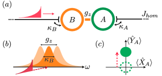
Figure 1: (a) Sketch of a single absorber model for photon detection. A signal photon (red) is absorbed in a mode B and induces a coherent state displacement in a harmonic mode A which is measured using standard homodyne measurement. (b) The coupling between A and B induces fluctuations in the lorentzian absorption spectrum of mode B, preventing the absorbtion of incoming photons. (c) Illustration of phase space for mode A as a photon is absorbed in B.

Basic Principle—First consider the toy model illustrated in Fig. 1(a), where a signal photon (red) traveling along an input waveguide is absorbed into a single “absorber” mode B (orange) at a rate $\kappa_{B}$. This first mode is coupled to a second “measurement” harmonic mode A (green) which decays at a rate $\kappa_{A}$ into an output port continuously measured using a standard homodyne measurement chain (not shown). In this simple toy model, we assume that the two modes are coupled by the longitudinal interaction ($\hbar=1$)

$$\hat{H}_{I}=g_{z}\hat{b}^{\dagger}\hat{b}(\hat{a}+\hat{a}^{\dagger}),$$ (1)

where $\hat{a}$, $\hat{b}$ are the annihilation operators of mode A and B respectively. This interaction implements a textbook photon number measurement: the measured observable $\hat{b}^{\dagger}\hat{b}$ is coupled to the generator of displacement of a pointer state $\hat{X}_{A}=\hat{a}+\hat{a}^{\dagger}$. As schematically illustrated in Fig. 1(c), homodyne measurement of the orthogonal quadrature $\hat{Y}_{A}=-i(\hat{a}-\hat{a}^{\dagger})$ allows to precisely measure the photon number inside the absorber mode B without destroying the photon.

In order to induce a displacement in mode A, a signal photon however needs to first enter the absorber mode B, an unlikely process at large coupling strengths $g_{z}$. Indeed, as schematically illustrated in Fig. 1(b), $\hat{H}_{I}$ induces quantum fluctuations of the absorber’s frequency which can prevent it from absorbing the arriving photon. In order to minimize this unwanted measurement back-action, the width of these fluctuations, compared with the absorber’s linewidth $g_{z}/\kappa_{B}$, should ideally be minimized. On the other hand, the displacement of the measurement mode A, which is given roughly by $g_{z}/\kappa_{B}$ as well, should be maximized to improve the detection efficiency . The optimal quantum efficiency of this toy model is obtained by balancing these two conflicting requirements. Numerically we find an optimal operating point at $g_{z}/\kappa_{B}=1$, the smallest coupling strength for which the induced displacement is distinguishable from the vacuum noise $\langle\hat{Y}_{A}^{2}\rangle_{vacuum}=1$.

Numerical Simulations—To model the signal photon arriving at the detector, a source mode C is introduced, with a frequency matching the absorber mode B, $\omega_{C}=\omega_{B}$. To minimize reflection, we take the signal photon linewidth $\kappa_{C}/\kappa_{B}=0.1$ to be much smaller than the absorber’s linewidth $\kappa_{B}$. Following the experiments of Refs. Houck et al. (2007); Bozyigit et al. (2011), this mode is initialized with one excitation leading to a signal photon emission with an exponentially decaying waveform.

The quantum efficiency of this simple photon detector can be determined by numerically simulating multiple realizations of the above scenario and computing the corresponding homodyne current of the measurement mode A. In practice, this is realized by integrating the stochastic master equation Wiseman and Milburn (2010)

$$\begin{split}d\rho&=\mathcal{L}\rho\,dt+\sqrt{\eta_{h}\kappa_{A}}\mathcal{H}[-i\hat{a}]\rho\,dW,\\ \hat{H}&=\hat{H}_{I}-\frac{i\sqrt{\kappa_{B}\kappa_{C}}}{2}(\hat{c}^{\dagger}\hat{b}-\hat{c}\hat{b}^{\dagger}),\end{split}$$ (2)

where $\hat{c}$ is the annihilation operator of the source mode C and $\mathcal{L}\bullet$ is the Linbladian superoperator $\mathcal{L}\bullet=-i[\hat{H},\bullet]+\sum_{j}\mathcal{D}[\hat{L}_{j}]\bullet$ with $\hat{L}_{1}=\sqrt{\kappa_{A}}\hat{a}$, $\hat{L}_{2}=\sqrt{\kappa_{B}}\hat{b}+\sqrt{\kappa}_{C}\hat{c}$. The combination of the term coupling $\hat{c}$ and $\hat{b}$ in $\hat{H}$ and of the composite decay operator $\hat{L}_{2}$ assures that the output of mode C is cascaded to the input of mode B Gardiner (1993); Carmichael (1993). Moreover, $\eta_{h}$ is the homodyne measurement chain efficiency, $\mathcal{D}[\hat{L}]\bullet=\hat{L}\bullet\hat{L}^{\dagger}-\frac{1}{2}\{\hat{L}^{\dagger}\hat{L},\bullet\}$ is the dissipation superoperator and $\mathcal{H}[\hat{a}]\bullet=\hat{a}\bullet+\bullet\hat{a}^{\dagger}-\langle\hat{a}+\hat{a}^{\dagger}\rangle\bullet$ is the homodyne measurement back-action superoperator. The Wiener process $dW$ is a random variable with the statistical properties $E[dW]=0$ and $E[dW^{2}]=dt$, where $E[\bullet]$ denotes an ensemble average. For each trajectory, the resulting homodyne current is given by $J_{hom}(t)=\sqrt{\eta_{h}\kappa_{A}}\langle\hat{Y}_{A}\rangle+\xi(t)$, where $\xi(t)=dW/dt$ Wiseman and Milburn (2010). Here and below, we use ensembles of $N_{traj}=2000$ trajectories and, to focus solely on the characteristics of the photodetector itself, assume a perfect homodyne detection chain $\eta_{h}=1$.

For each realization of the homodyne current, we consider that a photon is detected if the convolution of the homodyne signal with a filter, $\bar{J}_{hom}(t)=J_{hom}(t)\star f(t)$, exceeds a threshold value $Y_{thr}$, i.e., if $\text{Max}_{t}(\bar{J}_{hom})>Y_{thr}$. To give more weight to times where the signal is, on average, larger, we use $f(t)\propto\langle\hat{Y}_{A}(t)\rangle_{ME}$ computed by averaing Eq. 2 over all trajectories (equivalently, solving the standard unconditional master equation) Fan et al. (2014). Given an ensemble of $N_{traj}$ trajectories, the quantum efficiency is then computed as defined in Ref. Hadfield (2009)

$$\eta=\frac{N_{click}}{N_{traj}},$$ (3)

where $N_{click}$ is the number of trajectories where a photon is detected. Although with this model no prior information about the photon arrival time is needed, if this information is available the measurement can be restricted to a time window of length $\tau_{m}$. In that case, a better metric is the measurement fidelity Sathyamoorthy et al. (2014); Koshino et al. (2013)

$$\mathcal{F}=\frac{1}{2}\left(\eta+1-\Gamma_{dark}\times\tau_{m}\right),$$ (4)

where $\Gamma_{dark}$ is the dark count rate, i.e. the rate at which the detector “clicks” without a signal photon. To maximize the detector repetition rate, $\tau_{m}$ is set to the smallest value that maximizes the fidelity.

For the single absorber model with $g_{z}/\kappa_{B}=1$ and $\kappa_{A}/\kappa_{B}=0.2$, we obtain an efficiency of 79% with $\Gamma_{dark}/\kappa_{B}=1.4\times 10^{-3}$. This translates to a measurement fidelity of $\mathcal{F}=$ 82% for a time window of $\kappa_{B}\tau_{m}=125$. The dead time of the detector after a detection event is given by the reset time of the measurement mode A back to vacuum. This corresponds to several decay times $1/\kappa_{A}$ or, alternatively, can be significantly speed-up by using active cavity reset approaches McClure et al. (2016); Bultink et al. (2016); Boutin et al. (2016).

This scheme is similar to previously studied models Helmer et al. (2009); Fan et al. (2014); Milburn and Basiri-Esfahani (2015) and, although it leads to relatively large detection fidelities, the resulting displacement of mode A is small, $\langle\hat{Y}_{A}\rangle\sim g_{z}/\kappa_{B}=1$. In this situation, adding an imperfect homodyne measurement chain, $\eta_{h}<1$, will lead to a significant reduction of the quantum efficiency.

Atom Ensemble—As already pointed out, the key issue with using a single absorber is that both the total displacement of the measurement mode A and the measurement back-action on B scale with $g_{z}/\kappa_{B}$. This is a direct consequence of the fact that the time spent in a simple resonant system is given by the inverse of its bandwidth. In order to increase the quantum efficiency, we thus present a scheme where the interaction time with the photon is increased while keeping the ratio $g_{z}/\kappa_{B}$ constant.

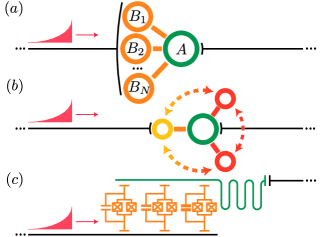
Figure 2: (a) The single absorber B is replaced by an ensemble of inhomogeneous modes coupled at the same point of the input waveguide. (b) Redrawing of (a) in the bright and dark states basis for $N=3$. The incoming photon is absorbed into a bright state (yellow) and then passively transferred to dark states (dark orange). (c) Possible circuit QED implementation for $N=3$. Tunable transmon qubits acting as absorbers are coupled capacitively on one side to an input transmission line and on the other side to a measurement resonator.

As schematically illustrated in Fig. 2(a), we first replace the single absorber by a small ensemble of $N\lesssim 5$ artificial atoms and, second, we inhomogeneously detune each atom with respect to the average ensemble frequency. By connecting these absorbers approximately to the same point of the input waveguide , we induce the creation of a superradiant bright state $\hat{b}_{+}=1/\sqrt{N}\sum_{i}\hat{b}_{i}$ and dissipationless dark states Lalumière et al. (2013); van Loo et al. (2013). Moreover, we assume that the absorbers are coupled to the measurement mode A such that the measured observable is $\hat{N}_{B}=\sum_{i}\hat{b}^{\dagger}_{i}\hat{b}_{i}$, the total photon number in the ensemble. In this case, the ideal interaction picture Hamiltonian becomes

$$\hat{H}_{I}^{E}=g_{z}\hat{N}_{B}\hat{X}_{A}+\sum_{i=1}^{N}\Delta_{i}\hat{b}^{\dagger}_{i}\hat{b}_{i},$$ (5)

where $\Delta_{i}=\omega_{Bi}-\omega_{B}\lesssim\kappa_{B}$ is the detuning of the $i^{th}$ atom with respect to the average frequency of the ensemble $\omega_{B}=\sum_{i}\omega_{Bi}/N$ and the first term represents the direct generalization of Eq. 1 for an ensemble of atoms.

In this model, an incoming signal photon is absorbed in the collective bright state $\hat{b}_{+}$ at a rate scaling linearly with $N$. Without loss of generality and to fix the effective collective absorption rate of the detector at $\kappa_{B}$, we choose the bare linewidth of the atoms to be $\kappa_{Bi}=\kappa_{B}/N$. In the case where the atoms are on resonance $\Delta_{i}=0\,\forall\,i$, the bright and dark subspaces are uncoupled and the model becomes equivalent to the single absorber model illustrated in Fig. 1(a) Fan et al. (2013).

On the other hand, non-homogeneous detunings $\Delta_{i}\neq\Delta_{j}$ lead to coupling of the bright and dark subspaces. If this coupling is carefully adjusted, a signal photon can then be absorbed into the bright state, transferred to a long-lived dark state and, after some time $\tau_{trap}$, return to the bright state where it is re-emitted. Figure 2(b) illustrates this process schematically with the $\hat{b}_{+}$ bright state (yellow) being coupled to $N-1$ dark states (dark orange). Crucially, changing the detunings affects neither the coupling strength $g_{z}$ nor the effective linewidth $\kappa_{B}$, which means that the measurement back-action should not be affected either. On the other hand, the total displacement induced in the measurement mode A is changed from $g_{z}/\kappa_{B}$ to roughly $g_{z}\times(1/\kappa_{B}+\tau_{trap})$. As a result, by increasing $\tau_{trap}$ and reducing $g_{z}$, we can thus, as desired, significantly increase the quantum efficiency by simultaneously increasing the induced displacement and reducing the measurement back-action. In practice, $\tau_{trap}$ can be made longer by increasing the number of absorbers and optimizing the detunings, $\vec{\Delta}$, accordingly SM .

We perform full stochastic master equation simulations using Eq. 2 with the replacements $\hat{b}\rightarrow\hat{b}_{+}$, $\hat{H}_{I}\rightarrow\hat{H}_{I}^{E}$ and show the increase in measurement fidelity, $\mathcal{F}$, as a function of ensemble size in Fig. 3(a). As shown in panel (b), for $N=4$, a quantum efficiency of $\eta=92\%$ is obtained at a very low estimated dark count rate of $\Gamma_{dark}/\kappa_{B}=7\times 10^{-6}$. For a time window of $\kappa_{B}\tau_{m}=126$ this translates to the measurement fidelity of $\mathcal{F}=96\%$ observed in panel (a). As also illustrated in panel (b), it is possible to vary the threshold $Y_{thr}$ to trade a higher dark count rate for a higher efficiency, or the converse. Here, the dark count rate $\Gamma_{dark}$ is computed from trajectories with no signal photon (full lines) and, where it is too small to be precisely calculated from trajectories, estimated from time correlations in the filtered signal from vacuum (colored dashed lines) SM .

Importantly, due to the increased interaction time, the measured homodyne signal increases with $N$ and, for $N=4$, is already much larger than vacuum noise. As a result, the detector becomes increasingly robust to potential imperfections in the homodyne detection chain $\eta_{h}<1$. We, moreover, expect the quantum efficiency to continue increasing as the number of absorbers is raised above 4. Unfortunately, for $N\geq 5$, the required Hilbert space size for numerical simulations is impractically large. We note, however, that at $N=4$ the performance are already close to an expected maximum of $\eta_{\text{max}}\sim 96\%$ indicated by the black dashed line in panels (a) and (b). This upper bound is due to high frequency components of the signal photon that are directly reflected from the absorber and thus do not lead to a detectable signal in mode A SM . The value of this upper bound is linked to the choice of both detector and signal photon parameters and could be improved upon further optimization.

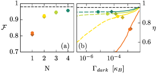
Figure 3: (a) Fidelity as a function of the number of absorbers. The full circles are calculated using the ideal model with $\kappa_{A}/\kappa_{B}=0.2$, $g_{z}^{(1)}/\kappa_{B}=1$, $g_{z}^{(2)}/\kappa_{B}=0.6$, $g_{z}^{(3)}/\kappa_{B}=0.5$, $g_{z}^{(4)}/\kappa_{B}=0.4$ with the detunings $\vec{\Delta}^{(2)}/\kappa_{B}=(0.55,\,-0.55)$, $\vec{\Delta}^{(3)}/\kappa_{B}=(0.7,\,-0.7,\,0)$ and $\vec{\Delta}^{(4)}/\kappa_{B}=(0.7,\,-0.7,\,0.23,\,-0.23)$. The diamonds were calculated using realistic parameters for an ensemble of transmons dispersively coupled to a resonator with $\kappa_{B}/2\pi=10$ MHz, $g_{z}/\chi=10$ and $T_{1},T_{2}=30\,\mu s$. (b) Efficiency of the detector as a function the dark count rate. The solid lines correspond to statistics extracted from trajectories while for the dashed lines $\Gamma_{dark}$ was estimated using an analytical formula. The lines were calculated for the ideal model and the points indicate where the fidelity is maximized. The black dashed line in both panels correspond the upper bound $\eta_{max}$ imposed by the photon shape used here.

Since our proposal is continuous, the time $\tau_{c}$ at which the homodyne signal crosses the threshold reveals information about the photon arrival time. Fig. 4 shows histograms of the normalized number of counts for $\tau_{c}$, as recorded from trajectories where a photon is detected. In Fig. 4(a), the number of absorbers is varied and the signal threshold, $Y_{thr}$, is set to optimize the fidelity (see Fig. 3). On the other hand, in Fig. 4(b), we set $N=4$ and vary the threshold. In both panels, the input photon shape (red) is shown for comparison. As the threshold increases, the distribution of crossing times narrows and the precision on the arrival time of the photon therefore increases. As mentioned above, increasing $N$ leads to larger homodyne signals. Hence, adding more absorbers allows to increase the threshold which, in turn, improves the arrival time precision. Moreover, since $1/\kappa_{C}$ is the longest timescale in these simulations, at $N=4$ the photon shape can be resolved from the histogram. The mismatch between the distribution and the red line near $\kappa_{B}t=0$ is due to the sharp, high frequency feature of the input photon that is reflected from the absorbers without detection.

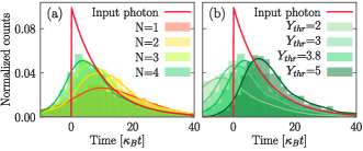
Figure 4: (a) Normalized number of detection events as a function of time for different number of absorbers in the ideal model Eq. 5. (b) Normalized number of counts for different thresholds for $N=4$. $Y_{thr}=3.8$ is the threshold that maximizes the fidelity in Fig. 3. In both panels, the input photon shape (red) is shown for comparison and an arbitrary time offset has been substracted from the homodyne signal.

Physical implementation—A possible implementation of this model, based on dispersive coupling of transmon qubits, is illustrated in Fig. 2(c). Here, an ensemble of superconducting transmon qubits is capacitively coupled on one side to a transmission line and on the other side to a measurement resonator (mode A). The coupling strength to the resonator is denoted $g$. We take a large detuning between the qubits center frequency $\omega_{B}$ and the resonator frequency $\Delta_{r}=\omega_{r}-\omega_{B}\gg\kappa_{A},\kappa_{B},g$ and use the standard dispersive approximation SM . The absorption of a signal photon by the qubits induces a shift in the resonator frequency which is detected by continuously probing the resonator with a coherent drive corresponding to a field amplitude $\alpha$ Blais et al. (2004). In this situation, we find that the system of Fig. 2(c) is well described by the displaced dispersive Hamiltonian SM

$$\hat{H}_{\chi}^{D}=g_{z}\hat{N}_{B}\hat{X}_{A}+\sum_{i=1}^{N}\Delta_{i}\hat{b}^{\dagger}_{i}\hat{b}_{i}+2\chi\hat{N}_{B}\hat{a}^{\dagger}\hat{a}+\Delta_{+}\hat{b}^{\dagger}_{+}\hat{b}_{+},$$ (6)

where $\chi$ is the usual transmon dispersive shifts Koch et al. (2007); SM , $g_{z}=2\chi\alpha$, and $\Delta_{+}$ results from a combination of the resonator-induced Lamb shift and spurious qubit-qubit coupling SM . The first two terms correspond exactly to the ideal model Hamiltonian Eq. 5, while the two additional last terms are small and imposed by this specific implementation.

For a fixed coupling strength $g_{z}$, the quantum efficiency is maximized for a small dispersive shift $\chi$ and a large $\alpha$. However, the dispersive approximation used here is only valid at low photon numbers, imposing an upper bound for the resonator steady state displacement $|\alpha|$. As shown by the diamonds in Fig. 3, working with $\alpha=5$, we numerically find that the two additional terms in Eq. 6 have a minimal impact on the quantum efficiency. Moreover, it is possible to mitigate the detrimental effect of a small $\Delta_{+}$ by adjusting the detunings $\vec{\Delta}$.

As an example, choosing realistic parameters $N=4$, $\kappa_{B}/2\pi=10\text{ MHz}$, $\kappa_{A}/2\pi=2\text{ MHz}$, $\chi/2\pi=0.4\text{ MHz}$, $\alpha=5$, $\vec{\Delta}/2\pi=(6.6,\,-7.4,\,2.3,\,-2.3)\text{ MHz}$ and using state-of-the-art transmon decoherence times $T_{1},T_{2}=30\,\mu s$ McKay et al. (2016), we obtain $\eta=92\%$ with $\Gamma_{dark}=4.2\times 10^{-3}\mu s^{-1}$. Given a time window of $\tau_{m}=2\,\mu s$, this corresponds to a large measurement fidelity of $\mathcal{F}=96\%$.

Conclusion—We have presented a high-efficiency, non-destructive scheme for itinerant microwave photon detection where no prior information about the arrival time of the photon is needed. This scheme is based on the continuous measurement of the photon number in an ensemble of inhomogeneous artificial atoms where the photon can be stored for long times due to the existence of long-lived dark states. We also presented a realistic physical implementation of this idea using an ensemble of transmon qubits dispersively coupled to a single resonator. Using only four transmons, we estimate that fidelities as high as 96% are attainable for the photon shape considered here.

Given that the output signal is proportional to the total number of photons inside the absorbers, the same model could potentially to be used as a photon-number resolving detector. Future work will investigate this possibility. Finally, we note that the same scheme could be applicable to non-destructive detection of single itinerant phonons by coupling the transmons to surface acoustic waves Gustafsson et al. (2014); Manenti et al. (2017).

See pages 1 of SM_PD.pdf See pages 2 of SM_PD.pdf See pages 3 of SM_PD.pdf See pages 4 of SM_PD.pdf See pages 5 of SM_PD.pdf See pages 6 of SM_PD.pdf See pages 7 of SM_PD.pdf See pages 8 of SM_PD.pdf See pages 9 of SM_PD.pdf See pages 10 of SM_PD.pdf