Bilinear quantum systems on compact graphs: well-posedness and global exact controllability

Abstract

A major application of the mathematical concept of graph in quantum mechanics is to model networks of electrical wires or electromagnetic wave-guides. In this paper, we address the dynamics of a particle trapped on such a network in presence of an external electromagnetic field. We study the controllability of the motion when the intensity of the field changes over time and plays the role of control. From a mathematical point of view, the dynamics of the particle is modeled by the so-called bilinear Schrödinger equation defined on a graph representing the network. The main purpose of this work is to extend the existing theory for bilinear quantum systems on bounded intervals to the framework of graphs. To this end, we introduce a suitable mathematical setting where to address the controllability of the equation from a theoretical point of view. More precisely, we determine assumptions on the network and on the potential field ensuring its global exact controllability in suitable spaces. Finally, we discuss two applications of our results and their practical implications to two specific problems involving a star-shaped network and a tadpole graph.

1 Introduction

During the last decades, graph type models (Figure 1) have been extensively studied in the literature for the modeling of phenomena arising in science, social sciences and engineering. Applications to the quantum mechanics include the study of the dynamics of free electrons in organic molecules starting from the seminal work [Pau36] (see also [Kuh48, Pla49, RS53, Sla17, Wil67]), the superconductivity in granular and artificial materials [Ale83], acoustic and electromagnetic wave-guides networks in [FJK87, ML71], etc.

Figure 1: A compact graph is a one-dimensional domain composed by finite vertices (points) connected by edges (segments) of finite lengths.

The aim of this paper is to study the dynamics of a particle trapped on a network of wires, or wave-guides, in presence of an electromagnetic external field. We assume that the particle is subjected to zero resistance when it crosses the nodes of the network. The intensity of the external field is a function of the time and it plays the role of control. The dynamics of the particle is driven by the bilinear Schrödinger equation in $L^{2}(\mathscr{G},\mathbb{C})$ where $\mathscr{G}$ is the graph modeling the network:

(BSE) $$\begin{split}\begin{cases}i\partial_{t}\psi(t)=A\psi(t)+u(t)B\psi(t),\ \ \ \ \ \ \ \ &t\in(0,T),\\ \psi(0)=\psi_{0},\ &\ \ \ \ T>0.\\ \end{cases}\end{split}$$

The term $u(t)B$ in the (BSE) represents the external field acting on the system. The bounded symmetric operator $B$ describes the action of the field and $u\in L^{2}((0,T),\mathbb{R})$ its intensity. The operator $A=-\Delta$ is a self-adjoint Laplacian equipped with suitable boundary conditions (see the next paragraphs for further details).

The mathematical analysis of self-adjoint operators on networks was addressed in [RS53] by Ruedenber and Scherr (see also [RB72]). There, they studied the dynamics of specific electrons in the conjugated double-bounds organic molecules. In such a context, some electrons behave as if they were trapped on a network of wave-guides. The graphs are obtained as the idealization of these structures in the limit where the diameter of their section is much smaller than the length. A similar approach was developed by Saito in [Sai00, Sai01] where the graphs are obtained as “shrinking” domains. For analogous ideas, we refer to the papers [RS01, Ola05].

A natural question on the (BSE) of high relevance for the mentioned applications is whether it is possible to control the motion of the particle through the network by varying the intensity of the external field. From a mathematical point of view, we wonder if for any couple of quantum states $\psi_{0}$ and $\psi_{1}$, there exists a control $u$ so that the solution of the (BSE) with initial state $\psi_{0}$ reaches, or at least approaches, $\psi_{1}$.

A peculiarity of the bilinear quantum systems as (BSE) is that their exact controllability can not be ensured in the Hilbert space where the dynamics is defined when $B$ is a bounded operator. This is a consequence of the results developed by Ball, Mardsen and Slemrod in the work on bilinear systems [BMS82].

For the bilinear Schrödinger equation (BSE) on the interval $\mathscr{G}=(0,1)$, a successful strategy was developed by Beauchard in [Bea05] which addresses the exact controllability in suitable subspaces of $L^{2}((0,1),\mathbb{C})$. Beauchard studied the equation with $A$ the Dirichlet Laplacian $-\Delta_{D}$ on $(0,1)$ and proved the local exact controllability in $D(|\Delta_{D}|^{\frac{3}{2}})$. This method was later exploited in [BL10, Mor14, MN15, Duc19, Duc20].

Even though the global exact controllability of the bilinear Schrödinger equation (BSE) on $\mathscr{G}=(0,1)$ is well-established, the result on networks is still an open problem to the best of our knowledge.

• Firstly, it is not clear which is the “good” space where to consider the dynamics. When $A$ is a self-adjoint Laplacian on a compact graph, it is not easy to characterize how the boundary conditions defining the domains $D(|A|^{\frac{s}{2}})$ are affected by the variation of the parameter $s>0$.

• From a spectral point of view, even though $A$ admits compact resolvent (see Remark 2.1), its ordered eigenvalues $(\lambda_{k})_{k\in\mathbb{N}^{*}}$ are not explicit up to very specific situations, unlike the Dirichlet Laplacian $-\Delta_{D}$ on $(0,1)$ (we refer to Remark 3.8 for further details on the subject). In general, a more complicated structure of the networks entails increased difficulties in determining the spectral behavior.

• Finally, the techniques developed in the works [Bea05, BL10, Duc20, Duc19, Mor14] can not be directly applied for the (BSE) on compact graphs $\mathscr{G}$. Indeed, the only sure fact on $(\lambda_{k})_{k\in\mathbb{N}^{*}}$ is that the uniform spectral gap $\inf_{{k\in\mathbb{N}^{*}}}|\lambda_{k+1}-\lambda_{k}|>0$ can be only guaranteed when $\mathscr{G}=(0,1)$. This hypothesis is crucial for the techniques developed in the mentioned works.

The purpose of this work is threefold. First, we introduce a suitable mathematical framework where to consider the dynamics of the (BSE) and we characterize the Sobolev’s spaces $D(|A|^{\frac{s}{2}})$ with $s\geq 0$. Second, we study the well-posedness of the (BSE) in such domains for very specific values of the parameter $s$. Third, we develop a new technique leading to the global exact controllability of the (BSE) in these spaces.

Our main result yields the global exact contrability for bilinear quantum systems on network under fairly general hypotheses on the spectrum $A$ and on the potential $B$. We infer the validity of the mentioned spectral assumptions for suitable networks shaped as: star graphs, double-ring graphs, tadpole graphs or two-tails tadpole graphs (Figure 2). In the following paragraph, we provide an explicit potential field $B$ acting on a star-shaped network so that the controllability is guaranteed. In Section 3.3, we treat another specific problem on a network modeled by a tadpole graph.

Figure 2: The figure respectively represents a star graph, a double-ring graph, a tadpole graph and a two-tails tadpole graph.

Star-shaped network

Let us consider a network of $3$ branches connected in one node. We can assume it is a structure of electrical wires or a system of wave-guides representing the so-called “branching points” in the conjugated double-bounds organic molecules (see [RS53] by Ruedenber and Scherr). We represent the network with a star-graph $\mathscr{G}$ composed by $3$ edges $\{e_{1},e_{2},e_{3}\}$. We denote by $v$ the internal vertex connecting all the edges of $\mathscr{G}$. We parametrize each $e_{j}$ with a coordinate going from $0$ to its length $L_{j}$ in $v$ (see Figure 3).

Figure 3: The figure shows the parametrization of a star graph with $3$ edges.

We consider a particle trapped on such a network and we represent it by a quantum state $\psi=(\psi^{1},\psi^{2},\psi^{3})\in L^{2}(\mathscr{G},\mathbb{C}):=\prod_{j=1}^{3}L^{2}(e_{j},\mathbb{C}),$ where each $\psi^{j}:e_{j}\rightarrow\mathbb{C}$ describes the probability of particle to be located in the edge $e_{j}$. We assume that an external field acts on the network as a sufficiently regular potential field $\mu$ localized on the branch represented by $e_{1}$ and with time-dependent intensity. We model the field as $u(t)B$ where

(1) $$u\in L^{2}((0,T),\mathbb{R}),\ \ \ \ \ \ \ \ \ B:\psi=(\psi^{1},\psi^{2},\psi^{3})\in L^{2}(\mathscr{G},\mathbb{C})\longmapsto\big{(}\mu(x)\psi^{1},0,0\big{)}.$$

The dynamics of the particle in the time $(0,T)$ is modeled by the bilinear Schrödinger equation in $L^{2}(\mathscr{G},\mathbb{C})$

(2) $$\begin{split}\begin{cases}i\partial_{t}\psi^{1}(t,x)=-\partial_{x}^{2}\psi^{1}(t,x)+u(t)\mu(x)\psi^{1}(t,x),\ \ \ \ \ \ \ \ &t\in(0,T),\ x\in(0,L_{1}),\\ i\partial_{t}\psi^{2}(t,x)=-\partial_{x}^{2}\psi^{2}(t,x),\ \ \ \ \ \ \ \ &t\in(0,T),\ x\in(0,L_{2}),\\ i\partial_{t}\psi^{3}(t,x)=-\partial_{x}^{2}\psi^{3}(t,x),\ \ \ \ \ \ \ \ &t\in(0,T),\ x\in(0,L_{3}),\\ \end{cases}\end{split}$$

endowed with the following boundary conditions

(3) $$\begin{split}\psi^{1}(L_{1})=\psi^{2}(L_{2})=&\ \psi^{3}(L_{3}),\ \ \ \ \ \ \ \ \ \ \ \ \partial_{x}\psi^{1}(L_{1})+\partial_{x}\psi^{2}(L_{2})+\partial_{x}\psi^{3}(L_{3})=0,\\ &\psi^{1}(0)=\psi^{2}(0)=\psi^{3}(0)=0.\\ \end{split}$$

The identities appearing in the first line of (3) model the peculiarity of the central node of the network to act zero resistence on the crossing particle (see [RS53, RB72]) and they are encoded by Neumann-Kirchhoff boundary conditions. The last identities are the classical Dirichlet boundary conditions. Let

$$H^{s}:=\prod_{k=1}^{3}H^{s}(e_{k},\mathbb{C})$$

for $s>0$. We denote by $-\Delta$ the Laplacian operator appearing in (2)-(3), i.e.

$$D(-\Delta)=\Big{\{}\psi=(\psi^{1},\psi^{2},\psi^{3})\in H^{2}\ :\ \psi\ \text{verifies the boundary conditions }\eqref{mainxS_boundaries}\Big{\}}.$$

Definition 1.1.

Let $N\in\mathbb{N}^{*}$. We denote by $\mathcal{A}\mathcal{L}(N)$ the set of elements $\{L_{j}\}_{j\leq N}\in(\mathbb{R}^{+})^{N}$ so that $\big{\{}1,L_{1},...,L_{N}\big{\}}$ are linearly independent over $\mathbb{Q}$ and all the ratios $L_{k}/L_{j}$ are algebraic irrational numbers.

The set $\mathcal{A}\mathcal{L}(N)$ with $N\in\mathbb{N}^{*}$ contains the uncountable set of $\{L_{j}\}_{j\leq N}\in(\mathbb{R}^{+})^{N}$ such that each $L_{j}$ can be written in the form $t\widetilde{L}_{j}$ where all the ratios $\widetilde{L}_{j}/\widetilde{L}_{k}$ are algebraic irrational numbers and $t$ is a transcendental number. For instance, $\{\pi\sqrt{2},\pi\sqrt{3}\}$ belongs to $\mathcal{A}\mathcal{L}(2)$, while $\{\pi,\pi\sqrt{2},\pi\sqrt{3}\}$ to $\mathcal{A}\mathcal{L}(3)$.

Theorem 1.2.

Let $\mu:x\in(0,L_{1})\longmapsto(x-L_{1})^{4}$. There exists $\mathcal{C}\subset(\mathbb{R}^{+})^{3}$ countable such that, for every $\{L_{1},L_{2},L_{3}\}\in\mathcal{A}\mathcal{L}(3)\setminus\mathcal{C}$, the dynamics of the system (2)-(3) is globally exactly controllable in

$$H^{4+\epsilon}\cap D(|\Delta|^{2}),\ \ \ \ \ \ \ \ \epsilon>0.$$

In other words, let $\Gamma_{T}^{u}$ be the unitary propagator associated to the dynamics of (2)-(3) in the time interval $(0,T)$ with control $u\in L^{2}((0,T),\mathbb{R})$. For every $\psi^{1},\psi^{2}\in H^{4+\epsilon}\cap D(|\Delta|^{2})$ such that $\|\psi^{1}\|_{L^{2}(\mathscr{G},\mathbb{C})}=\|\psi^{2}\|_{L^{2}(\mathscr{G},\mathbb{C})}$,

$$\exists T>0,\ \ \ u\in L^{2}\big{(}(0,T),\mathbb{R}\big{)}\ \ \ :\ \ \ \Gamma_{T}^{u}\psi^{1}=\psi^{2}.$$

Theorem 1.2 is proved in Section 3.2 and it is a consequence of the abstract result of Theorem 3.2. There, the statement is guaranteed when specific hypotheses on the spectral behaviour of $A$ and on the field $B$ are satisfied.

Theorem 1.2 yields that the controllability of (2)-(3) holds even though the external field only acts on the edge $e_{1}$. When the particle, represented by a state $\psi_{0}$, is (mostly) localized in $e_{3}$, it is still possible to move it to any other edge of the network by controlling the intensity of the field (Figure 4).

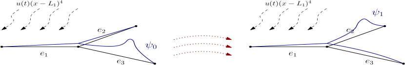
Figure 4: The figure represents an interesting application of Theorem 1.2: it is possible to steer any state $\psi_{0}$, localized in $e_{3}$, to any other state $\psi_{1}$, localized in $e_{2}$, by means of the dynamics of the bilinear Schrödinger equation (2)-(3), even though the potential field $u(t)\mu(x)=u(t)(x-L_{1})^{4}$ only acts on the edge $e_{1}$.

This peculiarity follows from the choice of $\{L_{1},L_{2},L_{3}\}\in\mathcal{A}\mathcal{L}(3)$. In this case, each bounded state of $i\partial_{t}\psi=-\Delta\psi$ is supported by the whole network (see Remark 3.6) and then, it is affected by the field acting on $e_{1}$. As a consequence, when we see $\psi_{0}$ as a superposition of bounded states, we realize that the control field “see” the particle even though it is localized on a different edge from $e_{1}$.

Remark 1.3.

If $L_{2}/L_{3}$ is rational, then there exist eigenfunctions of $-\Delta$ vanishing in $e_{1}$. When $L_{1}/L_{3}$ is also rational, the spectrum of $-\Delta$ presents multiple eigenvalues (see Remark 3.6). These are obvious obstructions to the controllability of (2)-(3) since the potential only acts on $e_{1}$. As a consequence, when we change the lengths of the branches of the network, it may happen that the controllability of (2)-(3) is lost, even though the set of the ”uncontrollable” lengths is countable.

Scheme of the work

In Section 2, we present the mathematical framework and the notations adopted in the work. In Section 3, we state with Theorem 3.2 our abstract global exact controllability result which we use to prove Theorem 1.2. In the final part of this section, we also deal with a specific problem involving a tadpole graph. In Section 4, we present some interpolation properties for the domains $D(|A|^{\frac{s}{2}})$ with $s>0$ and we ensure the well-posedness of the (BSE). In Section 5, we prove the abstract result of Theorem 3.2 by extending a local exact controllability. In Appendix A, we ensure some spectral proprieties adopted in the manuscript. In Appendix B, we provide a new technique leading to the solvability of the so-called moment problem appearing in the proof of the local exact controllability. In Appendix C, we develop some perturbation theory techniques.

2 Preliminaries

2.1 Mathematical framework and notations

Let $\mathscr{G}$ be a compact graph composed by $N\in\mathbb{N}^{*}$ edges $\{e_{j}\}_{j\leq N}$ of lengths $\{L_{j}\}_{j\leq N}$ and $M\in\mathbb{N}^{*}$ vertices $\{v_{j}\}_{j\leq M}$. For every vertex $v$, we denote

(4) $$N(v):=\big{\{}l\in\{1,...,N\}\ |\ v\in e_{l}\big{\}},\ \ \ \ \ \ n(v):=|N(v)|.$$

We call $V_{e}$ and $V_{i}$ the external and the internal vertices of the graph $\mathscr{G}$ (see Figure 5).

Figure 5: Internal and external vertices in a compact graph.

We study graphs equipped with a metric, which parametrizes each edge $e_{j}$ with a coordinate going from $0$ to its length $L_{j}$. A graph is compact when it is composed by a finite number of vertices and edges of finite lengths. We consider functions $f:=(f^{1},...,f^{N}):\mathscr{G}\rightarrow\mathbb{C}$ with domain a compact metric graph $\mathscr{G}$ so that $f^{j}:e_{j}\rightarrow\mathbb{C}$ for every $j\leq N$. We denote

$$L^{2}(\mathscr{G},\mathbb{C})=\prod_{j\leq N}L^{2}(e_{j},\mathbb{C}).$$

The Hilbert space $L^{2}(\mathscr{G},\mathbb{C})$ is equipped with the norm $\|\cdot\|_{L^{2}}$ induced by the scalar product

$$\langle\psi,\varphi\rangle_{L^{2}}:=\sum_{j\leq N}\langle\psi^{j},\varphi^{j}\rangle_{L^{2}(e_{j},\mathbb{C})}=\sum_{j\leq N}\int_{e_{j}}\overline{\psi^{j}}(x)\varphi^{j}(x)dx,\ \ \ \ \ \ \forall\psi,\varphi\in L^{2}(\mathscr{G},\mathbb{C}).$$

For $s>0$, we define the spaces

$$H^{s}=H^{s}(\mathscr{G},\mathbb{C}):=\prod_{j=1}^{N}H^{s}(e_{j},\mathbb{C}),\ \ \ \ \ \ \ h^{s}=\Big{\{}(x_{j})_{j\in\mathbb{N}^{*}}\subset{\mathbb{C}}\ \big{|}\ \sum_{j=1}^{\infty}|j^{s}x_{j}|^{2}<\infty\Big{\}}.$$

We equip $h^{s}$ with the norm $\big{\|}(x_{j})_{j\in\mathbb{N}^{*}}\big{\|}_{(s)}=\big{(}\sum_{j=1}^{\infty}|j^{s}x_{j}|^{2}\big{)}^{\frac{1}{2}}$ for every $(x_{j})_{j\in\mathbb{N}^{*}}\in h^{s}$. Let $f\in H^{1}$ and $v$ be a vertex of $\mathscr{G}$ connected once to an edge $e_{j}$ with $j\leq N$. When the coordinate parametrizing $e_{j}$ in the vertex $v$ is equal to $0$ (resp. $L_{j}$), we denote

(5) $$\partial_{x}f^{j}(v)=\partial_{x}f^{j}(0),\ \ \ \ \ \ \ \ \big{(}\text{resp.}\ \partial_{x}f^{j}(v)=-\partial_{x}f^{j}(L_{j})\big{)}.$$

When $e_{j}$ is a loop and it is connected to $v$ in both of its extremes, we use the notation

(6) $$\partial_{x}f^{j}(v)=\partial_{x}f^{j}(0)-\partial_{x}f^{j}(L_{j}).$$

When $v$ is an external vertex and then $e_{j}$ is the only edge connected to $v$, we call $\partial_{x}f(v)=\partial_{x}f^{j}(v).$

In the bilinear Schrödinger equation $(\ref{mainx1})$, we consider the Laplacian $A$ being self-adjoint and we denote $\mathscr{G}$ as quantum graph. From now on, when we introduce a quantum graph $\mathscr{G}$, we implicitly define on $\mathscr{G}$ a self-adjoint Laplacian $A$. Formally, $D(A)$ is characterized by the following boundary conditions.

Vertex boundary conditions.

Let $\mathscr{G}$ be a compact quantum graph.

• A vertex $v\in V_{e}$ is equipped with Dirichlet boundary conditions when $f(v)=0$ for every $f\in D(A)$.

• A vertex $v\in V_{e}$ is equipped with Neumann boundary conditions when $\partial_{x}f(v)=0$ for every $f\in D(A)$.

• A vertex $v\in V_{i}$ is equipped with Neumann-Kirchhoff boundary conditions when every $f\in D(A)$ is continuous in $v$ and $\sum_{j\in N(v)}\partial_{x}f^{j}(v)=0$ (according to the notations (5) and (6)).

Graph boundary conditions.

Let $\mathscr{G}$ be a compact quantum graph.

• The graph $\mathscr{G}$ is said to be equipped with ($\mathcal{D}$) when the Laplacian $A=-\Delta$ in $L^{2}(\mathscr{G},\mathbb{C})$ is such that

  $$D(A)=\{\psi\in H^{2}\ :\ \psi\text{ satisfies $(\mathcal{N}\mathcal{K})$ in every $v\in V_{i}$ and ($\mathcal{D}$) in each $v\in V_{e}$}\}.$$

• The graph $\mathscr{G}$ is said to be equipped with ($\mathcal{N}$) when the Laplacian $A=-\Delta$ in $L^{2}(\mathscr{G},\mathbb{C})$ is such that

  $$D(A)=\{\psi\in H^{2}\ :\ \psi\text{ satisfies $(\mathcal{N}\mathcal{K})$ in every $v\in V_{i}$ and ($\mathcal{N}$) in each $v\in V_{e}$}\}.$$

• The graph $\mathscr{G}$ is said to be equipped with ($\mathcal{D}$/$\mathcal{N}$) when the Laplacian $A=-\Delta$ in $L^{2}(\mathscr{G},\mathbb{C})$ is such that

  $$D(A)=\{\psi\in H^{2}\ :\ \psi\text{ satisfies $(\mathcal{N}\mathcal{K})$ in every $v\in V_{i}$ and each $v\in V_{e}$ verifies ($\mathcal{D}$) or ($\mathcal{N}$)}\}.$$

Remark 2.1.

When the boundary conditions described above are satisfied, the Laplacian $A$ is self-adjoint (see [Kuc04, Theorem 3]), it admits compact resolvent and then purely discrete spectrum (see [Kuc04, Theorem 18]).

We denote by $(\lambda_{k})_{k\in\mathbb{N}^{*}}$ the ordered sequence of eigenvalues of $A$ and $(\phi_{k})_{k\in\mathbb{N}^{*}}$ is a Hilbert basis of $L^{2}(\mathscr{G},\mathbb{C})$ composed by corresponding eigenfunctions. Let $[r]$ be the entire part of a number $r\in\mathbb{R}$. For $s>0$, we denote

$$\begin{split}H^{s}_{\mathcal{N}\mathcal{K}}:=\Big{\{}&\psi\in H^{s}(\mathscr{G},\mathbb{C})\ \Big{|}\ \partial_{x}^{2n}\psi\text{ is continuous in }v,\ \forall n\in\mathbb{N},\ n<\big{[}({s+1})/{2}\big{]},\ \forall v\in V_{i};\\ &\sum_{j\in N(v)}\partial_{x}^{2n+1}\psi^{j}(v)=0,\ \forall n\in\mathbb{N},\ n<\big{[}{s}/{2}\big{]},\ \forall v\in V_{i}\Big{\}},\\ H^{s}_{\mathscr{G}}&:=D(A^{{s}/{2}}),\ \ \ \ \ \ \ \ \ \ \ \ \ \ \|\cdot\|_{(s)}:=\|\cdot\|_{H^{s}_{\mathscr{G}}}=\Big{(}\sum_{k\in\mathbb{N}^{*}}\big{|}k^{s}\langle\cdot,\phi_{k}\rangle_{L^{2}}\big{|}^{2}\Big{)}^{\frac{1}{2}}.\\ \end{split}$$

2.2 Spectral properties

The following proposition rephrases the results of [BK13, Theorem  3.1.8] and [BK13, Theorem  3.1.10]. There, we denote by $\big{(}\lambda_{k}^{\widehat{\mathscr{G}}}\big{)}_{k\in\mathbb{N}^{*}}$ the ordered sequence of eigenvalues of $A$ on a compact quantum graph $\widehat{\mathscr{G}}$.

Proposition 2.2.

[BK13, Theorem  3.1.8] & [BK13, Theorem  3.1.10] Let $\mathscr{G}$ be a compact quantum graph.

1) Let $w$ be a vertex of $\mathscr{G}$. If $\mathscr{G}^{\mathcal{D}}$is the graph obtained by changing the boundary conditions in $w$ with ($\mathcal{D}$), then

$$\lambda_{k}^{\mathscr{G}}\leq\lambda_{k}^{\mathscr{G}^{\mathcal{D}}}\leq\lambda_{k+1}^{\mathscr{G}},\ \ \ \ \ \ \ \ k\in\mathbb{N}^{*}.$$

2) Let $w$ and $v$ be two vertices of $\mathscr{G}$ equipped with ($\mathcal{N}\mathcal{K}$) or ($\mathcal{N}$). If $\mathscr{G}^{\prime}$ is the graph obtained by merging the vertices $w$ and $v$ of $\mathscr{G}$ in one unique vertex equipped with ($\mathcal{N}\mathcal{K}$), then

$$\lambda_{k}^{\mathscr{G}}\leq\lambda_{k}^{\mathscr{G}^{\prime}}\leq\lambda_{k+1}^{\mathscr{G}},\ \ \ \ \ \ \forall k\in\mathbb{N}^{*}.$$

Let $\mathscr{G}$ a be compact graphs composed by $N\in\mathbb{N}^{*}$ edges. We define $\mathscr{G}^{\mathcal{D}}$ the quantum graph obtained by imposing $(\mathcal{D})$ in each vertex of $\mathscr{G}$: $\mathscr{G}^{\mathcal{D}}$ consists in $N$ disjoint intervals equipped with $(\mathcal{D})$. Let $\mathscr{G}^{\mathcal{N}}$ be constructed from $\mathscr{G}$ by disconnecting each edge and by imposing $(\mathcal{N})$ in each vertex: $\mathscr{G}^{\mathcal{N}}$ consists in $N$ disjoint intervals equipped with $(\mathcal{N})$. From Proposition 2.2,

(7) $$\lambda_{k-2N}^{\mathscr{G}^{\mathcal{N}}}\leq\lambda_{k}^{\mathscr{G}}\leq\lambda_{k+M}^{\mathscr{G}^{\mathcal{D}}},\ \ \ \ \ \forall k>2N.$$

The sequences $\lambda_{k}^{\mathscr{G}^{\mathcal{N}}}$ and $\lambda_{k}^{\mathscr{G}^{\mathcal{D}}}$ are respectively obtained by reordering $\big{\{}\frac{k^{2}\pi^{2}}{L_{l}^{2}}\big{\}}_{\overset{k\in\mathbb{N}^{*}}{l\leq N}}$ and $\big{\{}\frac{(k-1)^{2}\pi^{2}}{L_{i}^{2}}\big{\}}_{\overset{k\in\mathbb{N}^{*}}{i\leq N}}.$ Now,

$$\lambda_{l-2N}^{\mathscr{G}^{\mathcal{N}}}\geq\frac{(l-2N-1)^{2}\pi^{2}}{N^{2}\tilde{m}}\geq\frac{l^{2}\pi^{2}}{2^{2(2N+1)}N^{2}\tilde{m}},\ \ \ \ \ \ \ \ \ \lambda_{l+M}^{\mathscr{G}^{\mathcal{D}}}\leq\frac{(l+M)^{2}\pi^{2}}{\hat{m}}\leq\frac{l^{2}2^{2M}\pi^{2}}{\hat{m}}$$

for $\tilde{m}=\max_{j\leq N}L_{j}^{2}$ and $\hat{m}=\min_{j\leq N}L_{j}^{2}$. Finally, the last two relations and (7) lead to the following lemma.

Lemma 2.3.

Let $(\lambda_{k})_{k\in\mathbb{N}*}$ be the eigenvalues of a self-adjoint Laplacian $A$ defined on a compact quantum graph equipped with ($\mathcal{D}$), ($\mathcal{N}$) or ($\mathcal{D}/\mathcal{N}$). There exist $C_{1},C_{2}>0$ such that

$$C_{1}k^{2}\leq\lambda_{k}\leq C_{2}k^{2},\ \ \ \ \ \ \ \forall k\geq 2.$$

When a compact quantum graph $\mathscr{G}$ is not equipped with $(\mathcal{N})$, we have $0\not\in\sigma(A)$ (the spectrum of $A$) and, from Lemma 2.3, there holds $\|\cdot\|_{(s)}\asymp\||A|^{\frac{s}{2}}\cdot\|_{L^{2}}$, i.e.

$$\exists C_{1},C_{2}>0\ \ \ :\ \ \ C_{1}\|\cdot\|_{(s)}\leq\||A|^{\frac{s}{2}}\cdot\|_{L^{2}}\leq C_{2}\|\cdot\|_{(s)}.$$

When $\mathscr{G}$ is equipped with $(\mathcal{N})$ , we have $0\in\sigma(A)$ and $\lambda_{1}=0$. There exists $c\in\mathbb{R}$ such that $0\not\in\sigma(A+c)$ and

$$\|\cdot\|_{(s)}\asymp\||A+c|^{\frac{s}{2}}\cdot\|_{L^{2}}.$$

Now, from [DZ06, Proposition 6.2], there exist $\mathcal{M}\in\mathbb{N}^{*}$ and $\delta^{\prime}>0$ such that $\inf_{{k\in\mathbb{N}^{*}}}|\sqrt{\lambda}_{k+\mathcal{M}}-\sqrt{\lambda}_{k}|>\delta^{\prime}\mathcal{M}$ and

(8) $$\begin{split}\inf_{{k\in\mathbb{N}^{*}}}|\lambda_{k+\mathcal{M}}-\lambda_{k}|\geq\sqrt{\lambda_{\mathcal{M}+1}}\inf_{{k\in\mathbb{N}^{*}}}|\sqrt{\lambda}_{k+\mathcal{M}}-\sqrt{\lambda}_{k}|\geq\delta\mathcal{M}\\ \end{split}$$

for $\delta=\sqrt{\lambda}_{\mathcal{M}+1}\delta^{\prime}$. The relation (8) yields the following lemma.

Lemma 2.4.

Let $(\lambda_{k})_{k\in\mathbb{N}*}$ be the eigenvalues of a self-adjoint Laplacian $A$ defined on a compact quantum graph equipped with ($\mathcal{D}$), ($\mathcal{N}$) or ($\mathcal{D}/\mathcal{N}$). There exist $\delta>0$ and $\mathcal{M}\in\mathbb{N}^{*}$ such that

$$\begin{split}\inf_{{k\in\mathbb{N}^{*}}}|\lambda_{k+\mathcal{M}}-\lambda_{k}|\geq\delta\mathcal{M}.\\ \end{split}$$

In the next proposition, we use Proposition 2.2 in order to characterize the asymptotic behaviour of $(\lambda_{k})_{k\in\mathbb{N}^{*}}$ when $\mathscr{G}$ is one of the graphs represented in Figure 2.

Proposition 2.5.

Let $\mathscr{G}$ be either a tadpole, a two-tails tadpole, a double-rings graph or a star graph with $N\leq 4$ edges. Let $\mathscr{G}$ be equipped with ($\mathcal{D}$/$\mathcal{N}$). If $\{L_{j}\}_{j\leq N}\in\mathcal{A}\mathcal{L}(N)$, then, for every $\epsilon>0$, there exists $C>0$ such that

$$|\lambda_{k+1}-\lambda_{k}|\geq Ck^{-\epsilon},\ \ \ \ \ \ \ \ \forall k\in\mathbb{N}^{*}$$

Before providing the proof of Proposition 2.5, we introduce the following auxiliary result.

Lemma 2.6.

Let $\{L_{l}\}_{l\leq N_{1}},\{\tilde{L}_{i}\}_{i\leq N_{2}}\subset\mathbb{R}$ with $N_{1},N_{2}\in\mathbb{N}^{*}$. Let $\big{(}\lambda_{k}^{1}\big{)}_{k\in\mathbb{N}^{*}}$ and $\big{(}\lambda_{k}^{2}\big{)}_{k\in\mathbb{N}^{*}}$ be the two sequences of numbers obtained by reordering $\big{\{}\frac{k^{2}\pi^{2}}{L_{l}^{2}}\big{\}}_{\underset{l\leq N_{1}}{k,l\in\mathbb{N}^{*}}}$ and $\big{\{}\frac{k^{2}\pi^{2}}{\tilde{L}_{i}^{2}}\big{\}}_{\underset{i\leq N_{2}}{k,i\in\mathbb{N}^{*}}}$ respectively. When all the ratios ${\tilde{L}_{i}}/{L_{l}}$ are algebraic irrational numbers, for every $\epsilon>0$, there exists $C>0$ such that

$$|\lambda_{k+1}^{1}-\lambda_{k}^{2}|\geq{C}{k^{-\epsilon}},\ \ \ \ \ \forall k\in\mathbb{N}^{*}.$$

Proof.

See Appendix A.∎

Proof of Proposition 2.5.

Let $\mathscr{G}$ be a tadpole graph equipped with ($\mathcal{D}$). We construct from $\mathscr{G}$ two quantum graphs $\mathscr{G}^{\mathcal{N}}$ and $\mathscr{G}^{\mathcal{D}}$ as follows (see the first line of Figure 6 for further details). Let $\mathscr{G}^{\mathcal{N}}$ be the graph obtained by disconnecting the edge $e_{1}$, representing the “head” of the tadpole, on one side. We impose ($\mathcal{N}$) on the new external vertex of $e_{1}$ created by this procedure. Let $\mathscr{G}^{\mathcal{D}}$ be obtained from $\mathscr{G}$ by imposing ($\mathcal{D}$) on its internal vertex $v\in V_{i}$. We respectively denote by $\big{(}\lambda_{k}^{\mathscr{G}^{\mathcal{D}}}\big{)}_{k\in\mathbb{N}^{*}}$ and $\big{(}\lambda_{k}^{\mathscr{G}^{\mathcal{N}}}\big{)}_{k\in\mathbb{N}^{*}}$ the ordered sequences of eigenvalues in $\mathscr{G}^{\mathcal{D}}$ and $\mathscr{G}^{\mathcal{N}}$ which are obtained by reordering $\big{\{}\frac{k^{2}\pi^{2}}{L_{j}^{2}}\big{\}}_{\underset{j\in\{1,2\}}{k\in\mathbb{N}^{*}}}$ and $\big{\{}\frac{(2k-1)^{2}\pi^{2}}{4(L_{1}+L_{2})^{2}}\big{\}}_{{k\in\mathbb{N}^{*}}}$. From Proposition 2.2,

(9) $$\lambda_{k}^{\mathscr{G}}\leq\lambda_{k}^{\mathscr{G}^{\mathcal{D}}}\leq\lambda_{k+1}^{\mathscr{G}},\ \ \ \ \ \ \ \ \ \ \ \ \ \ \ \lambda_{k}^{\mathscr{G}}\leq\lambda_{k+1}^{\mathscr{G}^{\mathcal{N}}}\leq\lambda_{k+1}^{\mathscr{G}},\ \ \ \ \ \ \ \ \ \ \ \ \forall k\in\mathbb{N}^{*}.$$

If $\{L_{1},L_{2}\}\in\mathcal{A}\mathcal{L}(2)$, then the ratios between the elements in $\{L_{1},L_{2},L_{1}+L_{2}\}$ are algebraic irrational numbers. Lemma 2.6 ensures the existence of $C>0$ such that, for every $\epsilon>0$, there holds

$$|\lambda_{k+1}^{\mathscr{G}}-\lambda_{k}^{\mathscr{G}}|\geq|\lambda_{k+1}^{\mathscr{G}^{\mathcal{N}}}-\lambda_{k}^{\mathscr{G}^{\mathcal{D}}}|\geq{Ck^{-\epsilon}},\ \ \ \ \ \ \forall k\in\mathbb{N}^{*}.$$

The claim is guaranteed when $\mathscr{G}$ is a tadpole graph. The same techniques are also valid when $\mathscr{G}$ is a tadpole graph equipped with ($\mathcal{N}$), when $\mathscr{G}$ is a two-tails tadpole graph, a double-rings graph or a star graph with $N\leq 4$ edges. In every framework, we impose that $\{L_{k}\}_{k\leq N}\in\mathcal{A}\mathcal{L}(N)$. In Figure 6, we represent how to define $\mathscr{G}^{\mathcal{N}}$ and $\mathscr{G}^{\mathcal{D}}$ from the corresponding $\mathscr{G}$. ∎

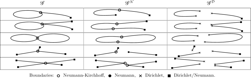
Figure 6: The figure represents the graphs described in the proof of Proposition 2.5. The first column shows the graphs $\mathscr{G}$ considered: tadpole, two-tails tadpole, double-rings graph, star graph with $N=3$ and star graph with $N=4$. The second and the third columns respectively provide the corresponding graphs $\mathscr{G}^{N}$ and $\mathscr{G}^{D}$.

3 Main results

3.1 Abstract controllability result

Let $\eta>0$ and $a\geq 0$. We denote by $I$ the subset of $(\mathbb{N}^{*})^{2}$ such that $I:=\{(j,k)\in(\mathbb{N}^{*})^{2}:j<k\}$.

Assumptions I ($\eta$).

The bounded symmetric operator $B$ satisfies the following conditions.

1. There exists $C>0$ such that $|\langle\phi_{j},B\phi_{1}\rangle_{L^{2}}|\geq\frac{C}{j^{2+\eta}}$ for every $j\in\mathbb{N}^{*}$.

2. For $(j,k),(l,m)\in I$ such that $(j,k)\neq(l,m)$ and such that $\lambda_{j}-\lambda_{k}=\lambda_{l}-\lambda_{m},$ we have

   $$\langle\phi_{j},B\phi_{j}\rangle_{L^{2}}-\langle\phi_{k},B\phi_{k}\rangle_{L^{2}}\neq\langle\phi_{l},B\phi_{l}\rangle_{L^{2}}-\langle\phi_{m},B\phi_{m}\rangle_{L^{2}}.$$

The first condition of Assumptions I quantifies how much $B$ mixes the eigenspaces associated to the eigenfunctions $(\phi_{k})_{k\in\mathbb{N}^{*}}$. This assumption is crucial for the controllability. Indeed, when $B$ stabilizes such spaces, also $\Gamma_{T}^{u}$, the unitary propagator associated to the (BSE), does the same and we can not expect to obtain controllability results. The second hypothesis is used to decouple some eigenvalues resonances appearing in the proof of the approximate controllability that we use in order to prove our main results.

Assumptions II ($\eta,a$).

Let $Ran(B|_{H^{2}_{\mathscr{G}}})\subseteq H^{2}_{\mathscr{G}}$ and one of the following assumptions be satisfied.

1. When $\mathscr{G}$ is equipped with ($\mathcal{D}$/$\mathcal{N}$) and $a+\eta\in(0,3/2)$, there exists $d\in[\max\{a+\eta,1\},3/2)$ such that $Ran(B|_{H_{\mathscr{G}}^{2+d}})\subseteq H^{2+d}\cap H^{2}_{\mathscr{G}}.$

2. When $\mathscr{G}$ is equipped with ($\mathcal{N}$) and $a+\eta\in(0,7/2)$, there exist $d\in[\max\{a+\eta,2\},7/2)$ and $d_{1}\in(d,7/2)$ such that $Ran(B|_{H_{\mathscr{G}}^{2+d}})\subseteq H^{2+d}\cap H^{1+d}_{\mathcal{N}\mathcal{K}}\cap H^{2}_{\mathscr{G}}$ and $Ran(B|_{H^{d_{1}}_{\mathcal{N}\mathcal{K}}})\subseteq H^{d_{1}}_{\mathcal{N}\mathcal{K}}.$

3. When $\mathscr{G}$ is equipped with ($\mathcal{D}$) and $a+\eta\in(0,5/2)$, there exists $d\in[\max\{a+\eta,1\},5/2)$ such that $Ran(B|_{H_{\mathscr{G}}^{2+d}})\subseteq H^{2+d}\cap H^{1+d}_{\mathcal{N}\mathcal{K}}\cap H^{2}_{\mathscr{G}}.$ If $d\geq 2$, then there exists $d_{1}\in(d,5/2)$ such that $Ran(B|_{H^{d_{1}}})\subseteq H^{d_{1}}.$

Assumptions II calibrate the regularity of the control potential $B$ according to the choice of the boundary conditions defining $D(A)$ which affects the definition of the spaces $H^{s}_{\mathscr{G}}=D(|A|^{\frac{s}{2}})$ with $s>0$.

We are finally ready to present our main abstract controllability result for the (BSE) on general networks.

Definition 3.1.

Let $\Gamma_{T}^{u}$ be the unitary propagator associated to (BSE) with $T>0$ and $u\in L^{2}((0,T),\mathbb{R})$. The $(\ref{mainx1})$ is said to be globally exactly controllable in $H^{s}_{\mathscr{G}}$ with $s>0$ when, for every $\psi^{1},\psi^{2}\in H^{s}_{\mathscr{G}}$ such that $\|\psi^{1}\|_{L^{2}}=\|\psi^{2}\|_{L^{2}}$, there exist $T>0$ and $u\in L^{2}((0,T),\mathbb{R})$ such that $\Gamma_{T}^{u}\psi^{1}=\psi^{2}.$

Theorem 3.2.

Let $\mathscr{G}$ be a compact quantum graph. Let $\mathcal{M}\in\mathbb{N}^{*}$ be defined in Lemma 2.4. Let exist $C>0$ and $\tilde{d}\geq 0$ such that

(10) $$|\lambda_{k+1}-\lambda_{k}|\geq Ck^{-\frac{\tilde{d}}{\mathcal{M}-1}},\ \ \ \ \ \ \ \ \forall k\in\mathbb{N}^{*}.$$

If the couple $(A,B)$ satisfies Assumptions I$(\eta)$ and Assumptions II$(\eta,\tilde{d})$ for some $\eta>0$, then the $(\ref{mainx1})$ is globally exactly controllable in $H^{s}_{\mathscr{G}}$ for $s=2+d$ and $d$ from Assumptions II.

Proof.

See Section 5.∎

In the next proposition, we state an abstract global exact controllability result valid when $\mathscr{G}$ is one of the graphs represented in Figure 2. This result leads to Theorem 1.2.

Proposition 3.3.

Let $\{L_{j}\}_{j\leq N}\in\mathcal{A}\mathcal{L}(N)$. Let $\mathscr{G}$ be either a tadpole, a two-tails tadpole, a double-rings graph or a star graph with $N\leq 4$ edges. Let $\mathscr{G}$ be equipped with ($\mathcal{D}$/$\mathcal{N}$). If the couple $(A,B)$ satisfies Assumptions I$(\eta)$ and Assumptions II$(\eta,\epsilon)$ for some $\eta,\epsilon>0$, then the $(\ref{mainx1})$ is globally exactly controllable in $H^{s}_{\mathscr{G}}$ for $s=2+d$ and $d$ from Assumptions II.

Proof.

The claim follows by the validity of the spectral hypothesis of Theorem 3.2 due to Proposition 2.5.∎

Remark 3.4.

Let $\{L_{j}\}_{j\leq 2}\in\mathcal{A}\mathcal{L}(2)$. Proposition 2.5 and then Proposition 3.3 are also valid when $\mathscr{G}$ is a two-tails tadpole with tails of length $L_{2}$ and head $L_{1}$. The same is true when $\mathscr{G}$ is a star graph with $3$ (or $4$) edges such that two edges are long $L_{1}$ and the remaining one (resp. ones) $L_{2}$.

The size of the time in Theorem 3.2 depends on the initial and the final states of the dynamics. This is due to the global approximate controllability result adopted in the proof of Theorem 3.2. Nevertheless, the local exact controllability (presented in Proposition 5.2), is valid for any $T>0$ (see Remark 5.3 for further details).

3.2 Proof of Theorem 1.2

Proof.

Let $\mathscr{G}$ be a star graph with $3$ edges of lengths $\{L_{j}\}_{j\leq 3}$ equipped ($\mathcal{D}$). The ($\mathcal{D}$) conditions on the external vertices imply that each eigenfunction $\phi_{j}$ with $j\in\mathbb{N}^{*}$ satisfies $\phi_{j}^{l}(0)=0$ for every $l\leq 3$. Then,

$$\phi_{j}(x)=\big{(}a^{1}_{j}\sin(x\sqrt{\lambda}_{j}),a_{j}^{2}\sin(x\sqrt{\lambda}_{j}),a_{j}^{3}\sin(x\sqrt{\lambda}_{j})\big{)}$$

with $\{a_{j}^{l}\}_{l\leq 3}\subset\mathbb{C}$ such that $(\phi_{j})_{j\in\mathbb{N}^{*}}$ forms a Hilbert basis of $L^{2}(\mathscr{G},\mathbb{C})$, i.e.

(11) $$\sum_{l\leq 3}\int_{0}^{L_{l}}|a_{j}^{l}|^{2}\sin^{2}(x\sqrt{\lambda}_{j})dx=\sum_{l\leq 3}|a_{j}^{l}|^{2}\Big{(}\frac{L_{l}}{2}+\frac{\cos(L_{l}\sqrt{\lambda}_{j})\sin(L_{l}\sqrt{\lambda}_{j})}{2\sqrt{\lambda}_{j}}\Big{)}=1.$$

For every $j\in\mathbb{N}^{*}$, the ($\mathcal{N}\mathcal{K}$) condition in $V_{i}$ yields

(12) $$\begin{split}a^{1}_{j}\sin(\sqrt{\lambda}_{j}L_{1})=...=a^{3}_{j}\sin(\sqrt{\lambda}_{j}L_{3}),\ \ \ \ \ \ \sum_{l\leq 3}a^{l}_{j}\cos(\sqrt{\lambda}_{j}L_{l})=0,\\ \sum_{l\leq 3}\cot(\sqrt{\lambda}_{j}L_{l})=0,\ \ \ \ \ \ \ \ \ \ \sum_{l\leq 3}|a_{j}^{l}|^{2}{\sin(L_{l}\sqrt{\lambda}_{j})\cos(L_{l}\sqrt{\lambda}_{j})}=0.\\ \end{split}$$

Now, (11) and (12) ensure $1=\sum_{l=1}^{3}|a_{j}^{l}|^{2}{L_{l}}/{2}$. The continuity implies $a_{j}^{l}=a_{j}^{1}\frac{\sin(\sqrt{\lambda}_{j}L_{1})}{\sin(\sqrt{\lambda}_{j}L_{l})}$ for $l\neq 1$ and

(13) $$\begin{split}|a_{j}^{1}|^{2}\Bigg{(}L_{1}+\sum_{l=2}^{3}L_{l}\frac{\sin^{2}(\sqrt{\lambda}_{j}L_{1})}{\sin^{2}(\sqrt{\lambda}_{j}L_{l})}\Bigg{)}={2},\ \ \ \ \ \ \ \Longrightarrow\ \ \ \ \ \ |a_{j}^{1}|^{2}&=\frac{2\prod_{m\neq 1}\sin^{2}(\sqrt{\lambda}_{j}L_{m})}{\sum_{k=1}^{3}L_{k}\prod_{m\neq k}\sin^{2}(\sqrt{\lambda}_{j}L_{m})}.\end{split}$$

From $(\ref{tremor})$ and $(\ref{pistola})$, we have $\sum_{l=1}^{3}\cos(\sqrt{\lambda}_{k}L_{l})\prod_{m\neq l}\sin(\sqrt{\lambda}_{k}L_{m})=0$. The validity of [DZ06, Proposition A.11] and Lemma 2.3 ensure that, for every $\epsilon>0$, there exist $C_{1},C_{2}>0$ such that, for every $j\in\mathbb{N}^{*}$,

(14) $$\begin{split}|a_{j}^{1}|&=\sqrt{\frac{2}{\sum_{l=1}^{3}L_{l}\sin^{-2}(\sqrt{\lambda}_{j}L_{l})}}\geq\sqrt{\frac{2}{\sum_{l=1}^{3}L_{l}C_{1}^{-2}{\lambda_{j}^{1+\epsilon}}}}\geq\frac{C_{2}}{j^{1+\epsilon}}.\\ \end{split}$$

1) Validation of Assumptions I.1 . We notice $\langle\phi_{k}^{l},(B\phi_{j})^{l}\rangle_{L^{2}(e_{j},\mathbb{C})}=0$ for $l\neq 1$ and $k,j\in\mathbb{N}^{*}$. Let

$$a_{j}(x):=\frac{2\prod_{m\neq 1}\sin^{2}(\sqrt{\lambda_{j}}L_{m})}{\sum_{k=2}^{4}L_{k}\sin^{2}(\sqrt{\lambda_{j}}x)\prod_{{m\neq k,1}}\sin^{2}(\sqrt{\lambda_{j}}L_{m})+x\prod_{{m\neq 1}}\sin^{2}(\sqrt{\lambda_{j}}L_{m})},$$

$$B_{1}(x):=\frac{-30\sqrt{\lambda_{1}}x+20\sqrt{\lambda_{1}}^{3}x^{3}+4\sqrt{\lambda_{1}}^{5}x^{5}+15\sin(2\sqrt{\lambda_{1}}x)}{40\sqrt{\lambda_{1}}^{5}},$$

$$\begin{split}B_{j}(x)&:=2\frac{-6(\sqrt{\lambda_{1}}-\sqrt{\lambda_{j}})x+(\sqrt{\lambda_{1}}-\sqrt{\lambda_{j}})^{3}x^{3}+6\sin((\sqrt{\lambda_{1}}-\sqrt{\lambda_{j}})x)}{(\sqrt{\lambda_{1}}-\sqrt{\lambda_{j}})^{5}}\\ &-2\frac{-6(\sqrt{\lambda_{1}}+\sqrt{\lambda_{j}})x+(\sqrt{\lambda_{1}}+\sqrt{\lambda_{j}})^{3}x^{3}+6\sin((\sqrt{\lambda_{1}}+\sqrt{\lambda_{j}})x)}{(\sqrt{\lambda_{1}}+\sqrt{\lambda_{j}})^{5}}\\ \end{split}$$

with $j\in\mathbb{N}^{*}$. Each function $\widetilde{B}_{j}(\cdot):=\sqrt{a_{1}(\cdot)}\sqrt{a_{j}(\cdot)}B_{j}(\cdot)$ is non-constant and analytic in $\mathbb{R}^{+}$, while we notice that $B_{1,j}=\langle\phi_{1},B\phi_{j}\rangle_{L^{2}}=\widetilde{B}_{j}(L_{1})$ by calculation. The set of positive zeros $\tilde{V}_{j}$ of each $\widetilde{B}_{j}$ is a discrete subset of $\mathbb{R}^{+}$ and $\tilde{V}=\bigcup_{j\in\mathbb{N}^{*}}\tilde{V}_{j}$ is countable. For every $\{L_{l}\}_{l\leq 4}\in\mathcal{A}\mathcal{L}(4)$ such that $L_{1}\not\in\tilde{V}$, we have $|B_{1,j}|\neq 0$ for every $j\in\mathbb{N}^{*}$. Now, there holds $|B_{1,j}|\sim{|a_{j}|L_{1}\sqrt{\lambda_{1}}\sqrt{\lambda_{j}}}{(\lambda_{j}-\lambda_{1})^{-2}}$ for every $j\in\mathbb{N}^{*}\setminus\{1\}.$ From Lemma 2.3 and the identity $(\ref{oip})$, the first point of Assumptions I($2+\epsilon$) is verified as, for each $\epsilon>0$, there exists $C_{3}>0$ such that

$$|B_{1,j}|\geq\frac{C_{3}}{j^{4+\epsilon}},\ \ \ \ \ \forall j\in\mathbb{N}^{*}.$$

2) Validation of Assumptions I.2 . By calculation, we notice that $B_{j,j}=\langle\phi_{j},B\phi_{j}\rangle_{L^{2}}=F_{j}(L_{1})$ where

$$\begin{split}F_{j}(x)&:=a_{j}(x)\frac{-30\sqrt{\lambda}_{k}x+20\sqrt{\lambda}_{k}^{3}x^{3}+4\sqrt{\lambda}_{k}^{5}x^{5}+15\sin(2\sqrt{\lambda}_{k}x)}{40\sqrt{\lambda}_{k}^{5}}.\\ \end{split}$$

Let $(k,j),(m,n)\in I,\ (k,j)\neq(m,n)$ for $I$ defined above Assumptions I. For $F_{j,k,l,m}(x)=F_{j}(x)-F_{k}(x)-F_{l}(x)+F_{m}(x),$ it follows $F_{j,k,l,m}(L_{1})=B_{j,j}-B_{k,k}-B_{l,l}+B_{m,m}$ and $F_{j,k,l,m}(x)$ is a non-constant analytic function for $x>0$. Furthermore $V_{j,k,l,m}$, the set of the positive zeros of $F_{j,k,l,m}(x)$, is discrete and $V:=\bigcup_{\underset{j\neq k\neq l\neq m}{j,k,l,m\in\mathbb{N}^{*}}}V_{j,k,l,m}$ is a countable subset of $\mathbb{R}^{+}$. For each $\{L_{l}\}_{l\leq 3}\in\mathcal{A}\mathcal{L}(3)$ such that $L_{1}\not\in V\cup\tilde{V}$, Assumptions I$(2+\epsilon)$ are verified.

3) Validation of Assumptions II.3 and conclusion. We notice that $B$ stabilizes the spaces $H^{2}_{\mathscr{G}}$, $H^{m}$ and $H^{m}_{\mathcal{N}\mathcal{K}}$ for $m\in(0,9/2)$ since, for $n\in\mathbb{N}^{*}$ such that $n<5$, we have

$$\partial_{x}^{n-1}(B\psi)^{1}(L_{1})=....=\partial_{x}^{n-1}(B\psi)^{3}(L_{3})=0,\ \ \ \ \ \ \forall\psi\in H^{n}_{\mathcal{N}\mathcal{K}},$$

which implies $B\psi\in H^{n}_{\mathcal{N}\mathcal{K}}.$ The third point of Assumptions II($2+\epsilon_{1},\epsilon_{2}$) is valid for each $\epsilon_{1},\epsilon_{2}>0$ such that $\epsilon_{1}+\epsilon_{2}\in(0,1/2)$. From Proposition 3.3, the controllability holds in $H_{\mathscr{G}}^{4+\epsilon}$ with $\epsilon>0$. Finally, we note that $H_{\mathscr{G}}^{4+\epsilon}=H^{4+\epsilon}\cap H^{4}_{\mathscr{G}}$ (see Proposition 4.2 for further details).∎

Remark 3.5.

The proof Theorem 1.2 can also be adapted for star-graphs equipped with ($\mathcal{N}$) or with ($\mathcal{D}/\mathcal{N}$). In such cases, we respectively have to use Proposition A.2 and Remark A.3 instead of [DZ06, Proposition A.11].

Remark 3.6.

Let us consider a three edges star graph $\mathscr{G}$ equipped with ($\mathcal{D}$). The same observations can be done for star graphs of $N\in\mathbb{N}^{*}$ edges and equipped with ($\mathcal{D}$/$\mathcal{N}$)

1) When $\{L_{1},L_{2},L_{3}\}\in\mathcal{A}\mathcal{L}(3)$, each eigenfuction $\phi=(\phi^{1},\phi^{2},\phi^{3})$ of $A$ is such that $\phi^{j}\not\equiv 0$ for every $j\leq 3$. Indeed, if for instance $\phi^{1}\equiv 0$, then the continuity would imply $\phi^{2}(L_{2})=\phi^{3}(L_{3})=0$ and then the corresponding eigenvalue $\lambda$ would be the form $\lambda=\frac{n_{1}^{2}\pi^{2}}{L_{2}^{2}}$ and $\lambda=\frac{n_{2}^{2}\pi^{2}}{L_{3}^{2}}$ for suitable $n_{1},n_{2}\in\mathbb{N}^{*}$ which is impossible.

2) When $L_{2}/L_{3}$ is rational, there exist $n,m\in\mathbb{N}^{*}$ such that ${L_{2}}/{L_{3}}={n}/{m}$. In this case, there exist eigenfuctions of $A$ of the form $(0,\sin(\sqrt{\mu}x),-\sin(\sqrt{\mu}x))$ where $\mu=\frac{k^{2}m^{2}\pi^{2}}{L_{3}^{2}}$ is the corresponding eigenvalue for some $k\in\mathbb{N}^{*}$. When also $L_{1}/L_{3}$ is rational, there exist $n^{\prime},m^{\prime},\in\mathbb{N}^{*}$ such that ${L_{1}}/{L_{3}}={n^{\prime}}/{m^{\prime}}.$ The sequence $\{\mu_{k}\}_{k\in\mathbb{N}^{*}}$ with $\mu_{k}=\frac{k^{2}m^{2}m^{\prime 2}\pi^{2}}{L_{3}^{2}}$ is composed by eigenvalues of $A$ and they are multiple. Indeed, fixed $k\in\mathbb{N}^{*}$,

$$f_{k}=\big{(}-2\sin(\sqrt{\mu}_{k}x),\sin(\sqrt{\mu}_{k}x),\sin(\sqrt{\mu}_{k}x)\big{)},\ \ \ \ \ \ \ \ g_{k}=\big{(}0,\sin(\sqrt{\mu}_{k}x),-\sin(\sqrt{\mu}_{k}x)\big{)}$$

are reciprocally orthogonal eigenfunctions of $A$ corresponding to $\mu_{k}$.

3.3 Controllability of a bilinear quantum system on a tadpole graph

Another application of Theorem 3.2 is the following. Let $\mathscr{G}$ be a tadpole graph composed by two edges $\{e_{1},e_{2}\}$ connected in an internal vertex $v$. The edge $e_{1}$ is self-closing and parametrized in the clockwise direction with a coordinate going from $0$ to $L_{1}$ (the length $e_{1}$). On the “tail” $e_{2}$, we consider a coordinate going from $0$ in the to $L_{2}$ and we associate the $0$ to the external vertex $\tilde{v}$.

Figure 7: The parametrization of the tadpole graph and its symmetry axis $r$.

Theorem 3.7.

Let $\mathscr{G}$ be a tadpole graph equipped with ($\mathcal{D}$). Let $B:\psi\in L^{2}(\mathscr{G},\mathbb{C})\longrightarrow(\mu_{1}\psi^{1},\mu_{2}\psi^{2})$ with

$$\mu_{1}(x):=\sin\big{(}\frac{2\pi}{L_{1}}x\big{)}+x(x-L_{1}),\ \ \ \ \ \mu_{2}(x):=x^{2}-(2L_{1}+2L_{2})x+L_{2}^{2}+2L_{1}L_{2}.$$

There exists $\mathcal{C}\subset(\mathbb{R}^{+})^{2}$ countable so that, for each $\{L_{1},L_{2}\}\in\mathcal{A}\mathcal{L}(2)\setminus\mathcal{C}$, the $(\ref{mainx1})$ is globally exactly controllable in $H^{4+\epsilon}_{\mathscr{G}}$ with $\epsilon>0$.

Proof.

Let $r$ be the symmetry axis of $\mathscr{G}$ (see Figure 7). We construct $(\phi_{k})_{k\in\mathbb{N}^{*}}$ as a sequence of symmetric or skew-symmetric functions with respect to $r$. If $\phi_{k}=(\phi_{k}^{1},\phi_{k}^{2})$ is skew-symmetric, then $\phi^{2}_{k}\equiv 0$, $\phi^{1}_{k}(0)=\phi^{1}_{k}(L_{1}/2)=\phi^{1}_{k}(L_{1})=0$ and $\partial_{x}\phi^{1}_{k}(0)=\partial_{x}\phi^{1}_{k}(L_{1}).$ We respectively denote by

$$(f_{k})_{k\in\mathbb{N}^{*}}=\left(\Big{(}\sqrt{\frac{2}{L_{1}}}\sin\Big{(}x\frac{2k\pi}{L_{1}}\Big{)},0\Big{)}\right)_{k\in\mathbb{N}^{*}},\ \ \ \ \ \ (\nu_{k})_{k\in\mathbb{N}^{*}}:=\left(\frac{4k^{2}\pi^{2}}{L_{1}^{2}}\right)_{k\in\mathbb{N}^{*}}$$

the skew-symmetric eigenfunctions belonging to the Hilbert base $(\phi_{k})_{k\in\mathbb{N}^{*}}$ and the ordered sequence of corresponding eigenvalues. If $\phi_{k}=(\phi_{k}^{1},\phi_{k}^{2})$ is symmetric, then we have $\partial_{x}\phi^{1}_{k}(L_{1}/2)=0$ and $\phi_{k}^{1}(\cdot)=\phi_{k}^{1}(L_{1}-\cdot)$. The ($\mathcal{D}$) conditions on $\widetilde{v}$ implies that the symmetric eigenfunctions corresponding to the eigenvalues $(\mu_{k})_{k\in\mathbb{N}^{*}}$ are

$$(g_{k})_{k\in\mathbb{N}^{*}}:=\Big{(}\Big{(}a_{k}^{1}\cos\Big{(}\sqrt{\mu_{k}}\Big{(}x-\frac{L_{1}}{2}\Big{)}\Big{)},a_{k}^{2}\sin(\sqrt{\mu_{k}}x)\Big{)}\Big{)}_{k\in\mathbb{N}^{*}},\ \ \ \ \ \text{for}\ \ \ \ \ \{(a_{k}^{1},a_{k}^{2})\}_{k\in\mathbb{N}^{*}}\subset\mathbb{C}^{2}.$$

Now, we characterize the eigenvalues $(\mu_{k})_{k\in\mathbb{N}^{*}}$. The $(\mathcal{N}\mathcal{K})$ conditions in $v$ ensure that $a_{k}^{1}\cos(\sqrt{\mu_{k}}(L_{1}/2))=a_{k}^{2}\sin(\sqrt{\mu_{k}}L_{2}))$ and $2a_{k}^{1}\sin(\sqrt{\mu_{k}}(L_{1}/2))+a_{k}^{2}\cos(\sqrt{\mu_{k}}L_{2}))=0$. Finally, $(\mu_{k})_{k\in\mathbb{N}^{*}}$ are the zeros of

(15) $$2\tan(\sqrt{\mu_{k}}(L_{1}/2))+\cot(\sqrt{\mu_{k}}L_{2}))=0.$$

The remaining part of the proof follows by the same argument of the one of Theorem 1.2. The only difference is that we need to use Remark A.3 instead of [DZ06, Proposition A.11]. ∎

Remark 3.8.

As showed in the proof of Theorem 1.2, the study of the spectrum of $A$ on a $3$-edges star-graph equipped with ($\mathcal{D}$) consists in seeking for $(\lambda_{k})_{k\in\mathbb{N}}$ solving the first two identities of (12). If for instance the lengths of the edges are equal to $L>0$, the eigenvalues are the zeros of $\sin(\sqrt{\lambda}L)$ and of $\cos(\sqrt{\lambda}L)$. However, in the general framework, the eigenvalues are obtained by solving $\sum_{l\leq 3}\cot(\sqrt{\lambda}L_{l})=0$ which is a transcendental equation and then not always explicitly solvable. Similarly in Theorem 3.7, some eigenvalues are the zeros of the transcendental equation (15). The same observations is valid for other graphs (see [DZ06] for further details).

4 Well-posedness and interpolation properties of the spaces $H^{s}_{\mathscr{G}}$

In the current section, we provide the well-posedness of the $(\ref{mainx1})$.

Theorem 4.1.

Let $(A,B)$ satisfy Assumptions II$(\eta,\tilde{d})$ with $\eta>0$ and $\tilde{d}\geq 0$. Let $\psi^{0}\in H^{2+d}_{\mathscr{G}}$ with $d$ introduced in Assumptions II. Let $u\in L^{2}((0,T),\mathbb{R})$ with $T>0$. There exists a unique mild solution of (BSE) in $H^{2+d}_{\mathscr{G}}$, i.e. a function $\psi\in C_{0}([0,T],H^{2+d}_{\mathscr{G}})$ such that for every $t\in[0,T]$,

(16) $$\psi(t,x)=e^{-iAt}\psi^{0}(x)-i\int_{0}^{t}e^{-iA(t-s)}u(s)\psi(s,x)ds.$$

Moreover, there exists $C=C(T,B,u)>0$ so that $\|\psi\|_{C^{0}([0,T],H^{2+d}_{\mathscr{G}})}\leq C\|\psi^{0}\|_{H^{2+d}_{\mathscr{G}}}$, while $\|\psi(t)\|_{L^{2}}=\|\psi^{0}\|_{L^{2}}$ for every $t\in[0,T]$ and $\psi_{0}\in H^{2+d}_{\mathscr{G}}.$

Before proving Theorem 4.1, we present some interpolation properties for the spaces $H^{s}_{\mathscr{G}}$ with $s\geq 0$ in the following proposition. In this result, we denote by $H^{0}_{\mathscr{G}},\ H^{0}_{\mathcal{N}\mathcal{K}}$ and $H^{0}$ the Hilbert space $L^{2}(\mathscr{G},\mathbb{C})$.

Proposition 4.2.

1) If the compact quantum graph $\mathscr{G}$ is equipped with ($\mathcal{D}$/$\mathcal{N}$), then

$$H^{s_{1}+s_{2}}_{\mathscr{G}}=H_{\mathscr{G}}^{s_{1}}\cap H^{s_{1}+s_{2}}\ \ \ \text{for}\ \ \ s_{1}\in\mathbb{N},\ s_{2}\in[0,1/2).$$

2) If the compact quantum graph $\mathscr{G}$ is equipped with ($\mathcal{N}$), then

$$H^{s_{1}+s_{2}}_{\mathscr{G}}=H_{\mathscr{G}}^{s_{1}}\cap H^{s_{1}+s_{2}}_{\mathcal{N}\mathcal{K}}\ \ \ \text{for}\ \ \ s_{1}\in 2\mathbb{N},\ s_{2}\in[0,3/2).$$

3) If the compact quantum graph $\mathscr{G}$ is equipped with ($\mathcal{D}$), then

$$H^{s_{1}+s_{2}+1}_{\mathscr{G}}=H_{\mathscr{G}}^{s_{1}+1}\cap H^{s_{1}+s_{2}+1}_{\mathcal{N}\mathcal{K}}\ \ \ \text{for}\ \ \ s_{1}\in 2\mathbb{N},\ s_{2}\in[0,3/2).$$

Proof.

1) Graph equipped with ($\mathcal{D}$/$\mathcal{N}$). We start by proving the first statement of Proposition 4.2.

1) (a) Preliminaries. Let $I^{\mathcal{N}}$ and $I^{\mathcal{D}}$ be two quantum graphs defined on an interval $I$ of length $L$. We suppose that $I^{\mathcal{N}}$ is equipped with $(\mathcal{N})$, while $I^{\mathcal{D}}$ is equipped with $(\mathcal{D})$. From [Gru16, Definition  2.1], for every $s_{1}\in 2\mathbb{N},$ $s_{2}\in[0,3/2)$ and $s_{3}\in[0,1/2)$, we have

(17) $$\begin{split}H^{s_{1}+s_{2}}_{I^{\mathcal{N}}}=H_{I^{\mathcal{N}}}^{s_{1}}\cap H^{s_{1}+s_{2}}(I^{\mathcal{N}},\mathbb{C}),\ \ \ H^{s_{1}+s_{2}+1}_{I^{\mathcal{D}}}=H_{I^{\mathcal{D}}}^{s_{1}+1}\cap H^{s_{1}+s_{2}+1}(I^{\mathcal{D}},\mathbb{C}),\ \ \ H^{s_{3}}_{I^{\mathcal{D}}}=H^{s_{3}}(I^{\mathcal{D}},\mathbb{C}).\\ \end{split}$$

Let $\mathscr{G}=I^{\mathcal{M}}$ be an interval equipped with $(\mathcal{N})$ in the external vertex parametrized with $0$ and with ($\mathcal{D}$) in the other. We prove

(18) $$H^{s_{1}+s_{2}}_{I^{\mathcal{M}}}=H_{I^{\mathcal{M}}}^{s_{1}}\cap H^{s_{1}+s_{2}}(I^{\mathcal{M}},\mathbb{C}),\ \ \ \ \ \ \forall s_{1}\in\mathbb{N},\ s_{2}\in[0,1/2).\\$$

Let $\widetilde{I}^{\mathcal{D}}$ and $\widetilde{I}^{\mathcal{N}}$ respectively be two sub-intervals of ${I}^{\mathcal{M}}$ of length $\frac{3}{4}L$. The interval $\widetilde{I}^{\mathcal{D}}$ contains one external vertex of ${I}^{\mathcal{M}}$, while $\widetilde{I}^{\mathcal{N}}$ contains the other. We consider both the intervals as quantum graphs: $\widetilde{I}^{\mathcal{D}}$ is equipped in both the external vertices with $(\mathcal{D})$ and $\widetilde{I}^{\mathcal{N}}$ is equipped with $(\mathcal{N})$. Fixed $s>0$,

$$H^{s}(I^{\mathcal{M}},\mathbb{C})=H^{s}({\widetilde{I}^{\mathcal{D}}},\mathbb{C})\times H^{s}({\widetilde{I}^{\mathcal{N}}},\mathbb{C}),\ \ \ \ \ \ \ \ \ L^{2}(I^{\mathcal{M}},\mathbb{C})=L^{2}({\widetilde{I}^{\mathcal{D}}},\mathbb{C})\ \times\ L^{2}({\widetilde{I}^{\mathcal{N}}},\mathbb{C}).$$

Let $[\cdot,\cdot]_{\theta}$ be the complex interpolation of spaces for $0<\theta<1$ defined in [Tri95,  Definition, Chapter 1.9.2]. From [Tri95,  Chapter 1.15.1 & Chapter 1.15.3], for $s_{2}\in[0,1/2)$, we have $\big{[}L^{2}(\widetilde{I}^{\mathcal{N}},\mathbb{C}),H^{2}_{\widetilde{I}^{\mathcal{N}}}\big{]}_{s_{2}/2}=H^{s_{2}}_{\widetilde{I}^{\mathcal{N}}}$ and $\big{[}L^{2}(\widetilde{I}^{\mathcal{D}},\mathbb{C}),H^{2}_{\widetilde{I}^{\mathcal{D}}}\big{]}_{s_{2}/2}=H^{s_{2}}_{\widetilde{I}^{\mathcal{D}}}.$ Thanks to [Tri95,  relation (12), Chapter 1.18.1], we have

$$\Big{[}L^{2}(\widetilde{I}^{\mathcal{N}},\mathbb{C})\ \times\ L^{2}(\widetilde{I}^{\mathcal{D}},\mathbb{C}),H^{2}_{\widetilde{I}^{\mathcal{N}}}\ \times\ H^{2}_{\widetilde{I}^{\mathcal{D}}}\Big{]}_{{s_{2}}/2}=\Big{[}L^{2}(\widetilde{I}^{\mathcal{N}},\mathbb{C}),H^{2}_{\widetilde{I}^{\mathcal{N}}}\Big{]}_{{s_{2}}/2}\ \times\ \Big{[}L^{2}(\widetilde{I}^{\mathcal{D}},\mathbb{C}),H^{2}_{\widetilde{I}^{\mathcal{D}}}\Big{]}_{{s_{2}}/2},$$

$$\begin{split}&\Longrightarrow\ \ \ \ H^{s_{2}}_{I^{\mathcal{M}}}=\Big{[}L^{2}(I^{\mathcal{M}},\mathbb{C}),H^{2}_{I^{\mathcal{M}}}\Big{]}_{{s_{2}}/2}=\Big{[}L^{2}(\widetilde{I}^{\mathcal{N}},\mathbb{C}),H^{2}_{\widetilde{I}^{\mathcal{N}}}\Big{]}_{{s_{2}}/2}\ \times\ \Big{[}L^{2}(\widetilde{I}^{\mathcal{D}},\mathbb{C}),H^{2}_{\widetilde{I}^{\mathcal{D}}}\Big{]}_{{s_{2}}/2}=H^{s_{2}}_{\widetilde{I}^{\mathcal{N}}}\ \times\ H^{s_{2}}_{\widetilde{I}^{\mathcal{D}}}.\end{split}$$

Equivalently, $H^{s_{1}+s_{2}}_{I^{\mathcal{M}}}=H^{s_{1}+s_{2}}_{\widetilde{I}^{\mathcal{N}}}\times H^{s_{1}+s_{2}}_{\widetilde{I}^{\mathcal{D}}}$ for every $s_{1}\in\mathbb{N}^{*}$ and $s_{2}\in[0,1/2)$ which leads to $(\ref{chenon2})$ thanks to $(\ref{chenon})$.

1) (b) Sobolev’s spaces for star graphs with equal edges. Let $I^{\mathcal{N}}$ and $I^{\mathcal{M}}$ be defined as in 1) (a). We respectively call $A_{\mathcal{N}}$ and $A_{\mathcal{M}}$ the two self-adjoint Laplacians defining $I^{\mathcal{N}}$ and $I^{\mathcal{M}}$. Let $(f_{j}^{1})_{j\in\mathbb{N}^{*}}$ be a Hilbert basis of $L^{2}(I,\mathbb{C})$ made by eigenfunctions of $A_{\mathcal{N}}$ and $(f_{j}^{2})_{j\in\mathbb{N}^{*}}$ a Hilbert basis of $L^{2}(I,\mathbb{C})$ composed by eigenfunctions of $A_{\mathcal{M}}$. Let $\mathscr{G}$ be a star graph of $N$ edges long $L$ and equipped with ($\mathcal{N}$). The ($\mathcal{N}$) conditions on $V_{e}$ imply that

$$\phi_{k}=(a^{1}_{k}\cos(x\sqrt{\lambda}_{k}),...,a_{j}^{N}\cos(x\sqrt{\lambda}_{k})),\ \ \ \ \forall k\in\mathbb{N}^{*}$$

where $\lambda_{k}$ is the corresponding eigenvalue and for suitable $\{a_{k}^{l}\}_{l\leq N}\subset\mathbb{C}$. The ($\mathcal{N}\mathcal{K}$) condition in $V_{i}$ ensures that

$$\sin(\sqrt{\lambda}_{k}L)\sum_{l\leq N}a^{l}_{k}=0,\ \ \ \ \ \ \ \ a^{1}_{k}\cos(\sqrt{\lambda}_{k}L)=...=a^{N}_{k}\cos(\sqrt{\lambda}_{k}L),\ \ \ \ \ \forall k\in\mathbb{N}^{*}.$$

Thus, each eigenvalue is either of the form $\frac{(n-1)^{2}\pi^{2}}{L^{2}}$ when $\sum_{l\leq N}a^{l}_{k}\neq 0$, or $\frac{(2n-1)^{2}\pi^{2}}{4L^{2}}$ when $\sum_{l\leq N}a^{l}_{k}=0$ for suitable $n\in\mathbb{N}^{*}$. For every $k\in\mathbb{N}^{*}$, there exists $j(k)\in\mathbb{N}^{*}$ such that

(19) $$\begin{split}\phi_{k}^{l}\ \ \ \text{ is equal either to }\ \ \ c_{k}^{l}f^{1}_{j(k)},\ \ \ \text{ or to }\ \ \ c_{k}^{l}f^{2}_{j(k)}\ \ \ \text{ with }\ \ \ c_{k}^{l}\in\mathbb{C},\ \ |c_{k}^{l}|\leq 1,\ \ \ \forall l\in\{1,...,N\}.\\ \end{split}$$

In addition, for each $k\in\mathbb{N}^{*}$ and $m\in\{1,2\}$, there exist $\widetilde{j}(k)\in\mathbb{N}^{*}$ and $l\leq N$ such that $f^{m}_{k}=c_{\widetilde{j}(k)}^{l}\phi_{\widetilde{j}(k)}^{l}$ with $c_{\widetilde{j}(k)}^{l}\in\mathbb{C}$ uniformly bounded in $k\in\mathbb{N}^{*}$ and $l\leq N$. The last identity and $(\ref{iu})$ tell that the components of the elements $(\phi_{k})_{k\in\mathbb{N}^{*}}$ are elements of $(f_{j}^{1})_{j\in\mathbb{N}^{*}}$ and $(f_{j}^{2})_{j\in\mathbb{N}^{*}}$ and vice versa. Thus, $\psi=(\psi^{1},...,\psi^{N})\in H^{s}_{\mathscr{G}}$ if and only if $\psi^{l}\in H^{s}_{I^{\mathcal{N}}}\cap H^{s}_{I^{\mathcal{M}}}$ for every $l\leq N.$

1) (c) Conclusion. Let $\mathscr{G}$ be equipped with ($\mathcal{D}$/$\mathcal{N}$) and $\widetilde{L}<\min\{L_{k}/2:k\in\{1,...,N\}\}$. Let $n(v)$ be defined in $(\ref{molteplicit})$ for every $v\in V_{e}\cup V_{i}$. We define the graphs $\widetilde{\mathscr{G}}(v)$ for every $v\in V_{i}\cup V_{e}$ and the intervals $\{I_{j}\}_{j\leq N}$ as follows (see Figure 8 for an explicit example). If $v\in V_{i}$, then $\widetilde{\mathscr{G}}(v)$ is a star sub-graph of $\mathscr{G}$ equipped with ($\mathcal{N}$) and composed by $n(v)$ edges long $\widetilde{L}$ and connected to the internal vertex $v$. If $v\in V_{e}$, then $\widetilde{\mathscr{G}}(v)$ is an interval long $\widetilde{L}$ such that the external vertex $v$ is equipped with the same boundary conditions that $v$ has in $\mathscr{G}$. We impose $(\mathcal{N})$ on the other vertex. Let $v,\hat{v}\in V_{e}\cup V_{i}$ be such that $v,\hat{v}\in{e_{1}}.$ Now, the graphs $\widetilde{\mathscr{G}}(v)$ and $\widetilde{\mathscr{G}}(\hat{v})$ have respectively two external vertices $w_{1}$ and $w_{2}$ lying on the same edge $e_{1}$ and such that $w_{1}\not\in\widetilde{\mathscr{G}}(\hat{v})$. We construct an interval $I_{1}$ strictly containing $w_{1}$ and $w_{2}$, strictly contained in $e_{1}$ and equipped with ($\mathcal{N}$). We repeat the procedure for every edge $e_{j}$ with $j\leq N$ and we define the intervals $\{I_{j}\}_{j\leq N}$.

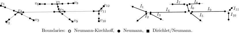
Figure 8: The left and the right figures respectively represent the graphs $\{\widetilde{\mathscr{G}}(v)\}_{v\in V_{i}\cup V_{e}}$ and the intervals $\{I_{j}\}_{j\leq N}$ for a given graph $\mathscr{G}$.

From 1) (a) and 1) (b), for every $v\in V_{i}\cup V_{e}$, $j\leq N$, $s_{1}\in\mathbb{N}$ and $s_{2}\in[0,1/2)$, we have the validity of the identities $H^{s_{1}+s_{2}}_{\widetilde{\mathscr{G}}(v)}=H_{\widetilde{\mathscr{G}}(v)}^{s_{1}}\cap H^{s_{1}+s_{2}}(\widetilde{\mathscr{G}}(v),\mathbb{C})$ and $H^{s_{1}+s_{2}}_{I_{j}}=H_{I_{j}}^{s_{1}}\cap H^{s_{1}+s_{2}}(I_{j},\mathbb{C}).$ We notice that $G:=\{\widetilde{\mathscr{G}}(v_{j})\}_{j\leq M}\cup\{I_{j}\}_{j\leq N}$ covers $\mathscr{G}$. As in 1) (a), we see each function of domain $\mathscr{G}$ as a vector of functions of domain $G_{j}$ with $j\leq M+N$. The first relation of Proposition 4.2 is proved by adopting [Tri95, relation (12), Chapter 1.18.1] as in 1) (a).

2) Graphs equipped with ($\mathcal{N}$). Let $\mathscr{G}$ be equipped with ($\mathcal{N}$) and $N_{e}=|V_{e}|$. We consider $\{\widetilde{\mathscr{G}}(v)\}_{v\in V_{e}}$ introduced in 1) (c) and we define $\widetilde{\mathscr{G}}$ from $\mathscr{G}$ as follows (see Figure 9). For every $v\in V_{e}$, we remove from the edge including $v$, a section of length $\widetilde{L}/2$ containing $v$. We equip the new external vertex with ($\mathcal{N}$).

Figure 9: The left and the right figures respectively represent the graphs $\{\widetilde{\mathscr{G}}(v)\}_{v\in V_{e}}$ and $\widetilde{\mathscr{G}}$ for a given graph $\mathscr{G}$.

We call $G^{\prime}:=\{G^{\prime}_{j}\}_{j\leq N_{e}+1}:=\{\widetilde{\mathscr{G}}(v)\}_{v\in V_{e}}\cup\{\widetilde{\mathscr{G}}\}$ which covers $\mathscr{G}$. For every $s_{1}\in 2\mathbb{N},\ s_{2}\in[0,3/2)$, we have $H^{s_{1}+s_{2}}_{\widetilde{\mathscr{G}}(v)}=H_{\widetilde{\mathscr{G}}(v)}^{s_{1}}\cap H^{s_{1}+s_{2}}$ from $(\ref{chenon})$. Now, $H^{s_{1}+s_{2}}_{\mathcal{N}\mathcal{K}}=H^{s_{1}+s_{2}}_{\widetilde{\mathscr{G}}}\ \times\prod_{v\in V_{e}}H^{s_{1}+s_{2}}(\widetilde{\mathscr{G}}(v),\mathbb{C})$. The second relation of Proposition 4.2 follows from the arguments of 1) (a).

3) Graphs equipped with ($\mathcal{D}$). The third point of Proposition 4.2 is proved as the second by considering $\{\widetilde{\mathscr{G}}(v)\}_{v\in V_{e}}$ as intervals equipped with $(\mathcal{D})$ and $\widetilde{\mathscr{G}}$ equipped with $(\mathcal{D})$ in its external vertices.∎

We are finally ready to prove Theorem 4.1 which follows from Proposition 4.2 and from the following auxiliary result.

Lemma 4.3.

Let $(\lambda_{k})_{k\in\mathbb{N}*}$ be the eigenvalues of a self-adjoint Laplacian $A$ defined on a compact quantum graph equipped with ($\mathcal{D}$), ($\mathcal{N}$) or ($\mathcal{D}/\mathcal{N}$). For every $T>0$, there exists $C(T)>0$ uniformly bounded for $T$ lying on bounded intervals such that

$$\forall g\in L^{2}((0,T),\mathbb{C}),\ \ \ \ \ \ \ \left\|\int_{0}^{T}e^{i\lambda_{(\cdot)}s}g(s)ds\right\|_{\ell^{2}}\leq C(T)\|g\|_{L^{2}((0,T),\mathbb{C})}.$$

Proof.

The result is a consequence of Proposition B.6 which validity is ensured by Lemma 2.4.∎

Proof of Theorem 4.1.

1) Preliminaries. Let $T>0$ and the function $f$ be such that $f(s)\in H^{2+d}\cap H^{1+d}_{\mathcal{N}\mathcal{K}}\cap H^{2}_{\mathscr{G}}$ for almost every $s\in(0,T)$. We introduce

$$G(\cdot):=\int_{0}^{(\cdot)}e^{iA\tau}f(\tau)d\tau.$$

In the first part of the proof, we prove that $G\in C^{0}([0,T],H^{2+d}_{\mathscr{G}})$ by ensuring the existence of $C(T)>0$ uniformly bounded for $T$ lying on bounded intervals such that $\|G\|_{L^{\infty}((0,T),H^{2+d}_{\mathscr{G}})}\leq C(T)\|f\|_{L^{2}((0,T),H^{2+d})}.$ To the purpose, we distinguish the different frameworks described by Assumptions II.

1) (a) Under Assumptions II.1 . Let $f(s)\in H^{3}\cap H_{\mathscr{G}}^{2}$ for almost every $s\in(0,T)$ and $f(s)=(f^{1}(s),...,f^{N}(s))$. We prove that $G\in C^{0}([0,T],H^{3}_{\mathscr{G}})$. Let $t\in(0,T)$. The definition of $G(t)$ implies

(20) $$\begin{split}G(t)=\sum_{k=1}^{\infty}\phi_{k}\int_{0}^{t}e^{i\lambda_{k}s}\langle\phi_{k},f(s)\rangle_{L^{2}}ds,\ \ \ \ \ \ \ \ \ \|G(t)\|_{(3)}=\Big{(}\sum_{k\in\mathbb{N}^{*}}\Big{|}k^{3}\int_{0}^{t}e^{i\lambda_{k}s}\langle\phi_{k},f(s)\rangle_{L^{2}}ds\Big{|}^{2}\Big{)}^{\frac{1}{2}}.\\ \end{split}$$

We estimate $\langle\phi_{k},f(s,\cdot)\rangle_{L^{2}}$ for each $k\in\mathbb{N}^{*}$ and $s\in(0,t)$. We suppose that $\lambda_{1}\neq 0$. Let $\partial_{x}f(s)=(\partial_{x}f^{1}(s),...,\partial_{x}f^{N}(s)$ be the derivative of $f(s)$. We call $\partial e$ the two points composing the boundaries of an edge $e$. For every $v\in V_{e}$, $\tilde{v}\in V_{i}$ and $j\in N(\tilde{v})$, there exist $a(v),a^{j}(\tilde{v})\in\{-1,+1\}$ such that

(21) $$\begin{split}&\langle\phi_{k},f(s)\rangle_{L^{2}}=\frac{1}{\lambda_{k}^{2}}\int_{\mathscr{G}}\partial_{x}\phi_{k}(y)\partial_{x}^{3}f(s,y)dy+\frac{1}{\lambda_{k}^{2}}\sum_{v\in V_{i}\cup V_{e}}\sum_{j\in N(v)}a^{j}(v)\partial_{x}\phi_{k}^{j}(v)\partial_{x}^{2}f^{j}(s,v).\\ \end{split}$$

From Lemma 2.3, there exists $C_{1}>0$ such that $\lambda_{k}^{-2}\leq C_{1}k^{-4}$ for every $k\in\mathbb{N}^{*}$ and

(22) $$\begin{split}\left|k^{3}\int_{0}^{t}e^{i\lambda_{k}s}\langle\phi_{k},f(s)\rangle_{L^{2}}ds\right|\leq\frac{C_{1}}{k}\Bigg{(}&\sum_{v\in V_{i}\cup V_{e}}\sum_{j\in N(v)}\left|\partial_{x}\phi_{k}^{j}(v)\int_{0}^{t}e^{i\lambda_{k}s}\partial_{x}^{2}f^{j}(s,v)ds\right|\\ &+\left|\int_{0}^{t}e^{i\lambda_{k}s}\int_{\mathscr{G}}\partial_{x}\phi_{k}(y)\partial_{x}^{3}f(s,y)dyds\right|\Bigg{)}.\\ \end{split}$$

Remark 4.4.

We point out that $A^{\prime}\lambda_{k}^{-1/2}\partial_{x}\phi_{k}=\lambda_{k}\lambda_{k}^{-1/2}\partial_{x}\phi_{k}$ for every $k\in\mathbb{N}^{*},$ where $A^{\prime}=-\Delta$ is a self-adjoint Laplacian with compact resolvent. Thus, $\|\lambda_{k}^{-1/2}\partial_{x}\phi_{k}\|_{L^{2}}^{2}=\langle\lambda_{k}^{-1/2}\partial_{x}\phi_{k},\lambda_{k}^{-1/2}\partial_{x}\phi_{k}\rangle_{L^{2}}=\langle\phi_{k},\lambda_{k}^{-1}A\phi_{k}\rangle_{L^{2}}=1$ and then $\big{(}\lambda_{k}^{-1/2}\partial_{x}\phi_{k}\big{)}_{k\in\mathbb{N}^{*}}$ is a Hilbert basis of $L^{2}(\mathscr{G},\mathbb{C})$.

Let ${\bf a^{l}}=(a_{k}^{l})_{k\in\mathbb{N}^{*}},{\bf b^{l}}=(b_{k}^{l})_{k\in\mathbb{N}^{*}}\subset\mathbb{C}$ for $l\leq N$ be so that $\phi_{k}^{l}(x)=a_{k}^{l}\cos(\sqrt{\lambda}_{k}x)+b_{k}^{l}\sin(\sqrt{\lambda}_{k}x)$ and $-a_{k}^{l}\sin(\sqrt{\lambda}_{k}x)+b_{k}^{l}\cos(\sqrt{\lambda}_{k}x)=\lambda_{k}^{-1/2}\partial_{x}\phi_{k}^{l}(x).$ There holds ${\bf a^{l}},{\bf b^{l}}\in\ell^{\infty}(\mathbb{C})$ since

$$2\geq\|\lambda_{k}^{-1/2}\partial_{x}\phi_{k}^{l}\|_{L^{2}(e^{l})}^{2}+\|\phi_{k}^{l}\|_{L^{2}(e^{l})}^{2}=(|a_{k}^{l}|^{2}+|b_{k}^{l}|^{2})|e_{l}|,\ \ \ \ \ \ \ \forall k\in\mathbb{N}^{*},\ l\leq N.$$

Thus, there exists $C_{2}>0$ so that, for every $k\in\mathbb{N}^{*}$ and $v\in V_{e}\cup V_{i}$, we have $|\lambda_{k}^{-1/2}\partial_{x}\phi_{k}(v)|\leq C_{2}$. From the validity of the relations $(\ref{formuletta})$ and $(\ref{comput})$, it follows

$$\begin{split}\|G(t)\|_{(3)}&\leq C_{1}C_{2}\sum_{v\in V_{e}\cup V_{i}}\sum_{j\in N(v)}\Big{\|}\int_{0}^{t}\partial_{x}^{2}f^{j}(s,v)e^{i\lambda_{(\cdot)}s}ds\Big{\|}_{\ell^{2}}+C_{1}\Big{\|}\int_{0}^{t}\big{\langle}{\lambda_{(\cdot)}^{-1/2}}\partial_{x}\phi_{(\cdot)}(s),\partial_{x}^{3}f(s)\big{\rangle}_{L^{2}}e^{i\lambda_{(\cdot)}s}ds\Big{\|}_{\ell^{2}}.\end{split}$$

The last relation, Lemma 4.3 and Remark 4.4 ensure the existence of $C_{3}(t),C_{4}(t)>0$ uniformly bounded for $t$ in bounded intervals such that

(23) $$\begin{split}\|G\|_{H^{3}_{\mathscr{G}}}&\leq C_{3}(t)\sum_{v\in V_{e}\cup V_{i}}\sum_{j\in N(v)}\|\partial_{x}^{2}f^{j}(\cdot,v)\|_{L^{2}((0,t),\mathbb{C})}+\sqrt{t}\|f\|_{L^{2}((0,t),H^{3})}\leq C_{4}(t)\|f(\cdot,\cdot)\|_{L^{2}((0,t),H^{3})}.\end{split}$$

We underline that the identity is also valid when $\lambda_{1}=0$, which is proved by isolating the term with $k=1$ and by repeating the steps above. For every $t\in[0,T]$, the inequality $(\ref{GG2})$ shows that $G(t)\in H^{3}_{\mathscr{G}}$. The provided upper bounds are uniform and the Dominated Convergence Theorem leads to $G\in C^{0}([0,T],H^{3}_{\mathscr{G}}).$ When $f(s)\in H^{5}\cap H_{\mathscr{G}}^{4}$ for almost every $s\in(0,T)$, the techniques just adopted leads to $G\in C^{0}([0,T],H^{5}_{\mathscr{G}}).$

Let $F(f)(t):=\int_{0}^{t}e^{iA\tau}f(\tau)d\tau$. The first part of the proof implies

$$F:L^{2}((0,T),H^{3}\cap H_{\mathscr{G}}^{2})\longrightarrow C^{0}([0,T],H^{3}_{\mathscr{G}}),\ \ \ \ \ \ \ F:L^{2}((0,T),H^{5}\cap H_{\mathscr{G}}^{4})\longrightarrow C^{0}([0,T],H^{5}_{\mathscr{G}}).$$

From a classical interpolation result (see [BL76, Theorem 4.4.1] with $n=1$), we have $F:L^{2}((0,T),H^{2+d}\cap H_{\mathscr{G}}^{1+d})\longrightarrow C^{0}([0,T],H^{2+d}_{\mathscr{G}})$ with $d\in[1,3]$. Thanks to Proposition 4.2, if $d\in[1,3/2)$ and $f(s)\in H^{2+d}\cap H^{1+d}_{\mathcal{N}\mathcal{K}}\cap H^{2}_{\mathscr{G}}=H^{2+d}\cap H^{1+d}_{\mathscr{G}}$ for almost every $s\in(0,T)$, then $G\in C^{0}([0,T],H^{2+d}_{\mathscr{G}}).$

1) (b) Under Assumptions II.3 . If $\mathscr{G}$ is equipped with ($\mathcal{D}$), then $H_{\mathscr{G}}^{2}=H_{\mathcal{N}\mathcal{K}}^{2}\cap H_{\mathscr{G}}^{1}$ and $H_{\mathscr{G}}^{4}=H_{\mathcal{N}\mathcal{K}}^{4}\cap H_{\mathscr{G}}^{3}$ from Proposition 4.2. As above, if $f(s)\in H^{3}\cap H_{\mathcal{N}\mathcal{K}}^{2}\cap H_{\mathscr{G}}^{1}$ for almost every $s\in(0,T)$, then $G\in C^{0}([0,T],H^{3}_{\mathscr{G}})$, while if $f(s)\in H^{5}\cap H_{\mathcal{N}\mathcal{K}}^{4}\cap H_{\mathscr{G}}^{3}$ for almost every $s\in(0,T)$, then $G\in C^{0}([0,T],H^{5}_{\mathscr{G}})$. From the interpolation techniques, if $d\in[1,5/2)$ and $f(s)\in H^{2+d}\cap H^{1+d}_{\mathcal{N}\mathcal{K}}\cap H^{d}_{\mathscr{G}}$ for almost every $s\in(0,T)$, then $G\in C^{0}([0,T],H^{2+d}_{\mathscr{G}})$.

1) (c) Under Assumptions II.2 . Let $f(s)\in H^{4}\cap H_{\mathcal{N}\mathcal{K}}^{3}\cap H_{\mathscr{G}}^{2}$ for almost every $s\in(0,T)$ and $\mathscr{G}$ be equipped with $(\mathcal{N})$. In this framework, the last term in right-hand side $(\ref{compu})$ is zero. Indeed, $\partial_{x}^{2}f(s)\in C^{0}$ as $f(s)\in H_{\mathcal{N}\mathcal{K}}^{3}$ and, for $v\in V_{e}$, we have $\partial_{x}\phi_{k}(v)=0$ thanks to the ($\mathcal{N}$) boundary conditions (the terms $a^{j}(v)$ have different signs according to the orientation of the edges connected in $v$). For every $v\in V_{i}$, thanks to the $(\mathcal{N}\mathcal{K})$ in $v\in V_{i}$, we have $\sum_{j\in N(v)}a^{j}(v)\partial_{x}\phi_{k}^{j}(v)=0$. From $(\ref{compu})$, we obtain

$$\begin{split}\langle\phi_{k},f(s)\rangle_{L^{2}}&=-\frac{1}{\lambda_{k}^{2}}\sum_{v\in V_{i}\cup V_{e}}\sum_{j\in N(v)}a^{j}(v)\phi_{k}^{j}(v)\partial_{x}^{3}f^{j}(s,v)+\frac{1}{\lambda_{k}^{2}}\int_{\mathscr{G}}\phi_{k}(y)\partial_{x}^{4}f(s,y)dy.\\ \end{split}$$

Now, $(\phi_{k})_{k\in\mathbb{N}^{*}}$ is a Hilbert basis of $L^{2}(\mathscr{G},\mathbb{C})$ and we proceed as in $(\ref{comput})$ and $(\ref{GG2})$. From Lemma 4.3, there exists $C_{6}(t)>0$ uniformly bounded for $t$ lying in bounded intervals such that $\|G\|_{H^{4}_{\mathscr{G}}}\leq C_{1}(t)\|f(\cdot,\cdot)\|_{L^{2}((0,t),H^{4})}$ and $G\in C^{0}([0,T],H^{4}_{\mathscr{G}}).$ Equivalently, when $f(s)\in H^{6}\cap H_{\mathcal{N}\mathcal{K}}^{5}\cap H_{\mathscr{G}}^{4}$ for almost every $s\in(0,T)$, we have $G\in C^{0}([0,T],H^{6}_{\mathscr{G}}).$ As above, Proposition 4.2 implies that when $d\in[2,7/2)$ and $f(s)\in H^{2+d}\cap H^{1+d}_{\mathcal{N}\mathcal{K}}\cap H^{2}_{\mathscr{G}}$ for almost every $s\in(0,T)$, then $G\in C^{0}([0,T],H^{2+d}_{\mathscr{G}}).$

2) Conclusion. As $Ran(B|_{H_{\mathscr{G}}^{2+d}})\subseteq H^{2+d}\cap H^{1+d}_{\mathcal{N}\mathcal{K}}H^{2}_{\mathscr{G}}\subseteq H^{2+d}$, we have $B\in L(H^{2+d}_{\mathscr{G}},H^{2+d})$ thanks to the arguments of [Duc20, Remark 2.1]. Let $\psi_{0}\in H_{\mathscr{G}}^{2+d}$. We consider the map $F:\psi\in C^{0}([0,T],H^{2+d}_{\mathscr{G}})\mapsto\phi\in C^{0}([0,T],H^{2+d}_{\mathscr{G}})$ with

$$\phi(t)=F(\psi)(t)=e^{-iAt}\psi_{0}-\int_{0}^{t}e^{-iA(t-s)}u(s)B\psi(s)ds,\ \ \ \ \ \forall t\in[0,T].$$

For every $\psi^{1},\psi^{2}\in C^{0}([0,T],H^{2+d}_{\mathscr{G}})$, we have $F(\psi^{1})(t)-F(\psi^{2})(t)=\int_{0}^{t}e^{-iA(t-s)}u(s)B(\psi^{1}(s)-\psi^{2}(s))ds$. From 1), there exists $C(t)>0$ uniformly bounded for $t$ lying on bounded intervals such that

$$\begin{split}&\|F(\psi^{1})-F(\psi^{2})\|_{L^{\infty}((0,T),H^{2+d}_{\mathscr{G}})}\leq C(T)\|u\|_{L^{2}((0,T),\mathbb{R})}{\,|\kern-1.07639pt|\kern-1.07639pt|\,}B{\,|\kern-1.07639pt|\kern-1.07639pt|\,}_{L(H^{2+d}_{\mathscr{G}},H^{2+d})}\|\psi^{1}-\psi^{2}\|_{L^{\infty}((0,T),H^{2+d}_{\mathscr{G}})}.\\ \end{split}$$

If $\|u\|_{L^{2}((0,T),\mathbb{R})}$ is small enough, then $F$ is a contraction and Banach Fixed Point Theorem implies that there exists $\psi\in C^{0}([0,T],H^{2+d}_{\mathscr{G}})$ such that $F(\psi)=\psi.$ When $\|u\|_{L^{2}((0,T),\mathbb{R})}$ is not sufficiently small, one considers $\{t_{j}\}_{0\leq j\leq n}$ a partition of $[0,T]$ with $n\in\mathbb{N}^{*}$. We choose a partition such that each $\|u\|_{L^{2}([t_{j-1},t_{j}],\mathbb{R})}$ is so small that the map $F$, defined on the interval $[t_{j-1},t_{j}]$, is a contraction. Thanks to the Banach Fixed Point Theorem, the existence and the uniqueness of the mild solution is provided. In conclusion, the solution $\psi$ of the (BSE) when $u\in C^{0}((0,T),\mathbb{R})$ is $C^{1}((0,T),L^{2}(\mathscr{G},\mathbb{C}))$ and $\partial_{t}\|\psi(t)\|^{2}=0$, which implies $\|\psi(t)\|=\|\psi(0)\|$ for every $t\in[0,T]$. The generalization for $u\in L^{2}((0,T),\mathbb{R})$ follows from classical density arguments. ∎

5 Abstract global exact controllability result

5.1 Local controllability

The aim of this section is to prove Theorem 3.2. The result is achieved by gathering the local exact controllability and the global approximate controllability (both provided below) thanks to the time reversibility of the $(\ref{mainx1})$. Before stating the local result, we need to introduce the following auxiliary lemma.

Lemma 5.1.

Let the hypotheses of Theorem 3.2 be satisfied. Let $T>2\pi/\delta$ with $\delta>0$ defined in Lemma 2.4. For every $(x_{k})_{k\in\mathbb{N}^{*}}\in h^{\tilde{d}}(\mathbb{C})$ with $x_{1}\in\mathbb{R}$, there exists $u\in L^{2}((0,T),\mathbb{R})$ such that

$${x_{k}}=\int_{0}^{T}u(\tau)e^{i(\lambda_{k}-\lambda_{1})\tau}d\tau\ \ \ \ \ \ \ \ \forall k\in\mathbb{N}^{*}.$$

Proof.

The result is consequence of Proposition B.5.∎

Proposition 5.2.

Let the hypotheses of Theorem 3.2 be satisfied. Let $s=2+d$ with $d$ defined in Assumptions II. There exist $T>0$ and $\epsilon>0$ such that, for every

$$\psi\in O_{\epsilon,T}^{s}:=\big{\{}\psi\in H_{\mathscr{G}}^{s}\ \big{|}\ \|\psi\|_{L^{2}}=1,\ \|\psi-\phi_{1}(T)\|_{(s)}<\epsilon\big{\}},$$

there exists a control function $u\in L^{2}((0,T),\mathbb{R})$ such that $\psi=\Gamma^{u}_{T}\phi_{1}.$

Proof.

The result can be proved by ensuring to the surjectivity, for $T>0$ sufficiently large, of the map

$$\Gamma_{T}^{(\cdot)}\phi_{1}:u\in L^{2}((0,T),\mathbb{R})\longmapsto\psi\in O_{\epsilon,T}^{s}\subset H^{s}_{\mathscr{G}},\ \ \ \ \ \ \Gamma_{t}^{(\cdot)}\phi_{1}=\sum_{k\in\mathbb{N}^{*}}{\phi_{k}(t)}\langle\phi_{k}(t),\Gamma_{t}^{(\cdot)}\phi_{1}\rangle_{L^{2}}.$$

Let the map $\alpha$ be the sequence with elements $\alpha_{k}(u)=\langle\phi_{k}(T),\Gamma_{T}^{u}\phi_{1}\rangle_{L^{2}}$ for $k\in\mathbb{N}^{*}$, so that

$$\alpha:L^{2}((0,T),\mathbb{R})\longrightarrow Q:=\{{\bf x}:=(x_{k})_{k\in\mathbb{N}^{*}}\in h^{s}(\mathbb{C})\ |\ \|{\bf x}\|_{\ell^{2}}=1\}.$$

The local controllability can be guaranteed by proving the local surjectivity of the map $\alpha$ in a neighborhood of $\alpha(0)=\updelta=(\delta_{k,1})_{k\in\mathbb{N}^{*}}$ with respect to the $h^{s}$ norm. To this end, we use the Generalized Inverse Function Theorem ([Lue69, Theorem  1; p. 240]) and we study the surjectivity of $\gamma(v):=(d_{u}\alpha(0))\cdot\ v$ the Fr�chet derivative of $\alpha$. Let $B_{j,k}:=\langle\phi_{j},B\phi_{k}\rangle_{L^{2}}$ with $j,k\in\mathbb{N}^{*}$. The map $\gamma:L^{2}((0,T),\mathbb{R})\longrightarrow T_{\updelta}Q=\{{\bf x}:=(x_{k})_{k\in\mathbb{N}^{*}}\in h^{s}(\mathbb{C})\ |\ ix_{1}\in\mathbb{R}\}$ is the sequence of elements $\gamma_{k}(v):=-i\int_{0}^{T}v(\tau)e^{i(\lambda_{k}-\lambda_{1})s}d\tau B_{k,1}$ with $k\in\mathbb{N}^{*}$. Now,

(24) $$\begin{split}{x_{k}}/{B_{k,1}}=-i\int_{0}^{T}u(\tau)e^{i(\lambda_{k}-\lambda_{1})\tau}d\tau,\ \ \ \ \ \ \ \ \ \ \forall(x_{k})_{k\in\mathbb{N}^{*}}\in T_{\updelta}Q\subset h^{s}\\ \end{split}$$

is the moment problem associated to the local exact controllability. Proving surjectivity of $\gamma$ corresponds to ensure the solvability of (24). In other words, we prove that there exists $T>0$ large enough such that, for every $(x_{k})_{k\in\mathbb{N}^{*}}\in T_{\updelta}Q$, there exists $u\in L^{2}((0,T),\mathbb{R})$ such that $(x_{k})_{k\in\mathbb{N}^{*}}=(\gamma_{k}(u))_{k\in\mathbb{N}^{*}}$. Even though the strategy of the proof is common for this kind of works (see [BL10, Mor14, MN15, Duc20, Duc19]), proving the solvability of (24) can not be approached with the classical techniques as we can not ensure the validity of the spectral gap $\inf_{k\in\mathbb{N}^{*}}|\lambda_{k+1}-\lambda_{k}|>0$. To this purpose, we refer to the theory developed in Appendix B which leads to Lemma 5.1. We notice that $B_{1,1}\in\mathbb{R}$ as $B$ is symmetric, $i{x_{1}}/B_{1,1}\in\mathbb{R}$ and $\big{(}x_{k}/B_{k,l}\big{)}_{k\in\mathbb{N}^{*}}\in h^{d-\eta}\subseteq h^{\tilde{d}}$ thanks to the first point of Assumptions I. Thanks to Lemma 2.4 and the identity (10), the hypotheses of Lemma 5.1 are satisfied and the solvability of $(\ref{mome1})$ is guaranteed in $h^{\tilde{d}}$. In conclusion, the map $\gamma$ is surjective and $\alpha$ is locally surjective, which implies the local exact controllability.∎

Remark 5.3.

The identity (8) ensures the validity of (35) for $\delta>0$ as large as desired when $\mathcal{M}\in\mathbb{N}^{*}$ is also sufficiently large. As a consequence, Lemma 5.1 is valid for any $T>0$ and the same is true for the solvability of the moment problem (24). Finally, Proposition 5.2 can be guaranteed for any positive time.

5.2 Global approximate controllability in $H^{s}_{\mathscr{G}}$

Definition 5.4.

The (BSE) is said to be globally approximately controllable in $H_{\mathscr{G}}^{s}$ with $s>0$ when, for every $\psi\in H^{s}_{\mathscr{G}}$, $\widehat{\Gamma}\in U(L^{2}(\mathscr{G},\mathbb{C}))$ (the space of the unitary operators in $L^{2}(\mathscr{G},\mathbb{C})$) such that $\widehat{\Gamma}\psi\in H^{s}_{\mathscr{G}}$ and $\epsilon>0$, there exist $T>0$ and $u\in L^{2}((0,T),\mathbb{R})$ such that $\|\widehat{\Gamma}\psi-\Gamma^{u}_{T}\psi\|_{(s)}<\epsilon$.

Proposition 5.5.

Let $(A,B)$ satisfy Assumptions I$(\eta)$ and Assumptions II$(\eta,\tilde{d})$ for $\eta>0$ and $\widetilde{d}\geq 0$. The (BSE) is globally approximately controllable in $H^{s}_{\mathscr{G}}$ for $s=2+d$ with $d$ from Assumptions II.

Proof.

The proof is obtained by simply adapting the one of [Duc20, Theorem 4.4]. As a consequence, we only focus on detailing those steps where the two proofs differ.

1) As in the mentioned proof, in the point 1)  of the proof, we suppose that $(A,B)$ admits a non-degenerate chain of connectedness (see [CMSB09, Section 4.2] or [BCC13, Definition 3]). We treat the general case in the point 2)  . Let $\pi_{m}$ be the orthogonal projector $\pi_{m}:\mathscr{H}:=L^{2}(\mathscr{G},\mathbb{C})\longrightarrow\mathscr{H}_{m}:=\operatorname{span}\{\phi_{j}\ :\ j\leq m\}$ with $m\in\mathbb{N}^{*}.$ Up to reordering $(\phi_{k})_{k\in\mathbb{N}^{*}}$, the couples $(\pi_{m}A\pi_{m},\pi_{m}B\pi_{m})$ for $m\in\mathbb{N}^{*}$ admit non-degenerate chains of connectedness in $\mathscr{H}_{m}$. Let $\|\cdot\|_{BV(T)}=\|\cdot\|_{BV((0,T),\mathbb{R})}$ and ${\,|\kern-1.07639pt|\kern-1.07639pt|\,}\cdot{\,|\kern-1.07639pt|\kern-1.07639pt|\,}_{(s)}:={\,|\kern-1.07639pt|\kern-1.07639pt|\,}\cdot{\,|\kern-1.07639pt|\kern-1.07639pt|\,}_{L(H^{s}_{\mathscr{G}},H^{s}_{\mathscr{G}})}$ for $s>0.$

1) (a) Approximate controllability with respect to the $L^{2}$-norm. Let $\psi\in\mathscr{H}$ and $\widehat{\Gamma}\in U(\mathscr{H})$. We refer to the proof of the global approximate controllability with respect to the $L^{2}$-norm developed in the first point of the proof of [Duc20, Theorem 4.4]. By considering $\mathscr{H}:=L^{2}(\mathscr{G},\mathbb{C})$, the mentioned proof ensures the existence of $K_{1},K_{2},K_{3}>0$ such that for every $\varepsilon>0$, there exist $T>0$ and $u\in L^{2}((0,T),\mathbb{R})$ such that

(25) $$\begin{split}&\|u\|_{BV(T)}\leq K_{1},\ \ \|u\|_{L^{\infty}((0,T),\mathbb{R})}\leq K_{2},\ \ T\|u\|_{L^{\infty}((0,T),\mathbb{R})}\leq K_{3}\ \ \ \ \text{ and }\ \ \ \ \|\Gamma_{T}^{u}\psi-\widehat{\Gamma}\psi\|_{L^{2}}<\varepsilon.\end{split}$$

1) (b) Global approximate controllability in higher regularity norm. Let $\psi\in H^{s}_{\mathscr{G}}$ with $s\in[s_{1},s_{1}+2)$ and $s_{1}\in\mathbb{N}^{*}$. Let $\widehat{\Gamma}\in U(\mathscr{H})$ be such that $\widehat{\Gamma}\psi\in H^{s}_{\mathscr{G}}$ and $B:H^{s_{1}}_{\mathscr{G}}\longrightarrow H^{s_{1}}_{\mathscr{G}}$. As in the proof of [Duc20, Theorem 4.4], we consider the propagation of regularity developed by Kato in [Kat53] which ensures the following fact. For every $T>0$, $u\in BV((0,T),\mathbb{R})$ and $\psi\in H^{s_{1}+2}_{\mathscr{G}}$, there exists $C(K)>0$ depending on

(26) $$K=\big{(}\|u\|_{BV(T)},\|u\|_{L^{\infty}((0,T),\mathbb{R})},T\|u\|_{L^{\infty}((0,T),\mathbb{R})}\big{)}\ \ \ \ \text{such that}\ \ \ \ \|\Gamma_{T}^{u}\psi\|_{(s_{1}+2)}\leq C(K)\|\psi\|_{(s_{1}+2)}.$$

Now, we notice that, for every $\psi\in H^{6}_{\mathscr{G}}$, from the Cauchy-Schwarz inequality, we have $\|A\psi\|_{L^{2}}^{2}\leq\|\psi\|_{L^{2}}\|A^{2}\psi\|_{L^{2}}$ and there exists $C_{2}>0$ such that $\|A^{2}\psi\|_{L^{2}}^{4}\leq\|A\psi\|_{L^{2}}^{2}\|A^{3}\psi\|_{L^{2}}^{2}\leq C_{2}\|\psi\|_{L^{2}}\|A^{3}\psi\|_{L^{2}}^{3}$. By following the same idea, for every $\psi\in H^{s_{1}+2}_{\mathscr{G}}$, there exist $m_{1},m_{2}\in\mathbb{N}^{*}$ and $C_{3},C_{4}>0$ such that

(27) $$\|A^{\frac{s}{2}}\psi\|_{L^{2}}^{m_{1}+m_{2}}\leq C_{3}\|\psi\|_{L^{2}}^{m_{1}}\|A^{\frac{s_{1}+2}{2}}\psi\|_{L^{2}}^{m_{2}}\ \ \ \ \ \Longrightarrow\ \ \ \ \|\psi\|_{(s)}^{m_{1}+m_{2}}\leq C_{4}\|\psi\|_{L^{2}}^{m_{1}}\|\psi\|_{(s_{1}+2)}^{m_{2}}.$$

Finally, when $B:H^{s_{1}}_{\mathscr{G}}\longrightarrow H^{s_{1}}_{\mathscr{G}}$ with $s_{1}>0$ and $(A,B)$ admits a non-degenerate chain of connectedness, the identities (LABEL:casinooo), (26) and (27) ensure the global approximate controllability in $H^{s}_{\mathscr{G}}$ for $s\in[s_{1},s_{1}+2)$.

1) (c) Conclusion. Let $d$ be the parameter introduced by the validity of Assumptions II. If $d<2$, then $B:H^{2}_{\mathscr{G}}\rightarrow H^{2}_{\mathscr{G}}$ and the global approximate controllability is verified in $H^{d+2}_{\mathscr{G}}$ since $d+2<4.$ If $d\in[2,5/2)$, then $B:H^{d_{1}}\rightarrow H^{d_{1}}$ with $d_{1}\in(d,5/2)$ from Assumptions II. Now, $H^{d_{1}}_{\mathscr{G}}=H^{d_{1}}\cap H^{2}_{\mathscr{G}}$, thanks to Proposition 4.2, and $B:H^{2}_{\mathscr{G}}\rightarrow H^{2}_{\mathscr{G}}$ implies $B:H^{d_{1}}_{\mathscr{G}}\rightarrow H^{d_{1}}_{\mathscr{G}}$. The global approximate controllability is verified in $H^{d+2}_{\mathscr{G}}$ since $d+2<d_{1}+2.$ If $d\in[5/2,7/2)$, then $B:H_{\mathcal{N}\mathcal{K}}^{d_{1}}\rightarrow H_{\mathcal{N}\mathcal{K}}^{d_{1}}$ for $d_{1}\in(d,7/2)$ and $H^{d_{1}}_{\mathscr{G}}=H^{d_{1}}_{\mathcal{N}\mathcal{K}}\cap H^{2}_{\mathscr{G}}$ from Proposition 4.2. Now, $B:H^{2}_{\mathscr{G}}\rightarrow H^{2}_{\mathscr{G}}$ that implies $B:H^{d_{1}}_{\mathscr{G}}\rightarrow H^{d_{1}}_{\mathscr{G}}$. The global approximate controllability is verified in $H^{d+2}_{\mathscr{G}}$ since $d+2<d_{1}+2.$

2) Generalization. Let $(A,B)$ do not admit a non-degenerate chain of connectedness. We decompose

$$A+u(\cdot)B=(A+u_{0}B)+u_{1}(\cdot)B,\ \ \ \ \ \ \ \ \ \ \ \ \ \ u_{0}\in\mathbb{R},\ \ \ \ u_{1}\in L^{2}((0,T),\mathbb{R}).$$

If $(A,B)$ satisfies Assumptions I$(\eta)$ and Assumptions II$(\eta,\tilde{d})$ for $\eta>0$ and $\tilde{d}\geq 0$, then Lemma C.2 and Lemma C.3 are valid. We consider $u_{0}$ in the neighborhoods provided by the two lemmas and we denote $(\phi_{k}^{u_{0}})_{k\in\mathbb{N}^{*}}$ a Hilbert basis of $\mathscr{H}$ made by eigenfunctions of $A+u_{0}B$. The point 1)  can be repeated by considering the sequence $(\phi_{k}^{u_{0}})_{k\in\mathbb{N}^{*}}$ instead of $(\phi_{k})_{k\in\mathbb{N}^{*}}$ and the spaces $D(|A+u_{0}B|^{\frac{s}{2}})$ in substitution of $H^{s}_{\mathscr{G}}$ with $s>0$. The claim is equivalently proved since $(A+u_{0}B,B)$ admits a non-degenerate chain of connectedness from Lemma C.2 and $\big{\|}|A+u_{0}B|^{\frac{s}{2}}\cdot\big{\|}_{L^{2}}\asymp\|\cdot\|_{(s)}$ with $s=2+d$ and $d$ from Assumptions II$(\eta,\tilde{d})$ thanks to Lemma C.3. ∎

5.3 Proof of Theorem 3.2

Let $T,\epsilon>0$ be so that Proposition 5.2 is valid. Let us assume $\psi_{1},\psi_{2}\in H^{s}_{\mathscr{G}}$ such that $\|\psi_{1}\|_{L^{2}}=\|\psi_{2}\|_{L^{2}}=1$. The same technique also applies in the general case. Thanks to Proposition 5.5, we have

$$\exists T_{1},T_{2}>0,\ u_{1}\in L^{2}((0,T_{1}),\mathbb{R}),\ u_{2}\in L^{2}((0,T_{2}),\mathbb{R})\ \ \ \ :\ \ \ \ \|\Gamma^{u_{1}}_{T_{1}}\psi_{1}-\phi_{1}\|_{(s)}<{\epsilon},\ \ \ \ \ \|\Gamma^{u_{2}}_{T_{2}}\psi_{2}-\phi_{1}\|_{(s)}<{\epsilon}$$

and then $\Gamma^{u_{1}}_{T_{1}}\psi_{1},\Gamma^{u_{2}}_{T_{2}}\psi_{2}\in O_{\epsilon,T}^{s}.$ From 1), there exist $u_{3},u_{4}\in L^{2}((0,T),\mathbb{R})$ such that

$$\Gamma_{T}^{u_{3}}\Gamma^{u_{1}}_{T_{1}}\psi_{1}=\Gamma_{T}^{u_{4}}\Gamma^{u_{2}}_{T_{2}}\psi_{2}=\phi_{1}\ \ \ \ \Longrightarrow\ \ \ \ \ \exists T>0,\ \widetilde{u}\in L^{2}((0,\widetilde{T}),\mathbb{R})\ \ :\ \ \Gamma_{\widetilde{T}}^{\widetilde{u}}\psi_{1}=\psi_{2}.$$

Acknowledgments. The author would like to thank the referees for the constructive comments which improved the organization of the work. He is also grateful to Olivier Glass and Nabile Boussaïd for having carefully reviewed the presented theory and to Kaïs Ammari for suggesting him the problem. He also thanks the colleagues Riccardo Adami, Enrico Serra and Paolo Tilli for the fruitful conversations.

Appendix A Appendix: Some auxiliary spectral results

In the current appendix, we characterize $(\lambda_{k})_{k\in\mathbb{N}^{*}}$, the eigenvalues of the Laplacian $A$ in the (BSE), according to the structure of $\mathscr{G}$ and to the definition of $D(A)$.

Proposition A.1.

(Roth’s Theorem; [Rot55]) If $z$ is an algebraic irrational number, then for every $\epsilon>0$ the inequality $\big{|}z-\frac{n}{m}\big{|}\leq\frac{1}{m^{2+\epsilon}}$ is satisfied for at most a finite number of $n,m\in\mathbb{Z}.$

Proof of Lemma 2.6.

For every $k\in\mathbb{N}^{*}$, there exist $m,n\in\mathbb{N}^{*}$, $i\leq N_{1}$ and $l\leq N_{2}$ such that $\lambda_{k+1}^{1}=\frac{m^{2}\pi^{2}}{L_{l}^{2}}$ and $\lambda_{k}^{2}=\frac{n^{2}\pi^{2}}{\tilde{L}_{i}^{2}}$. We suppose $L_{l}<\tilde{L}_{i}$. Let $z$ be an algebraic irrational number. From Proposition A.1, we have that, for every $\epsilon>0$, there exists $C>0$ such that $|z-{n}/{m}|\geq{C}{m^{-2-\epsilon}}$ for every $m,n\in\mathbb{N}^{*}.$ Thus, when $m<n$, for each $\epsilon>0$, there exists $C_{1}>0$ such that

$$\begin{split}\Big{|}\frac{m^{2}\pi^{2}}{L_{l}^{2}}-\frac{n^{2}\pi^{2}}{\tilde{L}_{i}^{2}}\Big{|}&=\Big{|}\Big{(}\frac{m\pi}{L_{l}}+\frac{n\pi}{\tilde{L}_{i}}\Big{)}\Big{(}\frac{m\pi}{L_{l}}-\frac{n\pi}{\tilde{L}_{i}}\Big{)}\Big{|}\geq\frac{2m\pi}{\tilde{L}_{i}}\Big{|}\frac{m\pi}{L_{l}}-\frac{n\pi}{\tilde{L}_{i}}\Big{|}\geq\frac{2C_{1}\pi^{2}}{m^{\epsilon}\tilde{L}_{i}^{2}}.\\ \end{split}$$

If $m\geq n$, then $\big{|}\frac{m^{2}\pi^{2}}{L_{l}^{2}}-\frac{n^{2}\pi^{2}}{\tilde{L}_{i}^{2}}\big{|}\geq\pi^{2}({L_{l}^{-2}-\tilde{L}_{i}^{-2}})$, which conclude the proof.∎

We consider now the techniques developed in [DZ06, Appendix A] in order to prove [DZ06, Proposition A.11]. For $x\in\mathbb{R}$, we denote by $E(x)$ the closest integer number to $x$ and

$${\,|\kern-1.07639pt|\kern-1.07639pt|\,}x{\,|\kern-1.07639pt|\kern-1.07639pt|\,}=\min_{z\in\mathbb{Z}}|x-z|,\ \ \ F(x)=x-E(x).$$

We notice $|F(x)|={\,|\kern-1.07639pt|\kern-1.07639pt|\,}x{\,|\kern-1.07639pt|\kern-1.07639pt|\,}$ and $-\frac{1}{2}\leq F(z)\leq\frac{1}{2}.$ Let $\{L_{j}\}_{j\leq N}\in(\mathbb{R}^{+})^{N}$ and $i\leq N$. We also define

$$n(x):=E\Big{(}x-\frac{1}{2}\Big{)},\ \ \ \ r(x):=F\Big{(}x-\frac{1}{2}\Big{)},\ \ \ \ d(x):={\,|\kern-1.07639pt|\kern-1.07639pt|\,}x-\frac{1}{2}{\,|\kern-1.07639pt|\kern-1.07639pt|\,},\ \ \ \ \widetilde{m}^{i}(x):=n\Big{(}\frac{L_{i}}{\pi}x\Big{)}.$$

Proposition A.2.

Let $\{L_{k}\}_{k\leq N}\in\mathcal{A}\mathcal{L}(N)$ with $N\in\mathbb{N}^{*}$. Let $(\omega_{n})_{n\in\mathbb{N}^{*}}$ be the unbounded ordered sequence of positive solutions of the equation

(28) $$\sum_{l\leq N}\sin(xL_{l})\prod_{m\neq l}\cos(xL_{m})=0,\ \ \ \ \ \ \ \ \ x\in\mathbb{R}.$$

For every $\epsilon>0$, there exists $C_{\epsilon}>0$ so that $|\cos(\omega_{n}L_{l})|\geq\frac{C_{\epsilon}}{\omega_{n}^{1+\epsilon}}$ for every $l\leq N$ and $n\in\mathbb{N}^{*}.$

Proof.

From [DZ06, relation (A.3)], for every $x\in\mathbb{R}$, we obtain the identities

(29) $$2d({x})\leq|\cos(\pi x)|\leq\pi d({x}),\ \ \ \ \ \ \ \ 2d\Big{(}\Big{(}\widetilde{m}^{i}(x)+\frac{1}{2}\Big{)}\frac{L_{j}}{L_{i}}\Big{)}\leq\Big{|}\cos\Big{(}\Big{(}\widetilde{m}^{i}(x)+\frac{1}{2}\Big{)}\frac{L_{j}}{L_{i}}\pi\Big{)}\Big{|}.$$

As $\cos(\alpha_{1}-\alpha_{2})=\cos(\alpha_{1})\cos(\alpha_{2})+\sin(\alpha_{1})\sin(\alpha_{2})$ for $\alpha_{1},\alpha_{2}\in\mathbb{R}$ and $\widetilde{m}^{i}(x)+\frac{1}{2}=\frac{L_{i}}{\pi}x-r\big{(}\frac{L_{i}}{\pi}x\big{)}$ for every $x\in\mathbb{R}$, we have

(30) $$\begin{split}&2d\Big{(}\Big{(}\widetilde{m}^{i}(x)+\frac{1}{2}\Big{)}\frac{L_{j}}{L_{i}}\Big{)}\leq|\cos(L_{j}x)|+\left|\sin\left(\pi\frac{L_{j}}{L_{i}}\Big{|}r\Big{(}\frac{L_{i}}{\pi}x\Big{)}\Big{|}\right)\right|.\\ \end{split}$$

From [DZ06, relation (A.3)] and $(\ref{primom})$, we have the following inequalities $|\sin(\pi|r(\cdot)|)|\leq\pi{\,|\kern-1.07639pt|\kern-1.07639pt|\,}|r(\cdot)|{\,|\kern-1.07639pt|\kern-1.07639pt|\,}\leq\pi|r(\cdot)|=\pi d(\cdot)\leq\frac{\pi}{2}|\cos(\pi(\cdot))|$, which imply $\big{|}\sin\big{(}\pi\frac{L_{j}}{L_{i}}\Big{|}r\big{(}\frac{L_{i}}{\pi}x\big{)}\big{|}\big{)}\big{|}\leq\pi\frac{L_{j}}{L_{i}}\big{|}r\big{(}\frac{L_{i}}{\pi}x\big{)}\big{|}\leq\frac{\pi L_{j}}{2L_{i}}|\cos(L_{i}x)|$ for every $x\in\mathbb{R}.$ From $(\ref{bingo11})$, there exists $C_{1}>0$ such that, for every $i\leq N$,

$$\prod_{j\neq i}d\Big{(}\Big{(}\widetilde{m}^{i}(x)+\frac{1}{2}\Big{)}\frac{L_{j}}{L_{i}}\Big{)}\leq\frac{1}{2^{N-1}}\prod_{j\neq i}|\cos(L_{j}x)|+C_{1}|\cos(L_{i}x)|\ \ \ \forall x\in\mathbb{R}.$$

If there exists $(\omega_{n_{k}})_{k\in\mathbb{N}^{*}}\subseteq(\omega_{n})_{n\in\mathbb{N}^{*}}$ such that $|\cos(L_{j}\omega_{n_{k}})|\xrightarrow{k\rightarrow\infty}0$, then $\prod_{j\neq i}|\cos(L_{i}\omega_{n_{k}})|\xrightarrow{k\rightarrow\infty}0$ thanks to $(\ref{zizi})$. Equivalently to [DZ06, relation (A.10)] (proof of [DZ06, Proposition A.11]), there exists a constant $C_{2}>0$ such that, for every $i\in\{0,...,N\}$, we have

$$C_{2}|\cos(L_{i}\omega_{n})|\geq\prod_{j\neq i}d\Big{(}\Big{(}\widetilde{m}^{i}(\omega_{n})+\frac{1}{2}\Big{)}\frac{L_{j}}{L_{i}}\Big{)}=\prod_{j\neq i}{\,|\kern-1.07639pt|\kern-1.07639pt|\,}\frac{1}{2}\Big{(}\Big{(}\widetilde{m}^{i}(\omega_{n})+\frac{1}{2}\Big{)}\frac{2L_{j}}{L_{i}}-1\Big{)}{\,|\kern-1.07639pt|\kern-1.07639pt|\,}.$$

Now, we have ${\,|\kern-1.07639pt|\kern-1.07639pt|\,}\frac{1}{2}(\cdot){\,|\kern-1.07639pt|\kern-1.07639pt|\,}\geq\frac{1}{2}{\,|\kern-1.07639pt|\kern-1.07639pt|\,}\cdot{\,|\kern-1.07639pt|\kern-1.07639pt|\,}$ and ${\,|\kern-1.07639pt|\kern-1.07639pt|\,}(\cdot)-1{\,|\kern-1.07639pt|\kern-1.07639pt|\,}={\,|\kern-1.07639pt|\kern-1.07639pt|\,}\cdot{\,|\kern-1.07639pt|\kern-1.07639pt|\,}$. We consider the Schmidt’s Theorem [DZ06, Theorem A.7] since $\{L_{k}\}_{k\leq N}\in\mathcal{A}\mathcal{L}(N)$. For every $\epsilon>0$, there exist $C_{3},C_{4}>0$ such that, for every $n\in\mathbb{N}^{*}$, we have $\prod_{j\neq i}\frac{1}{2}{\,|\kern-1.07639pt|\kern-1.07639pt|\,}\Big{(}\widetilde{m}^{i}(\omega_{n})+\frac{1}{2}\Big{)}\frac{2L_{j}}{L_{i}}{\,|\kern-1.07639pt|\kern-1.07639pt|\,}\geq\frac{C_{3}}{(2\widetilde{m}^{i}(\omega_{n})+{1})^{1+\epsilon}}\geq\frac{C_{4}}{\omega_{n}^{1+\epsilon}}.\qed$

Remark A.3.

The techniques proving [DZ06, Proposition A.11] and Proposition A.2 lead to the following results. Let $(\omega_{n})_{n\in\mathbb{N}^{*}}\subset\mathbb{R}^{+}$ be an unbounded sequence and $(\omega_{n_{k}})_{k\in\mathbb{N}^{*}}$ any subsequence of $(\omega_{n})_{n\in\mathbb{N}^{*}}$. Let $\{L_{k}\}_{k\leq N}\in\mathcal{A}\mathcal{L}(N)$ with $N\in\mathbb{N}^{*}$ and $l\leq N$.

1) If $|\cos(L_{l}\omega_{n_{k}})|\xrightarrow{k\rightarrow\infty}0$ implies $\prod_{j\neq l}|\cos(L_{j}\omega_{n_{k}})|\xrightarrow{k\rightarrow\infty}0$ or $\prod_{j\neq l}|\sin(L_{j}\omega_{n_{k}})|\xrightarrow{k\rightarrow\infty}0,$ then

(31) $$\forall\epsilon>0,\ \ \ \ \exists C>0\ \ \ \ :\ \ \ \ |\cos(\omega_{n}L_{l})|\geq{C}{\omega_{n}^{-1-\epsilon}},\ \ \ \ \ \ \ \ \forall l\leq N,\ n\in\mathbb{N}^{*}.$$

2) If $|\sin(L_{l}\omega_{n_{k}})|\xrightarrow{k\rightarrow\infty}0$ implies $\prod_{j\neq l}|\cos(L_{j}\omega_{n_{k}})|\xrightarrow{k\rightarrow\infty}0$ or $\prod_{j\neq l}|\sin(L_{j}\omega_{n_{k}})|\xrightarrow{k\rightarrow\infty}0,$ then

(32) $$\forall\epsilon>0,\ \ \ \ \exists C>0\ \ \ \ :\ \ \ \ |\sin(\omega_{n}L_{l})|\geq{C}{\omega_{n}^{-1-\epsilon}},\ \ \ \ \ \ \ \ \forall l\leq N,\ n\in\mathbb{N}^{*}.$$

Appendix B Appendix: Moment problem

Let $\mathscr{H}=L^{2}((0,T),\mathbb{R})$ with $T>0$ and $\mathbb{Z}^{*}=\mathbb{Z}\setminus\{0\}$. Let ${\bf\Lambda}=(\lambda_{k})_{k\in\mathbb{Z}^{*}}$ be pairwise distinct ordered real numbers such that

(33) $$\begin{split}\exists\mathcal{M}\in\mathbb{N}^{*},\ \exists\delta>0\ \ \ :\ \ \ \inf_{\{k\in\mathbb{Z}^{*}\ :\ k+\mathcal{M}\neq 0\}}|\lambda_{k+\mathcal{M}}-\lambda_{k}|\geq\delta\mathcal{M}.\\ \end{split}$$

From (33), there do not exist $\mathcal{M}$ consecutive $k\in\mathbb{Z}^{*}$ such that $|\lambda_{k+1}-\lambda_{k}|<\delta$ and then, there exist some $j\in\mathbb{Z}^{*}\setminus\{-1\}$ such that $|\lambda_{j+1}-\lambda_{j}|\geq\delta$. This leads to a partition of $\mathbb{Z}^{*}$ in subsets $\{E_{m}\}_{m\in\mathbb{Z}^{*}}$ that we construct as follows. We denote by $(l_{m})_{m\in\mathbb{Z}^{*}}\subseteq\mathbb{Z}^{*}\setminus\{-1\}$ the ordered sequence of all the numbers such that $|\lambda_{l_{m}+1}-\lambda_{l_{m}}|\geq\delta.$ We add the value $-1$ when $|\lambda_{1}-\lambda_{-1}|\geq\delta$. We denote by $\{E_{m}\}_{m\in\mathbb{Z}^{*}}$ the sets

$$\begin{split}E_{-1}=\Big{\{}k\in\mathbb{Z}^{*}\ :\ l_{-1}+1\leq k\leq l_{1}\Big{\}},\ \ \ \ \ \ \ \ E_{m}=\Big{\{}k\in\mathbb{Z}^{*}\ :\ l_{m}+1&\leq k\leq l_{m+1}\Big{\}}\end{split}$$

with $m\in\mathbb{Z}^{*}\setminus\{-1\}$. The partition of $\mathbb{Z}^{*}$ in subsets $\{E_{m}\}_{m\in\mathbb{Z}^{*}}$ also defines an equivalence relation in $\mathbb{Z}^{*}$. Now, $\{E_{m}\}_{m\in\mathbb{Z}^{*}}$ are the equivalence classes corresponding to such relation and $|E_{m}|\leq\mathcal{M}$ thanks to (33). Let $s(m)$ be the smallest element of $E_{m}$. For every ${\bf{x}}:=(x_{k})_{k\in\mathbb{Z}^{*}}\subset\mathbb{C}$ and $m\in\mathbb{Z}^{*},$ we define

$${\bf{x}}^{m}:=(x^{m}_{l})_{l\leq|E_{m}|},\ \ \ \ \ :\ \ \ \ \ x_{l}^{m}=x_{s(m)+(l-1)},\ \ \ \ \ \forall l\leq|E_{m}|.$$

In other words, ${\bf x}^{m}$ is the vector in $\mathbb{C}^{|E_{m}|}$ composed by those elements of ${\bf x}$ with indices in $E_{m}$. For every $m\in\mathbb{Z}^{*}$, we denote $F_{m}({\bf{\bf\Lambda}}^{m}):\mathbb{C}^{|E_{m}|}\rightarrow\mathbb{C}^{|E_{m}|}$ the matrix with components

$$\begin{split}F_{m;j,k}({\bf{\bf\Lambda}}^{m}):=\begin{cases}\prod_{\underset{l\leq k}{l\neq j}}(\lambda^{m}_{j}-\lambda_{l}^{m})^{-1},\ \ \ \ \ &j\leq k,\\ 1,\ \ \ \ \ \ \ \ \ \ \ \ \ \ \ \ &j=k=1,\\ 0,\ \ \ \ \ \ \ \ \ \ \ \ \ \ \ \ &j>k,\\ \end{cases}\ \ \ \ \ \ \ \ \ \ \ \ \ \ \forall j,k\leq{|E_{m}|}.\end{split}$$

For each $k\in\mathbb{Z}^{*}$, there exists $m(k)\in\mathbb{Z}^{*}$ such that $k\in E_{m(k)}$, while $s(m(k))$ represents the smallest element of $E_{m(k)}$. Let $F({\bf{\bf\Lambda}})$ be the infinite matrix acting on ${\bf x}=(x_{k})_{k\in\mathbb{Z}^{*}}\subset\mathbb{C}$ as follows

$$\big{(}F({\bf{\bf\Lambda}}){\bf x}\big{)}_{k}=\Big{(}F_{m(k)}({\bf{\bf\Lambda}}^{m(k)}){\bf x}^{m(k)}\Big{)}_{k-s(m(k))+1},\ \ \ \ \ \ \ \ \ \ \forall\,k\in\mathbb{Z}^{*}.$$

We consider $F({\bf{\bf\Lambda}})$ as the operator on $\ell^{2}(\mathbb{Z}^{*},\mathbb{C})$ defined by the action above and with domain

$$H({\bf{\bf\Lambda}}):=D(F({\bf{\bf\Lambda}}))=\left\{{\bf x}:=(x_{k})_{k\in\mathbb{Z}^{*}}\in\ell^{2}(\mathbb{Z}^{*},\mathbb{C})\ :\ F({\bf{\bf\Lambda}}){\bf x}\in\ell^{2}(\mathbb{Z}^{*},\mathbb{C})\right\}.$$

Remark B.1.

Each matrix $F_{m}({\bf{\bf\Lambda}}^{m})$ with $m\in\mathbb{Z}^{*}$ is invertible and we call $F_{m}({\bf{\bf\Lambda}}^{m})^{-1}$ its inverse. Now, $F({\bf{\bf\Lambda}}):H({\bf{\bf\Lambda}})\rightarrow Ran(F({\bf{\bf\Lambda}}))$ is invertible and $F({\bf{\bf\Lambda}})^{-1}:Ran(F({\bf{\bf\Lambda}}))\rightarrow H({\bf{\bf\Lambda}})$ is so that, for ${\bf x}\in Ran(F({\bf{\bf\Lambda}}))$,

$$\big{(}F({\bf{\bf\Lambda}})^{-1}{\bf x}\big{)}_{k}=\Big{(}F_{m(k)}({\bf{\bf\Lambda}}^{m(k)})^{-1}{\bf x}^{m(k)}\Big{)}_{k-s(m(k))+1},\ \ \ \ \ \ \ \ \ \forall k\in\mathbb{Z}^{*}.$$

Let $F_{m(k)}({\bf{\bf\Lambda}}^{m(k)})^{*}$ be the transposed matrix of $F_{m(k)}({\bf{\bf\Lambda}}^{m(k)})$ for every $m\in\mathbb{Z}^{*}$. Let $F({\bf{\bf\Lambda}})^{*}$ be the infinite matrix so that, for every ${\bf x}=(x_{k})_{k\in\mathbb{Z}^{*}}\subset\mathbb{C}$,

$$\big{(}F({\bf{\bf\Lambda}})^{*}{\bf x}\big{)}_{k}=\Big{(}F_{m(k)}({\bf{\bf\Lambda}}^{m(k)})^{*}{\bf x}^{m(k)}\Big{)}_{k-s(m(k))+1},\ \ \ \ \ \ \ \ \ \forall k\in\mathbb{Z}^{*}.$$

Proposition B.2.

Let ${\bf\Lambda}:=(\lambda_{k})_{k\in\mathbb{Z}^{*}}$ be an ordered sequence of real numbers satisfying (33). Sufficient condition to have $H({\bf\Lambda})\supseteq h^{\tilde{d}}(\mathbb{C})$ is the existence of $\tilde{d}\geq 0$ and $C>0$ such that

(34) $$\begin{split}|\lambda_{k+1}-\lambda_{k}|\geq C|k|^{-\frac{\tilde{d}}{\mathcal{M}-1}}\ \ \ \ \ \forall k\in\mathbb{Z}^{*}.\\ \end{split}$$

Proof.

Thanks to $(\ref{gapp3})$, we have $|\lambda_{j}-\lambda_{k}|\geq C\min_{l\in E_{m}}|l|^{-\frac{\tilde{d}}{\mathcal{M}-1}}$ for every $m\in\mathbb{Z}^{*}$ and $j,k\in E_{m}$. There exists $C_{1}>0$ such that, for $1<j,k\leq i(m)$,

$$\begin{split}&|F_{m;j,k}({\bf\Lambda}^{m})|\leq C_{1}\big{(}\max_{l\in E_{m}}|l|^{\frac{\tilde{d}}{\mathcal{M}-1}}\big{)}^{k-1}\leq C_{1}\big{(}\max_{l\in E_{m}}|l|^{\frac{\tilde{d}}{\mathcal{M}-1}}\big{)}^{\mathcal{M}-1}\leq C_{1}2^{\mathcal{M}{\tilde{d}}}\min_{l\in E_{m}}|l|^{{\tilde{d}}},\ \ \ \ \ \ \ \ |F_{m;1,1}({\bf\Lambda}^{m})|=1.\end{split}$$

There exist $C_{2},C_{3}>0$ such that, for $j\leq i(m)$, we have $\big{(}F_{m}({\bf\Lambda}^{m})^{*}F_{m}({\bf\Lambda}^{m})\big{)}_{j,j}\leq C_{2}\min_{l\in E_{m}}|l|^{2{\tilde{d}}}$ and then $Tr\Big{(}F_{m}({\bf\Lambda}^{m})^{*}F_{m}({\bf\Lambda}^{m})\Big{)}\leq C_{3}\min_{l\in E_{m}}|l|^{2{\tilde{d}}}$. Let $\rho(M)$ be the spectral radius of a matrix M and we denote ${\,|\kern-1.07639pt|\kern-1.07639pt|\,}M{\,|\kern-1.07639pt|\kern-1.07639pt|\,}=\sqrt{\rho(M^{*}M)}$ its euclidean norm. As $\big{(}F_{m}({\bf\Lambda}^{m})^{*}F_{m}({\bf\Lambda}^{m})\big{)}$ is positive-definite, there holds

$${\,|\kern-1.07639pt|\kern-1.07639pt|\,}F_{m}({\bf\Lambda}^{m}){\,|\kern-1.07639pt|\kern-1.07639pt|\,}^{2}=\rho\big{(}F_{m}({\bf\Lambda}^{m})^{*}F_{m}({\bf\Lambda}^{m})\big{)}\leq C_{3}\min_{l\in E_{m}}|l|^{2{\tilde{d}}},\ \ \ \ \forall m\in\mathbb{Z}^{*}.$$

In conclusion, $\|F({\bf\Lambda}){\bf x}\|_{\ell^{2}}^{2}\leq C_{3}\|{\bf x}\|_{h^{\tilde{d}}}^{2}<+\infty$ for ${\bf x}=(x_{k})_{k\in\mathbb{Z}^{*}}\in h^{\tilde{d}}(\mathbb{C})$ as

$$\begin{split}&\|F({\bf\Lambda}){\bf x}\|_{\ell^{2}}^{2}\leq\sum_{m\in\mathbb{Z}^{*}}{\,|\kern-1.07639pt|\kern-1.07639pt|\,}F_{m}({\bf\Lambda}^{m}){\,|\kern-1.07639pt|\kern-1.07639pt|\,}^{2}\sum_{l\in E_{m}}|x_{l}|^{2}\leq C_{3}\sum_{m\in\mathbb{Z}^{*}}\min_{l\in E_{m}}|l|^{2{\tilde{d}}}\sum_{l\in E_{m}}|x_{l}|^{2}.\qed\end{split}$$

Remark B.3.

Thanks to Proposition B.2, when $(\lambda_{k})_{k\in\mathbb{Z}^{*}}$ satisfies $(\ref{gapp11})$ and $(\ref{gapp3})$, the space $H({\bf\Lambda})$ is dense in $\ell^{2}(\mathbb{C})$ as $h^{\tilde{d}}$ is dense in $\ell^{2}$. Now, we consider $F({\bf{\bf\Lambda}})^{*}$ as the unique adjoint operator of $F({\bf{\bf\Lambda}})$ in $\ell^{2}(\mathbb{Z}^{*},\mathbb{C})$ with domain $H({\bf{\bf\Lambda}})^{*}:=D(F({\bf{\bf\Lambda}})^{*})$. As in Remark B.1, we define $(F({\bf{\bf\Lambda}})^{*})^{-1}$ the inverse of $F({\bf{\bf\Lambda}})^{*}:H({\bf{\bf\Lambda}})^{*}\rightarrow Ran(F({\bf{\bf\Lambda}})^{*})$ and $(F({\bf{\bf\Lambda}})^{*})^{-1}=(F({\bf{\bf\Lambda}})^{-1})^{*}$. Finally, $H({\bf\Lambda})^{*}\supseteq h^{\tilde{d}}(\mathbb{C})$ which follows as Proposition B.2.

Let ${\bf e}$ be the sequence of functions in $L^{2}((0,T),\mathbb{C})$ with $T>0$ so that ${\bf e}:=(e^{i\lambda_{k}(\cdot)})_{k\in\mathbb{Z}^{*}}.$ We denote by ${\bf\Xi}$ the so-called divided differences of the family $(e^{i\lambda_{k}t})_{k\in\mathbb{Z}^{*}}$ such that

$${\bf\Xi}:=(\xi_{k})_{k\in\mathbb{Z}^{*}}=F({\bf{\Lambda}})^{*}{\bf e}.$$

In the following theorem, we rephrase a result of Avdonin and Moran [AM01], which is also proved by Baiocchi, Komornik and Loreti in [BKL02].

Theorem B.4 (Theorem 3.29; [DZ06]).

Let $(\lambda_{k})_{k\in\mathbb{Z}^{*}}$ be an ordered sequence of pairwise distinct real numbers satisfying $(\ref{gapp11})$. If $T>2\pi/\delta$, then $(\xi_{k})_{k\in\mathbb{Z}^{*}}$ forms a Riesz Basis in the space $X:=\overline{span\{\xi_{k}|\ k\in\mathbb{Z}^{*}\}}^{L^{2}}.$

Proposition B.5.

Let $(\omega_{k})_{k\in\mathbb{N}^{*}}\subset\mathbb{R}^{+}\cup\{0\}$ be an ordered sequence of real numbers with $\omega_{1}=0$ such that there exist $\tilde{d}\geq 0$, $\delta,C>0$ and $\mathcal{M}\in\mathbb{N}^{*}$ with

(35) $$\begin{split}\inf_{{k\in\mathbb{N}^{*}}}|\omega_{k+\mathcal{M}}-\omega_{k}|\geq\delta\mathcal{M},\ \ \ \ \ \ |\omega_{k+1}-\omega_{k}|\geq Ck^{-\frac{\tilde{d}}{\mathcal{M}-1}},\ \ \ \ \ \forall k\in\mathbb{N}^{*}.\\ \end{split}$$

Then, for $T>2\pi/\delta$ and for every $(x_{k})_{k\in\mathbb{N}^{*}}\in h^{\tilde{d}}(\mathbb{C})$ with $x_{1}\in\mathbb{R}$,

(36) $$\exists u\in L^{2}((0,T),\mathbb{R})\ \ \ \ :\ \ \ \ {x_{k}}=\int_{0}^{T}u(\tau)e^{i\omega_{k}\tau}d\tau\ \ \ \ \ \ \ \ \forall k\in\mathbb{N}^{*}.$$

Proof.

When $k>0$, we call $\lambda_{k}=\omega_{k}$, while $\lambda_{k}=-\omega_{-k}$ for $k<0$ such that ${k}\neq-1$. The sequence $(\lambda_{k})_{k\in\mathbb{Z}^{*}\setminus\{-1\}}$ satisfies $(\ref{gapp11})$ and (34) with respect to the indices $\mathbb{Z}^{*}\setminus\{-1\}$. Theorem B.4 and the properties of a Reisz basis (see for instance [BL10, Appendix B.1; Definition 2 & Proposition 19)] ensure the invertibility of the map

$$M:g\in X\mapsto(\langle\xi_{k},g\rangle_{L^{2}((0,T),\mathbb{C})})_{k\in\mathbb{Z}^{*}\setminus\{-1\}}\in\ell^{2}(\mathbb{C}),\ \ \ \ \ \ \text{with}\ \ \ \ \ \ \ \langle\xi_{k},g\rangle_{L^{2}((0,T),\mathbb{C})}=(F({\bf\Lambda})^{*}\langle{\bf e},g\rangle_{L^{2}((0,T),\mathbb{C})})_{k}.$$

Now, $H({\bf\Lambda})^{*}\supseteq h^{\widetilde{d}}(\mathbb{C})$ from Remark B.3 and the following map is invertible

$$(F({\bf\Lambda})^{*})^{-1}\circ M:g\in\tilde{X}\mapsto(\langle e^{i\omega_{k}(\cdot)},g\rangle_{L^{2}((0,T),\mathbb{C})})_{k\in\mathbb{Z}^{*}\setminus\{-1\}}\in h^{\tilde{d}}(\mathbb{C}),\ \ \ \ \ \ \ \tilde{X}:=M^{-1}\circ F({\bf\Lambda})^{*}(h^{\widetilde{d}}(\mathbb{C})).$$

For every $(\tilde{x}_{k})_{k\in\mathbb{Z}^{*}\setminus\{-1\}}\in h^{\tilde{d}}(\mathbb{Z}^{*}\setminus\{-1\},\mathbb{C})$, there exists $u\in L^{2}((0,T),\mathbb{C})$ so that $\tilde{x_{k}}=\int_{0}^{T}u(\tau)e^{i\lambda_{k}\tau}d\tau$ for every $k\in\mathbb{Z}^{*}.$ Given $(x_{k})_{k\in\mathbb{N}^{*}}\in h^{\tilde{d}}(\mathbb{N}^{*},\mathbb{C})$, we call $(\tilde{x}_{k})_{k\in\mathbb{Z}^{*}\setminus\{-1\}}\in h^{\tilde{d}}(\mathbb{Z}^{*}\setminus\{-1\},\mathbb{C})$ such that $\tilde{x}_{k}=x_{k}$ for $k>0$, while $\tilde{x}_{k}=\overline{x}_{-k}$ for $k<0$ and $k\neq-1$. As above, there exists $u\in L^{2}((0,T),\mathbb{C})$ so that $x_{1}=\int_{0}^{T}u(s)ds$ and

$$\tilde{x}_{k}=\int_{0}^{T}u(s)e^{-i\lambda_{k}s}ds,\ \ \forall k\in\mathbb{Z}^{*}\setminus\{-1\}\ \ \ \ \ \Longrightarrow\ \ \ \$$

$$\int_{0}^{T}u(s)e^{i\omega_{k}s}ds=x_{k}=\int_{0}^{T}\overline{u}(s)e^{i\omega_{k}s}ds,\ \ \ \ \ \ \ \ k\in\mathbb{N}^{*}\setminus\{1\},$$

$$\int_{0}^{T}\overline{u}(s)e^{-i\omega_{k}s}ds=\overline{x_{k}}=\int_{0}^{T}u(s)e^{-i\omega_{k}s}ds,\ \ \ \ \ \ \ \ k\in\mathbb{N}^{*}\setminus\{1\}.$$

Then, $(\ref{momem})$ is solvable for $u\in L^{2}((0,T),\mathbb{C})$ and we just need to prove that $u$ is actually real. The last relations and $x_{1}\in\mathbb{R}$ imply $\langle Imm(u),e^{i\lambda_{k}(\cdot)}\rangle_{L^{2}(0,T)}=0$ for every $k\in\mathbb{Z}^{*}\setminus\{-1\}$ and then

$$\langle Imm(u),\xi_{k}\rangle_{L^{2}(0,T)}=\Big{(}F({\bf\Lambda})^{*}\big{(}\langle Imm(u),e^{i\lambda_{l}(\cdot)}\rangle_{L^{2}(0,T)}\big{)}_{l\in\mathbb{Z}^{*}\setminus\{-1\}}\Big{)}_{k}=0,\ \ \ \ \ \ \forall k\in\mathbb{Z}^{*}\setminus\{-1\}.$$

Now, the family $\{e^{i\lambda_{k}t}\}_{k\in\mathbb{Z}^{*}\setminus\{-1\}}$ is minimal in $X$ and $X=\overline{\operatorname{span}\{e^{i\lambda_{k}t}:k\in\mathbb{Z}^{*}\setminus\{-1\}\}}^{L^{2}}.$ For every $u\in X$,

$$\overline{u}\in\overline{\operatorname{span}\{e^{-i\lambda_{k}t}:k\in\mathbb{Z}^{*}\setminus\{-1\}\}}^{L^{2}}=\overline{\operatorname{span}\{e^{i\lambda_{k}t}:k\in\mathbb{Z}^{*}\setminus\{-1\}\}}^{L^{2}}=X,$$

which implies that $Imm(u)=\frac{u-\overline{u}}{2i}\in X$. We call ${\bf{v}}:=(v_{k})_{k\in\mathbb{Z}^{*}\setminus\{-1\}}$ the biorthogonal sequence to ${\bf\Xi}$ in $X$ which is also a Riesz basis of $X$. For every $u\in X$, we have $Imm(u)\in X$ and

$$Imm(u)=\sum_{k\in\mathbb{Z}^{*}\setminus\{-1\}}v_{k}c_{k},\ \ \ \ \ \text{for}\ \ \ \ \ c_{k}=\langle Imm(u),\xi_{k}\rangle_{L^{2}(0,T)},\ \ \ \ \forall k\in\mathbb{Z}^{*}\setminus\{-1\}.$$

In conclusion, when the function $u$ verifies $\langle Imm(u),\xi_{k}\rangle_{L^{2}(0,T)}=0$ for every $k\in\mathbb{Z}^{*}\setminus\{-1\}$, we have $Imm(u)=0$ and then $(\ref{momem})$ is solvable for $u\in L^{2}((0,T),\mathbb{R})$. ∎

Proposition B.6.

Let $(\lambda_{k})_{k\in\mathbb{Z}^{*}}$ be an ordered sequence of pairwise distinct real numbers satisfying $(\ref{gapp11})$. For every $T>0$, there exists $C(T)>0$ uniformly bounded for $T$ lying on bounded intervals such that

$$\forall g\in L^{2}((0,T),\mathbb{C}),\ \ \ \ \ \ \ \left\|\int_{0}^{T}e^{i\lambda_{(\cdot)}s}g(s)ds\right\|_{\ell^{2}}\leq C(T)\|g\|_{L^{2}((0,T),\mathbb{C})}.$$

Proof.

1) Uniformly separated numbers. Let $(\omega_{k})_{k\in\mathbb{Z}^{*}}\subset\mathbb{R}$ be such that $\gamma:=\inf_{k\neq j}|\omega_{k}-\omega_{j}|>0$. In the current proof, we adopt the notation $L^{2}:=L^{2}((0,T),\mathbb{C})$. Thanks to the Ingham’s Theorem [KL05, Theorem  4.3], the sequence $\{e^{i\omega_{k}(\cdot)}\}_{k\in\mathbb{Z}^{*}}$ is a Riesz Basis in $X=\overline{span\{e^{i\omega_{k}(\cdot)}:\ k\in\mathbb{Z}^{*}\}}^{\ L^{2}}\subset L^{2}$ when $T>{2\pi}/{\gamma}.$ Now, there exists $C_{1}(T)>0$ such that $\sum_{k\in\mathbb{Z}^{*}}|\langle e^{i\omega_{k}(\cdot)},u\rangle_{L^{2}}|^{2}\leq C_{1}(T)^{2}\|u\|_{L^{2}}^{2}$ for every $u\in X$ as in [Duc19, relation (30)]. Let $P:L^{2}\longrightarrow X$ be the orthogonal projector. For $g\in L^{2}$, we have

$$\begin{split}&\big{\|}(\langle e^{i\omega_{k}(\cdot)},g\rangle_{L^{2}})_{k\in\mathbb{Z}^{*}}\big{\|}_{\ell^{2}}=\big{\|}(\langle e^{i\omega_{k}(\cdot)},Pg\rangle_{L^{2}})_{k\in\mathbb{Z}^{*}}\big{\|}_{\ell^{2}}\leq C_{1}(T)\|Pg\|_{L^{2}}\leq C_{1}(T)\|g\|_{L^{2}}.\end{split}$$

2) Pairwise distinct numbers. Let $(\lambda_{k})_{k\in\mathbb{Z}^{*}}$ be as in the hypotheses. We decompose $(\lambda_{k})_{k\in\mathbb{Z}^{*}}$ in $\mathcal{M}$ sequences $(\lambda_{k}^{j})_{{k\in\mathbb{Z}^{*}}}$ with $j\leq\mathcal{M}$ such that $\inf_{k\neq l}|\lambda_{k}^{j}-\lambda_{l}^{j}|\geq\delta\mathcal{M}$ for every $j\leq\mathcal{M}.$ Now, for every $j\leq\mathcal{M}$, we apply the point 1) with $(\omega_{k})_{k\in\mathbb{Z}^{*}}=(\lambda_{k}^{j})_{{k\in\mathbb{Z}^{*}}}.$ For every $T>2\pi/\delta\mathcal{M}$ and $g\in L^{2}$, there exists $C(T)>0$ uniformly bounded for $T$ in bounded intervals such that

$$\begin{split}&\left\|(\langle e^{i\lambda_{k}(\cdot)},g\rangle_{L^{2}})_{k\in\mathbb{Z}^{*}}\right\|_{\ell^{2}}\leq\sum_{j=1}^{\mathcal{M}}\left\|(\langle e^{i\lambda_{k}^{j}(\cdot)},g\rangle_{L^{2}})_{k\in\mathbb{Z}^{*}}\right\|_{\ell^{2}}\leq\mathcal{M}C(T)\|g\|_{L^{2}},\end{split}.$$

3) Conclusion. We know $\big{\|}\int_{0}^{T}e^{i\lambda_{(\cdot)}\tau}{g}(\tau)dt\big{\|}_{\ell^{2}}\leq\mathcal{M}C(T)\|{g}\|_{L^{2}}$ for every $g\in L^{2}$ and, for $T>2\pi/\delta\mathcal{M}$, we choose the smallest value possible for $C(T)$. When $T\leq 2\pi/\delta\mathcal{M}$, for $g\in L^{2}$, we define $\tilde{g}\in L^{2}((0,2\pi/\delta\mathcal{M}+1),\mathbb{C})$ such that $\tilde{g}=g$ on $(0,T)$ and $\tilde{g}=0$ in $(T,2\pi/\delta\mathcal{M}+1)$. Then

$$\Big{\|}\int_{0}^{T}e^{i\lambda_{(\cdot)}\tau}{g}(\tau)dt\Big{\|}_{\ell^{2}}=\Big{\|}\int_{0}^{2\pi/\delta\mathcal{M}+1}e^{i\lambda_{(\cdot)}\tau}{\tilde{g}}(\tau)dt\Big{\|}_{\ell^{2}}\leq\mathcal{M}C(2\pi/\delta\mathcal{M}+1)\|{g}\|_{L^{2}}.$$

Let $0<T_{1}<T_{2}<+\infty$, $g\in L^{2}(0,T_{1})$ and $\tilde{g}\in L^{2}(0,T_{2})$ be defined as $\tilde{g}=g$ on $(0,T_{1})$ and $\tilde{g}=0$ on $(T_{1},T_{2})$. We apply the last inequality to $\tilde{g}$ that leads to $C(T_{1})\leq C(T_{2})$.∎

Appendix C Analytic perturbation

The aim of the appendix is to adapt the perturbation theory results from [Duc20, Appendix B], where the $(\ref{mainx1})$ is considered on $\mathscr{G}=(0,1)$ and $A$ is the Dirichlet Laplacian. As in such work, we decompose $u(t)=u_{0}+u_{1}(t),$ for $u_{0}$ and $u_{1}(t)$ real. Let $A+u(t)B=A+u_{0}B+u_{1}(t)B$. We consider $u_{0}B$ as a perturbative term of $A$. Let $(\lambda_{j}^{u_{0}})_{j\in\mathbb{N}^{*}}$ be the ordered spectrum of $A+u_{0}B$ corresponding to some eigenfunctions $(\phi_{j}^{u_{0}})_{j\in\mathbb{N}^{*}}$.

Let the definition of $\{E_{m}\}_{m\in\mathbb{Z}^{*}}$ provided in the first part of Appendix B. We repeat the construction of such equivalence classes by considering $(\lambda_{j})_{j\in\mathbb{N}^{*}}$ the sequence of the eigenvalues of $A$ in the (BSE). In this case, we consider the indices $\mathbb{N}^{*}$ instead of $\mathbb{Z}^{*}$ and the validiy of Lemma 2.4 instead of (33). We denote $n:\mathbb{N}^{*}\rightarrow\mathbb{N}^{*}$, $s:\mathbb{N}^{*}\rightarrow\mathbb{N}^{*}$ and $p:\mathbb{N}^{*}\rightarrow\mathbb{N}^{*}$ those applications respectively mapping $j\in\mathbb{N}^{*}$ in $n(j),s(j),p(j)\in\mathbb{N}^{*}$ such that

$$j\in E_{n(j)},\ \ \ \ \ \ \ \lambda_{s(j)}=\inf\{\lambda_{k}>\lambda_{j}\ |\ k\notin E_{n(j)}\},\ \ \ \ \ \ \ \lambda_{p(j)}=\sup\{k\in E_{n(j)}\}.$$

Lemma C.1.

Let $(A,B)$ satisfy Assumptions I$(\eta)$ and Assumptions II$(\eta,\tilde{d})$ for $\eta>0$ and $\widetilde{d}\geq 0$. There exists a neighborhood $U(0)$ of $u=0$ in $\mathbb{R}$ such that there exists $c>0$ so that

$${\,|\kern-1.07639pt|\kern-1.07639pt|\,}(A+u_{0}B-\nu_{k})^{-1}{\,|\kern-1.07639pt|\kern-1.07639pt|\,}\leq c,\ \ \ \ \ \ \ \nu_{k}:=(\lambda_{s(k)}-\lambda_{p(k)})/2,\ \ \ \ \ \forall u_{0}\in U(0),\ \forall k\in\mathbb{N}^{*}.$$

Moreover, let $P_{j}^{\bot}$ be the projector onto $\overline{span\{\phi_{m}\ :\ m\not\in E_{n(j)}\}}^{\ L^{2}}$ with $j\in\mathbb{N}^{*}$. For $u_{0}\in U(0)$, the operator $(A+u_{0}P_{k}^{\bot}B-\lambda_{k}^{u_{0}})$ is invertible with bounded inverse from $D(A)\cap Ran(P_{k}^{\bot})$ to $Ran(P_{k}^{\bot})$ for every $k\in\mathbb{N}^{*}$.

Proof.

The proof exactly follows the ones of [Duc20, Lemma B.2 & Lemma B.3].∎

Lemma C.2.

Let $(A,B)$ satisfy Assumptions I$(\eta)$ and Assumptions II$(\eta,\tilde{d})$ for $\eta>0$ and $\widetilde{d}\geq 0$. There exists a neighborhood $U(0)$ of $u=0$ in $\mathbb{R}$ such that, up to a countable subset $Q$ and for every $(k,j),(m,n)\in I:=\{(j,k)\in(\mathbb{N}^{*})^{2}:j<k\},\ (k,j)\neq(m,n)$, we have

$$\lambda_{k}^{u_{0}}-\lambda_{j}^{u_{0}}-\lambda_{m}^{u_{0}}+\lambda_{n}^{u_{0}}\neq 0,\ \ \ \ \ \ \ \ \langle\phi_{k}^{u_{0}},B\phi_{j}^{u_{0}}\rangle_{L^{2}}\neq 0,\ \ \ \ \ \ \ \ \forall u_{0}\in U(0)\setminus Q.$$

Proof.

For $k\in\mathbb{N}^{*}$, we decompose $\phi_{k}^{u_{0}}=a_{k}\phi_{k}+\sum_{j\in E_{n(k)}^{*}}\beta_{j}^{k}\phi_{j}+\eta_{k},$ where $a_{k}\in\mathbb{C}$, $\{\beta_{j}^{k}\}_{j\in\mathbb{N}^{*}}\subset\mathbb{C}$ and $\eta_{k}$ is orthogonal to $\phi_{l}$ for every $l\in E_{n(k)}$. Moreover, $\lim_{|u_{0}|\rightarrow 0}|a_{k}|=1$ and $\lim_{|u_{0}|\rightarrow 0}|\beta_{j}^{k}|=0$ for every $j,k\in\mathbb{N}^{*}$. We denote $E_{n(k)}^{*}:=E_{n(k)}\setminus\{k\}$ for every $k\in\mathbb{N}^{*}$ and

$$\begin{split}&\lambda_{k}^{u_{0}}\phi_{k}^{u_{0}}=(A+u_{0}B)\Big{(}a_{k}\phi_{k}+\sum_{j\in E_{n(k)}^{*}}\beta_{j}^{k}\phi_{j}+\eta_{k}\Big{)}=a_{k}(A+u_{0}B)\phi_{k}+\sum_{j\in E_{n(k)}^{*}}\beta_{j}^{k}(A+u_{0}B)\phi_{j}+(A+u_{0}B)\eta_{k}.\\ \end{split}$$

Now, Lemma C.1 leads to the existence of $C_{1}>0$ such that, for every $k\in\mathbb{N}^{*}$,

(37) $$\begin{split}\eta_{k}=&-\big{(}\big{(}A+u_{0}P_{k}^{\bot}B-\lambda_{k}^{u_{0}}\big{)}P_{k}^{\bot}\big{)}^{-1}u_{0}\Big{(}a_{k}P_{k}^{\bot}B\phi_{k}+\sum_{j\in E_{n(k)}^{*}}\beta_{j}^{k}P_{k}^{\bot}B\phi_{j}\Big{)}\end{split}$$

and $\|\eta_{k}\|_{L^{2}}\leq{C_{1}|u_{0}|}.$ We compute $\lambda_{k}^{u_{0}}=\langle\phi_{k}^{u_{0}},(A+u_{0}B)\phi_{k}^{u_{0}}\rangle_{L^{2}}$ for every $k\in\mathbb{N}^{*}$ and

$$\begin{split}&\lambda_{k}^{u_{0}}=\Big{(}\lambda_{k}|a_{k}|^{2}+\sum_{j\in E_{n(k)}^{*}}\lambda_{j}|\beta_{j}^{k}|^{2}\Big{)}+\langle\eta_{k},(A+u_{0}B)\eta_{k}\rangle_{L^{2}}+u_{0}\sum_{j,l\in E_{n(k)}^{*}}\overline{\beta_{j}^{k}}\beta_{l}^{k}B_{j,l}\\ &+u_{0}|a_{k}|^{2}B_{k,k}+2u_{0}\Re\Big{(}\sum_{j\in E_{n(k)}^{*}}\beta_{j}^{k}\langle\eta_{k},B\phi_{j}\rangle_{L^{2}}+\overline{a_{k}}\sum_{j\in E_{n(k)}^{*}}\beta_{j}^{k}B_{k,j}+\overline{a_{k}}\langle\phi_{k},B\eta_{k}\rangle_{L^{2}}\Big{)}.\\ \end{split}$$

Thanks to $(\ref{33333})$, it follows $\langle\eta_{k},(A+u_{0}B)\eta_{k}\rangle_{L^{2}}=O(u_{0}^{2})$ for every $k\in\mathbb{N}^{*}$. Let

$$\widehat{a}_{k}:=\frac{|a_{k}|^{2}+\sum_{j\in E_{n(k)}^{*}}|\beta_{j}^{k}|^{2}}{1-\|\eta_{k}\|_{L^{2}}^{2}},\ \ \ \ \ \ \ \widetilde{a}_{k}:=\frac{|a_{k}|^{2}+\sum_{j\in E_{n(k)}^{*}}\lambda_{j}/\lambda_{k}|\beta_{j}^{k}|^{2}}{1-\|\eta_{k}\|_{L^{2}}^{2}}.$$

As $\|\eta_{k}\|_{L^{2}}\leq{C_{1}|u_{0}|}$ for every $k\in\mathbb{N}^{*}$, it follows $\lim_{|u_{0}|\rightarrow 0}|\widehat{a}_{k}|=1$ uniformly in $k$. Thanks to the fact $\lim_{k\rightarrow+\infty}\inf_{j\in E_{n(k)}^{*}}{\lambda_{j}}{\lambda_{k}}^{-1}=\lim_{k\rightarrow+\infty}\sup_{j\in E_{n(k)}^{*}}{\lambda_{j}}{\lambda_{k}}^{-1}=1,$ we have $\lim_{|u_{0}|\rightarrow 0}|\widetilde{a}_{k}|=1$ uniformly in $k$. Now, there exists $f_{k}$ such that $\lambda_{k}^{u_{0}}=\widetilde{a}_{k}\lambda_{k}+u_{0}\widehat{a}_{k}B_{k,k}+u_{0}f_{k}$ where $\lim_{|u_{0}|\rightarrow 0}f_{k}=0$ uniformly in $k$ (the relation is also valid when $\lambda_{k}=0$). For each $(k,j),(m,n)\in I$ such that $(k,j)\neq(m,n)$, there exists $f_{k,j,m,n}$ such that $\lim_{|u_{0}|\rightarrow 0}f_{k,j,m,n}=0$ uniformly in $k,j,m,n$ and

$$\begin{split}&\lambda_{k}^{u_{0}}-\lambda_{j}^{u_{0}}-\lambda_{m}^{u_{0}}+\lambda_{n}^{u_{0}}=\widetilde{a}_{k}\lambda_{k}-\widetilde{a}_{j}\lambda_{j}-\widetilde{a}_{m}\lambda_{m}+\widetilde{a}_{n}\lambda_{n}+u_{0}f_{k,j,m,n}+u_{0}(\widehat{a}_{k}B_{k,k}-\widehat{a}_{j}B_{j,j}-\widehat{a}_{m}B_{m,m}\\ &+\widehat{a}_{n}B_{n,n})=\widetilde{a}_{k}\lambda_{k}-\widetilde{a}_{j}\lambda_{j}-\widetilde{a}_{m}\lambda_{m}+\widetilde{a}_{n}\lambda_{n}+u_{0}(\widehat{a}_{k}B_{k,k}-\widehat{a}_{j}B_{j,j}-\widehat{a}_{m}B_{m,m}+\widehat{a}_{n}B_{n,n})+O(u_{0}^{2}).\end{split}$$

Thanks to the second point of Assumptions I, there exists $U(0)$ a neighborhood of $u=0$ in $\mathbb{R}$ small enough such that, for each $u\in U(0)$, we have that every function $\lambda_{k}^{u_{0}}-\lambda_{j}^{u_{0}}-\lambda_{m}^{u_{0}}+\lambda_{n}^{u_{0}}$ is not constant and analytic. Now, $V_{(k,j,m,n)}=\{u\in D\big{|}\ \lambda_{k}^{u}-\lambda_{j}^{u}-\lambda_{m}^{u}+\lambda_{n}^{u}=0\}$ is a discrete subset of $D$ and

$$V=\{u\in D\big{|}\ \exists((k,j),(m,n))\in I^{2}:\lambda_{k}^{u}-\lambda_{j}^{u}-\lambda_{m}^{u}+\lambda_{n}^{u}=0\}$$

is a countable subset of $D$, which achieves the proof of the first claim. The second relation is proved with the same technique. For $j,k\in\mathbb{N}^{*}$, the analytic function $u_{0}\rightarrow\langle\phi_{j}^{u_{0}},B\phi_{k}^{u_{0}}\rangle_{L^{2}}$ is not constantly zero since $\langle\phi_{j},B\phi_{k}\rangle_{L^{2}}\neq 0$ and $W=\{u\in D\big{|}\ \exists(k,j)\in I:\langle\phi_{j}^{u_{0}},B\phi_{k}^{u_{0}}\rangle_{L^{2}}=0\}$ is a countable subset of $D$. ∎

Lemma C.3.

Let $(A,B)$ satisfy Assumptions I$(\eta)$ and Assumptions II$(\eta,\tilde{d})$ for $\eta>0$ and $\widetilde{d}\geq 0$. Let $T>0$ and $d$ be introduced in Assumptions II. Let $c\in\mathbb{R}$ such that $0\not\in\sigma(A+u_{0}B+c)$ (the spectrum of $A+u_{0}B+c$) and such that $A+u_{0}B+c$ is a positive operator. There exists a neighborhood $U(0)$ of $0$ in $\mathbb{R}$ such that, for every $s\in(0,2+d]$,

(38) $$\begin{split}\forall u_{0}\in U(0),\ \ \ \ \ \ \Big{\|}|A+u_{0}B+c|^{\frac{s}{2}}\cdot\Big{\|}_{L^{2}}\ \asymp\ \big{\|}\cdot\big{\|}_{(s)}.\end{split}$$

Proof.

Let $D$ be the neighborhood provided by Lemma C.2. By applying the arguments of the proof of [Duc20, Lemma B.6], it is possible to prove that the relation $(\ref{cazr})$ is valid for $s\in[s_{1},s_{1}+2)$ when $B:H^{s_{1}}_{\mathscr{G}}\longrightarrow H^{s_{1}}_{\mathscr{G}}$. By classical interpolation results, the relation $(\ref{cazr})$ is valid for every $s\in[0,s_{1}+2)$. Finally, how to consider $s_{1}$ in the different cases of Assumptions II is treated by the point 2) of the proof of Proposition 5.5.∎

References

- [Ale83] S. Alexander. Superconductivity of networks. a percolation approach to the effects of disorder. Phys. Rev. B, 27:1541–1557, 1983.
- [AM01] S. Avdonin and W. Moran. Ingham-type inequalities and Riesz bases of divided differences. Int. J. Appl. Math. Comput. Sci., 11(4):803–820, 2001.
- [BCC13] N. Boussaïd, M. Caponigro, and T. Chambrion. Weakly coupled systems in quantum control. IEEE Trans. Automat. Control, 58(9):2205–2216, 2013.
- [Bea05] K. Beauchard. Local controllability of a 1-D Schrödinger equation. J. Math. Pures Appl. (9), 84(7):851–956, 2005.
- [BK13] G. Berkolaiko and P. Kuchment. Introduction to quantum graphs, volume 186 of Mathematical Surveys and Monographs. American Mathematical Society, Providence, RI, 2013.
- [BKL02] C. Baiocchi, V. Komornik, and P. Loreti. Ingham-Beurling type theorems with weakened gap conditions. Acta Math. Hungar., 97(1-2):55–95, 2002.
- [BL76] J. Bergh and J. Löfström. Interpolation spaces. An introduction. Springer-Verlag, Berlin-New York, 1976.
- [BL10] K. Beauchard and C. Laurent. Local controllability of 1D linear and nonlinear Schrödinger equations with bilinear control. J. Math. Pures Appl. (9), 94(5):520–554, 2010.
- [BMS82] J. M. Ball, J. E. Marsden, and M. Slemrod. Controllability for distributed bilinear systems. SIAM J. Control Optim., 20(4):575–597, 1982.
- [CMSB09] T. Chambrion, P. Mason, M. Sigalotti, and U. Boscain. Controllability of the discrete-spectrum Schrödinger equation driven by an external field. Ann. Inst. H. Poincaré Anal. Non Linéaire, 26(1):329–349, 2009.
- [Duc19] A. Duca. Controllability of bilinear quantum systems in explicit times via explicit control fields. To be published in International Journal of Control, 2019.
- [Duc20] A. Duca. Simultaneous global exact controllability in projection of infinite 1D bilinear Schrödinger equations. Dynamics of Partial Differential Equations, 17(3):275–306, 2020.
- [DZ06] R. Dáger and E. Zuazua. Wave propagation, observation and control in flexible multi-structures. Springer-Verlag, Berlin, 2006.
- [FJK87] C. Flesia, R. Johnston, and H. Kunz. Strong localization of classical waves: A numerical study. Europhysics Letters (EPL), 3(4):497–502, 1987.
- [Gru16] G. Grubb. Regularity of spectral fractional Dirichlet and Neumann problems. Math. Nachr., 289(7):831–844, 2016.
- [Kat53] T. Kato. Integration of the equation of evolution in a Banach space. J. Math. Soc. Japan, 5:208–234, 1953.
- [KL05] V. Komornik and P. Loreti. Fourier series in control theory. Springer Monographs in Mathematics. Springer-Verlag, New York, 2005.
- [Kuc04] P. Kuchment. Quantum graphs. I. Some basic structures. Waves Random Media, 14(1):107–128, 2004.
- [Kuh48] H. Kuhn. Elektronengasmodell zur quantitativen deutung der lichtabsorption von organischen farbstoffen i. Helvetica Chimica Acta, 31(6):1441–1455, 1948.
- [Lue69] D. G. Luenberger. Optimization by vector space methods. John Wiley & Sons, Inc., New York-London-Sydney, 1969.
- [ML71] R. Mittra and S. W. Lee. Analytical Techniques in the Theory of Guided Waves. New York: Macmillan, 1971.
- [MN15] M. Morancey and V. Nersesyan. Simultaneous global exact controllability of an arbitrary number of 1D bilinear Schrödinger equations. J. Math. Pures Appl. (9), 103(1):228–254, 2015.
- [Mor14] M. Morancey. Simultaneous local exact controllability of 1D bilinear Schrödinger equations. Ann. Inst. H. Poincaré Anal. Non Linéaire, 31(3):501–529, 2014.
- [Ola05] P. Olaf. Branched quantum wave guides with dirichlet boundary conditions: the decoupling case. Journal of Physics A: Mathematical and General, 38(22):4917–4931, 2005.
- [Pau36] L. Pauling. The diamagnetic anisotropy of aromatic molecules. The Journal of Chemical Physics, 4(10):673–677, 1936.
- [Pla49] J. R. Platt. Classification of spectra of cata-condensed hydrocarbons. The Journal of Chemical Physics, 17(5):484–495, 1949.
- [RB72] M.J. Richardson and N.L. Balazs. On the network model of molecules and solids. Annals of Physics, 73(2):308 – 325, 1972.
- [Rot55] K. F. Roth. Rational approximations to algebraic numbers. Mathematika, 2(1):1–20, 1955.
- [RS53] K. Ruedenberg and C. W. Scherr. Free-electron network model for conjugated systems. i. theory. The Journal of Chemical Physics, 21(9):1565–1581, 1953.
- [RS01] J. Rubinstein and M. Schatzman. Variational problems on multiply connected thin strips i:basic estimates and convergence of the laplacian spectrum. Electronic Journal of Differential Equations, 160:271–308, 2001.
- [Sai00] Y. Saito. The limiting equation for neumann laplacians on shrinking domains. Electronic Journal of Differential Equations, 2000(31):1–25, 2000.
- [Sai01] Y. Saito. Convergence of the neumann laplacian on shrinking domains. Analysis (München), 21(2):171–204, 2001.
- [Sla17] F. Slanina. Localization in random bipartite graphs: Numerical and empirical study. Phys. Rev. E, 95:(052149)1–14, 2017.
- [Tri95] H. Triebel. Interpolation theory, function spaces, differential operators. Johann Ambrosius Barth, Heidelberg, 1995.
- [Wil67] R. M. Wilcox. Exponential operators and parameter differentiation in quantum physics. Journal of Mathematical Physics, 8(4):962–982, 1967.