Quantum control of quasi-collision states: A protocol for hybrid fusion

Abstract

When confined to small regions quantum systems exhibit electronic and structural properties different from their free space behavior. These properties are of interest, for example, for molecular insertion, hydrogen storage and the exploration of new pathways for chemical and nuclear reactions.

Here, a confined three-body problem is studied, with emphasis on the study of the ”quantum scars” associated to dynamical collisions. For the particular case of nuclear reactions it is proposed that a molecular cage might simply be used as a confining device with the collision states accessed by quantum control techniques.

1 Introduction

1.1 Confined vs nonconfined systems

When confined to small space regions molecular systems exhibit electronic and structural properties different from their free space behavior ([1] - [3]). Among other reasons, the study of confined molecular systems is of interest in view of recent techniques for the synthesis of nanostructured materials which could serve as containers for molecular insertion. Examples are the insertion of molecules into fullerene cages as well as the hydrate structures for hydrogen storage.

The existence of new pathways for reactions in confinement is another interesting possibility. This applies both to chemical and nuclear reactions. For chemical reactions it is obvious that confinement in a small space enclosure, by itself, enhances the overlap and interaction of electron orbitals. For nuclear reactions, however, confinement is clearly not sufficient because of the strong Coulomb barrier. Therefore some other complementary mechanism must be found to overcome the Coulomb barrier. It is perhaps useful to remember that also in magnetic confinement fusion, the magnetic fields only provide confinement and not the nuclear collisions needed for fusion. There the additional mechanism is microwave heating. For nuclei confined in a molecular cage, microwave heating in inappropriate as it would also destroy the confining cage. Therefore a subtler quantum control mechanism has to be found. The next subsection briefly describes a situation which might provide such a possibility.

1.2 Unstable classical orbits and quantum scars

For some time it was believed that, in systems with ergodic classical motion, the squared eigenfunctions would coincide, in the semiclassical limit, with the projection of the microcanonical phase-space measure [4] [5] [6]. Actually, what the exact results, that were proved in this context, show is that, for a classically ergodic quantum system, there is an eigenvalue sequence for the density such that the corresponding quantum densities converge weakly to the Liouville measure. Therefore, the observation of states that do not fit these expectations does not contradict the exact mathematical results. The convergence may be very slow and nothing forbids the existence of other subsequences converging to measures different from the Liouville measure.

In fact, wave functions were found which are concentrated near the classical unstable periodic orbits. When this happens one says that the quantum state is scarred by the unstable periodic orbit or that one has a quantum scar. Such states have been observed at first in numerical simulations and, for example, in semiconductor quantum-well tunneling experiments [7].

The first theory of scars was proposed by Heller [8], further developed by a number of authors [9] [10] [11]. By scarring the quantum spectrum, quantum scars are another gift of quantum mechanics, in the sense that unstable orbit configurations that are unobservable in a classical situation, become well defined quantum states which may be practically used by resonant excitation and quantum control. A particular type of scars are those associated to saddle points of the potentials. Their existence [12] and potential applications have been discussed elsewhere [13]. They were called saddle scars. It was pointed out that they might be of interest in the characterization of collision states in the many-body problem, in particular when the collision points are classically unstable. One of the simplest, yet potentially interesting, cases occurs in the 3-body problem when both attractive and repulsive forces are at play. As an example consider a system with two positive and one negative charge interacting by Coulomb forces. The potential is

$$V\left(R,x,y\right)=Z\left(\frac{Z}{R}-\frac{1}{\sqrt{x^{2}+\left(\frac{R}{2}-y\right)^{2}}}+\frac{1}{\sqrt{x^{2}+\left(\frac{R}{2}+y\right)^{2}}}\right)$$ (1)

$Z$ being the charge of the positive charges and one the negative charge. $R,x,y$ are coordinates in the plane of the three particles with the positive charges placed symmetrically to the origin (Fig.3).

Fig.1 displays the potential in the $\left(R,x\right)-$plane when $y=0$, at two resolution scales. One sees an attractive singularity at $R=x=0$, but the region where the potential is negative is an extremely narrow one around $x=0$. This singularity is only attractive in the $R$ and $x$ directions because for $y\neq 0$ it moves to $R=2\left|y\right|$. Hence this singular point behaves qualitatively like a saddle.

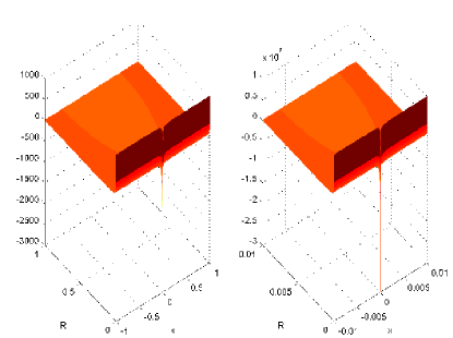
Figure 1: Three-particle potential at $y=0$

The point $R=x=y=0$ is a collision point of the three particles. However, because of the unstable nature of this point and the narrowness of the negative potential region, this configuration will not be observed in a classical equilibrium setting. Of course, in a full ergodic chaotic system, confined to a finite volume, there would be some small occurrence probability. This situation was studied before [14], but the nevertheless non-vanishing quasi-collision rates that are obtained are too small to be of practical interest. In addition, to try and induce collisions in a confined system by chaotizing it, for example, by a temperature increase or a sonic wave not only risks the destruction of the confinement cage but also, because of the chaotic nature of the event, leads to basically irreproducible events.

Therefore, for quasi-collisions of many-body systems, involving both attractive and repulsive forces, to be of practical interest, in chemical or nuclear situations, it seems better to explore the quantum nature of the problem, in particular the scar nature of classically unstable quantum states. And then to address directly these states by quantum control techniques. A precondition is, of course, to establish the existence of such states. A first step in this direction was taken in [15] where a configuration of two positive charges in a octahedral cage was considered, the vertices of the cage being occupied by atoms with a partially filled shell. One-electron energy levels were studied in a basis that contained both $d$-orbitals centered at the vertices and $s$-orbitals centered at the positive charges. Although the ground states that are obtained correspond to large separations of the positive charges, some excited states were found that have large quasi-collision probabilities. In this paper a similar situation is studied, with two positive and one negative charge confined in a cage, but using a much larger state basis. For the diagonalization of the Hamiltonian, a finite-difference method is used, the size of the basis being the number of discretization points in the cage. Up to $2.19\times 10^{4}$ basis states were used. Denoting by $R$ the distance between the positively charged particles and by $z$ all other coordinates and labelling the eigenstates as $\psi\left(R,z\right)$, the quasi-collision probability is defined as

$$I_{0}=\int dz\left|\psi\left(0,z\right)\right|^{2}$$ (2)

As in [15], many excited states with $I_{0}\neq 0$ are found.

It must be pointed out that such states which have a scar-like nature can only be observed in a fully dynamical treatment when $R$ is a dynamical variable and not an average value obtained by some a-posteriori minimization problem. In the next section this point is emphasized by exhibiting the limitations of the quasi-static approximation for the three-body problem.

2 A charged three-body problem: limitations of the quasi-static approximation

Here one deals with a Coulomb system of two positively $Z-$charged particles of mass $M$ interacting with a particle of mass $m$ and unit negative charge. And, for the moment, one deals with the problem in the full $3-$space, not on a confined volume. Define prolate spheroidal coordinates (Fig.2),

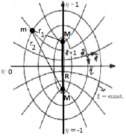
Figure 2: Prolate spheroidal coordinates

with $1\leq\xi<\infty$ and $-1\leq\eta\leq 1$ being the spheroidal coordinates in the plane of the three particles and $\phi$ the angular coordinate of the mass $m$ particle around the $z-$axis defined by the two mass $M$ particles. In the reference frame of the $z-$axis with the $M$ particles placed symmetrically about the origin, $R/2$ is the only dynamical variable of the mass $M$ particles. In this frame the Coulomb interaction Hamiltonian is

$$H=-\frac{\hslash^{2}}{2M}8\frac{\partial^{2}}{\partial R^{2}}-\frac{\hslash^{2}}{2m}\Delta_{m,1}+V\left(R,\xi,\eta\right)$$ (3)

with

$$\Delta_{m,1}=\frac{4}{R^{2}\left(\xi^{2}-\eta^{2}\right)}\left\{\frac{\partial}{\partial\xi}\left(\xi^{2}-1\right)\frac{\partial}{\partial\xi}+\frac{\partial}{\partial\eta}\left(1-\eta^{2}\right)\frac{\partial}{\partial\eta}+\frac{\partial}{\partial\phi}\left(\frac{\xi^{2}-\eta^{2}}{\left(\xi^{2}-1\right)\left(1-\eta^{2}\right)}\right)\frac{\partial}{\partial\phi}\right\}$$ (4)

and

$$V\left(R,\xi,\eta\right)=\frac{Ze^{2}}{4\pi\varepsilon_{0}}\left(\frac{Z}{R}-\frac{2}{R\left(\xi-\eta\right)}-\frac{2}{R\left(\xi+\eta\right)}\right)$$ (5)

$Z$ being the ratio of the charges of the mass $M$ and the mass $m$ particles. With $G^{2}=\frac{mZe^{2}}{2\hslash^{2}\pi\varepsilon_{0}}$ and $\mu=\frac{m}{M}$ one has

$$\frac{2m}{\hslash^{2}}H=-8\mu\frac{\partial^{2}}{\partial R^{2}}-\Delta_{m,1}+\frac{G^{2}}{R}\left(Z-\frac{4\xi}{\xi^{2}-\eta^{2}}\right)$$ (6)

In the usual treatments of the ground and excited states of the ionized hydrogen molecule, $R$ is treated as a parameter to be fixed by minimizing the energy associated to each $\psi\left(\xi,\eta\right)$ wave function. This provides for each state (ground or excited) the mean value of the coordinate $R$. If, however, one wants information on the quasi-collision probability of the particles, the important issue is the value the wave function at $R=0$, hence $R$ should have been treated as a dynamical variable. Because $R$ enters in the second and third term of Eq.(6) with different powers, a complete separation of variables is not possible. A partial separation which, although better than a purely static assumption for the mass $M$ particles, is not accurate is to solve the following eigenvalue problem for each fixed $R$

$$\left\{-\frac{R}{4}\Delta_{m,1}+\frac{G^{2}}{4}\left(Z-\frac{4\xi}{\xi^{2}-\eta^{2}}\right)\right\}\psi_{\beta,\alpha}\left(R,\xi,\eta\right)\chi_{\alpha}\left(\phi\right)=\lambda_{\beta,\alpha}\left(R\right)\psi_{\beta,\alpha}\left(R,\xi,\eta\right)\chi_{\alpha}\left(\phi\right)$$ (7)

and then, when for each set of quantum numbers $\beta,\alpha$ (associated to the variables $\xi,\eta$ and $\phi$) the function $\lambda_{\beta,\alpha}\left(R\right)$ is found, to obtain the $R-$dependence of the wave function from

$$\left\{-8\mu\frac{\partial^{2}}{\partial R^{2}}+\frac{4\lambda_{\beta,\alpha}\left(R\right)}{R}\right\}\psi_{\beta,\alpha}\left(R,\xi,\eta\right)\chi_{\alpha}\left(\phi\right)=\frac{2m}{\hslash^{2}}E\psi_{\beta,\alpha}\left(R,\xi,\eta\right)\chi_{\alpha}\left(\phi\right)$$

$V_{\beta,\alpha}\left(R\right)=\frac{4\lambda_{\beta,\alpha}\left(R\right)}{R}$ being an effective potential for the $R-$dependence of the wave function. Let $\chi_{\alpha}\left(\phi\right)=\exp\left(i\alpha\phi\right)$ with $\alpha$ an integer. Now, for each fixed $R$, separation of the variables $\psi_{\beta,\alpha}\left(R,\xi,\eta\right)=\psi_{\beta,\alpha}\left(R,\xi\right)\psi_{\beta,\alpha}\left(R,\eta\right)$ yields

$$\left\{\frac{\partial}{\partial\xi}\left(\xi^{2}-1\right)\frac{\partial}{\partial\xi}-\frac{\alpha^{2}}{\xi^{2}-1}-R\frac{G^{2}}{4}\left(Z\xi^{2}-4\xi\right)-\Lambda_{\alpha,R}\right\}\psi_{\beta,\alpha}\left(R,\xi\right)=-R\lambda_{\beta,\alpha}\left(R\right)\xi^{2}\psi_{\beta,\alpha}\left(R,\xi\right)$$

$$\left\{\frac{\partial}{\partial\eta}\left(1-\eta^{2}\right)\frac{\partial}{\partial\eta}-\frac{\alpha^{2}}{1-\eta^{2}}+R\frac{G^{2}}{4}Z\eta^{2}+\Lambda_{\alpha,R}\right\}\psi_{\beta,\alpha}\left(R,\eta\right)=R\lambda_{\beta,\alpha}\left(R\right)\eta^{2}\psi_{\beta,\alpha}\left(R,\eta\right)$$ (8)

$\Lambda_{\alpha,R}$ being the separation constant. Solving the joint eigenvalue problem (8) each $R-$family of eigenstates yields the $\lambda_{\beta,\alpha}\left(R\right)$ functions. However if one is only interested in the nature of the effective $R-$potential, the problem may be further simplified by fixing the coordinates to a fixed value. For example, with $\xi=1$ and $\eta=0$ in the case $\alpha=0$, one obtains from (8)

$$V_{\beta,0}\left(R\right)=-G^{2}\left(\frac{4-Z}{R}\right)+\frac{4}{R^{2}}\psi_{\beta,0}^{-1}\left(R,1,0\right)\left.\left(-\frac{\partial^{2}\psi_{\beta,0}}{\partial\eta^{2}}-2\frac{\partial\psi_{\beta,0}}{\partial\xi}\right)\right|_{\xi=1,\eta=0}$$ (9)

Therefore the effective $R-$potential contains a $1/R$ term which is attractive for $Z<4$ and a repulsive term originating from the kinetic part of the Hamiltonian. Because of the $1/R^{2}$ factor, this last term is expected to be strongly repulsive at $R=0$ for the eigenstates of Eq.(7), precluding any quasi-collisions. In fact this result is to be expected and is a result of the factorized way the calculation is performed. Separating the $R-$dynamics (of the mass $M$ particles) from the dynamics of the mass $m$ particle, what one is studying is the $R-$dynamics in the mean field of the other particle, not the simultaneous quantum fluctuations of all particles to the unstable or the tiny energetically favorable regions of configuration space as described in Section $1$. Therefore to study this phenomena, one should consider the joint dynamics of all particles. This will be the subject of the next Section.

In the present Section prolate spheroidal coordinates were used because they are appropriate for the factorized problem and have traditionally been used for that purpose. However to deal with the full dynamical problem they are not very convenient and, in addition, also not appropriate for a system confined in a finite volume because physical space coordinates are defined as multiples of $R$, namely

$$x=\frac{R}{2}\xi\eta;\;y=\frac{R\sin\phi}{2}\sqrt{\left(\xi^{2}-1\right)\left(1-\eta^{2}\right)};\;z=\frac{R\cos\phi}{2}\sqrt{\left(\xi^{2}-1\right)\left(1-\eta^{2}\right)}.$$

Therefore for a small $R$ the $\xi-$coordinate must be extremely large for a physically finite volume.

3 The dynamical problem

Here one addresses the joint dynamical problem of the $3$ particles. The reference frame is chosen with the $y-$axis along the line joining the two mass $M$ particles and the origin at the middle point, their $y-$coordinates being $R/2$ and $-R/2$. The three-dimensional coordinates are $\left(x,y,\theta\right)$, $\theta$ being the angle of rotation of the plane of the three particles. These are coordinates for a finite volume cylinder, with the choice $x\in[-L,L]$, $y\in[-L,L]$, $\theta\in[0,\pi]$ (Fig.3). The ”radial” variable $x$ is chosen in a symmetrical way because this is more convenient to fix the boundary conditions.

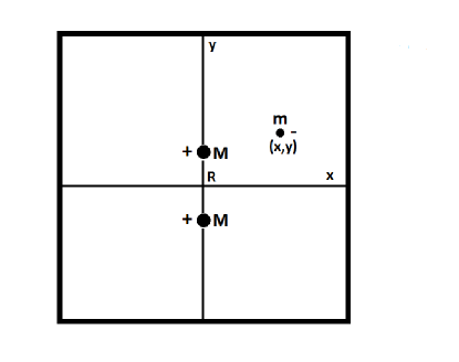
Figure 3: Three particles in a cylindrical box. A section of the box at fixed $\theta$

The Hamiltonian is

$$\frac{2m}{\hslash^{2}}H=-8\mu\frac{\partial^{2}}{\partial R^{2}}-\Delta_{m,2}+\frac{2m}{\hslash^{2}}V\left(R,x,y\right)$$ (10)

with

$$\Delta_{m,2}=\frac{1}{x}\frac{\partial}{\partial x}\left(x\frac{\partial}{\partial x}\right)+\frac{\partial^{2}}{\partial y^{2}}+\frac{1}{x^{2}}\frac{\partial^{2}}{\partial\theta^{2}}$$ (11)

$$V\left(R,x,y\right)=\frac{Ze^{2}}{4\pi\varepsilon_{0}}\left\{\frac{Z}{R}-\frac{1}{\sqrt{x^{2}+\left(\frac{R}{2}-y\right)^{2}}}-\frac{1}{\sqrt{x^{2}+\left(\frac{R}{2}+y\right)^{2}}}\right\}$$ (12)

The $\theta$ dependence is taken care of by factorization with $\chi_{\alpha}\left(\theta\right)=\exp\left(i\alpha\theta\right)$ and two cases will be studied: first, the case of two variables $\left(R,x\right)$, that is, the mass $m$ particle constrained to move along the $x-$axis and then the three variables $\left(R,x,y\right)$ case. In both cases one considers the angular symmetric situation $\left(\alpha=0\right)$.

To fully grasp the nature of the dynamical problem, in the two-variables case, both the 2-dimensional (motion in the plane) and the 3-dimensional (motion along the $x-$axis in 3 dimensions) cases are considered. For the three-variables case only 3-dimensional motion will be considered.

The interest of the dimensionally restricted studies is not purely academic because, for systems confined in a molecular cage, the orbitals of the containing molecules, that form the cage, may impose further dimensional constraints on the confined particles.

In a confined volume the natural boundary condition to impose is the vanishing of the wave function at the boundaries. A particularly efficient way to obtain a very large number of eigenvalues and eigenfunctions of the operator is a finite difference method on a grid using a fast diagonalization routine (see for example [16]). The number of eigenfunctions that is obtained may always be improved by using finer and finer grids. Different degrees of approximation may be used to construct the matrix representation of the operators. In practice there is a trade-off between using higher-order operator representations and finer grids with lower order representations, which lead to sparser matrices. In the following, the results obtained with a finite difference diagonalization method are presented. Here 5-points approximations have been used for the derivatives.

To work with dimensionless quantities one actually computes the spectrum of $\frac{2m}{\hslash^{2}G^{4}}H_{2}$, the corresponding length variables being $G^{2}R$, $G^{2}x$ and $G^{2}y$. Recall that $G^{2}=\frac{mZe^{2}}{2\hslash^{2}\pi\varepsilon_{0}}$.

3.1 Two variables (R,x), $\alpha=0$

3.1.1 Motion along the $x-$axis in the plane

$$\frac{2m}{\hslash^{2}G^{4}}H_{2}^{(P)}=-8\mu\frac{\partial^{2}}{\partial\left(G^{2}R\right)^{2}}-\frac{\partial^{2}}{\partial\left(G^{2}x\right)^{2}}+\left\{\frac{Z}{G^{2}R}-\frac{2}{\sqrt{\left(G^{2}x\right)^{2}+\left(\frac{G^{2}R}{2}\right)^{2}}}\right\}$$ (13)

For a $150\times 150$ two-dimensional grid in the $\left(\tilde{x}=G^{2}x,\tilde{R}=G^{2}R\right)-$plane in a square box with $\tilde{x}$ and $\tilde{R}$ $\in[-15,15]$ the results are summarized in the Figs.4 and 5.

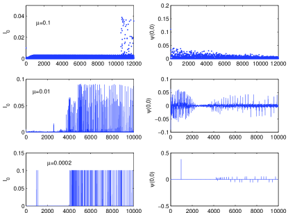
Figure 4: $I_{0}$ and $\psi\left(0,0\right)$ at several $\mu$ ratios for motion along the $x-$axis in the plane

For several values of $\mu=\frac{m}{M}$ the left panels in Fig.4 show the value of

$$I_{0}=\int\left|\psi\left(\tilde{x},0\right)\right|^{2}d\tilde{x}$$

and the right panels $\psi\left(0,0\right)$, the eigenvector value at the origin. The number of eigenvalues listed in the figure is less than $1/2$ of the total number of eigenvalues, higher eigenvalues being less accurate in the finite difference method. $I_{0}$ is a measure of the quasi-collision probability of the two heavy positively charged particles. The first such state appears isolated high up in the spectrum, many other such states appearing even higher in the spectrum. Notice that although all these states have high values of $I_{0}$ they have different values at the origin $\psi\left(0,0\right)$. This means that although they all imply a high quasi-collision probability $\left(R=0\right)$, they have different spreading along the $x-$axis. The location of the first quasi-collision state (as well as the states for which there is a non-zero value of the wave function at the origin) move to lower energies as the $\mu$ ratio increases and, at $\mu=0.1$ even the ground state has $I_{0}\neq 0$. This means that mass (or effective mass) of the light particle is an important consideration. Fig.5 shows on the left panels the wave function of the ground state for $\mu=0.1$ and in the right panels the first quasi-collision state for $\mu=0.00027$.

Because all quantities in this paper are expressed in dimensionless quantities all the dynamical studies in this paper may be easily adapted to confined collisions in chemical or nuclear reactions. Actual lengths $L$ are related to dimensionless lengths $\overset{\char 126\relax}{L}$ by $L=G^{-2}\overset{\char 126\relax}{L}$ and actual energies $E$ are related to the eigenvalues $\overset{\char 126\relax}{E}$ of the dimensionless Hamiltonian $\frac{2m}{\hslash^{2}G^{4}}H$ by $E=\frac{\hslash^{2}G^{4}}{2m}\overset{\char 126\relax}{E}$. For definiteness, I will concentrate on the possibility of observing nuclear reactions when nuclei are confined in solid matter. Therefore quantitative estimates will be made for $m=$ the electron mass, $M=$ the deuteron mass. For these values $G^{2}=$ $\frac{mZe^{2}}{2\hslash^{2}\pi\varepsilon_{0}}=0.3779\times 10^{11}m^{-1};G^{-2}=0.2646\overset{\circ}{A}$ and $\tilde{x},\tilde{R}\in[-15,15]$ roughly corresponds to

confinement in a $8\times 8$ $\overset{\circ}{A}$ box. $\frac{m_{e}}{M_{D}}=0.00027$. The energy conversion factor is $\left(\frac{2m_{e}}{\hbar^{2}G^{4}}\right)^{-1}=54.4$ eV. Then, the binding energy of the ground state would be $120$ eV and the first quasi-collision state would be $160$ eV above the ground state. The proliferation of the other quasi-collision states occurs above $500$ eV. Although these results are obtained in a simplified situation of motion along the axis on the plane, they already indicate that spontaneous fusion of nuclei confined in solid matter either does not occur at all or, if occurring in some random exceptional event, is not a practical reproducible phenomenon. Consistent production of quasi-collision states requires excitation of the system to the low $x-$ray energy range.

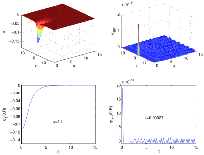
Figure 5: The ground state wave function at $\mu=0.1$ and the first quasi-collision state at $\mu=0.00027$

The results obtained in this subsection use a basis of $21904$ states. How the energy estimates for the quasi-collision states might depend on the number of basis states is discussed in 3.4.

3.1.2
Motion along the $x-$axis in the cylinder

$$\frac{2m}{\hslash^{2}G^{4}}H_{2}^{(C)}=-8\mu\frac{\partial^{2}}{\partial\left(G^{2}R\right)^{2}}-\frac{1}{G^{2}x}\frac{\partial}{\partial\left(G^{2}x\right)}\left(G^{2}x\frac{\partial}{\partial\left(G^{2}x\right)}\right)+\left\{\frac{Z}{G^{2}R}-\frac{2}{\sqrt{\left(G^{2}x\right)^{2}+\left(\frac{G^{2}R}{2}\right)^{2}}}\right\}$$ (14)

The situation here, as illustrated in Fig.6, is qualitatively similar to the plane motion case, the main difference being that a smaller binding energy of the ground state is obtained and the quasi-collision states occur higher in the spectrum. With the same choices as before for the physical parameters, the first one would be $389$ eV above the ground state with many others above $540$ eV.

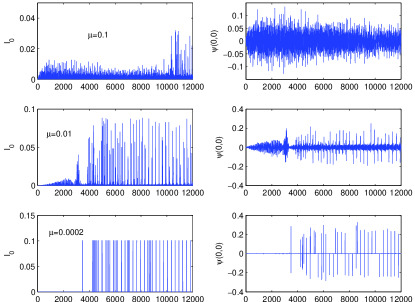
Figure 6: $I_{0}$ and $\psi\left(0,0\right)$ at several $\mu$ ratios for motion along the $x$-axis in the cylinder

3.2 Three variables (R,x,y), $\alpha=0$

Here only the motion in the cylinder case will be analyzed ($\tilde{R}=G^{2}R$; $\tilde{x}=G^{2}x$; $\widetilde{y}=G^{2}y$)

$$\frac{2m}{\hslash^{2}G^{4}}H_{3}=-8\mu\frac{\partial^{2}}{\partial\tilde{R}^{2}}-\frac{1}{\tilde{x}}\frac{\partial}{\partial\tilde{x}}\left(\tilde{x}\frac{\partial}{\partial\tilde{x}}\right)-\frac{\partial^{2}}{\partial\widetilde{y}^{2}}+\left\{\frac{Z}{\tilde{R}}-\frac{1}{\sqrt{\tilde{x}^{2}+\left(\frac{\tilde{R}}{2}-\widetilde{y}\right)^{2}}}-\frac{1}{\sqrt{\tilde{x}^{2}+\left(\frac{\tilde{R}}{2}+\widetilde{y}\right)^{2}}}\right\}$$ (15)

In the previous cases, when the motion is constrained to the $y=0$ axis, the reason why states with $I_{0}$ and $\psi\left(0,0\right)\neq 0$ only occur for relatively high excited states lies on the extreme narrowness of the negative potential region when $R=0$. Then the kinetic energy of the light particle implies an high energy contribution for localized states. In the three variables case one would expect the existence of such localized states to be even more energy demanding because of the instability of the potential singularity along the $y$ direction. Nevertheless it turns out that the spectrum situation is not very different from what it was before. Fig.7 (obtained with $21952$ basis states) shows the values of $I_{0}$,

$$I_{0}=\int\left|\psi\left(\tilde{x},\widetilde{y},0\right)\right|^{2}d\tilde{x}d\widetilde{y}$$

$\psi\left(0,0,0\right)$ and the corresponding dimensionless eigenvalue values $\lambda=\overset{\char 126\relax}{E}$, for $\mu=0.00027$.

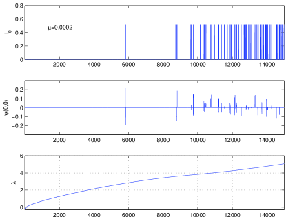
Figure 7: $I_{0}$, $\psi\left(0,0\right)$ and (dimensionless) eigenvalues for the three-variables case with $\mu=0.00027$

The first quasi-collision state occurs at $\widetilde{E}=2.8$ which would correspond to $152$ eV with many others after $3.59$ ($195$ eV). Excitation of these states are as before in the low $x-$ray energy range. Notice however that these values should only be considered as lower bounds for the excitation energies, because a smaller spatial density of basis states has been used, as compared to the one in the two previous subsections (see the discussion in 3.4).

3.3 Confinement and basis size effects

An important issue is the dependence of the quasi-collision states on the size of the confinement box and on the number of basis states that is used to compute the spectrum.

Concerning the dependence on the size of the confinement box it is found that the energies of the quasi-collision states grow when the size of the box decreases, but they appear earlier in the spectrum.

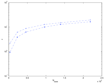
Figure 8: Dependence on the number of basis states of the energy of the first quasi-collision state (lower line) and the energy above which many other such states exist (upper line)

Of more interest for the correct estimation of the energy needed to excite the quasi-collision states is their dependence on the number of states used for the computation of the spectrum. Fig.8 shows the dependence on the number of basis states of the energy of the first quasi-collision state (lower line) and the energy above which many other such states exist (upper line). This calculation refers to the two-variables in the cylinder case of subsection 3.2. Whereas the ground state energy is found to be quite stable for sizes above 800, the quasi-collision energies still grow even at sizes above 20000. Therefore the values obtained in the previous subsections should be considered as lower bounds for the correct excitation energies, which however, from the behavior seen in the figure, should still be expected to be in the $x-$ray range for the physical parameters used here.

4 Quantum control of quasi-collisions

From the dynamical study of the previous section one sees that, in spite of the strong Coulomb barrier there indeed are ”quantum quasi-collision states” (in the sense of the definition before, $I_{0}\neq 0$) of the three particles. They are located at energies well above the ground state, the question being whether the system may be driven to these states by practical means. This is a typical question of quantum control. At the present day the only viable way to quantum control is through the electric field of laser pulses with, eventually, as will be seen later, a tuning effect of magnetic fields.

In the dipole approximation the Hamiltonian for particles interacting with the electromagnetic wave of a laser pulse is

$$i\hslash\frac{\partial}{\partial t}\psi\left(x_{j},t\right)=\sum_{j}\left\{H_{0}-e_{j}x_{j}\cdot E\left(t\right)\right\}\psi\left(x_{j},t\right)$$ (16)

with

$$H_{0}=\sum_{j}-\frac{\hslash^{2}}{2m_{j}}\nabla_{j}^{2}+V\left(x_{j}\right)$$ (17)

$V\left(x_{j}\right)$ being the Coulomb interactions in (13 - 15) or these interactions complemented by an external magnetic field, as described later. Let the eigenstates of $H_{0}$ be known

$$H_{0}\phi_{k}=\varepsilon_{k}\phi_{k}$$ (18)

The goal is, starting from an initial state $\phi_{i}$ (typically the ground state), to lead the system to a desired final state $\phi_{f}$ (here a quasi-collision state). Treating the term $H_{I}=-\sum_{j}e_{j}x_{j}\cdot E\left(t\right)=-\sum_{j}e_{j}E\exp\left(i\omega t\right)$ as a perturbation, the evolution operator $U_{I}\left(T,0\right)$ in the interaction picture is

$$U_{I}\left(T,0\right)=1-\frac{i}{\hslash}\int_{0}^{T}H_{I}\left(t^{\prime}\right)U_{I}\left(t^{\prime},0\right)dt^{\prime}$$ (19)

with

$$H_{I}\left(t\right)=-\sum_{j}e_{j}Ee^{i\omega t}e^{\frac{i}{\hslash}H_{0}t}x_{j}e^{-\frac{i}{\hslash}H_{0}t}$$ (20)

$$e^{\frac{i}{\hslash}H_{0}t}x_{j}e^{-\frac{i}{\hslash}H_{0}t}=x_{j}-it\frac{\hslash}{m_{j}}x_{j}\frac{\partial}{\partial x_{j}}+t^{2}\frac{\hslash}{4m^{2}}V^{\prime}\left(x_{j}\right)+\cdots$$ (21)

The transition probability from the initial state $\phi_{i}$ to the final state $\phi_{f}$ is obtained from $\left|\left\langle\phi_{f}\left|U\left(T,0\right)\right|\phi_{i}\right\rangle\right|^{2}$. When the desired final state is a quasi-collision one, the contribution of the $U\left(T,0\right)$ series will be strongly suppressed by the $x_{j}$ terms, which vanish at the collision. Therefore one expects the leading contribution to be

$$\left|\frac{\hslash E}{4m^{2}}\int_{0}^{T}e^{-\frac{i}{\hslash}t\Delta\varepsilon}e^{it\omega}t^{2}\left\langle\phi_{f}\left|V^{{}^{\prime}}\left(x_{j}\right)\right|\phi_{i}\right\rangle\right|$$ (22)

$\Delta\varepsilon$ being the energy difference between $\phi_{f}$ and $\phi_{i}$. From (22) one concludes that in addition to a laser frequency tuned to $\Delta\varepsilon$, long duration pulses should be favored.

4.1 Spectrum modulation by a constant magnetic field

Here, one analyses the shifts in the spectra studied in Section 3 which might be obtained with an external static (or slowly varying) magnetic field. With an external field the electromagnetic contribution to the Hamiltonian is

$$H_{em}=\frac{1}{2m}\left(p-eA\left(x,t\right)\right)^{2}+e\Phi\left(x,t\right)$$ (23)

which in the Coulomb gauge, $\nabla\cdot A=\Phi=0$, becomes

$$H_{em}=-\frac{\hslash^{2}}{2m}\nabla^{2}+i\frac{e\hslash}{m}A\cdot\nabla+\frac{e^{2}}{2m}A^{2}$$ (24)

The two interaction terms are of a different nature, the first one being called the paramagnetic  term and the last the diamagnetic term. For a stationary uniform magnetic field, let

$$A\left(x\right)=-\frac{1}{2}x\times B=-\frac{1}{2}\left\{e_{x}\left(yB_{z}-zB_{y}\right)+e_{y}\left(zB_{x}-xB_{z}\right)+e_{z}\left(xB_{y}-yB_{x}\right)\right\}$$ (25)

Then the paramagnetic term is

$$i\frac{e\hslash}{m}A\cdot\nabla=-\frac{e}{2m}L\cdot B$$ (26)

with

$$L=x\times\left(-i\hslash\nabla\right)$$ (27)

For the simplest cases studied in Section 3, $L=0$, the paramagnetic term term vanishes, the only contribution coming from the diamagnetic term. The contribution of the diamagnetic term to the dimensionless Hamiltonians $\frac{2m}{\hslash^{2}G^{4}}H$ is

$$\frac{e^{2}}{\hslash^{2}G^{8}}\left(\frac{1}{4}\widetilde{x}^{2}\left(B_{z}^{2}+B_{y}^{2}\right)+\frac{Z^{2}\mu}{4}\widetilde{R}^{2}\left(B_{z}^{2}+B_{x}^{2}\right)\right)$$ (28)

This adds to the dynamics an harmonic contribution which would favor a closer proximity of the particles. Notice however that $\frac{e}{\hslash G^{4}}$ is the factor which multiplies the physical fields which, for the physical parameters used before (three-body quasi-collision of deuterons), is extremely small, of order $1.06\times 10^{-6}$. Therefore the contribution of the diamagnetic interaction term would be too small to be of practical relevance in this case. It might however be relevant for other physical parameters, namely chemical reactions of confined atoms.

By contrast the corresponding factor in the paramagnetic interaction term would be $\frac{e}{\hslash^{2}G^{4}}$ and physically reasonable magnetic fields may induce appreciable spectrum shifts in the $L\neq 0$ case.

5 Remarks and conclusions

1 - Properties of confined systems may greatly differ from similar systems in free spaces. Exploration of new pathways for chemical or nuclear reactions might be a promising application for atoms or nuclei confined in molecular cages.

2 - In what concerns the possibility to observe fusion reactions by many-body effects when nuclei are confined in a cage, the main conclusion of this paper is that spontaneous occurrence of these events is quite improbable and if they occur at all under ergodic situations they will be basically uncontrollable and irreproducible. Nevertheless, considering the molecular cage merely as a confinement device, reproducible quasi-collisions might be induced by quantum control techniques. This two-step protocol would be what elsewhere [15] has been called ”hybrid fusion”.

3 - Quantum control is a technique that has had in recent years remarkable development. Learning and adaptive techniques [17] [18], optimal control [19], unitary and non-unitary [20] [21] evolution methods have been developed, even infinite-dimensional spaces once considered to be uncontrollable have been proved to yield to full quantum control [22] [23]. Here only a very basic discussion of the control requirements has been performed. Once the detailed nature of the molecular cage is specified, all the developed techniques may be applied to smoothly drive the system to the quasi-collision states.

4 - For the fusion situation that was specified, excitation of the quasi-collision states seemed to require laser pulses on the $x-$ray range. It is interesting to note that also on a recent experiment some authors [24] suggest the induction of fusion reactions in a crystal by $x-$rays.

5 - A point that should be recalled when identifying fusion reactions induced by many-body effects is that the reaction channels and final products might be different from those of the two-body reaction [25] [14].

6 - Here the problem of three-particles in a single molecular cage was considered and quantum control of elementary quasi-collision states has been emphasized. Another situation where similar quasi-collisions might occur is when many such contiguous cages communicate and the collective system is sufficiently excited to be describable by a chaotic ergodic measure. This is the situation studied in [14], where small but non-negligible quasi-collisions rates were found. However, the chaotic nature of the collective events would render them either difficult to control or irreproducible and therefore of little interest for steady energy production applications. This situation might however be relevant as a correction to the dynamics of stellar models.

References

- [1] P. Ballester, M. Fujita and J. Rebek (Ed.) , Molecular Containers, a special issue of Chem. Soc. Rev. 44 (2015).
- [2] Masumeh Foroutana, S. M. Fatemi, and F. Esmaeilian; A review of the structure and dynamics of nanoconfined water and ionic liquids via molecular dynamics simulation, Eur. Phys. J. E (2017) 40:19.
- [3] T Sako and G. H. F. Diercksen; Confined quantum systems: a comparison of the spectral properties of the two-electron quantum dot, the negative hydrogen ion and the helium atom, Journal of Physics B: Atomic, Molecular and Optical Physics 36 (2003) 1681-1702.
- [4] A. I. Shnirelman; On the asymptotic properties of eigenfunctions in the regions of chaotic motion, Usp. Mat. Nauk. 29 (1974) 181-182.
- [5] S. Zelditch; Uniform distribution of eigenfunctions on compact hyperbolic surfaces, Duke Math. J. 55 (1987) 919-941.
- [6] Y. Colin de Verdière: Ergodicité et fonctions propres du laplacien, Commun. Mth. Phys. 102 (1985) 497-502.
- [7] P. B. Wilkinson, T. M. Fromhold, L. Eaves, F. W. Sheard, N. Miura and T. Takamasu, Observation of scarred wavefunctions in a quantum well with chaotic electron dynamics, Nature 380 (1996) 608-610.
- [8] E. J. Heller; Bound-state eigenfunctions of classically chaotic Hamiltonian systems: Scars of periodic orbits, Phys. Rev. Lett. 53 (1984) 1515-1518.
- [9] E. B. Bogomolny; Smoothed wave functions of chaotic quantum systems, Physica D 31 (1988) 169-189.
- [10] M. V. Berry; Quantum scars of classical closed orbits in phase space, Proc. R. Soc. London A 423 (1989) 219-231.
- [11] M. Feingold, R. G. Littlejohn, S. B. Solina, J. S. Pehling and O. Piro; Scars in billiards: The phase space approach, Phys. Lett. A 146 (1990) 199-203.
- [12] R. Vilela Mendes; Saddle scars: existence and applications, Phys. Lett. A 239 (1998) 223-227.
- [13] R. Vilela Mendes; Collision states and scar effects in charged three-body problems, Phys. Lett. A 233 (1997) 265-273.
- [14] R. Vilela Mendes; Ergodic motion and near-collisions in a Coulomb system, Modern Physics Lett. B 5 (1991) 1179-1190.
- [15] R. Vilela Mendes; Quantum collision states for positive charges in an octahedral cage, Int. J. Hydrogen Energy 28 (2003) 125-129.
- [16] D. X. Ogburn et al.; A finite difference construction of the spheroidal wave functions, Computer Phys. Commun. 185 (2014) 244-253.
- [17] M. Shapiro and P. Brumer; Quantum Control of Molecular Processes, 2nd Edition, Wiley 2012.
- [18] C. Brif, R. Chakrabarti1 and H. Rabitz; Control of quantum phenomena: past, present and future, New Journal of Physics 12 (2010) 075008.
- [19] S. van Frank et. al; Optimal control of complex atomic quantum systems, Scientific Reports 6 (2016) 34187.
- [20] R. Vilela Mendes and V. I. Man’ko; Quantum control and the Strocchi map, Phys. Rev. A 67 (2003) 053404.
- [21] A. Mandilara and J. W. Clark; Probabilistic quantum control via indirect measurement, Phys. Rev. A 71 (2005) 013406.
- [22] W. Karwowski and R. Vilela Mendes; Quantum control in infinite dimensions, Phys. Lett. A 322 (2004) 282–285.
- [23] R. Vilela Mendes and V. I. Man’ko; On the problem of quantum control in infinite dimensions, J. Phys. A: Math. Theor. 44 (2011) 135302.
- [24] V. B. Belyaev, M. B. Miller, J. Otto and S. A. Rakityansky; Nuclear fusion induced by x rays in a crystal, Phys. Rev. C 93 (2016) 034622.
- [25] R. Vilela Mendes; Three body effects and neutron suppression in cold fusion, IFM preprint 10/89, http://inspirehep.net/record/280227.