Dynamical Instability of Charged Gaseous Cylinder

Abstract

In this paper, we discuss dynamical instability of charged dissipative cylinder under radial oscillations. For this purpose, we follow the Eulerian and Lagrangian approaches to evaluate linearized perturbed equation of motion. We formulate perturbed pressure in terms of adiabatic index by applying the conservation of baryon numbers. A variational principle is established to determine characteristic frequencies of oscillation which define stability criteria for gaseous cylinder. We compute the ranges of radii as well as adiabatic index for both charged and uncharged cases in Newtonian and post-Newtonian limits. We conclude that dynamical instability occurs in the presence of charge if the gaseous cylinder contracts to the radius $R_{*}$.

1 Introduction

A comprehensive study of collapsing systems and structure formation of self-gravitating objects reveal interesting physical perspectives. Charged self-gravitating objects may undergo various evolutionary phases during gravitational collapse that results into charged black holes or naked singularities. The stability of these solutions under fluctuations has remarkable significance in general relativity (GR). Initially, any stable system remains in state of hydrostatic equilibrium unless its own gravity overcomes the pressure which causes the matter to collapse. The collapsing system contracts to a point under the influence of its own gravity leading to compact objects.

The dynamical instability of massive stars can be studied in Newtonian as well as post-Newtonian (pN) regimes (Ayal et al., 2001; Marek et al., 2006). This provides a platform to evaluate ranges of deviation and level of consistency between GR and Newton gravity. The analysis becomes ambiguous in strong-field regimes due to non-linear terms, hence the weak-field approximation schemes are used as an effective tool. Chandrasekhar (1964) was the pioneer who discussed the concept of dynamical instability of gaseous sphere by taking Newtonian perfect fluid in terms of adiabatic index. He followed Eulerian approach for linearized perturbed hydrodynamic equations and established a variational principle to find characteristic frequencies in Newtonian and pN limits. He also studied dynamical stability of sphere under radial and non-radial oscillations at pN limit (Chandrasekhar, 1965).

Herrera et al. (1989) investigated dynamical instability of spherical system under perturbations by taking non-adiabatic fluid and found that the instability range increases in Newtonian limit but decreases in pN limit. Later, many researchers explored the influence of various physical parameters on the dynamical instability of self-gravitating systems under radial/non-radial perturbations (Chan et al., 1994; Nunez et al., 2007; Sharif & Azam, 2012). There has also been an extensive literature on the study of cylindrical gravitational collapse with and without electromagnetic field (Sharif & Ahmad, 2007; Di Prisco et al., 2009; Sharif & Abbas, 2011). Sharif & Azam (2013) studied dynamical instability of anisotropic collapsing cylinder in the context of expansion-free model.

It is well-known that various physical aspects of matter distribution play substantial role in the dynamical evolution of self-gravitating systems. A star requires more electromagnetic charge for its stability in a strong gravitational field. The dynamical instability of collapsing systems in the presence of electromagnetic field has a primordial history starting with Rosseland (Rosseland, 1924). Stettner (1973) discussed the role of surface charge in increasing stability of system with uniform density. Glazer (1976) studied dynamical stability of sphere under radial pulsations in the presence of electric charge. Ghezzi (2005) found that neutron stars having charge greater than the extreme value would explode. Sharif & Azam (2012); Sharif & Bhatti (2013); Sharif & Mumtaz (2016) studied the influence of electric charge on dynamical instability of collapsing systems at Newtonian and pN regimes.

In this paper, we study the impact of electromagnetic field on dynamical instability of cylindrically symmetric collapsing system by following Chandrasekhar approach (Chandrasekhar, 1964). The format of the paper is as follows. In section 2, we provide some basic equations and matter distribution for cylindrical geometry. Section 3 deals with equations of motion under radial oscillations following the Eulerian approach. We also formulate perturbed pressure and adiabatic index in terms of Lagrangian displacement by using conservation of baryon number. Section 4 is devoted to find conditions for dynamical instability of homogeneous cylinder. Finally, we conclude our results in the last section.

2 Field Equations and Matter Configuration

We consider a cylindrically symmetric system in the interior region given by

$$ds^{2}=-A^{2}(t,r)dt^{2}+B^{2}(t,r)dr^{2}+C^{2}(t,r)d\theta^{2}+dz^{2},$$ (1)

where the following restrictions on coordinates are taken to preserve symmetry

$$-\infty<t<\infty,\quad 0\leq r<\infty,\quad 0\leq\theta\leq 2\pi,\quad-\infty<z<\infty.$$

The corresponding Einstein field equations are given by

$$\frac{8\pi G}{c^{4}}T_{0}^{0} = \frac{1}{B^{2}}\left\{\frac{C^{\prime\prime}}{C}-\frac{B^{\prime}C^{\prime}}{BC}\right\}-\frac{\dot{B}\dot{C}}{A^{2}BC},$$ (2)

$$\frac{8\pi G}{c^{4}}T_{1}^{1} = \frac{1}{A^{2}}\left\{\frac{\dot{A}\dot{C}}{AC}-\frac{\ddot{C}}{C}\right\}+\frac{A^{\prime}C^{\prime}}{AB^{2}C},$$ (3)

$$\frac{8\pi G}{c^{4}}T_{2}^{2} = \frac{1}{AB}\left\{\frac{A^{\prime\prime}}{B}-\frac{\ddot{B}}{A}+{\frac{\dot{A}\dot{B}}{A^{2}}-\frac{A^{\prime}B^{\prime}}{B^{2}}}\right\},$$ (4)

$$\frac{8\pi G}{c^{4}}T_{3}^{3} = \frac{A^{\prime\prime}}{AB^{2}}-\frac{\ddot{B}}{A^{2}B}+\frac{\dot{A}\dot{B}}{A^{3}B}-\frac{A^{\prime}B^{\prime}}{AB^{3}}+\frac{\dot{A}\dot{C}}{A^{3}C}-\frac{\ddot{C}}{A^{2}C}$$ (5)

$$- \frac{B^{\prime}C^{\prime}}{B^{3}C}+\frac{C^{\prime\prime}}{B^{2}C}+\frac{A^{\prime}C^{\prime}}{AB^{2}C}-\frac{\dot{B}\dot{C}}{A^{2}BC},$$

$$\frac{8\pi G}{c^{4}}T_{0}^{1} = \frac{1}{B^{2}}\left\{\frac{A^{\prime}\dot{C}}{AC}+\frac{\dot{B}C^{\prime}}{BC}-\frac{\dot{C}^{\prime}}{C}\right\},$$ (6)

where dot and prime denote derivatives with respect to $t$ and $r$, respectively. The matter source is assumed to be locally charged dissipative perfect fluid defined by

$$T_{\nu}^{\mu}=(\sigma+p)u^{\mu}u_{\nu}+p\delta_{\nu}^{\mu}+q^{\mu}u_{\nu}+q_{\nu}u^{\mu}+\frac{1}{4\pi}[F_{\nu\rho}F^{\mu\rho}-\frac{1}{4}\delta_{\nu}^{\mu}F_{\rho\lambda}F^{\rho\lambda}],$$ (7)

where $p$ is the isotropic pressure, $\sigma$ is the energy density, $F_{\mu\rho}$ is the Maxwell field tensor, $u^{\mu}=\frac{dx^{\mu}}{ds}$ and $q^{\mu}$ represent four velocity and radial heat flux, respectively satisfying $q_{\mu}u^{\mu}=0$. Also, we have

$$u^{\mu}=A^{-1}\delta^{\mu}_{0},\quad q^{\mu}=q\delta^{\mu}_{1},\quad u^{\mu}u_{\mu}=-1.$$

We can define the electromagnetic field tensor in terms of four potential as $F_{\mu\nu}=\Phi_{\nu;\mu}-\Phi_{\mu;\nu}$, which satisfies the Maxwell field equations

$$F^{\mu\nu}_{~{};\nu}=4\pi J^{\mu},\quad F_{[\mu\nu,\rho]}=0,$$

where $J^{\mu}=\tilde{\rho}u^{\mu}$ is the four current. The conservation equation, $J^{\mu}_{;\mu}=0$, yields

$$Q(r)=4\pi\int_{0}^{r}\zeta BCdr,$$

which is the total amount of charge within cylinder. We define the electric field intensity as

$$E(t,r)=\frac{Q(r)}{2\pi C}.$$ (8)

The conservation of energy-momentum tensor leads to the following relations

$$\frac{\partial T_{0}^{0}}{\partial t}+\frac{\partial T_{1}^{0}}{\partial r}+\frac{\dot{B}}{B}\left(T_{0}^{0}-T_{1}^{1}\right)+T_{0}^{1}\left(\frac{B^{\prime}}{B}+\frac{A^{\prime}}{A}\right)=0,$$ (9)

$$\frac{\partial T_{1}^{0}}{\partial t}+\frac{\partial T_{1}^{1}}{\partial r}+\frac{A^{\prime}}{A}\left(T_{1}^{1}-T_{0}^{0}\right)+\left(\frac{\dot{A}}{A}+\frac{\dot{B}}{B}\right)T_{1}^{0}=0,$$ (10)

where $T_{0}^{1}=-\frac{A^{2}}{B^{2}}T_{1}^{0}$. The components of energy-momentum tensor are

$$T^{0}_{0}=-\sigma+\frac{\pi}{2}E^{2},\quad T^{1}_{1}=p+\frac{\pi}{2}E^{2},\quad T^{2}_{2}=T^{3}_{3}=p-\frac{\pi}{2}E^{2}.$$

In hydrostatic equilibrium, all the quantities governing motion remain time independent. In this context, Eqs.(2), (3) and (10) become

$$\frac{d}{dr}\left(\frac{C_{0}^{\prime}}{B_{0}}\right) = \frac{8\pi G}{c^{4}}B_{0}C_{0}\left(-\sigma_{0}+\frac{\pi E^{2}}{2}\right),$$ (11)

$$\frac{dA_{0}}{dr}\frac{dC_{0}}{dr} = \frac{8\pi G}{c^{4}}A_{0}B_{0}^{2}C_{0}\left(p_{0}+\frac{\pi E^{2}}{2}\right),$$ (12)

$$(\sigma_{0}+p_{0})\frac{dA_{0}}{dr} = -A_{0}\frac{d}{dr}\left(p_{0}+\frac{\pi E^{2}}{2}\right),$$ (13)

where zero suffix describes equilibrium state of the surface stresses. We also have a useful relation through Eqs.(2) and (3) given by

$$\frac{8\pi G}{c^{4}}(p_{0}+\sigma_{0})=\frac{1}{A_{0}C_{0}}\left\{\frac{1}{B_{0}^{2}}\frac{dA_{0}}{dr}\frac{dC_{0}}{dr}\right\}-\frac{1}{B_{0}C_{0}}\left\{\frac{d}{dr}\left(\frac{C_{0}^{\prime}}{B_{0}}\right)\right\}.$$ (14)

We take the exterior region for cylindrically symmetric spacetime in retarded time coordinate $\nu$ defined as

$$ds^{2} = -\left(-\frac{2GM}{Rc^{2}}+\frac{GQ^{2}}{R^{2}c^{4}}\right)d\nu^{2}-2d\nu dR$$ (15)

$$+ R^{2}(d\theta^{2}+\alpha^{2}dz^{2}),$$

where $\alpha$ is an arbitrary constant and $M$ is the total mass. We choose the Schwarzschild coordinate as $C=r$ (Azam et al., 2016). Thorne (1935) defined C-energy for cylindrically symmetric spacetime in the form of mass function given by

$$m(r)=\frac{1}{8}\left[1-\frac{1}{B_{0}^{2}}\right]+2\pi^{2}rE^{2}.$$ (16)

Differentiating this equation and using Eq.(3), we have

$$\frac{dm}{dr}=\frac{2\pi rG}{c^{4}}\sigma_{0}-\frac{r\pi^{2}GE^{2}}{c^{4}}+\frac{d}{dr}(2\pi^{2}rE^{2}),$$ (17)

whose integration leads to

$$m(r)=\frac{2\pi G}{c^{4}}\int_{0}^{r}r\sigma_{0}dr-\frac{G}{4c^{4}}\int_{0}^{r}\frac{Q^{2}}{r}dr+\frac{Q^{2}}{2r}.$$ (18)

The equation for hydrostatic equilibrium can be obtained as

$$\frac{dp_{0}}{dr}+\frac{G(8\pi r^{2}p_{0}+Q^{2})}{rc^{4}(1-8m+4Q^{2})}-\frac{rQQ^{\prime}-Q^{2}}{4\pi r^{3}}=0.$$ (19)

3 Equations Governing Radial Oscillations

In this section, we study dynamical characteristics of gaseous mass undergoing radial oscillations. The non-vanishing components of four velocity can be written as

$$u^{0}=\frac{1}{A_{0}},\quad u_{0}=-A_{0},\quad u^{1}=\frac{v}{A_{0}},\quad u_{1}=\frac{B_{0}^{2}}{A_{0}}v,$$ (20)

where $v=\frac{dr}{dt}$ corresponds to the radial velocity component. We can evaluate these components with respect to spacetime coordinates by taking $u^{i}=\frac{dx^{i}}{ds}$. We perturb an equilibrium configuration in such a way that its cylindrical symmetry does not change. The perturbed state with linear terms yields

$$A = A_{0}+\delta A,\quad B=B_{0}+\delta B,\quad p=p_{0}+\delta p,\quad\sigma=\sigma_{0}+\delta\sigma,$$

$$Q = Q_{0}+\delta Q,\quad q=q_{0}+\delta q.$$ (21)

We apply the Eulerian approach (Chandrasekhar, 1965) for perturbations through which the corresponding linearized forms (governing the radial perturbations) of Eqs.(11) and (12) turn out to be

$$\frac{1}{r}\frac{\partial}{\partial r}\left(\frac{\delta B}{B^{3}_{0}}\right) = \frac{8\pi G}{c^{4}}\left(\delta\sigma-\frac{Q_{0}\delta Q}{4\pi r^{2}}\right),$$ (22)

$$\frac{8\pi G}{c^{4}}\left(\delta p+\frac{Q_{0}\delta Q}{4\pi r^{2}}\right) = \frac{1}{rA_{0}B^{2}_{0}}\frac{\partial}{\partial r}\left(\frac{\partial}{\partial r}\delta A-\frac{2\delta B}{B_{0}}\frac{dA_{0}}{dr}\right),$$

where $\delta A$, $\delta B$, $\delta\sigma$, $\delta p$ and $\delta Q$ define the Eulerian changes. The linearized form of Eqs.(6) and (10) can be appropriately written as

$$\frac{1}{rB_{0}^{3}}\frac{\partial}{\partial t}\delta B=-\frac{8\pi G}{c^{4}}\left[(p_{0}+\sigma_{0})v+\delta q\right],$$ (24)

$$(p_{0}+\sigma_{0})\left(\frac{B_{0}}{A_{0}}\right)^{2}\frac{\partial v}{\partial t}+\frac{\partial}{\partial r}\delta p+\frac{1}{A_{0}}(p_{0}+\sigma_{0})\frac{\partial}{\partial r}\delta A$$

$$+\frac{1}{A_{0}}(\delta p+\delta\sigma)\frac{dA_{0}}{dr}+\frac{1}{4\pi r^{2}}\frac{\partial}{\partial r}(Q_{0}\delta Q)-\frac{1}{2\pi r^{3}}Q_{0}\delta Q$$

$$+\left[(p_{0}+\sigma_{0})v-q_{0}\right]\left(\frac{B_{0}}{A_{0}}\right)^{2}\left[\frac{1}{A_{0}}\frac{\partial}{\partial t}\delta A+\frac{1}{B_{0}}\frac{\partial}{\partial t}\delta B\right]=0.$$

(25)

Let us introduce a Lagrangian displacement $``\eta"$ such that $v=\frac{\partial\eta}{\partial t}$. Integration of Eq.(24) gives

$$\frac{1}{B_{0}^{3}r}\delta B=-\frac{8\pi G}{c^{4}}(p_{0}+\sigma_{0})\eta+\int\delta qdt,$$ (26)

which leads to

$$-\frac{1}{B_{0}}\delta B=\frac{1}{A_{0}}\frac{dA_{0}}{dr}+\frac{1}{B_{0}}\frac{dB_{0}}{dr}.$$ (27)

Solving Eqs.(22) and (26), we have

$$\delta\sigma=-\eta\frac{d\sigma_{0}}{dr}-\eta\frac{dp_{0}}{dr}-\frac{1}{r}(p_{0}+\sigma_{0})\frac{\partial}{\partial r}(r\eta)+\frac{Q_{0}}{4\pi r^{2}}\delta Q,$$ (28)

which, in accordance with Eq.(13), yields

$$\delta\sigma = -\eta\frac{d\sigma_{0}}{dr}-\frac{A_{0}}{r}(p_{0}+\sigma_{0})\frac{\partial}{\partial r}\left[\frac{r\eta}{A_{0}}\right]-\frac{\eta}{8\pi}\frac{d}{dr}\left[\frac{Q^{2}}{r^{4}}\right]$$ (29)

$$+ \frac{Q_{0}}{4\pi r^{2}}\delta Q.$$

Substituting $\delta B$ from Eq.(26) in (LABEL:31), we have

$$\frac{1}{rA_{0}B_{0}^{2}}\frac{\partial}{\partial r}\delta A = \frac{8\pi G}{c^{4}}\left[\delta p-\frac{2(p_{0}+\sigma_{0})\eta}{A_{0}}\frac{dA_{0}}{dr}\right]+\frac{2GQ_{0}}{r^{2}c^{4}}\delta Q$$ (30)

$$- \frac{16\pi G}{c^{4}A_{0}}\frac{dA_{0}}{dr}\int\delta qdt,$$

which, through Eq.(14), becomes

$$(p_{0}+\sigma_{0})\frac{\partial}{\partial r}\delta A = \frac{dA_{0}}{dr}+\frac{A_{0}}{B_{0}}\frac{dB_{0}}{dr}\left[\delta p-\frac{2}{A_{0}}\frac{dA_{0}}{dr}\left\{(p_{0}+\sigma_{0})\eta\right.\right.$$ (31)

$$+ \left.\left.\int\delta qdt\right\}+\frac{Q_{0}}{4\pi r^{2}}\delta Q\right].$$

Now we consider time dependent perturbations $\eta e^{i\omega t}$, where $\omega$ and $\eta$ represent characteristic frequency and Lagrangian displacement, respectively, which associate fluid elements in equilibrium with the perturbed configuration. These equations are time dependent due to their natural modes of oscillations. We can rewrite Eq.(25) by taking $\delta A,~{}\delta B,$ $\delta p,~{}\delta\sigma$, $\delta q$ and $\delta Q$ as time dependent amplitudes of the respective quantities as

$$\omega^{2}\eta(p_{0}+\sigma_{0})\left(\frac{B_{0}}{A_{0}}\right)^{2}=\frac{d}{dr}\delta p\delta+\delta p\left[\frac{2}{A_{0}}\frac{dA_{0}}{dr}+\frac{1}{B_{0}}\frac{dB_{0}}{dr}\right]$$ (32)

$$+ \frac{1}{A_{0}}\delta\sigma\frac{dA_{0}}{dr}-\frac{2}{A_{0}}\left[(p_{0}+\sigma_{0})\eta+\int qdt\right]\left[\frac{1}{A_{0}}\frac{dA_{0}}{dr}+\frac{1}{B_{0}}\frac{dB_{0}}{dr}\right]$$

$$+ \frac{Q_{0}\delta Q}{4\pi r^{2}}\left[\frac{1}{A_{0}}\frac{dA_{0}}{dr}+\frac{1}{B_{0}}\frac{dB_{0}}{dr}-\frac{2}{r}\right]+[(\sigma_{0}+p_{0})v-q_{0}]$$

$$\times \left(\frac{B_{0}}{A_{0}}\right)^{2}\left[\frac{1}{A_{0}}\frac{\partial}{\partial t}\delta A+\frac{1}{B_{0}}\frac{\partial}{\partial t}\delta B\right].$$

The Conservation of Baryon Number

The study of perturbed pressure in terms of Lagrangian displacement requires an additional assumption through which one can discuss physical aspects of gaseous mass undergoing adiabatic radial oscillations. In this context, the required assumption can be justified by the conservation of baryon numbers as $(Nu^{j})_{;j}=0$, or

$$\frac{\partial}{\partial x^{j}}(Nu^{j})+Nu^{j}\frac{\partial}{\partial x^{j}}\ln\sqrt{-g}=0,$$ (33)

where $N$ is the baryon number per unit volume. It plays a substantial role in the evolution of various cosmic models. According to this law, the total number of particles will remain conserved during the fluid flow. The change in particle numbers occurs due to the loss or gain of net fluxes. We consider a fluid which satisfies this identity. Equation (33) through (20) gives

$$\frac{\partial}{\partial t}\left(\frac{N}{A_{0}}\right)+\frac{\partial}{\partial r}\left(\frac{Nv}{A_{0}}\right)+\frac{Nv}{A_{0}}\left[\frac{1}{A_{0}}\frac{\partial A}{\partial t}+\frac{1}{B_{0}}\frac{\partial B}{\partial t}\right]$$

$$+\frac{Nv}{A_{0}}\left[\frac{1}{A_{0}}\frac{\partial A}{\partial r}+\frac{1}{B_{0}}\frac{\partial B}{\partial r}+\frac{1}{r}\right]=0.$$ (34)

We take a perturbation of the form

$$N=N_{0}(r)+\delta N(r,t),$$ (35)

such that Eq.(34) with linear terms in $v$ yields

$$\frac{1}{r^{2}}\frac{d}{dr}(\frac{N_{0}r^{2}v}{A_{0}/2})+\frac{1}{A_{0}}\frac{\partial}{\partial t}\delta N+\frac{N_{0}}{A_{0}B_{0}}\frac{\partial}{\partial t}\delta B+\frac{N_{0}v}{A_{0}B_{0}}\frac{dB_{0}}{dr}=0,$$ (36)

whose integration leads to

$$\frac{1}{A_{0}}\delta N+\frac{1}{r^{2}}\frac{d}{dr}\left(\frac{N_{0}r^{2}\eta}{A_{0}}\right)+\frac{N_{0}}{A_{0}B_{0}}\left[\delta B+\eta\frac{dB_{0}}{dr}\right]=0.$$ (37)

Using Eq.(27), it follows that

$$\delta N=N_{0}\left[\frac{\eta}{A_{0}}\frac{dA_{0}}{dr}-rB_{0}^{2}\int\delta qdt\right]-\eta\frac{dN_{0}}{dr}-\frac{N_{0}A_{0}}{r^{2}}\frac{\partial}{\partial r}\left(\frac{r^{2}\eta}{A_{0}}\right)=0.$$ (38)

We assume an equation of state of the form

$$N=N(\sigma,p).$$ (39)

Using Eqs.(29) and (38), we have

$$\delta p=-\eta\frac{dp_{0}}{dr}-p_{0}\Gamma\frac{A_{0}}{r}\frac{\partial}{\partial r}\left(\frac{r\eta}{A_{0}}\right)+\beta,$$ (40)

where

$$\beta = \frac{1}{\partial N/\partial p}\left[\frac{1}{4\pi}\frac{\partial N}{\partial\sigma}\left\{\frac{\eta}{2}\frac{d}{dr}\left(\frac{Q^{2}}{r^{4}}-\frac{Q_{0}\delta Q}{r^{2}}\right)\right\}\right.$$

$$+ \left.N_{0}\left\{\frac{\eta}{A_{0}}\frac{dA_{0}}{dr}-rB_{0}^{2}\int\delta qdt\right\}\right],$$

and $\Gamma$ represents the adiabatic index defined by

$$\Gamma=\frac{1}{p(\partial N/\partial p)}\left\{N-(\sigma+p)\frac{\partial N}{\partial\sigma}\right\},$$ (41)

which estimates the fluid stiffness and describes the pressure and density fluctuations.

4 Pulsation Equation and Variational Principle

The linear pulsation is related to different modes of perturbations applied to equilibrium cylindrical configuration and their oscillation frequencies. Inserting $\delta\sigma$ and $\delta p$ in Eq.(32), we have

$$\omega^{2}B_{0}^{2}(p_{0}+\sigma_{0})\eta=-\frac{d}{dr}\left(\eta\frac{dp_{0}}{dr}\right)-\eta\frac{dp_{0}}{dr}\left[\frac{2}{A_{0}}\frac{dA_{0}}{dr}\right.$$

$$+\left.\frac{1}{B_{0}}\frac{dB_{0}}{dr}\right]-\frac{1}{A_{0}}\frac{dA_{0}}{dr}\left[2(p_{0}+\sigma_{0})\eta\left\{\frac{1}{A_{0}}\frac{dA_{0}}{dr}\right.\right.$$

$$+\left.\left.\frac{1}{B_{0}}\frac{dB_{0}}{dr}\right\}+\frac{1}{r}\frac{\partial}{\partial r}\{r(p_{0}+\sigma_{0})\eta\}\right]$$

$$-\frac{d}{dr}\left(p_{0}\Gamma\frac{A_{0}}{r}\frac{\partial}{\partial r}\left(\frac{\eta r}{A_{0}}\right)+\beta\right)-\left[\frac{2}{A_{0}}\frac{dA_{0}}{dr}+\frac{1}{B_{0}}\frac{dB_{0}}{dr}\right]$$

$$\times\left[p_{0}\Gamma\frac{A_{0}}{r}\frac{\partial}{\partial r}\left(\frac{\eta r}{A_{0}}\right)+\beta\right]-\frac{2}{A_{0}}\frac{dA_{0}}{dr}\left[\frac{1}{A_{0}}\frac{dA_{0}}{dr}\right.$$

$$+\left.\frac{1}{B_{0}}\frac{dB_{0}}{dr}\right]\int\delta qdt+\frac{Q_{0}\delta Q}{4\pi r^{2}}\left[\frac{1}{A_{0}}\frac{dA_{0}}{dr}+\frac{1}{B_{0}}\frac{dB_{0}}{dr}-\frac{2}{r}\right].$$

(42)

Substituting $\frac{dp_{0}}{dr}$ from Eq.(13), this leads to

$$\omega^{2}B_{0}^{2}=\frac{1}{A_{0}}\left[\frac{d^{2}A_{0}}{dr^{2}}-\frac{1}{B_{0}}\frac{dB_{0}}{dr}+\frac{1}{r}\frac{dA_{0}}{dr}\right]$$

$$-\frac{\eta}{8\pi}\frac{d^{2}}{dr^{2}}\left(\frac{Q^{2}}{r^{2}}\right)\left[\frac{2}{A_{0}}\frac{dA_{0}}{dr}\frac{1}{B_{0}}\frac{dB_{0}}{dr}\right]+\frac{\eta}{8\pi}\frac{d}{dr}\left(\frac{Q^{2}}{r^{2}}\right)$$

$$-\frac{d}{dr}\left[p_{0}\Gamma\frac{A_{0}}{r}\frac{\partial}{\partial}\left(\frac{\eta r}{A_{0}}+\beta\right)\right]-\left[p_{0}\Gamma\frac{A_{0}}{r}\frac{\partial}{\partial}\left(\frac{\eta r}{A_{0}}+\beta\right)\right]$$

$$\times\left[\frac{2}{A_{0}}\frac{dA_{0}}{dr}+\frac{1}{B_{0}}\frac{dB_{0}}{dr}\right]-\frac{2}{A_{0}}\frac{dA_{0}}{dr}\tilde{q}\left[\frac{2}{A_{0}}\frac{dA_{0}}{dr}+\frac{1}{B_{0}}\frac{dB_{0}}{dr}\right]$$

$$-\frac{Q_{0}\delta Q}{4\pi r^{2}}\left[\frac{1}{A_{0}}\frac{dA_{0}}{dr}+\frac{1}{B_{0}}\frac{dB_{0}}{dr}-\frac{2}{r}\right],$$ (43)

where $\int\delta qdt=\widetilde{q}$. Using Eqs.(6) and (13), we have

$$\omega^{2}B_{0}^{2}(p_{0}+\sigma_{0})\eta=\frac{8\pi G}{c^{4}}p_{0}B_{0}^{2}(p_{0}+\sigma_{0})$$

$$+\frac{\eta}{r}\left[\frac{dp_{0}}{dr}+\frac{1}{8\pi}\frac{d}{dr}\left(\frac{Q^{2}}{r^{2}}\right)\right]-\frac{\eta}{8\pi}\frac{d^{2}}{dr^{2}}\left(\frac{Q^{2}}{r^{2}}\right)$$

$$+\frac{\eta}{8\pi}\frac{d}{dr}\left(\frac{Q^{2}}{r^{2}}\right)\left[\frac{2}{A_{0}}\frac{dA_{0}}{dr}+\frac{1}{B_{0}}\frac{dB_{0}}{dr}\right]$$

$$-\frac{d}{dr}\left[p_{0}\Gamma\frac{A_{0}}{r}\frac{\partial}{\partial r}\left({\eta r}{A_{0}}\right)+\beta\right]-\frac{2}{A_{0}}\frac{dA_{0}}{dr}\tilde{q}$$

$$\times\left[\frac{1}{A_{0}}\frac{dA_{0}}{dr}+\frac{1}{B_{0}}\frac{dB_{0}}{dr}\right]$$

$$+\frac{Q_{0}\delta Q}{4\pi r^{2}}\left[\frac{1}{A_{0}}\frac{dA_{0}}{dr}+\frac{1}{B_{0}}\frac{dB_{0}}{dr}-\frac{2}{r}\right],$$ (44)

which is the required pulsation equation satisfying the boundary conditions

$$\eta=0,\quad r=0,\quad\delta p=0,\quad r=R.$$

Taking the product of pulsation equation with $\eta r^{2}A_{0}B_{0}$ and integrating over values of $r$, it yields a characteristic value problem for $\omega^{2}$ as

$$\omega^{2}\int_{0}^{R}r^{2}\eta^{2}AB^{3}(p+\sigma)dr=\frac{8\pi G}{c^{4}}\int_{0}^{R}p(p+\sigma)r^{2}\eta^{2}AB^{3}dr$$

$$+\int_{0}^{R}r\eta^{2}AB\left[\frac{dp}{dr}+\frac{1}{8\pi}\frac{d}{dr}\left(\frac{Q^{2}}{r^{2}}\right)\right]dr-\int_{0}^{R}r^{2}\eta^{2}\frac{dp}{dr}$$

$$\times AB\left(p\Gamma\frac{A}{r}\frac{d}{dr}\left(\frac{\eta r}{A}\right)+\beta\right)dr-\int_{0}^{R}r^{2}\eta^{2}AB\left[p\Gamma\frac{A}{r}\right.$$

$$\times\left.\frac{d}{dr}\left(\frac{\eta r}{A}\right)+\beta\right]\left[\frac{1}{A}\frac{dA}{dr}+\frac{1}{B}\frac{dB}{dr}\right]dr-2\int_{0}^{R}r^{2}B\eta\frac{dA}{dr}$$

$$\times\tilde{q}\left[\frac{1}{A}\frac{dA}{dr}+\frac{1}{B}\frac{dB}{dr}\right]dr+\frac{1}{8\pi}\int_{0}^{R}Q_{0}AB\eta\delta Q\left[\frac{1}{A}\frac{dA}{dr}\right.$$

$$+\left.\frac{1}{B}\frac{dB}{dr}-\frac{2}{r}\right]dr.$$ (45)

We can define the orthogonality relation associated with this equation as

$$\int_{0}^{R}AB^{3}r^{2}(p+\sigma)\eta^{(i)}\eta^{(j)}=0,\quad(i\neq j),$$ (46)

where $\eta^{(i)}$ and $\eta^{(j)}$ provide proper solutions corresponding to different characteristic values of $\omega^{2}$. The study of dynamical instability of a star requires that the right-hand side of Eq.(45) must vanish by choosing a trial function $\xi$ that satisfies the given boundary conditions.

In the following, we evaluate conditions for dynamical instability by taking a homogeneous model.

The Homogeneous Model of Cylinder

We study the conditions for dynamical instability of a homogeneous cylinder with constant energy density. Equations (18) and (19) governing the hydrostatic equilibrium allow the integration such that we can write (Chandrasekhar, 1964)

$$y^{2}=1-\frac{r}{a^{2}}+\frac{b^{2}}{r^{2}},\quad y_{1}^{2}=1-\frac{R}{a^{2}}+\frac{b^{2}}{R^{2}},$$ (47)

where $a^{2}=\frac{c^{4}}{2\pi G\sigma}$ and $b^{2}=\frac{GQ^{2}(1-2c^{2})}{2c^{4}}$. We can determine solutions of the relevant physical quantities in terms of $y$ and $y_{1}$ as

$$p=\sigma\frac{y-y_{1}}{3y_{1}-y},\quad A^{2}=\frac{1}{4}[3y_{1}-y]^{2},\quad B^{2}=\frac{1}{y^{2}}.$$ (48)

For positivity of pressure, we have $3y_{1}>1$ which yields

$$\frac{R}{a^{2}}-\frac{b^{2}}{R^{2}}<\frac{1}{9}.$$

Using the inertial mass, this leads to

$$R>9\left(\frac{2GM}{c^{2}}-\frac{GQ^{2}}{Rc^{4}}\right)=9R_{*},$$ (49)

where $R_{*}$ is the limiting radius for charged cylinder. Inserting the above physical quantities in Eq.(45), it follows that

$$2a\omega^{2}y_{1}\int_{0}^{\xi_{1}}\frac{\xi^{2}\eta^{2}}{y^{3}}d\xi=6y_{1}\int_{0}^{\xi_{1}}\frac{y-y_{1}}{y^{3}(3y_{1}-y)^{2}}\xi^{2}\eta^{2}d\xi$$

$$+\frac{3}{2a}\int_{0}^{\xi_{1}}\frac{3y_{1}-y}{y}\xi\eta^{2}\frac{d}{d\xi}\left[\frac{y-y_{1}}{3y_{1}-y}+\frac{G}{3ac^{4}}\frac{d}{d\xi}\left(\frac{Q^{2}}{\xi^{2}}\right)\right]d\xi$$

$$-\frac{1}{2}\int_{0}^{\xi_{1}}\eta\xi^{2}\frac{3y_{1}-y}{y}\frac{d}{d\xi}\left[\frac{y-3y_{1}}{a^{3}\xi}\Gamma\frac{\partial}{\partial\xi}\left(\frac{\eta\xi}{3y_{1}-y}\right)+\frac{3c^{4}\beta}{8\pi G}\right]d\xi$$

$$-\frac{a^{2}}{2}\int_{0}^{\xi_{1}}\xi^{2}\eta\frac{3y_{1}-y}{y}\left[\frac{y-y_{1}}{a\xi}\Gamma\frac{\partial}{\partial\xi}\left(\frac{\eta\xi}{3y_{1}-y}\right)+\frac{3c^{4}\beta}{8\pi G}\right]$$

$$\times\left[\frac{2}{3y_{1}-y}\frac{d}{d\xi}\left(3y_{1}-y\right)+y\frac{d}{d\xi}\left(\frac{1}{y}\right)\right]d\xi-\frac{3ac^{4}}{8\pi G}\int_{0}^{\xi_{1}}\frac{\eta\xi^{2}}{y}\tilde{q}$$

$$\times\frac{d}{d\xi}(3y_{1}-y)\left[\frac{1}{3y_{1}-y}\frac{d}{d\xi}(3y_{1}-y)+y\frac{d}{d\xi}\frac{1}{y}\right]d\xi$$

$$+\frac{3c^{4}}{(8\pi)^{2}G}\int_{0}^{\xi_{1}}Q_{0}\xi\delta Q\frac{3y_{1}-y}{2y}\left[\frac{2}{3y_{1}-y}\frac{d}{d\xi}(3y_{1}-y)+y\frac{d}{d\xi}\frac{1}{y}\right]d\xi,$$

(50)

where $\xi=\frac{r}{a}$, $\xi_{1}=\frac{R}{a}-\frac{b}{R}$ and $\Gamma$ is taken to be constant.

We consider a trial function

$$\eta=\xi A=\frac{1}{2}\xi(y_{1}-y),$$ (51)

such that Eq.(50) becomes

$$\frac{a\omega^{2}y_{1}}{2}\int_{0}^{\xi_{1}}\frac{\xi^{4}(3y_{1}-y)^{2}}{y^{3}}d\xi=\frac{3y_{1}}{2a}$$

$$\times\int_{0}^{\xi_{1}}\frac{\xi^{4}(y-y_{1})(3y_{1}-y)}{4y^{3}}d\xi+\frac{3}{2a}\int_{0}^{\xi_{1}}\frac{\xi^{3}(3y_{1}-y)^{3}}{2y}$$

$$\times\frac{d}{d\xi}\left[\frac{y-y_{1}}{3y_{1}-y}+\frac{G}{3ac^{4}}\frac{d}{d\xi}\left(\frac{Q^{2}}{\xi^{2}}\right)\right]d\xi-\frac{1}{4}\int_{0}^{\xi_{1}}\frac{\xi^{3}(3y_{1}-y)^{2}}{y}$$

$$\times\frac{d}{d\xi}\left[\frac{y-3y_{1}}{a^{3}\xi}\Gamma\frac{\partial}{\partial\xi}\left(\frac{\xi^{2}}{2}\right)+\frac{3c^{4}\beta}{8\pi G}\right]d\xi-\frac{a^{2}}{4}\int_{0}^{\xi_{1}}\xi^{3}$$

$$\times\frac{(3y_{1}-y)^{2}}{y}\left[\frac{y-y_{1}}{a\xi}\Gamma\frac{\partial}{\partial\xi}\left(\frac{\xi^{2}}{2}\right)+\frac{3c^{4}\beta}{8\pi G}\right]$$

$$\times\left[\frac{2}{3y_{1}-y}\frac{d}{d\xi}\left(3y_{1}-y\right)+y\frac{d}{d\xi}\left(\frac{1}{y}\right)\right]d\xi$$

$$-\frac{3ac^{4}}{16\pi G}\int_{0}^{\xi_{1}}\frac{\xi^{3}(3y_{1}-y)}{y}\tilde{q}\frac{d}{d\xi}(3y_{1}-y)$$

$$\times\left[\frac{1}{3y_{1}-y}\frac{d}{d\xi}(3y_{1}-y)+y\frac{d}{d\xi}\frac{1}{y}\right]d\xi$$

$$+\frac{3c^{4}}{(16\pi)^{2}G}\int_{0}^{\xi_{1}}Q_{0}\xi\delta Q\frac{(3y_{1}-y)^{2}}{y}$$

$$\times\left[\frac{2}{3y_{1}-y}\frac{d}{d\xi}(3y_{1}-y)+y\frac{d}{d\xi}\frac{1}{y}\right]d\xi.$$ (52)

Inserting $y=\cos\theta$ and $\xi=\sin\theta$ in the above equation, we have

$$\frac{(a\omega)^{2}\cos\theta_{1}}{2}\int_{0}^{\theta_{1}}\frac{\sin^{4}\theta}{\cos^{2}\theta}(3\cos^{2}\theta_{1}-\cos\theta)^{2}d\theta=\frac{3\cos\theta_{1}}{2}$$

$$\times\int_{0}^{\theta_{1}}\frac{\sin^{4}\theta}{\cos^{2}\theta}[4\cos\theta\cos\theta_{1}-3\cos^{2}\theta_{1}\cos^{2}\theta]d\theta$$

$$+\frac{3}{4}\int_{0}^{\theta_{1}}(3\cos\theta_{1}-\cos\theta)^{3}\frac{\sin^{3}\theta}{\cos\theta}\frac{d}{d\theta}\left[\frac{\cos\theta-\cos\theta_{1}}{3\cos\theta_{1}-\cos\theta}\right.$$

$$\left.-\frac{2GQ^{2}}{3ac}\frac{1}{\sin^{3}\theta}\right]d\theta-\frac{a}{4}\int_{0}^{\theta_{1}}(3\cos\theta_{1}-\cos\theta)^{2}\frac{\sin^{3}\theta}{\cos\theta}$$

$$\times\frac{d}{d\theta}\left[\frac{\cos\theta_{1}-\cos\theta}{a^{3}\sin^{4}\theta}\Gamma+\frac{3c^{4}\beta}{8\pi G}\right]d\theta$$

$$-\frac{a^{3}}{4}\int_{0}^{\theta_{1}}(3\cos\theta_{1}-\cos\theta)^{2}\sin^{3}\theta\left[\frac{\cos\theta-\cos\theta_{1}}{a}\Gamma\right.$$

$$+\left.\frac{3c^{4}\beta}{8\pi G}\right]\left[\frac{2\sin\theta}{\cos\theta(3\cos\theta_{1}-\cos\theta)}+\tan\theta\sec\theta\right]d\theta$$

$$-\frac{3ac^{4}}{16\pi G}\int_{0}^{\theta_{1}}\frac{\sin^{3}\theta}{\cos\theta}(3\cos\theta_{1}-\cos\theta)\tilde{q}\frac{d}{d\theta}(3\cos\theta_{1}-\cos\theta)$$

$$\times\left[\frac{\sin\theta}{\cos\theta(3\cos\theta_{1}-\cos\theta)}+\tan\theta\sec\theta\right]d\theta+\frac{3c^{4}\beta}{(16\pi)^{2}G}$$

$$\times\int_{0}^{\theta_{1}}Q_{0}\delta Q\sin\theta(3\cos\theta_{1}-\cos\theta)^{2}$$

$$\times\left[\frac{2\sin\theta}{\cos\theta(3\cos\theta_{1}-\cos\theta)}+\tan\theta\sec\theta\right]d\theta,$$ (53)

where $\theta_{1}=\sin^{-1}\left(\frac{R}{a}-\frac{b}{R}\right)$. By taking $\omega^{2}=0$ and solving the integrals, we find exact condition for marginal stability. We evaluate the values of $\Gamma_{c}$ for $\theta$ such that $\Gamma\leq\Gamma_{c}$ for the existence of dynamical instability. We also consider Newtonian limit which implies that the resulting criteria for marginal stability is $\Gamma>-\frac{9}{8}-\frac{81Q^{2}}{4}$. We compute $\Gamma$ and radii of marginal stability for homogeneous gaseous cylinder corresponding to $Q=0.4$ and $q=0.5$ which exhibit finite values of $\Gamma$ in Newtonian and pN limits. We note that $\frac{R}{R_{*}}$ remains positive for $\Gamma>0$ showing marginal stability of gaseous cylindrical model in pN limit. The respective results are given in Table 1.

Table 1: Adiabatic Index and Radii for Homogeneous Cylinder
$\theta_{1}$ $R/R_{*}$ $\Gamma_{c}$ for $Q=0.4$ $0^{\textmd{o}}$ $10.364$ -4.365 $10^{\textmd{o}}$ 33.163 $2.894\times 10^{7}$ $20^{\textmd{o}}$ 8.549 $3\times 10^{7}$ $30^{\textmd{o}}$ 4.000 23647.19 $40^{\textmd{o}}$ 2.4203 131557 $50^{\textmd{o}}$ 1.704 87550 $60^{\textmd{o}}$ 1.333 118265.5

The perturbation diverges exponentially for $\omega^{2}<0$ which yields either expansion or contraction showing dynamical instability of stellar model. In Newtonian limit, we explore the ranges of instability for both charged (Figure 1) as well as uncharged cylinder (Figure 2). Since the radius of stability is a factor of $R_{*}$, so physically interesting results can be obtained if $\frac{R}{R_{*}}\geq 0$. For charged cylinder, we find unstable radii corresponding to smaller values of charge. The system becomes stable as charge increases. In case of uncharged cylinder, dynamical instability occurs for $\Gamma<-1.125$. It is obvious from the graph that for $\Gamma>-\frac{9}{8}$, the resulting radius of stability is greater than $R_{*}$.

We obtain the following condition for dynamical instability of relativistic gaseous masses including charge as $\theta_{1}\rightarrow 0$

$$\Gamma+\frac{3}{4}\left(\frac{3}{2}+27Q^{2}\right)<\frac{57}{42}\theta_{1}^{2}=\frac{57}{42}\left[\frac{R}{a^{2}}-\frac{b^{2}}{R^{2}}\right].$$ (54)

We can write

$$R<\frac{57}{42\left[\Gamma+\frac{3}{4}\left(\frac{3}{2}+27Q^{2}\right)\right]}\left[\frac{2GM}{c^{2}}-\frac{GQ^{2}}{Rc^{4}}\right],$$ (55)

which leads to

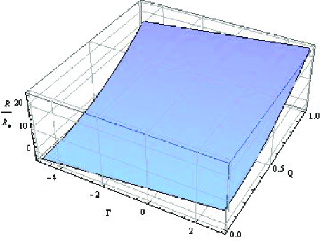
Figure 1: Plot of $\frac{R}{R_{*}}$ for dynamical stability/instability of charged cylinder in Newtonian limit.

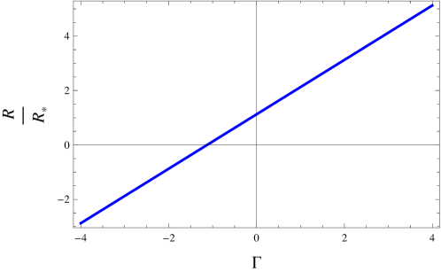
Figure 2: Plot of $\frac{R}{R_{*}}$ for dynamical stability/instability of uncharged cylinder in Newtonian limit.

$$\frac{R}{R_{*}}<\frac{K}{\left[\Gamma+\frac{3}{4}\left(\frac{3}{2}+27Q^{2}\right)\right]},$$ (56)

where $K=\frac{57}{42}$ for the homogeneous cylinder. This means that if $\Gamma$ exceeds $-\frac{3}{4}\left(\frac{3}{2}+27Q^{2}\right)$ by a small amount, the dynamical instability can be prevented till the mass contracts to radius $R_{*}$. The gaseous cylinder remains stable if its radius is larger than $R_{*}$. The ranges of instability for charged homogeneous cylindrical system are shown in Figure 3. It can be seen that the radius of stability is greater than $R_{*}$ for $\Gamma>-1$ in pN limit. We also discuss the criteria and ranges of instability for uncharged cylinder (Figure 4). It is found that $\frac{R}{R_{*}}\geq 0$ when $\Gamma$ exceeds $-\frac{9}{8}$ by a small amount showing stable cylindrical configuration. It is observed that $\Gamma<-1.125$ leads to un-physical results as $\frac{R}{R_{*}}<0$.

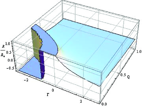
Figure 3: Plot of $\frac{R}{R_{*}}$ for dynamical stability/instability of charged homogeneous cylinder.

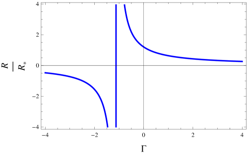
Figure 4: Plot of $\frac{R}{R_{*}}$ for dynamical stability/instability of homogeneous uncharged cylinder.

5 Outlook

This paper is devoted to study the influence of electric charge on dynamical instability of collapsing cylinder. We have followed Eulerian and Lagrangian approaches to find linearized dynamical equations as well as perturbed pressure. This perturbed pressure has been obtained in terms of adiabatic index by taking conservation of baryon numbers. A variational principle has been developed to formulate characteristic frequencies of oscillation which refers to the criteria of dynamical instability for gaseous cylinder. We have also discussed conditions for dynamical instability by taking a homogeneous model for cylinder.

We have computed particular values of radii as well as adiabatic index $\Gamma$ to investigate the marginal stability of homogeneous cylinder (Table 1). It is found that $\Gamma$ takes finite values greater than or equal to $-\frac{3}{4}\left(\frac{3}{2}+27Q^{2}\right)$ for $Q=0.4$ and $q=0.5$ in Newtonian limit. In pN limit, $\frac{R}{R_{*}}$ remains positive for $\Gamma>0$ showing marginal stability of gaseous cylindrical model. We have also discussed the criteria for onset of dynamical instability of gaseous masses.

In Newtonian limit, we have explored the ranges of instability for both charged (Figure 1) as well as uncharged cylinder (Figure 2). There is an extensive literature available for dynamical instability of cylindrical gaseous systems using different techniques in Newtonian limit. Nakamura et al. (1993) studied dynamical instability of self-gravitating cylindrical gaseous cloud by means of normal mode analysis and found unstable solutions against various types of perturbations. Hanawa et al. (1993) discussed fragmentation of cylindrical moleculer cloud with axial magnetic field on the basis of a magnetohydrodynamical stability analysis and found that the presence of magnetic field or rotation shortens the wavelength of most unstable mode. Matsumoto et al. (1994) studied dynamical instability of a self-gravitating magnetized cylindrical cloud by taking rotation around its axis which suffers from various instabilities. Fiege & Pudrit (2000) explored dynamical instability of molecular cylindrical clouds threaded by helical magnetic fields and found that all filamentary molecular clouds initially in equilibrium state cannot be made to undergo radial collapse by increasing the external pressure. Toci & Galli (2015) discussed dynamical instability of cylindrical polytropic filaments and found that the cylindrical polytropes converge at large radii.

In our analysis, the gaseous cylinder remains stable as long as its radius is larger than $R_{*}$ but becomes unstable as its radius contracts to the radius $R_{*}$. For charged cylinder, dynamical instability occurs for smaller values of charge whereas the system becomes stable by increasing charge. The resulting radius of stability is greater than $R_{*}$ for $\Gamma>-\frac{9}{8}$ in case of uncharged cylinder while the dynamical instability occurs for $\Gamma<-1.125$. It is mentioned here that electric charge plays a substantial role to increase stability of cylindrical system as the gaseous mass is more stable in Newtonian limit for larger values of charge.

In pN limit, the gaseous cylinder undergoes dynamical instability if $\Gamma$ exceeds $-\frac{3}{4}\left(\frac{3}{2}+27Q^{2}\right)$ by a small amount. It is found that $\Gamma>-1$ and $Q>0.3$ provide valid ranges of radii for the stability of cylinder whereas only unstable radii exist corresponding to $\Gamma<-1$ and $Q<0.3$ (Figure 3). There is no effect of dissipation on stability of collapsing system in this case. It is worth mentioning here that the gaseous cylinder becomes unstable forever for smaller values of charge. For uncharged cylinder, we have found that $\Gamma$ exceeds $-\frac{9}{8}$ by a small amount showing stable cylindrical configuration (Figure 4). It is observed that $\frac{R}{R_{*}}<0$ for $\Gamma<-1.125$ leading to un-physical results. It is mentioned here that the cylindrical system is more stable in Newtonian limit (Figure 1) for larger values of charge as compared to the post-Newtonian limit (Figure 3). We conclude that the presence of electromagnetic field plays a remarkable role in the emergence of stability of gaseous cylinder.

References

- Ayal et al. (2001) Ayal, S. et al., (2001), Astrophys. J., 550, 846.
- Azam et al. (2016) Azam, M. et al., (2016), Eur. Phys. J. C, 76, 510.
- Chan et al. (1994) Chan, R., Herrera, L., Santos, N.O., (1994), Not. R. Astron. Soc., 267, 637.
- Chandrasekhar (1964) Chandrasekhar, S., (1964), Astrophys. J., 140, 417.
- Chandrasekhar (1965) Chandrasekhar, S., (1965), Astrophys. J., 142, 1519.
- Di Prisco et al. (2009) Di Prisco, A. et al., (2009), Phys. Rev. D, 80, 064031.
- Ghezzi (2005) Ghezzi, C.R., (2005), Phys. Rev. D, 72, 104017.
- Glazer (1976) Glazer, I., (1976), Ann. Phys., 101, 594.
- Herrera et al. (1989) Herrera, L., Le Denmat, G., Santos, N.O., (1989), Not. R. Astron. Soc., 237, 257.
- Marek et al. (2006) Marek, A. et al., (2006), Astron. Astrophys., 445, 273.
- Nunez et al. (2007) Nunez, L.A., Hernandez, H., Abreu, H., (2007), Class. Quantum Grav., 24, 4631.
- Rosseland (1924) Rosseland, S., (1924), Mon. Not. R. Astron. Soc., 84, 720.
- Sharif & Abbas (2011) Sharif, M., Abbas, G., (2011), J. Phys. Soc. Jpn., 80, 104002.
- Sharif & Ahmad (2007) Sharif, M., Ahmad, Z., (2007), Gen. Relativ. Gravit., 39, 1331.
- Sharif & Azam (2012) Sharif, M., Azam, M., (2012), Gen. Relativ. Gravit., 44, 1181.
- Sharif & Azam (2012) Sharif, M., Azam, M., (2012), J. Cosmol. Astropart. Phys., 02, 043.
- Sharif & Azam (2013) Sharif, M., Azam, M., (2013), Mon. Not. R. Astron. Soc., 430, 3048.
- Sharif & Bhatti (2013) Sharif, M., Bhatti, M.Z., (2013), J. Cosmol. Astropart. Phys., 10, 056.
- Sharif & Mumtaz (2016) Sharif, M., Mumtaz, S., (2016), Gen. Relativ. Gravit., 48, 92.
- Stettner (1973) Stettner, R., (1973), Ann. Phys., 80, 212.
- Thorne (1935) Thorne, K.S., (1935), Phys. Rev., 138, B251.
- Nakamura et al. (1993) Nakamura, F., Hanawa, T., Nakano, T., (1993), Astron. Soc. Jpn., 45, 551.
- Hanawa et al. (1993) Hanawa, T. et al., (1993), Astrophys. J., 404, 83.
- Matsumoto et al. (1994) Matsumoto, T. Nakamura, F., Hanawa, T., (1994), arXiv: astro-ph/9405019v1.
- Fiege & Pudrit (2000) Fiege, J.D., Pudrit, R. E., (2000), Mon. Not. R. Astron. Soc., 311, 85.
- Toci & Galli (2015) Toci, C. and Galli, D., (2015), Mon. Not. R. Astron. Soc., 446, 2110.