Requirements for Secure Clock Synchronization

Abstract

This paper establishes a fundamental theory of secure clock synchronization. Accurate clock synchronization is the backbone of systems managing power distribution, financial transactions, telecommunication operations, database services, etc. Some clock synchronization (time transfer) systems, such as the Global Navigation Satellite Systems (GNSS), are based on one-way communication from a master to a slave clock. Others, such as the Network Transport Protocol (NTP), and the IEEE 1588 Precision Time Protocol (PTP), involve two-way communication between the master and slave. This paper shows that all one-way time transfer protocols are vulnerable to replay attacks that can potentially compromise timing information. A set of conditions for secure two-way clock synchronization is proposed and proved to be necessary and sufficient. It is shown that IEEE 1588 PTP, although a two-way synchronization protocol, is not compliant with these conditions, and is therefore insecure. Requirements for secure IEEE 1588 PTP are proposed, and a second example protocol is offered to illustrate the range of compliant systems.

I Introduction

Secure clock synchronization is critical to a host of technologies and infrastructure today. The phasor measurement units (PMUs) that enable monitoring and control in power grids need timing information to synchronize measurements across a wide geographical area [1]. Wireless communication networks synchronize their base stations to enable call handoff [2]. Financial networks transfer time across the globe to ensure a common time for pricing and transaction time-stamping [3]. Cloud database services such as Google’s Cloud Spanner similarly require precise synchronization between the data centers to maintain consistency [4]. These clock synchronization applications have sub-millisecond accuracy and stringent security requirements.

Clock synchronization is performed either by over-the-wire packet-based communication (NTP, PTP, etc.), or by over-the-air radio signals (GNSS [2], cellular signals, LORAN [5], DCF77 [6], etc.); both wired and wireless clock synchronization are used extensively. Synchronization by GNSS is the method of choice in systems with the most stringent accuracy requirements. Equipped with atomic clocks synchronized to the most accurate time standards available, GNSS satellites can synchronize any number of stations on Earth to within a few tens of nanoseconds [7]. NTP is usually only accurate to a few milliseconds, but essentially comes for free whenever the host device is connected to a network.

One-way clock synchronization protocols are based on unidirectional communication from the time master station, A, to the slave station, B. In such protocols, A acts as a broadcast station and may send out timing signals either continuously or periodically. The principal drawback of one-way wireless clock synchronization protocols is their vulnerability to delay attacks in which a man-in-the-middle (MITM) adversary nefariously delays or repeats a valid transmission from one station to another. Cryptographic and other measures can improve the security of one-way protocols against delay and other signal- and data-level spoofing attacks [8, 9, 10], but, as will be shown, such protocols remain fundamentally insecure because of their inability to measure round trip time. They can be secured against unsophisticated attacks, but remain vulnerable to more powerful adversaries.

Two-way clock synchronization protocols involve bi-directional communication between stations A and B. Such protocols enable measurement of the round trip time of the timing signal, which is shown to be necessary for detecting MITM delay attacks. This measurement, however, is not by itself sufficient for provable security against such attacks.

This paper establishes a fundamental theory of secure clock synchronization. In contrast to the current literature on timing security [11, 12, 13, 14, 15, 16, 17], the problem is formalized with definitions, explicit assumptions, and proofs. The major contributions of this work are as follows:

1. One-way synchronization protocols are shown to be insecure against a MITM delay attack. Adversarial delay is shown to be indistinguishable from clock bias, and hence is unobservable without further assumptions.

2. A set of necessary conditions for secure two-way clock synchronization is presented and proved. Similar protocol-specific conditions have been previously proposed [11, 13, 18], but have not been generalized to apply to a universal clock synchronization model.

3. The proposed necessary conditions, with stricter upper bounds, are shown to be sufficient for secure synchronization in presence of a probabilistic polynomial time (PPT) adversary. Provable security for clock synchronization has not previously been explored in the literature.

4. The two-way synchronization scheme of IEEE 1588 PTP is shown to violate a necessary condition for security. This is a known vulnerability of PTP for which a fix has been proposed [11]. Having established a theory for security, this paper is able to show that the proposed fix is sufficient but is not the minimal necessary modification. A more parsimonious security requirement for PTP is presented that is both necessary and sufficient for secure synchronization.

5. A generic construction of a secure two-way clock synchronization protocol is presented to illustrate the general applicability of the proposed necessary and sufficient conditions to a range of underlying protocols.

This paper is a significant extension of [19], by the same authors: (1) the necessary conditions for security have been revamped to incorporate both continuous and packet-based clock synchronization systems, (2) a sufficiency proof for the security conditions has been formulated, and (3) protocol-specific countermeasures presented in the literature have been unified with the proposed conditions.

Wired clock synchronization is inherently more secure than its wireless counterpart because physical access to cables is easier controlled than access to radio channels. This paper primarily focuses on the more challenging task of clock synchronization over a wireless channel; nonetheless, the attacks and security protocols discussed herein also apply to wireline clock synchronization protocols in the case where the adversary gets access to the channel. For example, if an adversary is able to hijack a boundary clock in a wireline PTP network, then the resulting vulnerabilities are equivalent to that of wireless synchronization where the adversary has open access to the radio channel. In fact, an adversarial boundary clock is even more potent than a wireless adversary since it can completely block the authentic signal from reaching B.

The rest of this paper is organized as follows. Previous works on secure clock synchronization, and their relation to this paper, are summarized in Section II. Section III presents a generic model for clock synchronization and shows that all possible one-way synchronization protocols are insecure. Section IV presents the set of security conditions for a wireless clock synchronization protocol, proving these to be necessary by contradiction. Section V presents a proof of sufficiency for the same set of conditions with stricter upper bounds. A construction of an example secure protocol is presented in Section VI, along with the security requirements for IEEE 1588 PTP. Section VII presents a simulation study of a secure clock synchronization model operating over a simplistic channel model. Concluding remarks are made in Section VIII.

II Related Work

GNSS, NTP, and PTP are the most widely used protocols for clock synchronization. A number of research efforts have been made to assess and improve the security of these protocols. This section reviews some of the notable efforts in the literature.

The GNSS jamming and spoofing threat has been recognized in the literature for more than a decade. A survey of the current state-of-the-art in spoofing and anti-spoofing techniques is presented in [8]. Recent works on GNSS anti-spoofing techniques have specifically focused on the case of timing security. Collaborative multi-receiver [16] and direct time estimation [17] techniques have been proposed for robust GNSS clock synchronization.

The growing popularity of IEEE 1588 PTP for synchronization in critical infrastructure has brought about concerns regarding its security [11, 12, 13, 14, 15]. The threats to IEEE 1588 PTP can broadly be categorized into data-level attacks (such as modification of time messages) and physical layer attacks (such as replay and delay attacks). While cryptographic protocols are able to foil data-level attacks against realistic adversaries, some signal-level attacks, such as the delay attack, remain open vulnerabilities. Unfortunately, their execution is relatively simple. Signal-level attacks, such as the man-in-the-middle attack, have been studied in the recent past. However, these studies only include a brief discussion on countermeasure techniques, and no proof or theoretical guarantee of the efficacy of the countermeasures has been provided.

Ullman et al. [11] propose measuring the propagation delays during initialization of clock synchronization and monitoring the propagation delays during the normal operation of the time synchronization protocol. However, [11] does not prove that such a defense would be sufficient to prevent the delay attacks.

In [13], it is remarked that the clock offset computed between multiple master clocks over a symmetric channel must be zero, and thus, if multiple master clocks are available, they can detect any malicious delay introduced by an adversary. However, this defense does not consider the possibility that the adversary may only delay the packets sent to the slave nodes.

The work presented in [18] is perhaps in closest relation to the current paper. Annessi et al. upper bound the clock drift between subsequent synchronization signals using a drift model, and perform two-way exchange of timestamps such that the master clock is able to verify the time at the slave. Furthermore, given the maximum clock drift rate and the maximum and minimum propagation delay of the timing signal, they derive an upper bound on the adversarial delay that can go unnoticed. However, with conservative bounds on the maximum clock drift rate and the variation in path delays, the accuracy guarantees derived in [18] may be insufficient for certain applications. Moreover, as will be shown in this paper, they fail to take account of one the necessary conditions for secure synchronization.

This paper abstracts the clock synchronization model and assesses its security in a generic setting. It is shown that specialization of the generic security conditions to the particular protocols assessed in the aforementioned efforts leads to solutions similar or identical to those previously advanced. Thus, establishing the fundamental theory of secure clock synchronization also serves to unify the prior work in the literature.

III System Model

TABLE I: Notation used in this paper

A	Time master station
B	Time seeker station
$t_{\texttt{m}}^{\texttt{m}_{i}}$	Transmit time, according to m, of its $i$th signal feature
$t_{\texttt{n}}^{\texttt{m}_{i}}$	Receipt time, according to n, of the $i$th signal feature transmitted by m
$\tau_{\texttt{mn}}^{i}$	Delay, in true time, experienced by the $i$th feature in propagating from m to n
$\tau_{\texttt{mn}_{\mathcal{M}}}^{i}$	Component of $\tau_{\texttt{mn}}^{i}$ introduced by the man-in-the-middle adversary
$\tau_{\texttt{mn}_{\mathcal{N}}}^{i}$	Component of $\tau_{\texttt{mn}}^{i}$ due to natural factors, including processing, transmission, and propagation delay
$\bar{\tau}_{\texttt{mn}}^{i}$	Modeled or a priori estimate of $\tau_{\texttt{mn}_{\mathcal{N}}}^{i}$
$\tilde{\tau}_{\texttt{mn}_{\mathcal{N}}}^{i}$	$\tau_{\texttt{mn}_{\mathcal{N}}}^{i}-\bar{\tau}_{\texttt{mn}}^{i}$
$\tau_{\texttt{BB}}$	Delay, in true time, between the receipt of sync and transmission of response at B
$\bar{\tau}_{\texttt{BB}}$	Delay, according to B, between the receipt of sync and transmission of response at B
$\tilde{\tau}_{\texttt{BB}}$	$\tau_{\texttt{BB}}-\bar{\tau}_{\texttt{BB}}$
$\Delta t_{\texttt{AB}}^{i}$	Clock offset between A and B at the time of receipt of the $i$th feature at B
$\Delta\hat{t}_{\texttt{AB}}^{i}$	B’s best estimate of $\Delta t_{\texttt{AB}}^{i}$
$w_{\texttt{mn}}^{i}$	Measurement noise associated with the measured time-of-arrival of the $i$th signal feature from m at n
$\tau_{\rm RTT}^{ij}$	Round trip time, in true time, involving the $i$th and $j$th signal features of A and B, respectively
$\bar{\tau}_{\rm RTT}^{ij}$	Modeled or a priori estimate of $\tau_{\rm RTT}^{ij}$
$z_{\rm RTT}^{ij}$	A noisy measurement of $\tau_{\rm RTT}^{ij}$

A general system model for clock synchronization is shown in Fig. 1. The time seeker station, B, wishes to synchronize its clock to that of the time master station, A. For wireless synchronization applications, stations A and B are assumed to have known locations, $\bm{x}_{\texttt{A}}$ and $\bm{x}_{\texttt{B}}$, respectively. Due to clock imperfections, the time at station B, $t_{\texttt{B}}$, continuously drifts with respect to $t_{\texttt{A}}$, the time at station A. Station B seeks to track the relative drift of its clock by an exchange of signals between A and B. Without loss of generality, this paper assumes $t_{\texttt{A}}$ is equivalent to true time (relative to some reference epoch), a close proxy for which is GPS system time.

It is assumed that A and B are able to exchange cryptographic keys securely, if required. This exchange may occur over a public channel via a protocol such as the Diffie-Hellman key exchange [20] or via quantum key exchange techniques [21, 22]. Alternatively, symmetric keys for neighboring stations may be loaded at the time of installation.

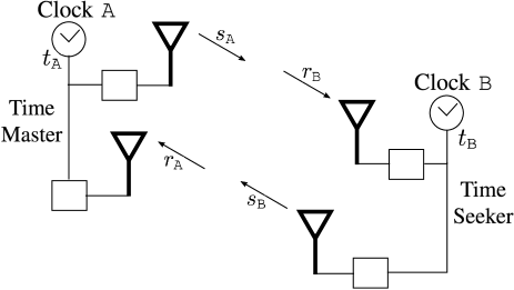
Figure 1: Abstract model of a clock synchronization system with a time master station A and a time seeker station B. The antenna outputs are driven by the clock through the receiver and transmitter blocks.

Station A sends out a sync signal, $s_{\texttt{A}}$, having distinct features which can be disambiguated from one another by observing a window of the signal containing the feature. The transition in $s_{\texttt{A}}$ marking the beginning of a data packet is an example of such a signal feature. Furthermore, the system at A is designed such that the $k$th feature is transmitted at time $t_{\texttt{A}}^{\texttt{A}_{k}}$. B either knows $t_{\texttt{A}}^{\texttt{A}_{k}}$ by prior arrangement, or a digital representation of $t_{\texttt{A}}^{\texttt{A}_{k}}$ is encoded in $s_{\texttt{A}}$ (e.g., a timestamp). In any case, B knows when the $k$th feature was sent, according to A’s clock. This sets up a bijection

$$S_{\texttt{A}}^{k}\rightleftharpoons k\rightleftharpoons t_{\texttt{A}}^{\texttt{A}_{k}}$$ (1)

where $S_{\texttt{A}}^{k}$ represents a window of $s_{\texttt{A}}$ containing the $k$th feature.

Station B’s received sync signal, denoted $r_{\texttt{B}}$, is a delayed and noisy replica of $s_{\texttt{A}}$. Let $\tau_{\texttt{AB}}^{k}$ denote the delay (in true time) experienced by the $k$th feature of $s_{\texttt{A}}$ as it travels from A to B. For line-of-sight (LOS) wireless communication, $\tau_{\texttt{AB}}^{k}$ is the sum of the free-space propagation delay over the distance $\|\bm{x}_{\texttt{B}}-\bm{x}_{\texttt{A}}\|$ and additional delays due to interaction of the timing signal with the intervening channel.

III-A One-Way Clock Synchronization Model

In one-way clock synchronization, the exchange of signals between A and B terminates with reception of the sync signal at B. Let $t_{\texttt{B}}^{\texttt{A}_{k}}$ denote the time according to B at which the $k$th feature of $s_{\texttt{A}}$ is received at B. The window captured by B containing the $k$th feature of $s_{\texttt{A}}$, denoted $R_{\texttt{B}}^{k}$, enables B to measure $t_{\texttt{B}}^{\texttt{A}_{k}}$ to within a small error caused by measurement noise. This error, $w_{\texttt{AB}}^{k}$, is modeled as zero-mean with variance $\sigma_{\epsilon}^{2}$. The measurement itself, denoted $z_{\texttt{B}}^{k}$, is modeled as

$$z_{\texttt{B}}^{k} =t_{\texttt{B}}^{\texttt{A}_{k}}+w_{\texttt{AB}}^{k}$$

$$=t_{\texttt{A}}^{\texttt{A}_{k}}+\tau_{\texttt{AB}}^{k}-\Delta t_{\texttt{AB}}^{k}+w_{\texttt{AB}}^{k}$$ (2)

where

$$\Delta t_{\texttt{AB}}^{k}\equiv t_{\texttt{A}}^{\texttt{A}_{k}}+\tau_{\texttt{AB}}^{k}-t_{\texttt{B}}^{\texttt{A}_{k}}$$ (3)

is the unknown time offset B wishes to estimate. As the bijection in (1) is known to B, B can obtain $t_{\texttt{A}}^{\texttt{A}_{k}}$ for the $k$th detected feature. If a prior estimate $\bar{\tau}_{\texttt{AB}}^{k}$ of the delay $\tau_{\texttt{AB}}^{k}$ is available to B, then the desired time offset can be estimated as

$$\Delta\hat{t}_{\texttt{AB}}^{k} =t_{\texttt{A}}^{\texttt{A}_{k}}+\bar{\tau}_{\texttt{AB}}^{k}-z_{\texttt{B}}^{k}$$ (4)

As a concrete example, consider the case of clock synchronization via GNSS in which B is a GNSS receiver in a known fixed location $\bm{x}_{\texttt{B}}$, and A is a GNSS satellite whose location is known to vary with time as $\bm{x}_{\texttt{A}}(t_{\texttt{A}})$. On detection of the $k$th feature in a window of captured data, B determines $t_{\texttt{A}}^{\texttt{A}_{k}}$ using (1) and also makes the measurement

$$z_{\texttt{B}}^{k} =t_{\texttt{A}}^{\texttt{A}_{k}}+\tau_{\texttt{AB}}^{k}-\Delta t_{\texttt{AB}}^{k}+w_{\texttt{AB}}^{k}$$

$$=t_{\texttt{A}}^{\texttt{A}_{k}}+\left[\frac{\|\bm{x}_{\texttt{B}}-\bm{x}_{\texttt{A}}(t_{\texttt{A}}^{\texttt{A}_{k}})\|+D_{\rho}^{k}}{c}\right]-\Delta t_{\texttt{AB}}^{k}+w_{\texttt{AB}}^{k}$$

where $D_{\rho}^{k}$ is the sum of excess ionospheric and neutral-atmospheric delays (in distance units) and $c$ is the speed of light.

The known receiver and satellite positions can be invoked to model the signal’s propagation delay as

$$\bar{\tau}_{\texttt{AB}}^{k} =\frac{\|\bm{x}_{\texttt{B}}-\bm{x}_{\texttt{A}}(t_{\texttt{A}}^{\texttt{A}_{k}})\|+\bar{D}_{\rho}^{k}}{c}$$

where $\bar{D}_{\rho}^{k}$ is a model of the excess delay $D_{\rho}^{k}$ at the time of receipt of the $k$th feature at B. The modeled excess delay is based on atmospheric models possibly refined by dual-frequency measurements [23]. An estimate of the time offset, $\Delta\hat{t}_{\texttt{AB}}^{k}$, can then be made using $t_{\texttt{A}}^{\texttt{A}_{k}}$, $z_{\texttt{B}}^{k}$, and $\bar{\tau}_{\texttt{AB}}^{k}$ in (4).

It must be noted that, for one-way clock synchronization, any errors in the estimate of the distance between A and B, and in the estimate of the excess channel delay, will appear as an error in the estimate of the time offset.

III-B Two-Way Clock Synchronization Model

As discussed above, if an estimate of $\bar{\tau}_{\texttt{AB}}^{k}$ is available, then clock synchronization is complete after B receives the sync signal $r_{\texttt{B}}$. The response signal from B in a two-way protocol is typically used to either determine, or refine, the estimate of $\bar{\tau}_{\texttt{AB}}^{k}$ with a measurement of the round trip time (RTT). The ability to measure RTT obviates the requirement that $\|\bm{x}_{\texttt{B}}-\bm{x}_{\texttt{A}}\|$ be known a priori. In IEEE 1588 PTP, for example, RTT is measured to initially obtain, and periodically refine, the value of $\bar{\tau}_{\texttt{AB}}^{k}$ used in deriving $\Delta\hat{t}_{\texttt{AB}}^{k}$ from (4).

In the system model considered in this paper, station B transmits a response $s_{\texttt{B}}$ that is designed such that (1) there is a one-to-one mapping $l(k)$ between the $l$th feature in $s_{\texttt{B}}$ and the $k$th feature in $s_{\texttt{A}}$, and (2) the $l$th feature’s index can be inferred by observation of a window containing it. Symbolically, if $S_{\texttt{B}}^{l}$ is a window of $s_{\texttt{B}}$ containing the $l$th feature of the response signal, then

$$S_{\texttt{B}}^{l}\rightleftharpoons l(k)\rightleftharpoons k$$ (5)

On receipt of the $k$th feature in $s_{\texttt{A}}$, at time $t_{\texttt{B}}^{\texttt{A}_{k}}$ by B’s clock, but at $z_{\texttt{B}}^{k}$ as measured by B, B transmits the $l$th feature in $s_{\texttt{B}}$ after a short delay, $\tau_{\texttt{BB}}$ (in true time), hereon referred to as the layover time.

The layover time is introduced as a practical consideration. On receipt of A’s $k$th feature, B is physically unable to transmit its own $l$th feature with zero delay. Thus, B is allowed to specify a short layover time, $\bar{\tau}_{\texttt{BB}}$, after which it intends to launch its $l$th feature. It is important to note that the actual layover time, $\tau_{\texttt{BB}}$, will not be the same as the intended layover time due to (1) non-zero measurement noise $w_{\texttt{AB}}^{k}$ and (2) non-zero frequency offset of the clock at B with respect to true time. However, if the layover time is sufficiently short and the measurement noise is benign, the difference $\bar{\tau}_{\texttt{BB}}-\tau_{\texttt{BB}}$ can be made negligible compared to the time synchronization requirement, with the actual value depending on the quality of B’s clock.

Station A receives the response signal as a delayed and noisy replica of $s_{\texttt{B}}$, denoted $r_{\texttt{A}}$. The delay experienced by the $l$th feature as it travels from B to A, in true time, is denoted $\tau_{\texttt{BA}}^{l}$. Station A captures a window $R_{\texttt{A}}^{l}$ of $r_{\texttt{A}}$ that enables A to identify the $l$th feature in $s_{\texttt{B}}$ according to (5), and to infer that the received feature is in response to the $k$th feature transmitted by A. Furthermore, A makes a noise-corrupted measurement $z_{\texttt{A}}^{l}$ of the time-of-arrival of the $l$th feature in $s_{\texttt{B}}$, according to A’s clock. The noise, denoted $w_{\texttt{BA}}^{l}$, is again modeled as zero-mean with variance $\sigma_{\epsilon}^{2}$. The full measurement model is given by

$$z_{\texttt{A}}^{l} =t_{\texttt{A}}^{\texttt{B}_{l}}+w_{\texttt{BA}}^{l}$$

$$=t_{\texttt{A}}^{\texttt{A}_{k}}+\tau_{\texttt{AB}}^{k}+\tau_{\texttt{BB}}+\tau_{\texttt{BA}}^{l}+w_{\texttt{BA}}^{l}$$

Since $t_{\texttt{A}}^{\texttt{A}_{k}}$ is exactly known at A, a direct noisy measurement of the round trip time $\tau_{\texttt{AB}}^{k}+\tau_{\texttt{BB}}+\tau_{\texttt{BA}}^{l}$ can be made as

$$z_{\rm RTT}^{kl}\equiv z_{\texttt{A}}^{l}-t_{\texttt{A}}^{\texttt{A}_{k}}$$ (6)

Note that the noise $w_{\texttt{BA}}^{l}$ and $w_{\texttt{AB}}^{k}$ in $z_{\rm RTT}^{kl}$ is embedded within $z_{\texttt{A}}^{l}$ and $\tau_{\texttt{BB}}$, respectively. Under the assumption of symmetric delays, i.e., $\tau_{\texttt{AB}}^{k}=\tau_{\texttt{BA}}^{l}$, and with knowledge of $\bar{\tau}_{\texttt{BB}}$, the measured RTT in (6) can be exploited to improve the modeled propagation delay for future exchanges between A and B:

$$\bar{\tau}_{\texttt{AB}}^{m}=\bar{\tau}_{\texttt{BA}}^{n}=\frac{z_{\rm RTT}^{kl}-\bar{\tau}_{\texttt{BB}}}{2}$$

where $m>k$ and $n>l$.

The two-way exchange of sync and response messages is summarized visually in Fig. 2.

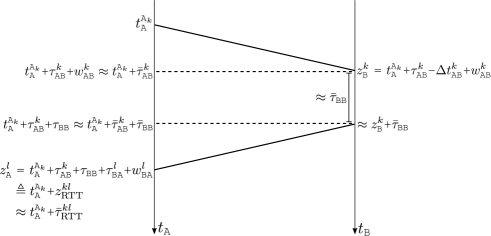
Figure 2: Two-way exchange of sync and response messages between A and B in the absence of a man-in-the-middle adversary.

Since RTT will play a central role in the discussion on secure synchronization later on, various definitions and assumptions concerning RTT are stated here for clarity:

• RTT for the $k$th feature in $s_{\texttt{A}}$ and the corresponding $l$th feature in $s_{\texttt{B}}$ is defined as

  $$\tau_{\rm RTT}^{kl}\equiv\tau_{\texttt{AB}}^{k}+\tau_{\texttt{BB}}+\tau_{\texttt{BA}}^{l}$$

• Measured RTT includes, in addition to RTT, measurement noise at A; it is modeled as

  $$z_{\rm RTT}^{kl}=\tau_{\texttt{AB}}^{k}+\tau_{\texttt{BB}}+\tau_{\texttt{BA}}^{l}+w_{\texttt{BA}}^{l}$$

• Modeled RTT, also called the prior estimate of RTT, is defined as

  $$\bar{\tau}_{\rm RTT}^{kl}\equiv\bar{\tau}_{\texttt{AB}}^{k}+\bar{\tau}_{\texttt{BB}}+\bar{\tau}_{\texttt{BA}}^{l}$$ (7)

  For example, in the case of wireless clock synchronization with LOS electromagnetic signals, a prior estimate of RTT is based on the distance between A and B and on models of channel delays in excess of free-space propagation between these.

• The modeled RTT, $\bar{\tau}_{\rm RTT}^{kl}$, can be refined with measurements of RTT in a two-way protocol. Alternatively, as will be discussed later, if an accurate modeled RTT is available, it and the measured RTT can be used to detect delay attacks.

• Unambiguous measurement of RTT requires that there exist a one-to-one mapping between the signal features in $s_{\texttt{A}}$ and $s_{\texttt{B}}$, as mathematically represented in (5). On detection of the $l$th feature in $s_{\texttt{B}}$, A must be able to deduce that this feature was transmitted approximately $\bar{\tau}_{\texttt{BB}}$ after B received the $k$th feature in $s_{\texttt{A}}$. This requirement is appropriately a part of the RTT definition since it enables A to unambiguously measure RTT.

III-C Attack Model

The attack model in this paper considers a MITM adversary $\mathcal{M}$. The available computational resources allow $\mathcal{M}$ to execute probabilistic polynomial time (PPT) algorithms. $\mathcal{M}$ can receive, detect, and replay signals from A and B with arbitrarily precise directional antennas. Additionally, $\mathcal{M}$ has precise knowledge of $\bm{x}_{\texttt{A}}$ and $\bm{x}_{\texttt{B}}$, and can take up any position around or between the two stations. It has unrestricted access to the signals that A and B exchange over the air, and has complete knowledge of their synchronization protocol save for the cryptographic keys.

Let $L$ denote the alert limit, defined as the error in time synchronization not to be exceeded without issuing an alert.

Definition III.1.

Clock synchronization is defined to be compromised if ${|\Delta t_{\texttt{AB}}-\Delta\hat{t}_{\texttt{AB}}|\geq L}$.

Note that, in the absence of an adversary, clock synchronization is not compromised so long as

$$|\tau_{\texttt{AB}}^{k}-\bar{\tau}_{\texttt{AB}}^{k}+w_{\texttt{AB}}^{k}|<L$$

However, in the presence of a MITM adversary, the sync signal is delayed or advanced such that

$$\tau_{\texttt{AB}}^{k}=\tau_{\texttt{AB}_{\mathcal{N}}}^{k}+\tau_{\texttt{AB}_{\mathcal{M}}}^{k}$$ (8)

where $\tau_{\texttt{AB}_{\mathcal{N}}}^{k}>0$ is the natural or physical delay (equal to $\tau_{\texttt{AB}}^{k}$ in the absence of an adversary) and $\tau_{\texttt{AB}_{\mathcal{M}}}^{k}\geq 0$ is the adversarial delay. In this case, if

$$|\tau_{\texttt{AB}}^{k}-\bar{\tau}_{\texttt{AB}}^{k}+w_{\texttt{AB}}^{k}|=|\tau_{\texttt{AB}_{\mathcal{N}}}^{k}-\bar{\tau}_{\texttt{AB}}^{k}+\tau_{\texttt{AB}_{\mathcal{M}}}^{k}+w_{\texttt{AB}}^{k}|\geq L$$ (9)

then clock synchronization is compromised.

III-D Vulnerability of One-Way Clock Synchronization

One-way clock synchronization is fundamentally vulnerable to a delay attack because it provides no mechanism to measure RTT. The adversary $\mathcal{M}$ can compromise any one-way wireless clock synchronization protocol by retransmitting the authentic sync signal from A such that the retransmitted signal, $s_{\mathcal{M}}$, overpowers or otherwise supersedes the authentic signal $s_{\texttt{A}}$. In the absence of additional assumptions beyond those underpinning the one-way protocol described earlier, $\mathcal{M}$ can introduce an arbitrary delay $\tau_{\texttt{AB}_{\mathcal{M}}}^{k}$ in its retransmission, thereby compromising the synchronization process.

Note that whereas counterfeit signal attacks can be prevented by authentication and cryptographic methods [24], these techniques do not prevent delay attacks because the delayed or repeated signal has the same cryptographic characteristics as that of the genuine signal, the only difference being that it is received with a (possibly small) additional delay.

The delay introduced by $\mathcal{M}$ is added to the natural delay, $\tau_{\texttt{AB}_{\mathcal{N}}}^{k}$, of the signal between A and B. As a result, an error of $\approx\tau_{\texttt{AB}_{\mathcal{M}}}^{k}$ is introduced in the estimated time offset at B. From (4), it follows that

$$\Delta\hat{t}_{\texttt{AB}}^{k} =t_{\texttt{A}}^{\texttt{A}_{k}}+\bar{\tau}_{\texttt{AB}}^{k}-z_{\texttt{B}}^{k}$$

$$=t_{\texttt{A}}^{\texttt{A}_{k}}+\bar{\tau}_{\texttt{AB}}^{k}-(t_{\texttt{A}}^{\texttt{A}_{k}}+\tau_{\texttt{AB}}^{k}-\Delta t_{\texttt{AB}}^{k}+w_{\texttt{AB}}^{k})$$

$$=(\bar{\tau}_{\texttt{AB}}^{k}-\tau_{\texttt{AB}_{\mathcal{N}}}^{k})-\tau_{\texttt{AB}_{\mathcal{M}}}^{k}+\Delta t_{\texttt{AB}}^{k}-w_{\texttt{AB}}^{k}$$

$$\approx\Delta t_{\texttt{AB}}^{k}-\tau_{\texttt{AB}_{\mathcal{M}}}^{k}$$ (10)

where it is assumed that the error due to inaccurately modeled delay is negligible and that $\sigma_{\epsilon}\ll\tau_{\texttt{AB}_{\mathcal{M}}}^{k}$. In the absence of an RTT measurement, and without further assumptions on the nature of the protocol or the clock drift model considered, the adversarial delay $\tau_{\texttt{AB}_{\mathcal{M}}}$ is indistinguishable from a clock offset of the same magnitude.

To be sure, measures can be taken to make a MITM delay attack harder to execute without detection. But, importantly, these measures cannot guarantee that the synchronization will remain uncompromised. Various measures proposed in the literature, and their shortcomings, are discussed below.

Received Signal Strength Monitoring

The adversary $\mathcal{M}$ might attempt to overpower the authentic signal in order to spoof the sync message, leading to an increase in the total signal power received at B. Station B could monitor the received signal strength (RSS) to detect such an attack [25]. However, a potent adversary could transmit, in addition to its delayed signal, an amplitude-matched, phase-inverted nulling signal that annihilates the authentic sync signal $s_{\texttt{A}}$ as received at B, thus preventing an unusual increase in received power at B. If $\mathcal{M}$ is positioned along the straight-line path between A and B, nulling of $s_{\texttt{A}}$ can be effected without prior knowledge of $s_{\texttt{A}}$. A laboratory demonstration of such nulling is reported in [26].

Selective Rejection of False Signal

If B receives both the authentic and false (delayed) sync signals, it may be able to apply angle-of-arrival or signal processing techniques to selectively reject the delayed signal [8, 9, 27, 28]. However, discrimination based on angle-of-arrival fails if $\mathcal{M}$ is positioned along the line from A to B, and, as conceded in [9], signal-processing-based techniques for selective rejection of false signals can be thwarted by an adversary transmitting an additional nulling signal, as described above.

Collaborative Verification

Multiple time seekers may attempt to synchronize to the same time master. In this scenario, the time seekers can potentially detect malicious activity by cross-checking the received signals [16]. In the simplest implementation, all time seekers can collaborate to verify that they are synchronized amongst each other. In case of an uncoordinated attack against a subset of time seekers, this verification would expose the attack since the time offset computed at the attacked subset would be different from that computed at the other stations. In principle, however, it is possible for an adversary to execute a coordinated attack against all the time seekers, thus concealing its presence.

IV Necessary Conditions for Secure Synchronization

This section presents a set of conditions for secure two-way clock synchronization and proves these to be necessary by contradiction. In other words, it is shown that if a two-way clock synchronization protocol does not satisfy any one of these proposed conditions, there exists an attack that can compromise clock synchronization without detection.

It is important to note that the ability to measure RTT in a two-way protocol is necessary, but not sufficient, for provably secure synchronization. As an example, IEEE 1588 PTP is a two-way protocol that has been proposed as an alternative to GNSS for sub-microsecond clock synchronization in critical infrastructure such as the PMU network. But, despite the bi-directional exchange between stations, and hence the ability to measure RTT, recent work has shown that PTP is vulnerable to delay attacks in which a MITM introduces asymmetric delay between A and B. Asymmetric delay breaks the assumption that $\tau_{\texttt{AB}}^{k}=\tau_{\texttt{BA}}^{k}$ and leads to an erroneous prior for $\bar{\tau}_{\texttt{AB}}$ and $\bar{\tau}_{\texttt{BA}}$ for future exchanges. This vulnerability is documented in both the literature [11, 13, 18] and the IEEE 1588-2008 standard. Thus, a secure two-way clock synchronization protocol must satisfy additional security requirements beyond the ability to measure RTT.

The conditions introduced below are not tied to any specific protocol, unlike some measures proposed in the current literature [11, 12, 13, 14, 15, 16, 17]. They are generally applicable to any two-way protocol (e.g., PTP) for which the foregoing two-way synchronization model applies.

Assuming the time master A initiates the two-way communication, the necessary conditions for secure clock synchronization are as follows:

1. Both A and B must transmit unpredictable waveforms to prevent the adversary $\mathcal{M}$ from generating counterfeit signals that pass authentication. In practice, this implies the use of a cryptographic construct such as a message authentication code (MAC) or a digital signature.

2. The propagation time of the signal must be irreducible to within the alert limit $L$ along both signal paths. For wireless clock synchronization, this condition implies synchronization via LOS electromagnetic signals as $L\rightarrow 0$.

3. The RTT between A and B must be known to A and measurable by A to within the alert limit $L$. The RTT must include the delays internal to both A and B, in addition to the propagation delay. Station A must know of any intentional delay introduced by B, such as the layover time $\tau_{\texttt{BB}}$ introduced earlier.

IV-A Proof of Necessity of Conditions

IV-A1 Stations A and B must transmit unpredictable signals

To prove this condition is necessary, two scenarios are considered: a) station A transmits a signal waveform $s_{\texttt{A}}$ that is predictable, and, b) station B transmits a signal waveform $s_{\texttt{B}}$ that is predictable.

$s_{\texttt{A}}$ is predictable

$\mathcal{M}$ can compromise synchronization without detection as follows:

1. $\mathcal{M}$ takes up a position between A and B along the line joining the antennas at the two stations.

2. $\mathcal{M}$ initially transmits a replica of $s_{\texttt{A}}$ such that B receives identical signals from both A and $\mathcal{M}$. Subsequently, $\mathcal{M}$ increases its signal power or otherwise supersedes $s_{\texttt{A}}$ (e.g., via signal nulling, as discussed earlier) such that B tracks $s_{\mathcal{M}}$, the signal transmitted by $\mathcal{M}$. (Hereafter, whenever signals from $\mathcal{M}$ compete with those from A or B, it will be assumed that those from $\mathcal{M}$ exert control.)

3. Exploiting the predictability of $s_{\texttt{A}}$, $\mathcal{M}$ advances its replica $s_{\mathcal{M}}$ with respect to $s_{\texttt{A}}$ by $|\tau_{\texttt{AB}_{\mathcal{M}}}^{k}|$, where $\tau_{\texttt{AB}_{\mathcal{M}}}^{k}<0$. B tracks the advanced signal, resulting in an error of $\tau_{\texttt{AB}_{\mathcal{M}}}^{k}$ in the computed $\Delta\hat{t}_{\texttt{AB}}^{k}$ as shown in (10).

4. B transmits the unpredictable response $s_{\texttt{B}}$ compliant with the prearranged layover time $\bar{\tau}_{\texttt{BB}}$. $\mathcal{M}$ intercepts this signal from B, and replays it to A with a delay of $\tau_{\texttt{BA}_{\mathcal{M}}}^{l}=-\tau_{\texttt{AB}_{\mathcal{M}}}^{k}>0$, causing A to track the delayed signal. As a result, the RTT is $\tau_{\texttt{AB}}^{k}+\tau_{\texttt{BB}}+\tau_{\texttt{BA}}^{l}$ as A expects. In summary:

   $$\tau_{\texttt{AB}}^{k} =\tau_{\texttt{AB}_{\mathcal{N}}}^{k}+\tau_{\texttt{AB}_{\mathcal{M}}}^{k}$$

   $$\tau_{\texttt{BA}}^{l} =\tau_{\texttt{BA}_{\mathcal{N}}}^{l}+\tau_{\texttt{BA}_{\mathcal{M}}}^{l}=\tau_{\texttt{BA}_{\mathcal{N}}}^{l}-\tau_{\texttt{AB}_{\mathcal{M}}}^{k}$$

   $$\Rightarrow\tau_{\texttt{AB}}^{k}+\tau_{\texttt{BA}}^{l} =\tau_{\texttt{AB}_{\mathcal{N}}}^{k}+\tau_{\texttt{BA}_{\mathcal{N}}}^{l}$$

   Thus, $\mathcal{M}$ undoes the effect of its sync advance, preventing A from detecting the attack.

$s_{\texttt{B}}$ is predictable

$\mathcal{M}$ can compromise synchronization without detection by replicating B’s behavior:

1. $\mathcal{M}$ takes up a position between A and B along the line joining the antennas at the two stations.

2. $\mathcal{M}$ receives the sync signal and generates a valid response with a delay

   $$\bar{\tau}_{\texttt{BB}}+\frac{\|\bm{x}_{\mathcal{M}}-\bm{x}_{\texttt{B}}\|}{\|\bm{x}_{\texttt{A}}-\bm{x}_{\texttt{B}}\|}\left(\bar{\tau}_{\texttt{AB}}^{k}+\bar{\tau}_{\texttt{BA}}^{l}\right)$$ (11)

   such that the RTT is $\bar{\tau}_{\texttt{AB}}^{k}+\bar{\tau}_{\texttt{BB}}+\bar{\tau}_{\texttt{BA}}^{l}$, as A expects.

3. $\mathcal{M}$ records the unpredictable signal from A and replays it to B with an arbitrary delay $\tau_{\texttt{AB}_{\mathcal{M}}}^{k}>0$. This results in an error of approximately $\tau_{\texttt{AB}_{\mathcal{M}}}^{k}$ in the computed $\Delta\hat{t}_{\texttt{AB}}^{k}$ at B, as shown in (10).

IV-A2 Propagation time must be irreducible to within $L$

If there exists a channel that reduces the propagation time from A to B or from B to A by more than $L$ as compared to the channel used by A and B, then $\mathcal{M}$ can compromise synchronization without detection. The following attack assumes the propagation time from A to B is reducible by more than $L$; a similar attack exploits the situation in which the propagation time from B to A is reducible by more than $L$.

1. $\mathcal{M}$ records the sync signal $s_{\texttt{A}}$ going from A to B.

2. $\mathcal{M}$ makes the recorded signal reach B advanced by $|\tau_{\texttt{AB}_{\mathcal{M}}}^{k}|$ compared to $s_{\texttt{A}}$, where $\tau_{\texttt{AB}_{\mathcal{M}}}^{k}<-L$. An error of $\tau_{\texttt{AB}_{\mathcal{M}}}^{k}$ is introduced in the time offset value computed at B as shown in (10).

3. $\mathcal{M}$ records the response signal $s_{\texttt{B}}$, which has the expected prearranged layover time $\tau_{\texttt{BB}}\approx\bar{\tau}_{\texttt{BB}}$. $\mathcal{M}$ replays this signal to A with a delay of $\tau_{\texttt{BA}_{\mathcal{M}}}^{l}=-\tau_{\texttt{AB}_{\mathcal{M}}}^{k}$ such that the RTT is consistent with what A expects.

IV-A3 RTT known to and measurable by A to within $L$

Synchronization can be compromised without detection if $|z_{\rm RTT}^{kl}-\bar{\tau}_{\rm RTT}^{kl}|>L$ with non-negligible probability even in the absence of an adversary. This condition can be met if a) the prior estimates $\bar{\tau}_{\texttt{AB}}^{k}$, $\bar{\tau}_{\texttt{BA}}^{l}$, or $\bar{\tau}_{\texttt{BB}}$ are not accurate to the corresponding true values to within $L$, or b) the magnitude of the measurement error sum $|w_{\texttt{AB}}^{k}+w_{\texttt{BA}}^{l}|$ is larger than $L$. Note that the condition $|w_{\texttt{AB}}^{k}|>L$ compromises synchronization even absent an adversary. An adversary $\mathcal{M}$ can exploit the condition $|z_{\rm RTT}^{kl}-\bar{\tau}_{\rm RTT}^{kl}|>L$ as follows:

1. $\mathcal{M}$ initially transmits a replica of $s_{\texttt{A}}$ such that B receives identical signals from both A and $\mathcal{M}$. Subsequently, $\mathcal{M}$ introduces a delay $\tau_{\texttt{AB}_{\mathcal{M}}}^{k}>0$ in the replayed signal $s_{\mathcal{M}}$. As assumed earlier, $s_{\mathcal{M}}$ exerts control and introduces an error of approximately $\tau_{\texttt{AB}_{\mathcal{M}}}^{k}$ in the computed $\Delta\hat{t}_{\texttt{AB}}^{k}$ at B, as shown in (10).

2. Station B transmits the response signal with the prearranged layover time $\tau_{\texttt{BB}}\approx\bar{\tau}_{\texttt{BB}}$ with respect to the delayed signal.

3. In the received signal $r_{\texttt{A}}$, A identifies the expected feature $l(k)$. The RTT, if measurable, includes the delay $\tau_{\texttt{AB}_{\mathcal{M}}}^{k}$ introduced by $\mathcal{M}$.

4. However, A is unable to definitively declare an attack, since the errors in the modeled RTT and/or the measurement of RTT are possibly larger than $L$. In other words, it is not possible to claim that $|z_{\rm RTT}^{kl}-\bar{\tau}_{\rm RTT}^{kl}|>L$ only in the presence of adversarial delay.

V Proof of Sufficiency

This section presents a sufficiency proof for the set of security conditions proposed in the previous section. A sufficiency proof guarantees secure synchronization under the considered system and attack models. This paper draws inspiration from the literature on modern cryptography and formalizes the problem of secure clock synchronization with explicit definitions, assumptions, and proofs.

V-A Assumptions

This proof assumes that the system under consideration strictly complies with the set of necessary security conditions. Specifically,

1. Both A and B use an authenticated encryption scheme to generate unpredictable and verifiably authentic signals in the presence of a probabilistic polynomial time (PPT) adversary.

2. The difference between the RTT along the communication channel between A and B and the shortest possible RTT is negligible as compared to $L$.

3. The difference between the modeled delays $\bar{\tau}_{\texttt{AB}}^{k}$ and $\bar{\tau}_{\texttt{BA}}^{l}$ and the true delays $\tau_{\texttt{AB}}^{k}$ and $\tau_{\texttt{BA}}^{l}$, respectively, is negligible as compared to $L$.

   $$|\bar{\tau}_{\texttt{AB}}^{k}-\tau_{\texttt{AB}_{\mathcal{N}}}^{k}|\ll L$$ (12)

   and

   $$|\bar{\tau}_{\texttt{BA}}^{l}-\tau_{\texttt{BA}_{\mathcal{N}}}^{l}|\ll L$$ (13)

   Furthermore, A and B agree upon a fixed layover time $\bar{\tau}_{\texttt{BB}}$, and the difference between this and the true layover time is negligible: $|\tau_{\texttt{BB}}-\bar{\tau}_{\texttt{BB}}|\ll L$.

4. The standard deviation of the noise corrupting the measurements $t_{\texttt{B}}^{\texttt{A}_{k}}$ and $t_{\texttt{A}}^{\texttt{B}_{l}}$ is negligible compared to the alert limit:

   $$\sigma_{\epsilon}\ll L$$ (14)

Notice that the above assumptions are the same as the necessary conditions in Section IV, but with stricter upper bounds on the conditions.

If symmetric keys are exchanged prior to synchronization, then private-key cryptographic schemes such as Encrypt-then-MAC [29] can be used for authenticated encryption. Alternatively, if the keys must be exchanged over a public channel, then digital signatures [30] can be used to authenticate the encrypted messages. Cryptographic authentication schemes like MAC and digital signatures generate a tag associated with a message. Qualitatively, a MAC or digital signature scheme is secure if a PPT adversary, even when given access to multiple valid message-tag pairs of its own choice (as many as possible in polynomial time), cannot generate a valid tag for a new message with non-negligible probability. Irrespective of the cryptographic scheme used, this proof assumes that the probability of $\mathcal{M}$ generating a new valid sync or response signal is a negligible function of the key length $n$:

$$\mathbb{P}\left[\mathsf{Valid}\right]<\mathsf{negl}(n)$$ (15)

To detect an attack before the synchronization error exceeds $L$, A must select a threshold lower than $L$ beyond which an attack is declared. Consider the modeled RTT, $\bar{\tau}_{\rm RTT}^{kl}$, as defined in (7), and the measurement $z_{\rm RTT}^{kl}$ as defined in (6). A threshold less than $L$, say $L-\delta$ with $0<\delta<L$, is set by station A such that if $|z_{\rm RTT}^{kl}-\bar{\tau}_{\rm RTT}^{kl}|>L-\delta$, then an attack is declared.

V-B Definitions

Definition V.1.

A PPT adversary $\mathcal{M}$ succeeds if clock synchronization is compromised (Definition III.1) and

$$|z_{\rm RTT}^{kl}-\bar{\tau}_{\rm RTT}^{kl}|\leq L-\delta$$

Definition V.2.

Faster-than-light (superluminal) propagation is defined to be hard if $\mathcal{M}$ cannot propagate a signal at a speed higher than the speed of light with non-negligible probability. Under hardness of superluminal propagation

$$\mathbb{P}[\mathsf{Superluminal}]\approx 0$$

Definition V.3.

A clock synchronization protocol is defined to be secure if, under the hardness of superluminal propagation assumption,

$$\mathbb{P}[\mathsf{Success}]<\mathsf{negl}(n)$$

where $\mathsf{Success}$ for $\mathcal{M}$ is defined in Definition V.1.

V-C Proof

In the presence of an adversary $\mathcal{M}$, the measurement $z_{\rm RTT}^{kl}$ is modeled as

$$z_{\rm RTT}^{kl} =\tau_{\texttt{AB}_{\mathcal{N}}}^{k}+\tau_{\texttt{AB}_{\mathcal{M}}}^{k}+\tau_{\texttt{BA}_{\mathcal{N}}}^{l}+\tau_{\texttt{BA}_{\mathcal{M}}}^{l}+\tau_{\texttt{BB}}+w_{\texttt{BA}}^{l}$$ (16)

Let $\tilde{\tau}_{\texttt{AB}_{\mathcal{N}}}^{k}$ and $\tilde{\tau}_{\texttt{BA}_{\mathcal{N}}}^{l}$ denote the error in the modeled signal delay due to natural/physical phenomenon. Also, let $\tilde{\tau}_{\texttt{B}}$ be the difference between the intended layover time $\bar{\tau}_{\texttt{BB}}$ and the actual layover time $\tau_{\texttt{BB}}$. Note that these might be positive or negative.

$$\tilde{\tau}_{\texttt{AB}_{\mathcal{N}}}^{k} =\tau_{\texttt{AB}_{\mathcal{N}}}^{k}-\bar{\tau}_{\texttt{AB}}^{k}$$ (17)

$$\tilde{\tau}_{\texttt{BA}_{\mathcal{N}}}^{l} =\tau_{\texttt{BA}_{\mathcal{N}}}^{l}-\bar{\tau}_{\texttt{BA}}^{l}$$ (18)

$$\tilde{\tau}_{\texttt{BB}} =\tau_{\texttt{BB}}-\bar{\tau}_{\texttt{BB}}$$ (19)

From (7), (16), (17), (18), and (19) it follows that

$$z_{\rm RTT}^{kl} =\bar{\tau}_{\rm RTT}^{kl}+\tilde{\tau}_{\texttt{AB}_{\mathcal{N}}}^{k}+\tau_{\texttt{AB}_{\mathcal{M}}}^{k}+\tilde{\tau}_{\texttt{BA}_{\mathcal{N}}}^{l}+\tau_{\texttt{BA}_{\mathcal{M}}}^{l}+\tilde{\tau}_{\texttt{BB}}+w_{\texttt{BA}}^{l}$$

Following the assumptions in (12) and (13), the residual delays are negligible in comparison to $L$:

$$|\tilde{\tau}_{\texttt{AB}_{\mathcal{N}}}^{k}| \ll L$$ (20)

$$|\tilde{\tau}_{\texttt{BA}_{\mathcal{N}}}^{l}| \ll L$$ (21)

This assumption is reasonable since otherwise the system could not confidently meet the accuracy requirements even in the absence of an adversary. Also, if $\bar{\tau}_{\texttt{BB}}$ is a short time interval and the measurement noise $\sigma_{\epsilon}$ is benign, it is reasonable to assume that

$$|\tilde{\tau}_{\texttt{BB}}|\ll L$$ (22)

Note that $\mathcal{M}$ can advance the signal by (a) forging a valid message/tag pair, or (b) propagating the signal faster-than-light. The assumptions of secure MAC and hardness of superluminal propagation enforce that

$$\mathbb{P}[\tau_{\texttt{AB}_{\mathcal{M}}}^{k}<0] <\mathbb{P}[\mathsf{Valid}]+\mathbb{P}[\mathsf{Superluminal}]$$

$$\approx\mathsf{negl}(n)$$

In order to stay undetected, the adversary must ensure

$$L-\delta \geq|z_{\rm RTT}^{kl}-\bar{\tau}_{\rm RTT}^{kl}|$$

$$=|\tilde{\tau}_{\texttt{AB}_{\mathcal{N}}}^{k}+\tau_{\texttt{AB}_{\mathcal{M}}}^{k}+\tilde{\tau}_{\texttt{BA}_{\mathcal{N}}}^{l}+\tau_{\texttt{BA}_{\mathcal{M}}}^{l}+\tilde{\tau}_{\texttt{BB}}+w_{\texttt{BA}}^{l}|$$ (23)

At the same time, in order to compromise time transfer, from (9), $\mathcal{M}$ must ensure

$$L \leq|\tilde{\tau}_{\texttt{AB}_{\mathcal{N}}}^{k}+\tau_{\texttt{AB}_{\mathcal{M}}}^{k}+w_{\texttt{AB}}^{k}|$$

$$\leq|\tilde{\tau}_{\texttt{AB}_{\mathcal{N}}}^{k}+w_{\texttt{AB}}^{k}|+|\tau_{\texttt{AB}_{\mathcal{M}}}^{k}|$$

$$\Rightarrow|\tau_{\texttt{AB}_{\mathcal{M}}}^{k}| \geq L-|\tilde{\tau}_{\texttt{AB}_{\mathcal{N}}}^{k}+w_{\texttt{AB}}^{k}|$$ (24)

The probability of success for $\mathcal{M}$ is evaluated as

$$\mathbb{P}[\mathsf{Success}] =\mathbb{P}[(\mathsf{Success})\cap(\tau_{\texttt{AB}_{\mathcal{M}}}^{k}<0)]+$$

$$\qquad\qquad\mathbb{P}[(\mathsf{Success})\cap(\tau_{\texttt{AB}_{\mathcal{M}}}^{k}\geq 0)]$$

$$=\mathbb{P}[(\mathsf{Success})|(\tau_{\texttt{AB}_{\mathcal{M}}}^{k}<0)]\mathbb{P}[\tau_{\texttt{AB}_{\mathcal{M}}}^{k}<0]+$$

$$\qquad\qquad\mathbb{P}[(\mathsf{Success})\cap(\tau_{\texttt{AB}_{\mathcal{M}}}^{k}\geq 0)]$$

$$\leq\mathbb{P}[\tau_{\texttt{AB}_{\mathcal{M}}}^{k}<0]+\mathbb{P}[(\mathsf{Success})\cap(\tau_{\texttt{AB}_{\mathcal{M}}}^{k}\geq 0)]$$

$$<\mathsf{negl}(n)+\mathbb{P}[(\mathsf{Success})\cap(\tau_{\texttt{AB}_{\mathcal{M}}}^{k}\geq 0)]$$ (25)

In the case where $\tau_{\texttt{AB}_{\mathcal{M}}}\geq 0$, (24) simplifies to

$$\tau_{\texttt{AB}_{\mathcal{M}}}^{k}\geq L-|\tilde{\tau}_{\texttt{AB}_{\mathcal{N}}}^{k}+w_{\texttt{AB}}^{k}|$$

Substituting the least possible value of $\tau_{\texttt{AB}_{\mathcal{M}}}^{k}$ into (23), it follows that

$$|\tilde{\tau}_{\texttt{AB}_{\mathcal{N}}}^{k}+L-|\tilde{\tau}_{\texttt{AB}_{\mathcal{N}}}^{k}+w_{\texttt{AB}}^{k}|+\tilde{\tau}_{\texttt{BA}_{\mathcal{N}}}^{l}+\tau_{\texttt{BA}_{\mathcal{M}}}^{l}+\tilde{\tau}_{\texttt{BB}}+w_{\texttt{BA}}^{l}|\leq L-\delta$$

Notice that from the assumptions made in (14), (20), (21), and (22), all terms except $L$ and $\tau_{\texttt{BA}_{\mathcal{M}}}^{l}$ on the left-hand side of the inequality are negligible compared to $L$; thus,

$$|L+\tau_{\texttt{BA}_{\mathcal{M}}}^{l}|\leq L-\delta$$

Since both $L$ and $L-\delta$ are defined to be positive, the above inequality simplifies to

$$\tau_{\texttt{BA}_{\mathcal{M}}}^{l}\leq-\delta$$

where $\delta>0$. Thus, for $\mathcal{M}$ to succeed in the case where $\tau_{\texttt{AB}_{\mathcal{M}}}^{k}\geq 0$, we must have that $\tau_{\texttt{BA}_{\mathcal{M}}}^{l}<0$. As a result

$$\mathbb{P}[(\mathsf{Success})\cap(\tau_{\texttt{AB}_{\mathcal{M}}}^{k}\geq 0)]<\mathsf{negl}(n)$$

Thus, from (25)

$$\mathbb{P}[\mathsf{Success}]<\mathsf{negl}(n)$$

Qualitatively, the proof presented here argues that for the adversary to succeed, it needs to either advance the sync signal ($\tau_{\texttt{AB}_{\mathcal{M}}}<0$), or advance the response signal ($\tau_{\texttt{BA}_{\mathcal{M}}}<0$). With the use of a secure MAC (or digital signature) and the hardness of superluminal propagation, the adversary can only succeed with a negligible probability.

VI Secure Constructions

This section specializes the necessary and sufficient conditions for secure clock synchronization to IEEE 1588 PTP. In addition, it presents an alternative to PTP for wireless synchronization—a compliant synchronization system with GNSS-like signals.

VI-A Secure IEEE 1588 PTP

The necessary and sufficient conditions for secure synchronization, as adapted to IEEE 1588 PTP, are as follows:

1. Stations A and B must use an authenticated encryption scheme to prevent $\mathcal{M}$ from generating valid message/tag pairs.

2. The difference between the path delays between A and B and the shortest possible path delays must be negligible as compared to $L$. For wireless PTP [31, 32], this implies communicating over the LOS channel as $L\rightarrow 0$. For traditional wireline PTP, A and B must attempt to communicate over the (nearly) shortest possible path.

3. The path delay, which is usually estimated from the RTT measurements, must be accurately known a priori for secure synchronization. The RTT measurements must be verified against the expected RTT. This implies that the layover time $\bar{\tau}_{\texttt{BB}}$ must also be known to A.

Note that in the usual PTP formulation, the path delay is measured and used by the time seeker B. To this end, in the usual formulation A sends the transmit time of the sync message and the receipt time of the delay_req message (in PTP parlance). Similar conventions may be accommodated in the system model presented in this paper, wherein A sends the values of $t_{\texttt{A}}^{\texttt{A}_{k}}$, $z_{\texttt{A}}^{l}$, and $\bar{\tau}_{\rm RTT}^{kl}$ to B, and the following calculations may be performed and used at B. However, this would only be a cosmetic change and does not affect the arguments in this paper.

The first security condition has already been proposed in the IEEE 1588-2008 standard. The second condition, however, has not been considered in any of the earlier works in the literature. Following the depiction of sync and response signal exchange in Fig. 2 and the attack strategy outlined in Section IV-A2, Fig. 3 illustrates an example attack against a PTP implementation that does not satisfy the second necessary condition. Notice that the existence of a shorter time path enables $\mathcal{M}$ to advance the sync signal relative to the authentic message from A. Subsequently, $\mathcal{M}$ is able to undo the effect of the advance on the RTT by delaying the response signal from B to A. Station A does not measure any abnormality in the RTT, and thus cannot raise an alarm. Meanwhile, synchronization has been compromised at B.

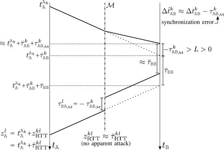
Figure 3: Illustration of an example attack against a PTP implementation that violates the second necessary condition.

The third condition is similar to the proposal in [11] of measuring the path delays during initialization and monitoring the delays during normal operation. However, [11] requires that B respond to A with zero delay during initialization to enable measurement of the reference delays. This condition is sufficient, but not necessary for secure synchronization. The system is in fact secure even if B is allowed a fixed layover time. Fig. 4 illustrates an example attack against a PTP implementation in violation of the third necessary condition. Note that the uncertainty of the a priori estimate of the RTT ($\bar{\sigma}_{\rm RTT}$) is larger than the alert limit, violating the third necessary condition which requires that the expected RTT be known to within the alert limit (and with much higher accuracy for provable sufficiency). Even though the measured RTT in this case is inconsistent with the expected RTT, it cannot be definitively flagged as an attack since benign variations in the RTT may also have led to the observed RTT.

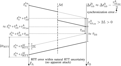
Figure 4: Illustration of an example attack against a PTP implementation that violates the third necessary condition.

Interestingly, at first sight, the third security condition in this paper does not resemble the proposed defense in [18] that enforces an upper bound on the synchronization error accumulated between sync messages and recommends that B send its timestamps to A periodically for verification. As explained next, this condition is in fact equivalent to the condition of known and measurable RTT, when adapted according to the system model considered in [18].

Note that the requirement of a zero delay in [11], or a short layover time in this paper, enables A to measure the RTT since the transmit time of the $l$th feature in $s_{\texttt{B}}$, that is $t_{\texttt{B}}^{\texttt{B}_{l}}$, can be approximately traced back to A’s clock to within the alert limit as $t_{\texttt{A}}^{\texttt{A}_{k}}+\bar{\tau}_{\texttt{AB}}^{k}+\bar{\tau}_{\texttt{BB}}$. Enforcing the synchronization error to within $L$ and transmitting B’s timestamp to A achieves the same objective for the defense in [18], since the transmit time from B can be traced back to A’s clock with the assumed approximate synchronization. Therefore, the proposed countermeasures in [11] and [18] are two different incarnations of the third security condition proposed in this paper. Of course, the failure of both [11] and [18] to address the second necessary condition makes their proposed defenses vulnerable to an adversary that can communicate along a shorter time path between A and B.

VI-B Alternative Compliant System

This section describes an alternative wireless clock synchronization protocol that satisfies the set of necessary and sufficient conditions presented in Section IV. The proposed protocol involves bi-directional exchange of GNSS-like pseudo-random codes for continuous clock synchronization, in contrast to discrete packet-based synchronization techniques such as NTP and PTP. It is offered here to illustrate the general applicability of the proposed necessary and sufficient conditions to a range of underlying protocols. Such a protocol can potentially be applied in two-way satellite time transfer and terrestrial wireless clock synchronization systems for continuous clock synchronization, in contrast to the packet-based discrete synchronization in NTP/PTP.

The time master A and the time seeker B communicate wirelessly over the LOS channel between the nodes. To simplify the analysis, it is assumed that A and B securely share long sequences of pseudo-random bits prior to synchronization. These sequences of bits will later enable generation of unpredictable signals. The pseudo-random sequence for A has the form

$$\bm{b}_{\texttt{A}}=\left\{b_{\texttt{A}}^{k}\right\}_{k=0}^{N},\quad b_{\texttt{A}}^{k}\in\left\{0,1\right\}$$

The pseudo-random code $C_{\texttt{A}}(t_{\texttt{A}})$ for A is then generated as

$$C_{\texttt{A}}(t_{\texttt{A}})=2b_{\texttt{A}}^{k}-1\text{ for }t_{\texttt{A}}\in[t_{\texttt{A}}^{\texttt{A}_{k}},t_{\texttt{A}}^{\texttt{A}_{k+1}}),k\in\{0,1,2,\dots\}$$

where $t_{\texttt{A}}^{\texttt{A}_{k}}$ denotes the time according to A at which the start of the $k$th bit in A’s signal is transmitted. The pseudo-random nature of $\bm{b}_{\texttt{A}}$ ensures that $C_{\texttt{A}}(t_{\texttt{A}})$ has good cross-correlation properties, which enables an accurate measurement of the time-of-arrival of A’s signal at B, that is, $\sigma_{\epsilon}\ll L$. Station A modulates a carrier with the code $C_{\texttt{A}}$ and transmits a signal $s_{\texttt{A}}(t_{\texttt{A}})$ whose complex baseband representation is given as

$$s_{\texttt{A}}(t_{\texttt{A}})=C_{\texttt{A}}(t_{\texttt{A}})\exp{\left(j\theta_{\texttt{A}}(t_{\texttt{A}})\right)}$$

This signal is received at B as

$$r_{\texttt{B}}(t_{\texttt{A}},\tau_{\texttt{AB}}) =s_{\texttt{A}}(t_{\texttt{A}}-\tau_{\texttt{AB}})+w_{\texttt{AB}}(t_{\texttt{A}})$$

$$=C_{\texttt{A}}(t_{\texttt{A}}-\tau_{\texttt{AB}})\exp{\left(j\theta_{\texttt{A}}(t_{\texttt{A}}-\tau_{\texttt{AB}})\right)}+w_{\texttt{AB}}(t_{\texttt{A}})$$

where all symbols have their usual meanings as detailed in Section III. Station B captures a window $R_{\texttt{B}}^{k}$ of $r_{\texttt{B}}$ and correlates it with a local replica of $C_{\texttt{A}}$. The result of the correlation enables B to detect the start of the $k$th bit of $C_{\texttt{A}}$ in the window, and provides a measurement

$$z_{\texttt{B}}^{k} =t_{\texttt{B}}^{\texttt{A}_{k}}+w_{\texttt{AB}}^{k}$$

of the time-of-arrival of the $k$th bit at B. Furthermore, the relationship between the start of the $k$th bit and $t_{\texttt{A}}^{\texttt{A}_{k}}$ enables B to infer the latter.

If a prior estimate $\bar{\tau}_{\texttt{AB}}^{k}$ of $\tau_{\texttt{AB}}^{k}$ is available, then B estimates the clock offset $\Delta t_{\texttt{AB}}^{k}$ as in (4).

Similar to the pseudo-random sequence and code construction for A, B generates its unpredictable code $C_{\texttt{B}}(t_{\texttt{B}})$. A and B agree on a one-to-one mapping between $C_{\texttt{A}}$ and $C_{\texttt{B}}$ such that B responds with the $l$th bit of $C_{\texttt{B}}$ on reception of the start of the $k$th bit of $C_{\texttt{A}}$. Furthermore, A and B agree that the start of the $l$th bit of $C_{\texttt{B}}$ will have a code-phase offset of $\bar{\tau}_{\texttt{BB}}$ with respect to the start of the $k$th bit of $C_{\texttt{A}}$. Station B transmits the response signal as

$$s_{\texttt{B}}(t_{\texttt{B}}) =C_{\texttt{B}}(t_{\texttt{B}})\exp{\left(j\theta_{\texttt{B}}(t_{\texttt{B}})\right)}$$

such that

$$t_{\texttt{B}}^{\texttt{B}_{l}} =z_{\texttt{B}}^{k}+\bar{\tau}_{\texttt{BB}}$$

according to the time at B. In true time, the epoch $t_{\texttt{B}}^{\texttt{B}_{l}}$ corresponds to

$$t_{\texttt{B}}^{\texttt{B}_{l}}\rightleftharpoons t_{\texttt{A}}^{\texttt{A}_{k}}+\tau_{\texttt{AB}}^{k}+w_{\texttt{AB}}^{k}+\tau_{\texttt{BB}}$$

Station A receives the response as

$$r_{\texttt{A}} =s_{\texttt{B}}(t_{\texttt{B}}-\tau_{\texttt{BA}})+w_{\texttt{BA}}(t_{\texttt{A}})$$

and captures a window of the signal $R_{\texttt{A}}^{l}$. A correlates $R_{\texttt{A}}^{l}$ with a local replica of $C_{\texttt{B}}$ to detect the start of the $l$th bit of $C_{\texttt{B}}$. This enables A to measure the time-of-arrival

$$z_{\texttt{A}}^{l} =t_{\texttt{A}}^{\texttt{B}_{l}}+w_{\texttt{BA}}^{l}$$

Moreover, the detection of the $l$th bit indicates that it was transmitted in response to the receipt of the start of the $k$th bit of $C_{\texttt{A}}$. Since A knows the start time of the $k$th bit as $t_{\texttt{A}}^{\texttt{A}_{k}}$, it measures the RTT as described in (6).

Note that the exchange of one-time pad sequences enables the proposed system to satisfy the first security condition. Wireless LOS communication satisfies the second security condition, and the knowledge of the code-phase layover offset enables A to make an accurate prior estimate of the RTT within the alert limit, thereby satisfying the third security condition. Thus, the proposed system complies with all three necessary and sufficient conditions for secure clock synchronization.

VII System Simulation

This section presents a simulation study of a secure clock synchronization model operating over a simplistic channel model. Unlike the abstract treatment of delays in the security derivations presented earlier, the simulation is carried out with models of delays experienced by the synchronization messages over a real channel. This study also expounds the interplay between slave clock stability, security requirements, attack models, and attack detection thresholds that must be determined in a practical synchronization system. The channel and attack models developed in this simulation are not comprehensive. Rather, relatively simple models are considered to clearly demonstrate the underlying principles. More sophisticated channel and attack models can similarly be analyzed by following the outline of this simulation.

VII-A Channel Model

The simulated system resembles a traditional local area network, and is schematically depicted in Fig. 5. As before, A and B are the time master and seeker stations, respectively. The messages between these stations pass through a series of $N$ routers. Each router is under network traffic loading generated by the nodes labeled T. The routers perform simple packet forwarding, i.e., no cryptographic operations or complex payload modifications are performed. Each router transmits the queued packets at a service rate of 1 Gbps. Each network packet is assumed to have a size of 1542 bytes. The MITM adversary $\mathcal{M}$ maliciously inserts itself along the communication path between A and B.

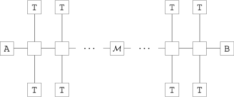
Figure 5: Schematic diagram of the network topology considered in this section.

The sync and response packets from A and B experience processing and queueing delay at each router, and propagation/link delay between routers. Queueing delay is the duration for which the packet is buffered in the router before it can be transmitted. Processing delay is the time taken by the router to process the packet header, for example, to determine the packet’s destination. Since the routers in this simulation perform simple packet forwarding, the processing delay is negligible as compared to the queueing delay [33]. The propagation/link delay is also insignificant for local networks because the propagation speed is a comparable fraction of the speed of light. Thus, only the queueing delay significantly contributes to the overall channel delay variations.

Let the network idle probability for a particular router, denoted by $\rho$, be defined as the probability of the router queue being empty at a randomly chosen time instant. Since the synchronization packets are delay-sensitive, the routers in this simulation implement non-preemptive priority scheduling for synchronization packets when the queue is not empty. This means that on arrival of a sync or response packet, the router is allowed to complete the transmission of the data packet currently being serviced, if any, but is required to service the delay-sensitive packet before the other network data in the queue. Since the time period between consecutive sync-response pairs is quite large as compared to the RTT for a given pair, it is assumed that a router never has more than one delay-sensitive packet in its queue. Under such scheduling, the delay experienced by the timing messages is best modeled as follows: with probability $\rho$, the total router delay is zero, and with probability ($1-\rho$) the total router delay is uniformly distributed between zero and the maximum time to service a packet of length 1542 bytes ($1542\times 8\times 2^{-30}\approx 11.49$ microseconds for a Gigabit router).

Given the above channel specifications and values for $N$ and $\rho$, it is possible to perform a Monte Carlo simulation to obtain the anticipated RTT $\bar{\tau}_{\rm RTT}$, which is taken to be the empirical mean of the RTT measurements in the simulation, and the associated standard deviation $\bar{\sigma}_{\rm RTT}$. As shown in Fig. 6, in case of a single sync-response pair measurement, the RTT has an empirical mean of $80.34$ microseconds and an empirical standard deviation of $17.09$ microseconds with $N=10$ and $\rho=0.3$. Observe that even for a relatively small $N$, the empirical distribution approaches the Gaussian shape, but has slightly heavier tail on the higher end of the delay. The distribution for mean of batches of $10$ observations has a smaller empirical standard deviation of $5.41$ microseconds.

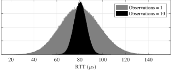
Figure 6: Empirical distribution of the RTT of sync-response pairs through a network of $N=10$ routers with network idle probability of $\rho=0.3$. The light-shaded histogram shows the empirical distribution of the RTT of a single sync-response pair. The dark-shaded histogram shows the corresponding distribution for the mean of batches of $10$ observations of the RTT.

VII-B System and Security Requirements

The clock at the time seeker B drifts with respect to the true time clock at A unless corrected by a sync message from A. As before, let $L$ denote the alert limit for the system. Let $T$ denote a time duration over which a perfectly synchronized clock at B at the beginning of the duration, absent an adversary, drifts more than $L_{\mathcal{N}}$ for some $L_{\mathcal{N}}<L$ with a probability smaller than an acceptably small bound $\mathbb{P}_{\epsilon}$.

In the system under simulation, the clock offset for B is estimated and corrected for every $T$ seconds. By definition of $T$, it holds that if the clocks at A and B are perfectly synchronized after every $T$ seconds, then the natural drift envelope of B’s clock does not exceed $L$ with an unacceptably high probability. Define

$$L_{\mathcal{M}}\triangleq L-L_{\mathcal{N}}$$

Observe that if an adversary is able to introduce a synchronization error larger than $L_{\mathcal{M}}$, then the system is compromised since the natural drift of the clock at B could potentially lead to a clock offset greater than $L$ before the next synchronization interval, with a probability greater than $\mathbb{P}_{\epsilon}$. Thus, A must flag any adversarial delay greater than $L-L_{\mathcal{N}}$ with probability higher than a desired detection probability, denoted by $\mathbb{P}_{\rm D}$. It is worth noting that this practical complication of the magnitude of $L_{\mathcal{N}}$ was abstracted in the sufficiency proof, where the threshold was set to $L-\delta$ for $\delta>0$.

In general, A makes multiple measurements of the RTT between A and B over the time period $T$. As shown in Fig. 6, the mean of multiple observations over $T$ has a distribution with a smaller standard deviation as compared to that of a single observation. In the simulated system, if no attack is detected, A updates $\bar{\tau}_{\texttt{AB}}^{k}$ every $T$ seconds based on the empirical mean of the RTT measurements made over that period. Note that even though $\bar{\tau}_{\texttt{AB}}^{k}$ is updated based on the measurements, no updates are applied to $\bar{\tau}_{\rm RTT}$ and $\bar{\sigma}_{\rm RTT}$, which are predetermined by simulation or measurements under a secure calibration campaign.

The empirical mean of the measured RTT is taken as the test statistic to detect an attack. For the attack model detailed next, it can be shown that this test statistic becomes optimal for large values of $N$ [34].

VII-C Attack Model

The synchronization system considered in this simulation complies with the necessary security conditions presented in this paper. Consequently, the adversary $\mathcal{M}$ is unable to advance the sync or response messages, and can only increase the RTT measured by A relative to the authentic RTT. This simulation considers a simple adversary model that introduces a fixed delay in the measured RTT. In order to conceal its presence while compromising synchronization with appreciable probability, $\mathcal{M}$ introduces a delay of $L_{\mathcal{M}}+\xi$ seconds for some small $\xi>0$.

Let $H_{0}$ denote the null hypothesis (no attack), and $H_{1}$ denote the alternative hypothesis. Under $H_{0}$, the measured RTT at A is drawn from the distribution that was used to calibrate/simulate the channel delay distribution, while under $H_{1}$, the measured RTT is drawn from a distribution that is shifted from the calibration distribution by $L_{\mathcal{M}}+\xi$. This is visually depicted in Fig. 7. Given a detection threshold $\lambda$, the dark-shaded region in Fig. 7 denotes the probability of false alarm, $\mathbb{P}_{\rm F}$, while the light-shaded region denotes the probability of missed detection ($1-\mathbb{P}_{\rm D}$). In observing Fig. 7, it might be argued, and holds true, that a reasonable attacker may introduce noise in the introduced delay to inflate the width of the distribution under $H_{1}$ and thereby decrease the probability of detection of an attack. However, in that case, the empirical mean test statistic is no longer optimal. Instead, A would incorporate the observed variance of the RTT in its test statistic in addition to the empirical mean. In short, the attack model in this simulation is not comprehensive, as explained previously. For a more sophisticated treatment of sensor deception and protection techniques, the reader may refer to [35].

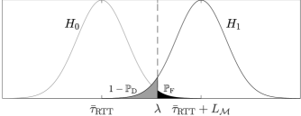
Figure 7: Representation of the distributions under $H_{0}$ and $H_{1}$ along with the detection threshold and the associated $\mathbb{P}_{\rm F}$ and $\mathbb{P}_{\rm D}$.

VII-D Simulation

The system and attack described above have been simulated with $N=10$ and $\rho=0.3$ for all routers. The adversarial delay $L_{\mathcal{M}}+\xi$ is set to 10 microseconds, and the required probability of detection $\mathbb{P}_{\rm D}$ is set to $0.999$. The number of RTT observations made in time $T$ are varied between $1$ and $200$. Given the number of observations, and a required $\mathbb{P}_{\rm D}$, the system is simulated under $H_{1}$ for $10^{6}$ detection epochs and the maximum possible detection threshold $\lambda$ that satisfies the detection probability is obtained. Subsequently, the system is simulated under $H_{0}$ and the number of test statistics exceeding the threshold $\lambda$ are recorded. The frequency of such epochs is reported as the probability of false alarm $\mathbb{P}_{\rm F}$.

Fig. 8 shows the above procedure for $80$ RTT measurements made per test statistic. In this case, $\lambda$ is obtained to be 84.53 microseconds and the corresponding $\mathbb{P}_{\rm F}$ is $1.59\%$. Fig. 9 shows a log-log plot of $\mathbb{P}_{\rm F}$ as a function of the number of observations made per test statistic. When the number of observations is greater than $160$, no false alarms were observed with $10^{6}$ trials. For the given channel delay variation statistics, the probability of false alarm is very high for small number of observations per decision epoch since the threshold $\lambda$ that must be set to detect an attack with the required $\mathbb{P}_{\rm D}$ is large in comparison to the minimal delay that the adversary must introduce to compromise synchronization ($L_{\mathcal{M}}$). For a more stable channel, such as a wireless or PTP-aware channel, fewer measurements per decision epoch would suffice.

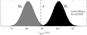
Figure 8: Distribution of the test statistic under $H_{0}$ and $H_{1}$ for $80$ RTT measurements per decision epoch. ($N=10$, $\rho=0.3$, $L_{\mathcal{M}}+\xi=10\mu$s, $\mathbb{P}_{\rm D}=0.999$)

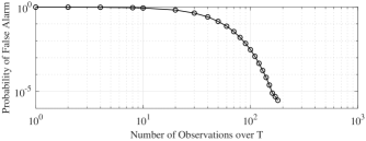
Figure 9: Probability of false alarm as a function of number of observations per decision epoch. ($N=10$, $\rho=0.3$, $L_{\mathcal{M}}+\xi=10\mu$s, $\mathbb{P}_{\rm D}=0.999$)

VII-E Practical Implications

Section V-A makes fairly remarkable assumptions about the synchronization system to show provably secure time transfer. For instance, it requires that errors in the a priori estimate of the RTT of the timing messages be negligible compared to the alert limit. Nonetheless, as shown in this section, for a given channel with bounded delay variations and a given slave clock, some level of security guarantee can be made for a synchronization system that satisfies the necessary and sufficient conditions presented herein. For concreteness, consider a system that requires an alert limit of $L=100$ microseconds and a slave clock that drifts no more than $L_{\mathcal{N}}=50$ microseconds over a period of $T=1$ second with acceptably high probability ($1-\mathbb{P}_{\epsilon}$). Then, for $N=10$ and $\rho=0.3$, if A makes 10 RTT measurements over 1 second, the empirical mean test statistic is distributed as the dark-shaded distribution in Fig. 6 with a standard deviation of $\approx 5.4$ microseconds. For $L_{\mathcal{M}}=L-L_{\mathcal{N}}=50$ microseconds, a threshold of $\approx\bar{\tau}_{\rm RTT}+30$ microseconds will yield a missed detection rate of approximately $1$ in $15000$, and a false alarm rate of approximately $3.5$ in $1$ million. With a more stable slave clock or more measurements per second, these probabilities can be made more favorable.

Another important concern that has not been addressed in the simulation is that of the incorporation of cryptographic constructs in the synchronization protocol. The encryption and decryption algorithms are often complex and take non-negligible processing time to execute. However, note that at A, the sync message is timestamped after the encryption process, and thus the time taken for encryption is inconsequential. At B, it is important to concede that the decryption of the sync message and the encryption of the response message cannot be assumed to happen instantaneously. This has been accounted for by allowing the layover time $\bar{\tau}_{\texttt{BB}}$ for the cryptographic processes to execute. Once again, the receipt timestamp of the response message at A is applied before the decryption process, and hence the decryption time at A is inconsequential. Thus, compliance with the first security condition must not pose significant practical challenges.

VIII Conclusions

A fundamental theory of secure clock synchronization was developed for a generic system model. The problem of secure clock synchronization was formalized with explicit assumptions, models, and definitions. It was shown that all possible one-way clock synchronization protocols are vulnerable to replay attacks. A set of necessary conditions for secure two-way clock synchronization was proposed and proved. Compliance with these necessary conditions with strict upper bounds was shown to be sufficient for secure clock synchronization, which is a significant result for provable security in critical infrastructure. The general applicability of the set of security conditions was demonstrated by specializing these conditions to design a secure PTP protocol and an alternative secure two-way clock synchronization protocol with GNSS-like signals. Results from a simulation with models of channel delays were presented to expound the interplay between slave clock stability, security requirements, attack models, and attack detection thresholds.

Lakshay Narula received the B.Tech. degree in electronics engineering from IIT-BHU, India, in 2014, and the M.S. degree in electrical and computer engineering from The University of Texas at Austin, Austin, TX, USA, in 2016. He is currently a Ph.D. student with the Department of Electrical and Computer Engineering at The University of Texas at Austin, and a Graduate Research Assistant at the UT Radionavigation Lab. His research interests include GNSS signal processing, secure perception in autonomous systems, and detection and estimation. Lakshay has previously been a visiting student at the PLAN Group at University of Calgary, Calgary, AB, Canada, and a systems engineer at Accord Software & Systems, Bangalore, India. He was a recipient of the 2017 Qualcomm Innovation Fellowship.

Todd E. Humphreys received the B.S. and M.S. degrees in electrical and computer engineering from Utah State University, Logan, UT, USA, in 2000 and 2003, respectively, and the Ph.D. degree in aerospace engineering from Cornell University, Ithaca, NY, USA, in 2008. He is an Associate Professor with the Department of Aerospace Engineering and Engineering Mechanics, The University of Texas (UT) at Austin, Austin, TX, USA, and Director of the UT Radionavigation Laboratory. He specializes in the application of optimal detection and estimation techniques to problems in satellite navigation, autonomous systems, and signal processing. His recent focus has been on secure perception for autonomous systems, including navigation, timing, and collision avoidance, and on centimeter-accurate location for the mass market. Dr. Humphreys received the University of Texas Regents’ Outstanding Teaching Award in 2012, the National Science Foundation CAREER Award in 2015, and the Institute of Navigation Thurlow Award in 2015.

References

- [1] A. Phadke, B. Pickett, M. Adamiak, M. Begovic, G. Benmouyal, R. Burnett Jr, T. Cease, J. Goossens, D. Hansen, M. Kezunovic et al., “Synchronized sampling and phasor measurements for relaying and control,” IEEE Transactions on Power Delivery, vol. 9, no. 1, pp. 442–452, 1994.
- [2] J. G. McNeff, “The global positioning system,” IEEE Transactions on Microwave Theory and Techniques, vol. 50, no. 3, pp. 645–652, 2002.
- [3] J. J. Angel, “When finance meets physics: The impact of the speed of light on financial markets and their regulation,” Financial Review, vol. 2, no. 49, pp. 271–281, 2014.
- [4] J. C. Corbett, J. Dean, M. Epstein, A. Fikes, C. Frost, J. J. Furman, S. Ghemawat, A. Gubarev, C. Heiser, P. Hochschild et al., “Spanner: Google’s globally distributed database,” ACM Transactions on Computer Systems (TOCS), vol. 31, no. 3, p. 8, 2013.
- [5] L. D. Shapiro, “Time synchronization from Loran-C,” IEEE Spectrum, vol. 8, no. 5, pp. 46–55, 1968.
- [6] A. Bauch, P. Hetzel, and D. Piester, “Time and frequency dissemination with DCF77: From 1959 to 2009 and beyond,” PTB-Mitteilungen, vol. 119, no. 3, pp. 3–26, 2009.
- [7] D. W. Allan and M. A. Weiss, Accurate time and frequency transfer during common-view of a GPS satellite. Electronic Industries Association, 1980.
- [8] M. L. Psiaki and T. E. Humphreys, “GNSS spoofing and detection,” Proceedings of the IEEE, vol. 104, no. 6, pp. 1258–1270, 2016.
- [9] K. D. Wesson, J. N. Gross, T. E. Humphreys, and B. L. Evans, “GNSS signal authentication via power and distortion monitoring,” IEEE Transactions on Aerospace and Electronic Systems, 2018, to be published; preprint available at https://arxiv.org/abs/1702.06554.
- [10] D. Chou, L. Heng, and G. Gao, “Robust GPS-based timing for phasor measurement units: A position-information-aided approach,” in Proceedings of the ION GNSS+ Meeting, 2014.
- [11] M. Ullmann and M. Vögeler, “Delay attacks — Implication on NTP and PTP time synchronization,” in Precision Clock Synchronization for Measurement, Control and Communication, 2009. ISPCS 2009. International Symposium on. IEEE, 2009, pp. 1–6.
- [12] T. Mizrahi, “A game theoretic analysis of delay attacks against time synchronization protocols,” in Precision Clock Synchronization for Measurement Control and Communication (ISPCS), 2012 International IEEE Symposium on. IEEE, 2012, pp. 1–6.
- [13] B. Moussa, M. Debbabi, and C. Assi, “A detection and mitigation model for PTP delay attack in an IEC 61850 substation,” IEEE Transactions on Smart Grid, 2016.
- [14] Q. Yang, D. An, and W. Yu, “On time desynchronization attack against IEEE 1588 protocol in power grid systems,” in Energytech, 2013 IEEE. IEEE, 2013, pp. 1–5.
- [15] J.-C. Tournier and O. Goerlitz, “Strategies to secure the IEEE 1588 protocol in digital substation automation,” in Critical Infrastructures, 2009. CRIS 2009. Fourth International Conference on. IEEE, 2009, pp. 1–8.
- [16] S. Bhamidipati, Y. Ng, and G. X. Gao, “Multi-receiver GPS-based direct time estimation for PMUs,” in Proceedings of the 29th International Technical Meeting of The Satellite Division of the Institute of Navigation (ION GNSS+ 2016), Portland, OR, 2016.
- [17] Y. Ng and G. X. Gao, “Robust GPS-based direct time estimation for PMUs,” in Position, Location and Navigation Symposium (PLANS), 2016 IEEE/ION. IEEE, 2016, pp. 472–476.
- [18] R. Annessi, J. Fabini, and T. Zseby, “SecureTime: Secure multicast time synchronization,” arXiv preprint arXiv:1705.10669, 2017.
- [19] L. Narula and T. E. Humphreys, “Requirements for secure wireless time transfer,” in Proceedings of the IEEE/ION PLANS Meeting, Savannah, GA, 2016.
- [20] R. C. Merkle, “Secure communications over insecure channels,” Communications of the ACM, vol. 21, no. 4, pp. 294–299, 1978.
- [21] C. H. Bennett and G. Brassard, “Quantum cryptography: Public key distribution and coin tossing,” 1984.
- [22] A. K. Ekert, “Quantum cryptography based on Bell’s theorem,” Physical review letters, vol. 67, no. 6, p. 661, 1991.
- [23] P. Misra and P. Enge, Global Positioning System: Signals, Measurements, and Performance, revised second ed. Lincoln, Massachusetts: Ganga-Jumana Press, 2012.
- [24] K. D. Wesson, M. P. Rothlisberger, and T. E. Humphreys, “A proposed navigation message authentication implementation for civil GPS anti-spoofing,” in Proceedings of the ION GNSS Meeting. Portland, Oregon: Institute of Navigation, 2011.
- [25] D. M. Akos, “Who’s afraid of the spoofer? GPS/GNSS spoofing detection via automatic gain control (AGC),” Navigation, Journal of the Institute of Navigation, vol. 59, no. 4, pp. 281–290, 2012.
- [26] T. E. Humphreys, Springer Handbook of Global Navigation Satellite Systems. Springer, 2017, ch. Interference, pp. 469–504.
- [27] M. Meurer, A. Konovaltsev, M. Cuntz, and C. Hättich, “Robust joint multi-antenna spoofing detection and attitude estimation using direction assisted multiple hypotheses RAIM,” in Proceedings of the 25th Meeting of the Satellite Division of the Institute of Navigation (ION GNSS+ 2012). ION, 2012.
- [28] D. Borio, “PANOVA tests and their application to GNSS spoofing detection,” IEEE Transactions on Aerospace and Electronic Systems, vol. 49, no. 1, pp. 381–394, Jan. 2013.
- [29] M. Bellare and C. Namprempre, “Authenticated encryption: Relations among notions and analysis of the generic composition paradigm,” Advances in Cryptology–ASIACRYPT 2000, pp. 531–545, 2000.
- [30] S. Goldwasser, S. Micali, and R. L. Rivest, “A digital signature scheme secure against adaptive chosen-message attacks,” SIAM Journal on Computing, vol. 17, no. 2, pp. 281–308, 1988.
- [31] A. Mahmood, G. Gaderer, H. Trsek, S. Schwalowsky, and N. Kerö, “Towards high accuracy in IEEE 802.11 based clock synchronization using PTP,” in Precision Clock Synchronization for Measurement Control and Communication (ISPCS), 2011 International IEEE Symposium on. IEEE, 2011, pp. 13–18.
- [32] T. Cooklev, J. C. Eidson, and A. Pakdaman, “An implementation of IEEE 1588 over IEEE 802.11b for synchronization of wireless local area network nodes,” IEEE Transactions on Instrumentation and Measurement, vol. 56, no. 5, pp. 1632–1639, Oct. 2007.
- [33] R. Ramaswamy, N. Weng, and T. Wolf, “Characterizing network processing delay,” in Global Telecommunications Conference, 2004. GLOBECOM’04. IEEE, vol. 3. IEEE, 2004, pp. 1629–1634.
- [34] H. L. Van Trees, Detection, estimation, and modulation theory, part I: detection, estimation, and linear modulation theory. John Wiley & Sons, 2004.
- [35] J. Bhatti and T. Humphreys, “Hostile control of ships via false GPS signals: Demonstration and detection,” Navigation, Journal of the Institute of Navigation, vol. 64, no. 1, 2017.