A successive difference-of-convex approximation method for a class of nonconvex nonsmooth optimization problems

Abstract

We consider a class of nonconvex nonsmooth optimization problems whose objective is the sum of a smooth function and a finite number of nonnegative proper closed possibly nonsmooth functions (whose proximal mappings are easy to compute), some of which are further composed with linear maps. This kind of problems arises naturally in various applications when different regularizers are introduced for inducing simultaneous structures in the solutions. Solving these problems, however, can be challenging because of the coupled nonsmooth functions: the corresponding proximal mapping can be hard to compute so that standard first-order methods such as the proximal gradient algorithm cannot be applied efficiently. In this paper, we propose a successive difference-of-convex approximation method for solving this kind of problems. In this algorithm, we approximate the nonsmooth functions by their Moreau envelopes in each iteration. Making use of the simple observation that Moreau envelopes of nonnegative proper closed functions are continuous difference-of-convex functions, we can then approximately minimize the approximation function by first-order methods with suitable majorization techniques. These first-order methods can be implemented efficiently thanks to the fact that the proximal mapping of each nonsmooth function is easy to compute. Under suitable assumptions, we prove that the sequence generated by our method is bounded and any accumulation point is a stationary point of the objective. We also discuss how our method can be applied to concrete applications such as nonconvex fused regularized optimization problems and simultaneously structured matrix optimization problems, and illustrate the performance numerically for these two specific applications.

1 Introduction

In this paper, we consider the following possibly nonconvex nonsmooth optimization problem:

$$\begin{array}[]{ll}\underset{\bm{x}}{\mbox{minimize}}&\displaystyle{F(\bm{x}):=f(\bm{x})+P_{0}(\bm{x})+\sum_{i=1}^{m}P_{i}(\mathcal{A}_{i}\bm{x}),}\end{array}$$ (1)

with the objective satisfying the following assumptions (see the next section for notation and definitions):

1. $f:\mathbb{R}^{n}\rightarrow\mathbb{R}$ is an $L$-smooth function i.e., there exists a constant $L>0$ so that

   $$\|\nabla f(\bm{x})-\nabla f(\bm{v})\|\leq L\|\bm{x}-\bm{v}\|$$

   for any $\bm{x}$, $\bm{v}\in\mathbb{R}^{n}$.

2. $\mathcal{A}_{i}:\mathbb{R}^{n}\rightarrow\mathbb{R}^{n_{i}}$, $i=1,\ldots,m$, are linear mappings and $P_{i}:\mathbb{R}^{n_{i}}\rightarrow\mathbb{R}_{+}\cup\{\infty\}$, $i=0,\ldots,m$, are proper closed functions. The functions $P_{i}$, $i=0,\ldots,m$, are continuous in their respective domains, and

   $${\rm dom}\,P_{0}\cap\bigcap_{i=1}^{m}\mathcal{A}_{i}^{-1}({\rm dom}\,P_{i})\neq\emptyset.$$

   Moreover, the proximal mapping of $\gamma P_{i}$ is easy to compute for every $\gamma>0$ and for each $i=0,\ldots,m$. The sets ${\rm dom}\,P_{i}$, $i=1,\ldots,m$, are closed.

3. The function $f+P_{0}$ is level-bounded, i.e., for each $r\in\mathbb{R}$, the set $\{\bm{x}\in\mathbb{R}^{n}:f(\bm{x})+P_{0}(\bm{x})\leq r\}$ is bounded.

Problem (1) arises in many contemporary applications such as structured low rank matrix recovery problems (see, for example, Markovsky2008 ), nonconvex fused regularized optimization problems (see, for example, ParakhSelesnick15 and Example 2 in Section 4) and simultaneously structured matrix optimization problems (see, for example, Richard, et al. (2010) and Example 5 in Section 4). In these applications, the $P_{i}$’s are used for inducing desirable structures in the solutions and they are typically functions whose proximal mappings are easy to compute. If only one such function appears in (1), i.e., $m=0$, then some standard first-order methods such as the proximal gradient algorithm or its variants can be applied to solving (1) efficiently, because these algorithms only require the computation of $\nabla f$ and the proximal mapping of $\gamma P_{0}$ ($\gamma>0$) in each iteration. However, in all the aforementioned applications, there are always more than one such structure-inducing functions in (1) (i.e., $m\geq 1$) and the ${\cal A}_{i}$’s might not always be identity mappings. Then the proximal gradient algorithm and its variants cannot be applied efficiently, because the proximal mapping of $\bm{x}\mapsto P_{0}(\bm{x})+\sum_{i=1}^{m}P_{i}(\mathcal{A}_{i}\bm{x})$ can be hard to compute in general.

When the function $f$ and the $P_{i}$’s are all convex functions, one alternative approach for solving (1) is the alternating direction method of multipliers (ADMM); see, for example, EckBer92 ; GabMer76 . This method can be applied to (1) by suitably introducing slack variables that transform the problem into a linearly constrained problem, and each iteration only requires computing the proximal mappings of $f$ and $\gamma P_{i}$’s, as well as an update of an auxiliary (dual) variable. However, it is known that the ADMM does not necessarily converge if the $P_{i}$’s are nonconvex and $m\geq 1$; see, for example, (LiPong15, , Example 7). In the case when $P_{i}$’s are nonconvex but globally Lipschitz for $i=0,\ldots,m$ , and ${\cal A}_{i}$ is the identity mapping for all $i$, a new method for solving (1) was introduced in a series of work Yu2013 ; Yu2015 . Their method is based on the so-called proximal average of $P_{i}$’s, and each iteration involves only the computations of $\nabla f$ and the proximal mappings of $\gamma P_{i}$’s. However, it was only shown that any accumulation point of the sequence generated by their method is a stationary point of a certain smooth approximation of (1). Moreover, their method was designed for the case when $P_{i}$’s are globally Lipschitz, and the convergence behavior of their method is unknown when some non-Lipschitz functions such as the $\ell_{p}$ quasi-norm or the indicator function of some closed sets (such as the set of all $k$-sparse vectors) are present in (1).

In this paper, we propose a new method for solving (1) that is ready to take advantage of the ease of proximal mapping computations and has convergence guarantee under suitable assumptions, without imposing convexity nor globally Lipschitz continuity on $P_{i}$’s. We call our method the successive difference-of-convex approximation method (SDCAM). In this method, we construct an approximation to the objective of (1) in each iteration using the Moreau envelopes of the $\lambda_{i,t}P_{i}$, $i=1,\ldots,m$, where $t$ is the number of iteration and $\{\lambda_{i,t}\}$ are nonincreasing positive sequences satisfying $\lim_{t\to\infty}\lambda_{i,t}=0$; a suitable approximate stationary point of this approximation function is then taken to be the next iterate $\bm{x}^{t+1}$ of our algorithm. The point $\bm{x}^{t+1}$ can be found efficiently by recalling that the Moreau envelopes involved, despite being nonsmooth in general due to the possible nonconvexity of the $P_{i}$’s, are continuous difference-of-convex functions. Thus, one can incorporate majorization techniques in some standard first-order methods such as the proximal gradient algorithm for finding $\bm{x}^{t+1}$ in each iteration. Moreover, when such first-order methods are applied, the main computational cost per inner iteration typically only depends on the computations of $\nabla f$ and the proximal mappings of $\gamma P_{i}$, $i=0,\ldots,m$, $\gamma>0$, which are inexpensive in many applications. This suggests that the SDCAM can be applied efficiently for solving (1). More details of this algorithm will be discussed in Section 3, where we also prove that the sequence $\{\bm{x}^{t}\}$ generated is bounded and any accumulation point is a stationary point of (1) under suitable assumptions.

The rest of the paper is organized as follows. In Section 2, we introduce notation and some preliminary results. Our SDCAM is presented and its convergence is analyzed under suitable assumptions in Section 3. We then discuss how our method can be applied to various kinds of structured optimization problems including some nonconvex fused regularized optimization problems, some simultaneously sparse and low rank matrix optimization problems, and the low rank nearest correlation matrix problem, in Section 4. We also perform numerical experiments on some of these applications to demonstrate the efficiency of our algorithm in Section 5. Finally, we present some concluding remarks in Section 6.

2 Notation and preliminaries

In this paper, vectors and matrices are represented in bold lower case letters and upper case letters, respectively. The inner product of two vectors $\bm{a}$ and $\bm{b}\in\mathbb{R}^{n}$ are denoted by $\bm{a}^{\top}\bm{b}$ or $\bm{b}^{\top}\bm{a}$, and we use $\|\bm{a}\|_{0}$, $\|\bm{a}\|_{1}$ and $\|\bm{a}\|$ to denote the number of nonzero entries, the $\ell_{1}$ norm and the $\ell_{2}$ norm of $\bm{a}$, respectively. Moreover, we use $\mathrm{Diag}(\bm{a})$ to denote the diagonal matrix whose diagonal is $\bm{a}$. For two matrices $\bm{A}$ and $\bm{B}\in\mathbb{R}^{m{\times}n}$, their Hadamard (entrywise) product is denoted by $\bm{A}\circ\bm{B}$. We also use $\|\bm{A}\|_{*}$ and $\|\bm{A}\|_{F}$ to denote the nuclear norm and the Fröbenius norm of $\bm{A}$, respectively, and let ${\mbox{$\rm vec$}}(\bm{A})\in\mathbb{R}^{mn{\times}1}$ denote the vectorization of $\bm{A}$, which is obtained by stacking the columns of $\bm{A}$ on top of one another. Furthermore, we use $\sigma_{\max}(\bm{A})$ to denote the largest singular value of $\bm{A}$. The space of symmetric $n\times n$ matrices is denoted by $\mathcal{S}^{n}$. For a matrix $\bm{X}\in\mathcal{S}^{n}$, we use $\mathrm{diag}(\bm{X})\in\mathbb{R}^{n}$ to denote its diagonal and $\lambda_{\max}(\bm{X})$ to denote its largest eigenvalue. We write $\bm{X}\succeq 0$ if $\bm{X}$ is positive semidefinite. For a linear operator $\mathcal{A}$, we let $\mathcal{A}^{*}$ denote its adjoint.

A function $h:\mathbb{R}^{n}\to\mathbb{R}\cup\{\infty\}$ is said to be proper if ${\rm dom}\,h:=\{\bm{x}:\;h(\bm{x})<\infty\}\neq\emptyset$. Such a function is said to be closed if it is lower semicontinuous. Following (RockWets98, , Definition 8.3), for a proper function $h$, the limiting and horizon subdifferentials at $\bm{x}\in{\rm dom}\,h$ are defined respectively as

$$\begin{split}&\partial h(\bm{x})=\left\{\bm{u}:\;\exists\bm{u}^{t}\to\bm{u},\bm{x}^{t}\stackrel{{\scriptstyle h}}{{\to}}\bm{x}\ \ \mbox{with}\ \bm{u}^{t}\in\hat{\partial}h(\bm{x}^{t})\ \mbox{for each $t$}\right\},\\ &\partial^{\infty}h(\bm{x})=\left\{\bm{u}:\;\exists\alpha_{t}\downarrow 0,\alpha_{t}\bm{u}^{t}\to\bm{u},\bm{x}^{t}\stackrel{{\scriptstyle h}}{{\to}}\bm{x}\ \ \mbox{with}\ \bm{u}^{t}\in\hat{\partial}h(\bm{x}^{t})\ \mbox{for each $t$}\right\},\end{split}$$

where $\hat{\partial}h(\bm{w}):=\left\{\bm{u}:\;\liminf\limits_{\bm{y}\to\bm{w},\bm{y}\neq\bm{w}}\frac{h(\bm{y})-h(\bm{w})-{\bm{u}}^{\top}(\bm{y}-\bm{w})}{\|\bm{y}-\bm{w}\|}\geq 0\right\}$, and the notation $\bm{x}^{t}\stackrel{{\scriptstyle h}}{{\to}}\bm{x}$ means $\bm{x}^{t}\to\bm{x}$ and $h(\bm{x}^{t})\to h(\bm{x})$. We also define $\partial h(\bm{x})=\partial^{\infty}h(\bm{x}):=\emptyset$ when $\bm{x}\notin{\rm dom}\,h$. It is easy to show that at any $\bm{x}\in{\rm dom}\,h$, the limiting and horizon subdifferentials have the following robustness property:

$$\begin{split}\{\bm{u}:\;\exists\bm{u}^{t}\to\bm{u},\bm{x}^{t}\stackrel{{\scriptstyle h}}{{\to}}\bm{x}\ \mbox{with}\ \bm{u}^{t}\in\partial h(\bm{x}^{t})\ \mbox{for each }t\}&\subseteq\partial h(\bm{x}),\\ \{\bm{u}:\;\exists\alpha_{t}\downarrow 0,\alpha_{t}\bm{u}^{t}\to\bm{u},\bm{x}^{t}\stackrel{{\scriptstyle h}}{{\to}}\bm{x}\ \mbox{with}\ \bm{u}^{t}\in\partial h(\bm{x}^{t})\ \mbox{for each }t\}&\subseteq\partial^{\infty}h(\bm{x}).\end{split}$$ (2)

The limiting subdifferential at $\bm{x}$ reduces to $\{\nabla h(\bm{x})\}$ if $h$ is continuously differentiable at $\bm{x}$ (RockWets98, , Exercise 8.8(b)), and reduces to the convex subdifferential if $h$ is proper convex (RockWets98, , Proposition 8.12).

For a proper closed function $h$ with $\inf h>-\infty$, we will also need its Moreau envelope for any given $\lambda>0$, which is defined as

$$e_{\lambda}h(\bm{x}):=\inf_{\bm{y}}\left\{\frac{1}{2\lambda}\|\bm{x}-\bm{y}\|^{2}+h(\bm{y})\right\}.$$

This function is finite everywhere (RockWets98, , Theorem 1.25). It is not hard to see that

$$e_{\lambda}h(\bm{x})\leq h(\bm{x})$$ (3)

for all $\bm{x}$. The infimum in the definition of Moreau envelope is attained at the so-called proximal mapping of $\lambda h$ at $\bm{x}$, which is defined as

$${\mbox{\boldmath$\rm prox$}}_{\lambda h}(\bm{x}):=\operatornamewithlimits{Argmin}_{\bm{u}\in\mathbb{R}^{n}}\left\{\frac{1}{2\lambda}\|\bm{x}-\bm{u}\|^{2}+h(\bm{u})\right\}.$$

This set is always nonempty because $h$ is proper closed and bounded below (RockWets98, , Theorem 1.25). Let $\bm{\zeta}_{\lambda}\in{\mbox{\boldmath$\rm prox$}}_{\lambda h}(\bm{x})$. Then we have from (RockWets98, , Theorem 10.1) and (RockWets98, , Exercise 8.8(c)) that

$$\frac{1}{\lambda}(\bm{x}-\bm{\zeta}_{\lambda})\in\partial h(\bm{\zeta}_{\lambda}).$$ (4)

Furthermore, we have the following simple lemma, which should be well known. We provide a short proof for self-containedness.

Lemma 1

Let $h$ be a proper closed function with $\inf h>-\infty$ and let $\bm{x}^{*}\in{\rm dom}\,h$. Suppose that $\bm{x}^{t}\to\bm{x}^{*}$, $\lambda_{t}\downarrow 0$ and pick any $\bm{\zeta}^{t}\in{\mbox{\boldmath$\rm prox$}}_{\lambda_{t}h}(\bm{x}^{t})$ for each $t$. Then it holds that $\bm{\zeta}^{t}\in{\rm dom}\,h$ for all $t$ and $\bm{\zeta}^{t}\to\bm{x}^{*}$.

Proof

Under the assumptions, we have the following inequality:

$$\frac{1}{2\lambda_{t}}\|\bm{x}^{t}-\bm{\zeta}^{t}\|^{2}+\inf h\leq\frac{1}{2\lambda_{t}}\|\bm{x}^{t}-\bm{\zeta}^{t}\|^{2}+h(\bm{\zeta}^{t})=e_{\lambda_{t}}h(\bm{x}^{t})\leq\frac{1}{2\lambda_{t}}\|\bm{x}^{t}-\bm{x}^{*}\|^{2}+h(\bm{x}^{*}).$$

Hence, we have $\bm{\zeta}^{t}\in{\rm dom}\,h$ for all $t$ and

$$\|\bm{\zeta}^{t}-\bm{x}^{*}\|\leq\|\bm{\zeta}^{t}-\bm{x}^{t}\|+\|\bm{x}^{t}-\bm{x}^{*}\|\leq\sqrt{2\lambda_{t}(h(\bm{x}^{*})-\inf h)+\|\bm{x}^{t}-\bm{x}^{*}\|^{2}}+\|\bm{x}^{t}-\bm{x}^{*}\|\to 0.$$

$\Box$

Finally, recall that for a nonempty closed set $C$, the indicator function is defined as

$$\delta_{C}(\bm{x})=\begin{cases}0&{\rm if}\ \bm{x}\in C,\\ \infty&{\rm else}.\end{cases}$$

We define the (limiting) normal cone at any $\bm{x}\in C$ as $N_{C}(\bm{x}):=\partial\delta_{C}(\bm{x})$. We let ${\rm dist}(\bm{x},C):=\inf_{\bm{y}\in C}\|\bm{y}-\bm{x}\|$. The set of points in the nonempty closed set $C$ that are closest to a given $\bm{x}$ is denoted by ${\mbox{\boldmath$\rm proj$}}_{C}(\bm{x})$. One can observe that ${\mbox{\boldmath$\rm proj$}}_{C}={\mbox{\boldmath$\rm prox$}}_{\delta_{C}}$. The set ${\mbox{\boldmath$\rm proj$}}_{C}(\bm{x})$ at a given $\bm{x}$ is always nonempty for a nonempty closed set $C$, and is a singleton when $C$ is in addition convex.

3 Solution method for nonconvex nonsmooth optimization problems

3.1 Successive difference-of-convex approximation method

In this paper, we consider problem (1) and assume that its objective satisfies the assumptions A1, A2 and A3 in Section 1. We will discuss some concrete applications of (1) in more details in Section 4. In this section, we present an algorithm for solving (1).

Notice that (1) is in general a nonsmooth nonconvex optimization problem. The nonsmooth nonconvex function $P_{0}+\sum_{i=1}^{m}P_{i}\circ\mathcal{A}_{i}$ can be complicated in practice and handling it directly can be challenging. Indeed, although the proximal mappings of $\gamma P_{i}$, $i=0,\ldots,m$, are easy to compute, the proximal mapping of $P_{0}+\sum_{i=1}^{m}P_{i}\circ\mathcal{A}_{i}$ may be hard to evaluate and hence the classical proximal gradient algorithm and its variants cannot be adapted directly and efficiently for solving (1). In this paper, we suitably adapt a “smoothing” scheme for solving the above nonconvex nonsmooth problem. In this approach, in each iteration, we minimize the auxiliary function

$$F_{\bm{\lambda}}(\bm{x}):=f(\bm{x})+P_{0}(\bm{x})+\sum_{i=1}^{m}e_{\lambda_{i}}P_{i}(\mathcal{A}_{i}\bm{x})$$ (5)

approximately and then update $\bm{x}$ and ${\bm{\lambda}}=(\lambda_{1},\cdots,\lambda_{m})$, where $e_{\lambda_{i}}P_{i}$ is the Moreau envelope of $P_{i}$.

When $P_{i}$, $i=1,\ldots,m$ are all convex functions, the corresponding functions $e_{\lambda_{i}}P_{i}$ are Lipschitz differentiable (BauCom11, , Proposition 12.29). Hence, the function $F_{\bm{\lambda}}$ becomes the sum of a nonsmooth function $P_{0}$ and a smooth function, and can be minimized efficiently using, for example, the proximal gradient algorithm and its variants. This smoothing strategy has been widely used in the literature for convex problems; see Nes05 , and also BCG11 for a software package for convex optimization problems based on smoothing techniques. However, in our setting, $P_{i}$ is not necessarily convex. Thus, the corresponding Moreau envelope $e_{\lambda_{i}}P_{i}$ is not necessarily smooth and it is unclear whether $F_{\bm{\lambda}}$ can be minimized efficiently at first glance.

The key ingredient in our approach (where $P_{i}$ is possibly nonconvex) is the simple observation that for any nonnegative proper closed function $P$ and any $\mu>0$,

$$e_{\mu}P(\bm{u})=\frac{1}{2\mu}\|\bm{u}\|^{2}-\underbrace{\sup_{\bm{y}\in{\rm dom}\,P}\left\{\frac{1}{\mu}\bm{u}^{\top}\bm{y}-\frac{1}{2\mu}\|\bm{y}\|^{2}-P(\bm{y})\right\}}_{D_{\mu,P}(\bm{u})}.$$ (6)

Such a decomposition has been noted in Asplund73 when $P=\delta_{C}$ for some nonempty closed set $C$, and in (Lucet06, , Proposition 3) for the general case. Then $D_{\mu,P}$, as the supreme of affine functions and being finite-valued, is convex continuous. Moreover, using the definition of $e_{\mu}P(\bm{u})$, ${\mbox{\boldmath$\rm prox$}}_{\mu P}(\bm{u})$ and (6), we see that the supremum in $D_{\mu,P}(\bm{u})$ is attained at any point in ${\mbox{\boldmath$\rm prox$}}_{\mu P}(\bm{u})$. Let $\bm{y}^{*}\in{\mbox{\boldmath$\rm prox$}}_{\mu P}(\mathcal{A}\bm{x})$. Then $\bm{y}^{*}\in{\rm dom}\,P$ and we have for any $\bm{w}$ that

$$\begin{split}&D_{\mu,P}(\bm{w})-D_{\mu,P}({\cal A}\bm{x})\\ &=\sup_{\bm{y}\in{\rm dom}\,P}\left\{\frac{1}{\mu}\bm{w}^{\top}\bm{y}-\frac{1}{2\mu}\|\bm{y}\|^{2}-P(\bm{y})\right\}-\sup_{\bm{y}\in{\rm dom}\,P}\left\{\frac{1}{\mu}\bm{(}\mathcal{A}\bm{x})^{\top}\bm{y}-\frac{1}{2\mu}\|\bm{y}\|^{2}-P(\bm{y})\right\}\\ &\geq\frac{1}{\mu}\bm{w}^{\top}\bm{y}^{*}-\frac{1}{2\mu}\|\bm{y}^{*}\|^{2}-P(\bm{y}^{*})-\left(\frac{1}{\mu}\bm{(}\mathcal{A}\bm{x})^{\top}\bm{y}^{*}-\frac{1}{2\mu}\|\bm{y}^{*}\|^{2}-P(\bm{y}^{*})\right)\\ &=\frac{1}{\mu}{\bm{y}^{*}}^{\top}(\bm{w}-\mathcal{A}\bm{x}).\end{split}$$

This implies $\frac{1}{\mu}{\mbox{\boldmath$\rm prox$}}_{\mu P}(\mathcal{A}\bm{x})\subseteq\partial D_{\mu,P}(\mathcal{A}\bm{x})$, from which we deduce further that

$$\frac{1}{\mu}\mathcal{A}^{*}{\mbox{\boldmath$\rm prox$}}_{\mu P}(\mathcal{A}\bm{x})\subseteq\mathcal{A}^{*}\partial D_{\mu,P}(\mathcal{A}\bm{x})=\partial(D_{\mu,P}\circ\mathcal{A})(\bm{x}),$$ (7)

where the last equality follows from (Rock70, , Theorem 23.9) because $D_{\mu,P}$ is convex continuous. Thus, (5) is the sum of a smooth function $f$, a nonsmooth nonconvex function $P_{0}$ whose proximal mapping is easy to compute, and a continuous difference-of-convex function such that a subgradient corresponding to its concave part is easy to compute; thanks to (7) and Assumption A2. Proximal gradient methods with majorization techniques can then be suitably applied to minimizing (5). For instance, one can apply the NPG_major described in the appendix. Specifically, one can apply NPG_major with

$$h(\bm{x})=f(\bm{x})+\sum_{i=1}^{m}\frac{1}{2\lambda_{i}}\|\mathcal{A}_{i}\bm{x}\|^{2},\ P(\bm{x})=P_{0}(\bm{x}),\ g(\bm{x})=\sum_{i=1}^{m}D_{\lambda_{i},P_{i}}(\mathcal{A}_{i}\bm{x}).$$

It is routine to check that this choice of $h$, $P$ and $g$ satisfies the assumptions required in the appendix. Moreover, the $F_{\bm{\lambda}}$ is level-bounded because $f+P_{0}$ is level-bounded by assumption and $e_{\lambda_{i}}P_{i}$ are nonnegative for each $i=1,\ldots,m$ since $P_{i}$ are nonnegative. Finally, $F_{\bm{\lambda}}$ is continuous in its domain because $P_{0}$ is. Hence all assumptions required in the appendix for applying NPG_major are satisfied and the method can be applied to minimizing $F_{\bm{\lambda}}$ by initializing at any point $\bm{x}^{0}\in{\rm dom}\,P_{0}$.

We now describe our method for solving (1) with its update rules below in Algorithm 1. We call this method the successive difference-of-convex approximation method (SDCAM).

Algorithm 1 The SDCAM for (1)

Step 0.

Pick $m+1$ sequences of positive numbers with $\epsilon_{t}\downarrow 0$ and $\lambda_{i,t}\downarrow 0$ for $i=1,\ldots,m$, an $\bm{x}^{\rm feas}\in{\rm dom}\,P_{0}\cap\bigcap_{i=1}^{m}\mathcal{A}_{i}^{-1}({\rm dom}\,P_{i})$, and an $\bm{x}^{0}\in{\rm dom}\,P_{0}$. Set $t=0$.

Step 1.

If $F_{\bm{\lambda}_{t}}(\bm{x}^{t})\leq F_{\bm{\lambda}_{t}}(\bm{x}^{\rm feas})$, set $\bm{x}^{t,0}=\bm{x}^{t}$. Else, set $\bm{x}^{t,0}=\bm{x}^{\rm feas}$.

Step 2.

Approximately minimize $F_{\bm{\lambda}_{t}}(\bm{x})$, starting at $\bm{x}^{t,0}$, and terminating at $\bm{x}^{t,l_{t}}$ when

$$\begin{split}&{\rm dist}\left(0,\nabla f(\bm{x}^{t,l_{t}})+\partial P_{0}(\bm{x}^{t,l_{t}+1})+\sum_{i=1}^{m}\frac{1}{\lambda_{i,t}}\mathcal{A}^{*}_{i}[\mathcal{A}_{i}\bm{x}^{t,l_{t}}-{\mbox{\boldmath$\rm prox$}}_{\lambda_{i,t}P_{i}}(\mathcal{A}_{i}\bm{x}^{t,l_{t}})]\right)\leq\epsilon_{t},\\ &{\rm and}\ \ \ \ \|\bm{x}^{t,l_{t}+1}-\bm{x}^{t,l_{t}}\|\leq\epsilon_{t},\ \ \ \ F_{\bm{\lambda}_{t}}(\bm{x}^{t,l_{t}})\leq F_{\bm{\lambda}_{t}}(\bm{x}^{t,0}).\end{split}$$ (8)

Step 3.

Update $\bm{x}^{t+1}=\bm{x}^{t,l_{t}}$ and $t=t+1$. Go to Step 1.

We would like to point out that Step 1 in SDCAM is crucial in our convergence analysis: this strategy was also used in the penalty decomposition method in LuZh13 . As we shall see in the proof of Theorem 2 below, it ensures that (2) can be applied at an accumulation point of $\{\bm{x}^{t}\}$.

3.2 Theoretical guarantee for global convergence

In this section, we first discuss how $F_{\bm{\lambda}_{t}}$ can be approximately minimized so that (8) is satisfied at the $t$-th iteration and comment on the computational complexity. Then we prove the convergence of the SDCAM under suitable assumptions.

As discussed above, $F_{\bm{\lambda}_{t}}$ can be minimized by the NPG_major outlined in the appendix. Moreover, due to (7), one can choose $\bm{\zeta}^{t,l}=\sum_{i=1}^{m}\frac{1}{\lambda_{i,t}}\mathcal{A}_{i}^{*}\bm{\zeta}_{i}^{t,l}$ in the algorithm with

$$\bm{\zeta}_{i}^{t,l}\in{\mbox{\boldmath$\rm prox$}}_{\lambda_{i,t}P_{i}}(\mathcal{A}_{i}\bm{x}^{t,l})$$ (9)

for each $i=1,\ldots,m$ and $l\geq 0$ so that $\sum_{i=1}^{m}\frac{1}{\lambda_{i,t}}\mathcal{A}_{i}^{*}\bm{\zeta}_{i}^{t,l}$ lies in the subdifferential of $\sum_{i=1}^{m}(D_{\lambda_{i,t},P_{i}}\circ\mathcal{A}_{i})$ at $\bm{x}^{t,l}$. Using this special version of NPG_major, we can show that the termination criterion (8) is satisfied after finitely many inner iterations.

Theorem 1

Suppose that the NPG_major is applied with $\bm{\zeta}^{t,l}=\sum_{i=1}^{m}\frac{1}{\lambda_{i,t}}\mathcal{A}_{i}^{*}\bm{\zeta}_{i}^{t,l}$, where $\bm{\zeta}_{i}^{t,l}$ are chosen as in (9), to minimizing $F_{\bm{\lambda}_{t}}$ in the $t$-th iteration of SDCAM. Then the criterion (8) is satisfied after finitely many inner iterations.

Proof

According to the convergence properties of the NPG_major, one obtains a sequence $\{\bm{x}^{t,l}\}_{l\geq 0}$ satisfying

1. $\lim\limits_{l\to\infty}\|\bm{x}^{t,l+1}-\bm{x}^{t,l}\|=0$ (Proposition 2 in the appendix), $F_{\bm{\lambda}_{t}}(\bm{x}^{t,l})\leq F_{\bm{\lambda}_{t}}(\bm{x}^{t,0})$ (thanks to (68)); and

2. for any $l\geq 0$ (see (67)),

   $$\bm{x}^{t,l+1}\!\in\!\operatornamewithlimits{Argmin}_{\bm{x}}\left\{\left(\nabla f(\bm{x}^{t,l})+\sum_{i=1}^{m}\frac{\bm{\omega}^{t,l}_{i}}{\lambda_{i,t}}\right)^{\top}\!\!\bm{x}+\frac{\bar{L}_{t,l}}{2}\|\bm{x}-\bm{x}^{t,l}\|^{2}+P_{0}(\bm{x})\right\},$$ (10)

   where $\bm{\omega}^{t,l}_{i}:=\mathcal{A}_{i}^{*}[\mathcal{A}_{i}\bm{x}^{t,l}-\bm{\zeta}_{i}^{t,l}]$. Here, the sequence $\{\bar{L}_{t,l}\}_{l\geq 0}$ can be shown to be bounded; see Proposition 1 in the appendix.

Using (RockWets98, , Exercise 8.8(c)), the condition (10) implies

$$\begin{split}&\bm{0}\in\nabla f(\bm{x}^{t,l})+\sum_{i=1}^{m}\frac{1}{\lambda_{i,t}}\mathcal{A}_{i}^{*}[\mathcal{A}_{i}\bm{x}^{t,l}-\bm{\zeta}_{i}^{t,l}]+\bar{L}_{t,l}(\bm{x}^{t,l+1}-\bm{x}^{t,l})+\partial P_{0}(\bm{x}^{t,l+1}),\\ \Rightarrow&-\bar{L}_{t,l}(\bm{x}^{t,l+1}-\bm{x}^{t,l})\in\nabla f(\bm{x}^{t,l})+\sum_{i=1}^{m}\frac{1}{\lambda_{i,t}}\mathcal{A}_{i}^{*}[\mathcal{A}_{i}\bm{x}^{t,l}-\bm{\zeta}_{i}^{t,l}]+\partial P_{0}(\bm{x}^{t,l+1}),\end{split}$$

from which (8) can be seen to hold with $l_{t}=l$ when $l$ is sufficiently large because $\lim\limits_{l\to\infty}\|\bm{x}^{t,l+1}-\bm{x}^{t,l}\|=0$ and $\{\bar{L}_{t,l}\}_{l\geq 0}$ is bounded. $\Box$

Remark 1 (Computational complexity)

Suppose that the NPG_major is applied to minimizing $F_{\bm{\lambda}_{t}}$ in each iteration of SDCAM, with the $\bm{\zeta}^{t,l}$ chosen as in Theorem 1. Then one has to repeatedly solve subproblems of the form (10) for various values of $\bm{\lambda}_{t}$ and $\beta>0$ (in place of $\bar{L}_{t,l}$). These computations are easy under the assumption that the proximal mapping $\gamma P_{i}$, $i=1,\ldots,m$, $\gamma>0$, is easy to compute. Indeed, the subproblems can be rewritten as

$$\bm{x}^{t,l+1}\in{\mbox{\boldmath$\rm prox$}}_{\frac{1}{\beta}P_{0}}\left(\bm{x}^{t,l}-\frac{1}{\beta}\left(\nabla f(\bm{x}^{t,l})+\sum_{i=1}^{m}\frac{1}{\lambda_{i,t}}\mathcal{A}_{i}^{*}[\mathcal{A}_{i}\bm{x}^{t,l}-\bm{\zeta}_{i}^{t,l}]\right)\right),$$ (11)

where $\bm{\zeta}_{i}^{t,l}\in{\mbox{\boldmath$\rm prox$}}_{\lambda_{i,t}P_{i}}(\mathcal{A}_{i}\bm{x}^{t,l})$.

We now state and prove our convergence result for SDCAM. We will comment on (12) in Remark 2 below before proving the theorem.

Theorem 2 (Convergence of SDCAM)

Let $\{\bm{x}^{t}\}$ be the sequence generated by SDCAM for solving (1). Then $\{\bm{x}^{t}\}$ is bounded. Let $\bm{x}^{*}$ be an accumulation point of this sequence. Then we have the following results.

1. It holds that $\bm{x}^{*}\in{\rm dom}\,P_{0}\cap\bigcap_{i=1}^{m}\mathcal{A}_{i}^{-1}({\rm dom}\,P_{i})$.

2. Suppose that

   $$\begin{split}&\bm{y}_{0}+\sum_{i=1}^{m}\mathcal{A}_{i}^{*}\bm{y}_{i}=\bm{0}\ \ \mbox{\rm and}\ \ \bm{y}_{0}\in\partial^{\infty}P_{0}(\bm{x}^{*}),\ \ \bm{y}_{i}\in\partial^{\infty}P_{i}(\mathcal{A}_{i}\bm{x}^{*})\ \mbox{\rm for }i=1,\ldots,m\\ &\qquad\qquad\qquad\qquad\Longrightarrow\ \bm{y}_{i}=\bm{0}\ \ \mbox{\rm for }i=0,\ldots,m.\end{split}$$ (12)

   Then $\bm{x}^{*}$ is a stationary point of (1), i.e.,

   $$\bm{0}\in\nabla f(\bm{x}^{*})+\partial P_{0}(\bm{x}^{*})+\sum_{i=1}^{m}\mathcal{A}_{i}^{*}\partial P_{i}(\mathcal{A}_{i}\bm{x}^{*}).$$ (13)

Remark 2

(Comments on condition (12))

1. Condition (12) is a classical constraint qualification for nonconvex nonsmooth optimization problems; see (RockWets98, , Corollary 10.9). It is satisfied, for example, when $\mathcal{A}_{i}$ equals the identity map for all $i$, and all but one $P_{i}$ are locally Lipschitz so that $\partial^{\infty}P_{i}(\bm{x}^{*})=\{\bm{0}\}$ for all but one $P_{i}$; see (RockWets98, , Exercise 10.10).

2. Under (12), it can be shown using (RockWets98, , Theorem 10.1), (RockWets98, , Proposition 10.5) and (RockWets98, , Theorem 10.6) that any local minimizer $\bm{x}^{*}$ of (1) satisfies (13).

Proof

Using the nonnegativity of $P_{i}$, the last criterion in (8) and the definitions of $F_{\bm{\lambda}}$ and $\bm{x}^{t,0}$, we see that

$$f(\bm{x}^{t})+P_{0}(\bm{x}^{t})\leq F_{\bm{\lambda}_{t-1}}(\bm{x}^{t})\leq F_{\bm{\lambda}_{t-1}}(\bm{x}^{\rm feas})\leq F(\bm{x}^{\rm feas})=:F_{\rm feas},$$ (14)

where the last inequality follows from the definitions of $F$, $F_{\bm{\lambda}}$ and (3). From this, one immediately conclude that $\{\bm{x}^{t}\}$ is bounded because $f+P_{0}$ is level-bounded.

Next, let $\bm{x}^{*}$ be an accumulation point of $\{\bm{x}^{t}\}$. Then there exists a subsequence $\{\bm{x}^{t}\}_{t\in{\cal I}}$ so that $\lim\limits_{t\in\cal I}\bm{x}^{t}=\bm{x}^{*}$. Using this, (14), and the lower semicontinuity of $f+P_{0}$, we further see that

$$f(\bm{x}^{*})+P_{0}(\bm{x}^{*})\leq\liminf_{t\in\cal I}f(\bm{x}^{t})+P_{0}(\bm{x}^{t})\leq F_{\rm feas}<\infty.$$

This shows that $\bm{x}^{*}\in{\rm dom}\,P_{0}$. On the other hand, since $P_{i}$ is nonnegative, we have

$$\begin{split}0&\leq\frac{1}{2}{\rm dist}^{2}(\mathcal{A}_{i}\bm{x},{\rm dom}\,P_{i})=\inf_{\bm{y}\in{\rm dom}\,P_{i}}\left\{\frac{1}{2}\|\mathcal{A}_{i}\bm{x}-\bm{y}\|^{2}\right\}\\ &\leq\inf_{\bm{y}\in{\rm dom}\,P_{i}}\left\{\frac{1}{2}\|\mathcal{A}_{i}\bm{x}-\bm{y}\|^{2}+\lambda_{i,t-1}P_{i}(\bm{y})\right\}=\lambda_{i,t-1}e_{\lambda_{i,t-1}}P_{i}(\mathcal{A}_{i}\bm{x})\end{split}$$

for all $\bm{x}$ and for each $i=1,\ldots,m$. Using this, the finiteness of $\underline{\ell}:=\inf\{f+P_{0}\}$ (thanks to the level-boundedness of $f+P_{0}$), and the definition of $F_{\bm{\lambda}}$, we have for each $i=1,\ldots,m$ that

$$\underline{\ell}+\frac{1}{2\lambda_{i,t-1}}{\rm dist}^{2}(\mathcal{A}_{i}\bm{x}^{t},{\rm dom}\,P_{i})\leq\underline{\ell}+e_{\lambda_{i,t-1}}P_{i}(\mathcal{A}_{i}\bm{x}^{t})\leq F_{\bm{\lambda}_{t-1}}(\bm{x}^{t})\leq F_{\rm feas},$$

where the last inequality follows from (14). Since $\lambda_{i,t-1}\downarrow 0$, we conclude that ${\rm dist}^{2}(\mathcal{A}_{i}\bm{x}^{*},{\rm dom}\,P_{i})\leq 0$ and hence $\mathcal{A}_{i}\bm{x}^{*}\in{\rm dom}\,P_{i}$ because ${\rm dom}\,P_{i}$ is closed.

We now prove (13) under (12). For notational simplicity, let $\bm{y}^{t+1}:=\bm{x}^{t,l_{t}+1}$. Then $\lim\limits_{t\in\cal I}\bm{y}^{t}=\bm{x}^{*}$ thanks to the second relation in (8). Moreover, from the first relation in (8), we see that there exist $\bm{\xi}^{t}$ with $\|\bm{\xi}^{t}\|\leq\epsilon_{t-1}$, $\bm{\eta}^{t}\in\partial P_{0}(\bm{y}^{t})$ and $\bm{\zeta}_{i}^{t}\in{\mbox{\boldmath$\rm prox$}}_{\lambda_{i,t-1}P_{i}}(\mathcal{A}_{i}\bm{x}^{t})$ for each $i=1,\ldots,m$ so that

$$\bm{\xi}^{t}=\nabla f(\bm{x}^{t})+\bm{\eta}^{t}+\sum_{i=1}^{m}\frac{1}{\lambda_{i,t-1}}\mathcal{A}_{i}^{*}(\mathcal{A}_{i}\bm{x}^{t}-\bm{\zeta}_{i}^{t}).$$ (15)

Define

$$r_{t}:=\|\bm{\eta}^{t}\|+\sum_{i=1}^{m}\frac{1}{\lambda_{i,t-1}}\|\mathcal{A}_{i}^{*}(\mathcal{A}_{i}\bm{x}^{t}-\bm{\zeta}_{i}^{t})\|.$$

We claim that $\{r_{t}\}_{t\in\cal I}$ is bounded. Suppose to the contrary that $\{r_{t}\}_{t\in\cal I}$ is unbounded and we assume without loss of generality that $\lim\limits_{t\in\cal I}r_{t}=\infty$ and $\inf\limits_{t\in\cal I}r_{t}>0$. Then the sequences $\{\frac{1}{r_{t}}\bm{\eta}^{t}\}_{t\in\cal I}$ and $\{\frac{1}{\lambda_{i,t-1}r_{t}}\mathcal{A}_{i}^{*}(\mathcal{A}_{i}\bm{x}^{t}-\bm{\zeta}_{i}^{t})\}_{t\in\cal I}$ for $i=1,\ldots,m$ are bounded. Without loss of generality, we may assume

$$\lim\limits_{t\in\cal I}\frac{\bm{\eta}^{t}}{r_{t}}=\bm{\eta}^{*}\ \ {\rm and}\ \ \lim\limits_{t\in\cal I}\mathcal{A}_{i}^{*}\left(\frac{\mathcal{A}_{i}\bm{x}^{t}-\bm{\zeta}_{i}^{t}}{\lambda_{i,t-1}r_{t}}\right)=\bm{\chi}_{i}^{*}$$ (16)

for some $\bm{\eta}^{*}$ and $\bm{\chi}_{i}^{*}$, $i=1,\ldots,m$. Notice that

$$1=\frac{\|\bm{\eta}^{t}\|+\sum_{i=1}^{m}\frac{1}{\lambda_{i,t-1}}\|\mathcal{A}_{i}^{*}(\mathcal{A}_{i}\bm{x}^{t}-\bm{\zeta}_{i}^{t})\|}{r_{t}}\ \Rightarrow 1=\|\bm{\eta}^{*}\|+\sum_{i=1}^{m}\|\bm{\chi}_{i}^{*}\|.$$ (17)

In addition, by dividing $r_{t}$ from both sides of (15) and passing to the limit along $t\in\cal I$, we conclude that

$$\bm{0}=\bm{\eta}^{*}+\sum_{i=1}^{m}\bm{\chi}_{i}^{*}.$$ (18)

On the other hand, since $\bm{\eta}^{t}\in\partial P_{0}(\bm{y}^{t})$ and $\lim\limits_{t\in\cal I}r_{t}=\infty$, we have from (16), the continuity of $P_{0}$ in its domain and (2) that

$$\bm{\eta}^{*}\in\partial^{\infty}P_{0}(\bm{x}^{*}).$$ (19)

Next, we prove that $\bm{\chi}_{i}^{*}\in\mathcal{A}_{i}^{*}\partial^{\infty}P_{i}(\mathcal{A}_{i}\bm{x}^{*})$ for $i=1,...,m$. To proceed, we define for each $i=1,\ldots,m$,

$$w_{i}^{t}:=\left\|\frac{\mathcal{A}_{i}\bm{x}^{t}-\bm{\zeta}_{i}^{t}}{\lambda_{i,t-1}r_{t}}\right\|$$

and claim that $\{w_{i}^{t}\}_{t\in\cal I}$ is bounded for all $i=1,\ldots,m$. For an arbitrarily fixed $i\in\{1,...,m\}$, suppose to the contrary that $\{w_{i}^{t}\}_{t\in\cal I}$ is unbounded and we assume without loss of generality that $\lim\limits_{t\in\cal I}w_{i}^{t}=\infty$ and that

$$\lim\limits_{t\in\cal I}\frac{1}{w_{i}^{t}}\frac{\mathcal{A}_{i}\bm{x}^{t}-\bm{\zeta}_{i}^{t}}{\lambda_{i,t-1}r_{t}}=\bm{\psi}_{i}^{*}$$ (20)

for some $\bm{\psi}_{i}^{*}$ with unit norm. Then from the second equation in (16), we have

$$\|\bm{\psi}_{i}^{*}\|=1\ \ {\rm and}\ \ \mathcal{A}_{i}^{*}\bm{\psi}_{i}^{*}=\bm{0}.$$ (21)

In addition, we observe from (20) that

$$\bm{\psi}_{i}^{*}=\lim\limits_{t\in\cal I}\frac{1}{w_{i}^{t}}\frac{\mathcal{A}_{i}\bm{x}^{t}-\bm{\zeta}_{i}^{t}}{\lambda_{i,t-1}r_{t}}\in\left\{\lim_{t\in\cal I}\frac{1}{w_{i}^{t}r_{t}}\bm{u}^{t}:\;\bm{u}^{t}\in\partial P_{i}(\bm{\zeta}_{i}^{t})\mbox{ for each $t$}\right\}\subseteq\partial^{\infty}P_{i}(\mathcal{A}_{i}\bm{x}^{*}).$$

where the first inclusion follows from (4) and the second inclusion follows from Lemma 1 (so that $\lim\limits_{t\in\cal I}\bm{\zeta}^{t}_{i}=\mathcal{A}_{i}\bm{x}^{*}$ and $\{\bm{\zeta}^{t}_{i}\}_{t\in\cal I}\subseteq{\rm dom}\,P_{i}$), the continuity of $P_{i}$ in its domain and (2). These together with the facts $\bm{0}\in\partial^{\infty}P_{0}(\bm{x}^{*})$ , $\bm{0}\in\partial^{\infty}P_{i}(\mathcal{A}_{i}\bm{x}^{*})$ ($i=1,...,m$) and (21) contradict (12). Consequently, $\{w_{i}^{t}\}_{t\in\cal I}$ is bounded for all $i=1,\ldots,m$. Then, without loss of generality, we assume that $\lim\limits_{t\in\cal I}\frac{\mathcal{A}_{i}\bm{x}^{t}-\bm{\zeta}_{i}^{t}}{\lambda_{i,t-1}r_{t}}$ exists for all $i=1,...,m$. Then, for each $i=1,\ldots,m$, we observe from (16) that

$$\bm{\chi}_{i}^{*}=\mathcal{A}_{i}^{*}\lim\limits_{t\in\cal I}\frac{\mathcal{A}_{i}\bm{x}^{t}-\bm{\zeta}_{i}^{t}}{\lambda_{i,t-1}r_{t}}\in\mathcal{A}_{i}^{*}\left\{\lim_{t\in\cal I}\frac{1}{r_{t}}\bm{u}^{t}:\;\bm{u}^{t}\in\partial P_{i}(\bm{\zeta}_{i}^{t})\mbox{ for each $t$}\right\}\subseteq\mathcal{A}_{i}^{*}\partial^{\infty}P_{i}(\mathcal{A}_{i}\bm{x}^{*}),$$

where the first inclusion follows from (4) and the second inclusion follows from Lemma 1 (so that $\lim\limits_{t\in\cal I}\bm{\zeta}^{t}_{i}=\mathcal{A}_{i}\bm{x}^{*}$ and $\{\bm{\zeta}^{t}_{i}\}_{t\in\cal I}\subseteq{\rm dom}\,P_{i}$ for each $i=1,\ldots,m$), the continuity of $P_{i}$ in its domain and (2). These together with (17), (18) and (19) contradict (12). Consequently, $\{r_{t}\}_{t\in\cal I}$ is bounded.

Since $\{r_{t}\}_{t\in\cal I}$ is bounded, we may assume without loss of generality that

$$\lim\limits_{t\in\cal I}\bm{\eta}^{t}=\tilde{\bm{\eta}}^{*}\ \ {\rm and}\ \ \lim\limits_{t\in\cal I}\frac{1}{\lambda_{i,t-1}}\mathcal{A}_{i}^{*}(\mathcal{A}_{i}\bm{x}^{t}-\bm{\zeta}_{i}^{t})=\tilde{\bm{\chi}}^{*}_{i}$$ (22)

for some $\tilde{\bm{\eta}}^{*}$ and $\tilde{\bm{\chi}}^{*}_{i}$, $i=1,\ldots,m$. Then we have from (2) and the continuity of $P_{0}$ in its domain that

$$\tilde{\bm{\eta}}^{*}\in\partial P_{0}(\bm{x}^{*}).$$ (23)

Next, we prove that $\tilde{\bm{\chi}}^{*}_{i}\in\mathcal{A}_{i}^{*}\partial P_{i}(\mathcal{A}_{i}\bm{x}^{*})$ for $i=1,...,m$. To proceed, we define for each $i=1,\ldots,m$,

$$\nu_{i}^{t}:=\left\|\frac{\mathcal{A}_{i}\bm{x}^{t}-\bm{\zeta}_{i}^{t}}{\lambda_{i,t-1}}\right\|$$

and claim that $\{\nu_{i}^{t}\}_{t\in\cal I}$ is bounded for all $i=1,\ldots,m$. For an arbitrary fixed $i\in\{1,...,m\}$, suppose to the contrary that $\{\nu_{i}^{t}\}_{t\in\cal I}$ is unbounded and we assume without loss of generality that $\lim\limits_{t\in\cal I}\nu_{i}^{t}=\infty$ and that

$$\lim\limits_{t\in\cal I}\frac{1}{\nu_{i}^{t}}\frac{\mathcal{A}_{i}\bm{x}^{t}-\bm{\zeta}_{i}^{t}}{\lambda_{i,t-1}}=\bm{\phi}_{i}^{*}$$ (24)

for some $\bm{\phi}^{*}_{i}$ with unit norm. Notice from the second equation of (22) that

$$\|\bm{\phi}_{i}^{*}\|=1\ \ {\rm and}\ \ \mathcal{A}_{i}^{*}\bm{\phi}_{i}^{*}=\bm{0}.$$ (25)

In addition, we observe from (24) that

$$\bm{\phi}_{i}^{*}=\lim\limits_{t\in\cal I}\frac{1}{\nu_{i}^{t}}\frac{\mathcal{A}_{i}\bm{x}^{t}-\bm{\zeta}_{i}^{t}}{\lambda_{i,t-1}}\in\left\{\lim_{t\in\cal I}\frac{1}{\nu_{i}^{t}}\bm{u}^{t}:\;\bm{u}^{t}\in\partial P_{i}(\bm{\zeta}_{i}^{t})\mbox{ for each $t$}\right\}\subseteq\partial^{\infty}P_{i}(\mathcal{A}_{i}\bm{x}^{*}).$$

where the first inclusion follows from (4) and the second inclusion follows from Lemma 1 (so that $\lim\limits_{t\in\cal I}\bm{\zeta}^{t}_{i}=\mathcal{A}_{i}x^{*}$ and $\{\bm{\zeta}^{t}_{i}\}_{t\in\cal I}\subseteq{\rm dom}\,P_{i}$), the continuity of $P_{i}$ in its domain and (2). These together with the facts $\bm{0}\in\partial^{\infty}P_{0}(\bm{x}^{*})$, $\bm{0}\in\partial^{\infty}P_{i}(\mathcal{A}_{i}\bm{x}^{*})$ ($i=1,...,m$) and (25) contradict (12). Consequently, $\{\nu_{i}^{t}\}_{t\in\cal I}$ is bounded for all $i=1,\ldots,m$. Then, without loss of generality, we assume that $\lim\limits_{t\in\cal I}\frac{\mathcal{A}_{i}\bm{x}^{t}-\bm{\zeta}_{i}^{t}}{\lambda_{i,t-1}}$ exists for all $i=1,...,m$. Therefore, for each $i=1,\ldots,m$, we obtain from (22) that

$$\tilde{\bm{\chi}}^{*}_{i}=\mathcal{A}_{i}^{*}\lim\limits_{t\in\cal I}\frac{\mathcal{A}_{i}\bm{x}^{t}-\bm{\zeta}_{i}^{t}}{\lambda_{i,t-1}}\in\mathcal{A}_{i}^{*}\left\{\lim_{t\in\cal I}\bm{u}^{t}:\;\bm{u}^{t}\in\partial P_{i}(\bm{\zeta}_{i}^{t})\mbox{ for each $t$}\right\}\subseteq\mathcal{A}_{i}^{*}\partial P_{i}(\mathcal{A}_{i}\bm{x}^{*}),$$ (26)

where the first inclusion follows from (4) and the second inclusion follows from Lemma 1 (so that $\lim\limits_{t\in\cal I}\bm{\zeta}^{t}_{i}=\mathcal{A}_{i}\bm{x}^{*}$ and $\{\bm{\zeta}^{t}_{i}\}_{t\in\cal I}\subseteq{\rm dom}\,P_{i}$ for each $i=1,\ldots,m$), the continuity of $P_{i}$ in its domain and (2). Passing to the limit in (15) along $t\in\cal I$ and invoking (22), (23) and (26), we see that

$$0=\nabla f(\bm{x}^{*})+\tilde{\bm{\eta}}^{*}+\sum_{i=1}^{m}\tilde{\bm{\chi}}_{i}^{*}\in\nabla f(\bm{x}^{*})+\partial P_{0}(\bm{x}^{*})+\sum_{i=1}^{m}\mathcal{A}_{i}^{*}\partial P_{i}(\mathcal{A}_{i}\bm{x}^{*}).$$

This completes the proof. $\Box$

Remark 3

If, instead of (8), one can guarantee that

$$F_{\bm{\lambda}_{t}}(\bm{x}^{t,l_{t}})\leq\inf F_{\bm{\lambda}_{t}}+\epsilon_{t},$$

then one can show that any accumulation point of the sequence $\{\bm{x}^{t}\}$ generated by SDCAM is a global minimizer of (1). To see this, recall from (RockWets98, , Theorem 1.25) that $e_{\lambda_{i,t}}P_{i}(\mathcal{A}_{i}\bm{x})\to P_{i}(\mathcal{A}_{i}\bm{x})$ for each $i$ and all $\bm{x}$, and from the discussion on (RockWets98, , Page 244) that $\{(e_{\lambda_{i,t}}P_{i})\circ\mathcal{A}_{i}\}$ epiconverges to $P_{i}\circ\mathcal{A}_{i}$ for each $i$. Using these together with (RockWets98, , Theorem 7.46), we further see that $\{F_{\bm{\lambda}_{t}}\}$ epiconverges to $F$. Now, in view of (RockWets98, , Theorem 7.31(b)), we conclude that any accumulation point of the sequence $\{\bm{x}^{t}\}$ generated by SDCAM is a global minimizer of $F$.

4 Applications to structured optimization problems

4.1 Problems involving sparsity

Consider the following $\ell_{0}$-constrained optimization problem discussed in Tono et al. (2017):

$$\begin{array}[]{cl}\underset{\bm{x}}{\mbox{minimize}}&f(\bm{x})\\ \mbox{subject to}&\|\bm{x}\|_{0}\leq k,~{}\bm{x}\in C,\end{array}$$ (29)

where $f$ is as in (1) and $C$ is a nonempty closed set. This model includes many important application problems such as sparse principal component analysis, sparse portfolio selection and sparse nonnegative linear regression as special cases. These applications typically involve a closed set $C$ whose projection is easy to compute. For instance, we have $f(\mbox{\boldmath$x$})=-\mbox{\boldmath$x$}^{\top}\bm{V}\mbox{\boldmath$x$},$ defined with a covariance matrix $\mbox{\boldmath$V$}\in{\cal S}^{n}$ and $C=\{\bm{x}:\;\|\bm{x}\|=1\}$ for sparse principal component analysis  Thiao et al. (2010). As another example, for sparse nonnegative linear regression Slawski and Hein (2013), $f(\mbox{\boldmath$x$})=\frac{1}{2}\|\mbox{\boldmath$A$}\mbox{\boldmath$x$}-\mbox{\boldmath$b$}\|^{2}$ defined with $\mbox{\boldmath$A$}\in\mathbb{R}^{m\times n}$ and $\mbox{\boldmath$b$}\in\mathbb{R}^{m}$, and $C=\{\bm{x}:\;\bm{x}\geq 0\}$ are used. For these two examples, the direct projection onto $C\cap\{\bm{x}:\;\|\bm{x}\|_{0}\leq k\}$ is easy to compute, and the proximal gradient algorithm can then be applied to solving (29).

We next discuss a specific example where the direct projection onto $C\cap\{\bm{x}:\;\|\bm{x}\|_{0}\leq k\}$ might not be easy to compute, and describe how our SDCAM can be applied.

Example 1 (Sparse portfolio problem)

Given a basket of investable assets, the Markowitz model Markowitz52 seeks to find the optimal asset allocation of the portfolio by minimizing the estimated variance with an expected return above a specified level. More recently, Brodie2009 has added the $\ell_{1}$-norm to the classical Markowitz model to obtain sparse portfolios, and after that, various types of sparse regularizers such as $\ell_{p}$-norm $(0<p<1)$ are incorporated into the Markowitz model (e.g., Chen13 ).

The sparse portfolio selection problem we consider here takes the following form:

$$\begin{array}[]{cl}\underset{\bm{x}}{\mbox{minimize}}&f(\bm{x}):=\frac{1}{2}\bm{x}^{\top}\bm{Q}\bm{x}\\ \mbox{subject to}&\|\bm{x}\|_{0}\leq k,~{}\bm{x}\geq 0,\;\bm{{\bm{e}}}^{\top}\bm{x}=1,\;\bm{r}^{\top}\bm{x}=r_{0},\end{array}$$ (32)

where ${\bm{Q}}\in\mathcal{S}^{n}$ is the estimated covariance matrix of the portfolio, $\bm{r}\in\mathbb{R}^{n}$ is the estimated mean return vector of investable assets, $r_{0}\in\mathbb{R}$ is a specific return level, and $\bm{e}$ is the vector of all ones. The constraint $\bm{x}\geq 0$ is known as the non-shortsale constraint, and model (32) is the formulation of the shorting-prohibited sparse Markowitz model. We assume here that the feasible set of (32) is nonempty.

Notice that the feasible set of (32) is compact and hence (32) has a solution. Let $\bm{x}^{*}$ be a solution of (32) and $\tau\gg\max\limits_{i}|x^{*}_{i}|$. Define $\Omega:=\{\bm{x}:\|\bm{x}\|_{0}\leq k,0\leq\bm{x}\leq\tau\}$ and $S:=\{\bm{x}:\bm{{\bm{e}}}^{\top}\bm{x}=1,\bm{r}^{\top}\bm{x}=r_{0}\}$. Then (32) can be rewritten in the form of (1) (with the same optimal value) as follows

$$\underset{\bm{x}}{\mbox{minimize}}~{}\displaystyle f(\bm{x})+\underbrace{\delta_{\Omega}(\bm{x})}_{P_{0}(\bm{x})}+\underbrace{\delta_{S}(\bm{x})}_{P_{1}(\bm{x})},$$ (33)

in which $f+P_{0}$ is level-bounded. Therefore, we can apply SDCAM in Section 3 to (33), and in each subproblem of SDCAM we can use NPG_major to minimize $F_{\bm{\lambda}_{t}}$ as described in Theorem 1. The method involves computing two projections $\bm{{\mbox{\boldmath$\rm proj$}}}_{\Omega}$ and $\bm{{\mbox{\boldmath$\rm proj$}}}_{S}$, which are easy to compute. Indeed, we have $\max\{\min\{\tilde{H}_{k}(\bm{y}),\tau\},0\}\in{\mbox{\boldmath$\rm proj$}}_{\Omega}(\bm{y})$, where $\tilde{H}_{k}(\bm{v})$ keeps any $k$ largest entries of $\bm{v}$ and sets the rest to zero. $\Box$

In statistics, $\ell_{1}$-norm regularizer has been used for inducing sparsity in variable selection problems; see Lasso Tibshirani (1996), which is an application of the $\ell_{1}$ penalty to linear regression. A more general model of Lasso, the generalized Lasso Tibshirani and Taylor (1996), has been proposed as

$$\begin{array}[]{cl}\underset{\bm{x}}{\mbox{minimize}}&\frac{1}{2}\|\bm{A}\bm{x}-\bm{b}\|^{2}+c\|\bm{D}\bm{x}\|_{1},\end{array}$$

where $\bm{A}\in\mathbb{R}^{m\times n}$ is a matrix of predictors, $\bm{b}\in\mathbb{R}^{m}$ is a response vector, $c\geq 0$ is a tuning parameter and $\bm{D}\in\mathbb{R}^{d\times n}$ is a specified penalty matrix. The term $\|\bm{D}\bm{x}\|_{1}$ can enforce certain structural sparsity on the coefficients in the solution. For example, with an appropriate $\bm{D}$, $\|\bm{D}\bm{x}\|_{1}$ can express $\sum_{i=2}^{n}|x_{i}-x_{i-1}|$, which penalizes the absolute differences in adjacent coordinates of $\bm{x}$. This specific $\bm{D}$ leads to the so-called fused Lasso. A variant of this type of regularizer (anisotropic total variation regularizer) is also used in image processing for minimizing the horizontal or/and vertical differences between pixels. Some other applications which require a non-identity matrix $\bm{D}$ in the generalized Lasso were discussed in Tibshirani and Taylor (1996). In the next example, we discuss how our SDCAM can be applied to some nonconvex variants of the generalized Lasso problem.

Example 2 (Nonconvex fused regularized problem)

Similarly as in ParakhSelesnick15 , we consider the following nonconvex fused regularized problem

$$\begin{array}[]{cl}\underset{\bm{x}}{\mbox{minimize}}&\frac{1}{2}\|\bm{A}\bm{x}-\bm{b}\|^{2}+c_{1}\phi_{1}(\bm{x})+c_{2}\phi_{2}(\bm{D}\bm{x}),\end{array}$$ (35)

where $\bm{A}\in\mathbb{R}^{m\times n}$, $\bm{b}\in\mathbb{R}^{m}$, $\bm{D}\bm{x}=(x_{2}-x_{1},...,x_{n}-x_{n-1})^{\top}$, $c_{1}>0$ and $c_{2}>0$ are regularization parameters, $\phi_{1}(\bm{x})=\sum_{i=1}^{n}\varphi_{i}(|x_{i}|)$ and $\phi_{2}$ are nonconvex sparsity-inducing regularizers with $\varphi_{i}:\mathbb{R}_{+}\rightarrow\mathbb{R}_{+}$ being closed and nondecreasing, and $\phi_{2}:\mathbb{R}^{n-1}\rightarrow\mathbb{R}_{+}$ being closed and level-bounded.

Note that (35) can be rewritten in the form of

$$\begin{array}[]{cl}\underset{\bm{x}}{\mbox{minimize}}&g(\bm{\tilde{A}}\bm{x}-\bm{\tilde{b}})+\Psi(\bm{x}),\end{array}$$ (37)

in which $\bm{\tilde{A}}=\begin{pmatrix}\bm{A}\\ \bm{D}\end{pmatrix}$, $\bm{\tilde{b}}=\begin{pmatrix}\bm{b}\\ \bm{0}\end{pmatrix}$, $g(\bm{y})=\frac{1}{2}\|\bm{y}_{1}\|^{2}+c_{2}\phi_{2}(\bm{y}_{2})$ with $\bm{y}:=(\bm{y}_{1},\bm{y}_{2})\in\mathbb{R}^{m}\times\mathbb{R}^{n-1}$, and $\Psi(\bm{x})=c_{1}\sum_{i=1}^{n}\varphi_{i}(|x_{i}|)$. It is routine to check that $g$ and $\Psi$ satisfy (LuLi2015, , Assumption 2). Hence, according to (LuLi2015, , Theorem 2.1), we know that (37), and hence (35), has at least one solution.

Notice that we can directly apply the SDCAM in Section 3 to (35) when $\phi_{1}$ is level-bounded, e.g., $\phi_{1}(\bm{x})=\|\bm{x}\|^{p}$: we set $f(\bm{x})=\frac{1}{2}\|\bm{A}\bm{x}-\bm{b}\|^{2}$, $P_{0}=c_{1}\phi_{1}$ and $P_{1}=c_{2}\phi_{2}$ with $\mathcal{A}_{1}=\bm{D}$ in this case. When the NPG_major is applied as described in Theorem 1 for solving the corresponding subproblems, it involves computing the proximal mappings ${\mbox{\boldmath$\rm prox$}}_{\mu\phi_{1}}$ and ${\mbox{\boldmath$\rm prox$}}_{\mu\phi_{2}}$ for $\mu>0$. These are easy to compute for many well-known nonconvex sparse regularizers; see Gong et al. (2013).

Finally, in the case when $\phi_{1}$ is not level-bounded, let $\bm{x}^{*}$ be a solution of (35) and $\tau\gg\max\limits_{i}|x^{*}_{i}|$. We define $\Omega:=\{\bm{x}:\max\limits_{i}|x_{i}|\leq\tau\}$ and rewrite (35) in the form of (1) (with the same optimal value) as follows

$$\underset{\bm{x}}{\mbox{minimize}}~{}\underbrace{\displaystyle\frac{1}{2}\|\bm{A}\bm{x}-\bm{b}\|^{2}}_{f(\bm{x})}+\underbrace{c_{1}\sum_{i=1}^{n}\varphi_{i}(|x_{i}|)+\delta_{\Omega}(\bm{x})}_{P_{0}(\bm{x})}+\underbrace{c_{2}\phi_{2}(\bm{D}\bm{x})}_{P_{1}(\mathcal{A}_{1}\bm{x})}.$$ (38)

Then $f+P_{0}$ is level-bounded and hence the SDCAM in Section 3 can be applied. When the NPG_major is applied in the subproblem of SDCAM as described in Theorem 1, it involves computing the proximal mappings ${\mbox{\boldmath$\rm prox$}}_{\mu P_{0}}$ and ${\mbox{\boldmath$\rm prox$}}_{\mu\phi_{2}}$ for $\mu>0$. Note that ${\mbox{\boldmath$\rm prox$}}_{\mu P_{0}}$ can be obtained from ${\mbox{\boldmath$\rm prox$}}_{\mu\psi_{i}}$ with $\psi_{i}(x_{i}):=c_{1}\varphi_{i}(|x_{i}|)+\delta_{|\cdot|\leq\tau}(x_{i})$, $i=1,...,n$, which can be efficiently computed for various nonconvex sparse regularizers such as SCAD, MCP, $\ell_{p}$ penalty and Capped-$\ell_{1}$ (see Gong et al. (2013)). Finally, the computation of ${\mbox{\boldmath$\rm prox$}}_{\mu\phi_{2}}$ is also easy for many of these regularizers. $\Box$

4.2 Problems with rank constraints

Our algorithm can also be applied to rank-constrained nonconvex nonsmooth matrix optimization problems. We discuss some concrete examples below.

For notational simplicity, from now on, we let

$$\Xi_{k}:=\{\bm{X}:\;{\mbox{$\rm rank$}}(\bm{X})\leq k\}$$

for a given integer $k$. Note that if $P_{1}=\delta_{\Xi_{k}}$, then

$$e_{\lambda_{1}}P_{1}(\bm{X})=\frac{1}{2\lambda_{1}}{\rm dist}^{2}(\bm{X},\Xi_{k})=\frac{1}{2\lambda_{1}}(\|\bm{X}\|_{F}^{2}-|\!|\!|\bm{X}|\!|\!|_{k,2}^{2}),$$

where $|\!|\!|\bm{X}|\!|\!|_{k,2}^{2}$ denotes the sum of squares of the $k$ largest singular values of $\bm{X}$. The function $\bm{X}\mapsto\|\bm{X}\|_{F}^{2}-|\!|\!|\bm{X}|\!|\!|_{k,2}^{2}$ is a “rank-related” variant of the so-called $k$-sparsity functions pang2017 because the relation $\mathrm{rank}(\bm{X})\leq k$ can be equivalently expressed as $\|\bm{X}\|_{F}^{2}-|\!|\!|\bm{X}|\!|\!|_{k,2}^{2}=0$. A variant of this function was used in Tono et al. (2017) as a penalty function for inducing sparsity. It is interesting to note that this function falls out naturally from the Moreau envelope of the indicator function of $\Xi_{k}$.

Example 3 (Matrix completion)

The problem of recovering a low-rank data matrix $\bm{M}\in\mathbb{R}^{m\times n}$ from a sampling of its entries is known as the matrix completion problem Candès and Recht (2009). This problem can be formulated as

$$\begin{array}[]{cl}\underset{\bm{X}}{\mbox{minimize}}&~{}\displaystyle\mathrm{rank}(\bm{X})\\ \mbox{subject to}&P_{\Omega}(\bm{X})=P_{\Omega}(\bm{M}),\end{array}$$

where $\Omega$ is the index set of known entries of $\bm{M}$, and $P_{\Omega}$ is the sampling map defined as

$$[P_{\Omega}(\bm{Y})]_{ij}=\begin{cases}Y_{ij}&{\rm if}\ (i,j)\in\Omega,\\ 0&{\rm otherwise}.\end{cases}$$

When the entries of the data matrix are noisy, one can consider the following variants of the above model:

$$\begin{array}[]{cl}\underset{\bm{X}}{\mbox{minimize}}&\displaystyle\|P_{\Omega}(\bm{X})-P_{\Omega}(\bm{M})\|_{F}^{2}\\ \mbox{subject to}&\ \mathrm{rank}(\bm{X})\leq k,\end{array}\ {\rm or}\ \begin{array}[]{cl}\underset{\bm{X}}{\mbox{minimize}}&\displaystyle\|P_{\Omega}(\bm{X})-P_{\Omega}(\bm{M})\|_{F}^{2}+\mu\,\mathrm{rank}(\bm{X}),\end{array}$$

where $\mu>0$ is tuning parameter, and $k$ is a positive integer. Since these problems are nonconvex in general, some popular convex relaxation approaches have been proposed, where the rank function is replaced by the nuclear norm function ReFaPa10 . The convex relaxations can be shown to be equivalent to the original nonconvex problems under suitable conditions Candès and Recht (2009).

Here we consider the following variation of the matrix completion problem:

$$\begin{array}[]{cl}\underset{\bm{X}}{\mbox{minimize}}&~{}\displaystyle\frac{1}{2}\|P_{\Omega}(\bm{X})-P_{\Omega}(\bm{M})\|_{F}^{2}\\ \mbox{subject to}&P_{\Theta}(\bm{X})=P_{\Theta}(\bm{M}),~{}\displaystyle\mathrm{rank}(\bm{X})\leq k,\end{array}$$ (41)

where $\Omega$ is an index set corresponding to possibly noisy known entries of $\bm{M}$, and $\Theta$ is another index set corresponding to noiseless known entries of $\bm{M}$. Suppose that (41) has a solution $\bm{X}^{*}$, and take $\tau\gg\max\{\max\limits_{i,j}|X^{*}_{ij}|,\sigma_{\max}(\bm{X}^{*})\}$.

Let $S:=\{\bm{X}:P_{\Theta}(\bm{X})=P_{\Theta}(\bm{M})\}$, $\tilde{S}:=\{\bm{X}\in S:\max\limits_{i,j}|X_{ij}|\leq\tau\}$ and $\tilde{\Xi}_{k}:=\{\bm{X}\in\Xi_{k}:\sigma_{\max}(\bm{X})\leq\tau\}$. Then (41) can be rewritten in the form of (1) (with the same optimal value) in the following two ways:

$$\begin{array}[]{cl}\underset{\bm{X}}{\mbox{minimize}}&~{}\displaystyle\underbrace{\frac{1}{2}\|P_{\Omega}(\bm{X}-\bm{M})\|_{F}^{2}}_{f(\bm{X})}+\underbrace{\delta_{S}(\bm{X})}_{P_{1}(\bm{X})}+\underbrace{\delta_{\tilde{\Xi}_{k}}(\bm{X})}_{P_{0}(\bm{X})},\end{array}$$ (43)

$$\begin{array}[]{cl}\underset{\bm{X}}{\mbox{minimize}}&~{}\displaystyle\underbrace{\frac{1}{2}\|P_{\Omega}(\bm{X}-\bm{M})\|_{F}^{2}}_{f(\bm{X})}+\underbrace{\delta_{\tilde{S}}(\bm{X})}_{P_{0}(\bm{X})}+\underbrace{\delta_{\Xi_{k}}(\bm{X})}_{P_{1}(\bm{X})}.\end{array}$$ (45)

Note that in both cases, $f+P_{0}$ is level-bounded and hence the SDCAM in Section 3 can be applied.

Suppose that SDCAM is applied to (43). Then when the NPG_major is applied as described in Theorem 1 for solving the subproblems, it requires computing ${\mbox{\boldmath$\rm proj$}}_{S}$ and ${\mbox{\boldmath$\rm proj$}}_{\tilde{\Xi}_{k}}$. Both of these are easy to compute. In particular, let $\bm{U}\mathrm{Diag}(\bm{\sigma})\bm{V}^{\top}$ be a singular value decomposition of $\bm{W}$. Then an element $\bm{Y}\in{\mbox{\boldmath$\rm proj$}}_{\tilde{\Xi}_{k}}(\bm{W})$ can be computed as $\bm{Y}=\bm{U}\mathrm{Diag}(\bm{\zeta}^{*})\bm{V}^{\top}$ with $\bm{\zeta}^{*}=\min\{H_{k}(\bm{\sigma}),\tau\bm{e}\}$, where $\bm{e}$ is the vector of all ones, the minimum is taken componentwise, and $H_{k}(\bm{v})$ is the hard thresholding operator that keeps any $k$ largest entries of $\bm{v}$ in magnitude and sets the rest to zero.

On the other hand, when applying SDCAM to (45) with the NPG_major as described in Theorem 1 applied to the subproblems, one needs to compute ${\mbox{\boldmath$\rm proj$}}_{\tilde{S}}$ and ${\mbox{\boldmath$\rm proj$}}_{\Xi_{k}}$. Again, both of these are easy to compute. In particular, let $\bm{U}\mathrm{Diag}(\bm{\sigma})\bm{V}^{\top}$ be a singular value decomposition of $\bm{W}$. Then an element $\bm{Y}\in{\mbox{\boldmath$\rm proj$}}_{\Xi_{k}}(\bm{W})$ can be computed as $\bm{Y}=\bm{U}\mathrm{Diag}(H_{k}(\bm{\sigma}))\bm{V}^{\top}$. $\Box$

Example 4 (Nearest low-rank correlation matrix)

Finding the nearest low-rank correlation matrix has important applications in finance; see BHR10 ; GaoSun2010 . The problem is often formulated as

$$\begin{array}[]{cl}\underset{\bm{X}\in\mathcal{S}^{n}}{\mbox{minimize}}&~{}\frac{1}{2}\|\bm{H}\circ(\bm{X}-\bm{M})\|_{F}^{2}\\ \mbox{subject to}&{\rm diag}(\bm{X})=\bm{e},\\ &\bm{X}\succeq 0,~{}{\mbox{$\rm rank$}}(\bm{X})\leq k,\end{array}$$ (49)

where $\mathcal{S}^{n}$ is the space of $n\times n$ symmetric matrices, $\bm{H}$ is a given nonnegative weight matrix, $\bm{M}$ is a given symmetric matrix and $\bm{e}$ is the vector of all ones, $k\geq 1$. In GaoSun2010 , the constraint ${\mbox{$\rm rank$}}(\bm{X})\leq k$ was rewritten equivalently as requiring the sum of the $n-k$ smallest eigenvalues equal zero. A penalty approach was then adopted to handle this latter equality constraint.

In the following, we describe how to solve (49) by the SDCAM in Section 3. Notice that for any $\bm{X}\in\mathcal{S}^{n}$ satisfying ${\rm diag}(\bm{X})=\bm{e}$ and $\bm{X}\succeq 0$, we have $\bm{X}\preceq n\,\bm{I}$. Thus, the feasible set of (49) is compact and hence (49) has a solution. Let $\bm{X}^{*}$ be a solution of (49) and $\tau\gg\max\{\max\limits_{i,j}|X^{*}_{ij}|,\lambda_{\max}(\bm{X}^{*})\}$. Define

$$S:=\{\bm{X}\in\mathcal{S}^{n}:{\rm diag}(\bm{X})=\bm{e}\},~{}~{}\tilde{S}:=\{\bm{X}\in S:\max\limits_{i,j}|X_{ij}|\leq\tau\},$$

$$\Pi_{k}:=\{\bm{X}\succeq 0:{\mbox{$\rm rank$}}(\bm{X})\leq k\},~{}~{}\tilde{\Pi}_{k}:=\{\bm{X}\in\Pi_{k}:\lambda_{\max}(\bm{X})\leq\tau\}.$$

Then (49) can be rewritten in the form of (1) (with the same optimal value) in the following two ways:

$$\begin{array}[]{cl}\underset{\bm{X}\in\mathcal{S}^{n}}{\mbox{minimize}}&~{}\displaystyle\underbrace{\frac{1}{2}\|\bm{H}\circ(\bm{X}-\bm{M})\|_{F}^{2}}_{f(\bm{X})}+\underbrace{\delta_{S}(\bm{X})}_{P_{1}(\bm{X})}+\underbrace{\delta_{\tilde{\Pi}_{k}}(\bm{X})}_{P_{0}(\bm{X})},\end{array}$$ (51)

$$\begin{array}[]{cl}\underset{\bm{X}\in\mathcal{S}^{n}}{\mbox{minimize}}&~{}\displaystyle\underbrace{\frac{1}{2}\|\bm{H}\circ(\bm{X}-\bm{M})\|_{F}^{2}}_{f(\bm{X})}+\underbrace{\delta_{\tilde{S}}(\bm{X})}_{P_{0}(\bm{X})}+\underbrace{\delta_{\Pi_{k}}(\bm{X})}_{P_{1}(\bm{X})}.\end{array}$$ (53)

Notice that in both cases, $f+P_{0}$ is level-bounded and hence we can apply the SDCAM in Section 3.

We first look at (51). When the NPG_major as described in Theorem 1 is applied to the subproblems, one has to compute ${\mbox{\boldmath$\rm proj$}}_{S}$ and ${\mbox{\boldmath$\rm proj$}}_{\tilde{\Pi}_{k}}$. Both projections can be easily computed. In particular, let $\bm{U}\mathrm{Diag}(\bm{\lambda})\bm{U}^{\top}$ be an eigenvalue decomposition of $\bm{W}\in\mathcal{S}^{n}$. Then an element $\bm{Y}\in{\mbox{\boldmath$\rm proj$}}_{\tilde{\Pi}_{k}}(\bm{W})$ can be computed as $\bm{Y}=\bm{U}\mathrm{Diag}(\bm{\zeta}^{*})\bm{V}^{\top}$ with $\bm{\zeta}^{*}=\max\{\min\{\tilde{H}_{k}(\bm{\lambda}),\tau\},0\}$, where $\tilde{H}_{k}(\bm{v})$ keeps any $k$ largest entries of $\bm{v}$ and sets the rest to zero.

We next turn to (53). In this case, in each NPG_major iteration, one has to compute ${\mbox{\boldmath$\rm proj$}}_{\tilde{S}}$ and ${\mbox{\boldmath$\rm proj$}}_{\Pi_{k}}$. Again, both projections can be easily computed. In particular, let $\bm{U}\mathrm{Diag}(\bm{\lambda})\bm{U}^{\top}$ be an eigenvalue decomposition of $\bm{W}\in\mathcal{S}^{n}$. Then an element $\bm{Y}\in{\mbox{\boldmath$\rm proj$}}_{\Pi_{k}}(\bm{W})$ can be computed as $\bm{Y}=\bm{U}\mathrm{Diag}(\max\{\tilde{H}_{k}(\bm{\lambda}),\bm{0}\})\bm{U}^{\top}$. $\Box$

Example 5 (Simultaneously sparse and low rank matrix optimization problem)

The following problem was considered in Richard, et al. (2010):

$$\underset{\bm{X}}{\mbox{minimize}}~{}~{}f(\bm{X})+\gamma\|{\mbox{$\rm vec$}}(\bm{X})\|_{1}+\tau\|\bm{X}\|_{*},$$

where $f$ is as in (1), $\gamma$ and $\tau$ are positive numbers. This problem aims at finding solutions which are both sparse and low-rank, and can be applied to identifying clusters in social networks; see (Richard, et al., 2010, Section 6.2). This model relaxes and penalizes the sparsity index $\|{\mbox{$\rm vec$}}(\bm{X})\|_{0}$ and the low-rank index ${\mbox{$\rm rank$}}(\bm{X})$ by two convex functions $\|{\mbox{$\rm vec$}}(\bm{X})\|_{1}$ and $\|\bm{X}\|_{*}$, respectively.

Here, we consider the following variant that explicitly incorporates the sparsity and rank constraints:

$$\begin{array}[]{cl}\underset{\bm{X}}{\mbox{minimize}}&~{}\displaystyle f(\bm{X})\\ \mbox{subject to}&\|{\mbox{$\rm vec$}}(\bm{X})\|_{0}\leq s,~{}\displaystyle{\mbox{$\rm rank$}}(\bm{X})\leq k.\end{array}$$ (56)

Suppose that (56) has a solution $\bm{X}^{*}$, and let $\tau\gg\max\{\max\limits_{i,j}|X^{*}_{ij}|,\sigma_{\max}(\bm{X}^{*})\}$. Define $S:=\{\bm{X}:\|{\mbox{$\rm vec$}}(\bm{X})\|_{0}\leq s\}$, $\tilde{S}:=\{\bm{X}\in S:\max\limits_{i,j}|X_{ij}|\leq\tau\}$ and $\tilde{\Xi}_{k}:=\{\bm{X}\in\Xi_{k}:\sigma_{\max}(\bm{X})\leq\tau\}$. Then (56) can be rewritten in the form of (1) (with the same optimal value) in the following two ways:

$$\begin{array}[]{cl}\underset{\bm{X}}{\mbox{minimize}}&~{}\displaystyle f(\bm{X})+\underbrace{\delta_{S}(\bm{X})}_{P_{1}(\bm{X})}+\underbrace{\delta_{\tilde{\Xi}_{k}}(\bm{X})}_{P_{0}(\bm{X})},\end{array}$$ (58)

$$\begin{array}[]{cl}\underset{\bm{X}}{\mbox{minimize}}&~{}\displaystyle f(\bm{X})+\underbrace{\delta_{\tilde{S}}(\bm{X})}_{P_{0}(\bm{X})}+\underbrace{\delta_{\Xi_{k}}(\bm{X})}_{P_{1}(\bm{X})}.\end{array}$$ (60)

Note that in both cases, $f+P_{0}$ is level-bounded and hence the SDCAM in Section 3 can be applied. When the NPG_major as described in Theorem 1 is applied to the corresponding subproblems, one has to compute ${\mbox{\boldmath$\rm proj$}}_{S}$ and ${\mbox{\boldmath$\rm proj$}}_{\tilde{\Xi}_{k}}$ for (58), and ${\mbox{\boldmath$\rm proj$}}_{\tilde{S}}$ and ${\mbox{\boldmath$\rm proj$}}_{\Xi_{k}}$ for (60). All these projections can be computed efficiently; see Examples 1 and 3. $\Box$

5 Numerical experiments

In this section, we apply our SDCAM in Section 3 with subproblems solved by NPG_major as described in Theorem 1 to an instance of Example 2 and Example 5: the nonconvex fused regularized problem and the simultaneously sparse and low rank matrix optimization problem. All numerical experiments are performed in Matlab R2016a on a 64-bit PC with an Intel(R) Core(TM) i7-6700 CPU (3.41GHz) and 32GB of RAM.

5.1 Nonconvex fused regularized problem: comparison against a solution method based on smoothing

We consider the following special instance of nonconvex fused regularized problem:

$$\begin{array}[]{cl}\underset{\bm{x}}{\mbox{minimize}}&\frac{1}{2}\|\bm{x}-\bm{b}\|^{2}+c_{1}\|\bm{x}\|_{1}+c_{2}\|\bm{D}\bm{x}\|_{p}^{p},\end{array}$$ (62)

where $c_{1}>0$, $c_{2}>0$, $p=0.5$, $\bm{D}\bm{x}=(x_{2}-x_{1},...,x_{n}-x_{n-1})^{\top}$, and $\bm{b}\in\mathbb{R}^{n}$ is the noisy measurement of a piecewise constant sparse signal. Notice that the function $\|\cdot\|_{1}$ is level-bounded. We can directly apply SDCAM as described in Example 2 and solve the subproblems by NPG_major. On the other hand, a commonly used technique for handling optimization problems involving $\ell_{p}$ penalty functions ($0<p<1$) is smoothing. Thus, in our experiments below, we compare SDCAM with a method based on smoothing, the smoothing nonmonotone proximal gradient method (sNPG), for solving (62). In sNPG, we solve the following sequence of subproblems approximately by NPG (this is NPG_major applied to (66) when $g=0$):

$$\underset{\bm{x}}{\mbox{minimize}}~{}\underbrace{\displaystyle\frac{1}{2}\|\bm{x}-\bm{b}\|^{2}+c_{2}\sum_{i=1}^{n-1}\left((\bm{D}\bm{x})_{i}^{2}+\lambda_{t}^{2}\right)^{\frac{p}{2}}}_{f_{t}(\bm{x})}+\underbrace{c_{1}\|\bm{x}\|_{1}}_{Q(\bm{x})},$$

where $\lambda_{t}\downarrow 0$ is the smoothing parameter. The approximate stationary point of $f_{t}+Q$ obtained is then used as initialization for minimizing $f_{t+1}+Q$.

Data generation:

We first randomly generate a piecewise constant signal $\bm{x}\in\mathbb{R}^{n}$ using the following Matlab code:

J = randperm(10);I = sort(J(1:6),’ascend’);x = zeros(n,1);
for i = 1:r
    if randn > 0
        x(n*I(i)/10 - 3*n/50 - randi(3) : n*I(i)/10) = randi(3);
    else
        x(n*I(i)/10 - 3*n/50 - randi(3) : n*I(i)/10) = -randi(3);
    end
end

Then we let $\bm{b}=\bm{x}+\sigma\bm{\xi}$, where $\sigma>0$ is a noise factor and $\bm{\xi}$ has i.i.d. standard Gaussian entries. In our experiments, motivated by ParakhSelesnick15 , we choose $c_{1}=c_{2}=\sigma\sqrt{n}/40$. We shall see that this choice leads to reasonable recovery results in Figure 2. We also set $\sigma=0.1$, $n=2000$, $4000$, $6000$, $8000$, $10000$.

Parameter setting:

In SDCAM, we set $\lambda_{t}=1/10^{t+1}$ and $\bm{x}^{\rm feas}$ to be the vector of all ones. In the NPG_major for solving the subproblems, we set $M=4$, $L_{\max}=10^{8}$, $L_{\min}=10^{-8}$, $\tau=2$, $c=10^{-4}$, $L^{0}_{t,0}=1$ and for $l\geq 1$,

$$L_{t,l}^{0}=\max\left\{\min\left\{\frac{{\bm{s}^{l}}^{\top}\bm{y}^{l}}{\|\bm{s}^{l}\|^{2}},L_{\max}\right\},L_{\min}\right\},$$

(which is the inverse of the so-called Barzilai-Borwein stepsize) where $\bm{s}^{l}=\bm{x}^{t,l}-\bm{x}^{t,l-1}$ and $\bm{y}^{l}=\nabla h(\bm{x}^{t,l})-\nabla h(\bm{x}^{t,l-1})$. We initialize NPG_major at $\bm{x}^{\rm feas}$ and terminate it when the maximum number of iterations exceeds $10000$ or

$$\frac{\|\bm{x}^{t,l}-\bm{x}^{t,l-1}\|}{\max(\|\bm{x}^{t,l}\|,1)}<\epsilon_{t}/\bar{L}_{t,l-1}\ {\rm or}\ \frac{|F_{\bm{\lambda}_{t}}(\bm{x}^{t,l})-F_{\bm{\lambda}_{t}}(\bm{x}^{t,l-1})|}{\max\{1,|F_{\bm{\lambda}_{t}}(\bm{x}^{t,l})|\}}<10^{-12},$$

where $\epsilon_{0}=10^{-5}$ and $\epsilon_{t}=\max\{\epsilon_{t-1}/1.5,10^{-6}\}$. On the other hand, in sNPG, we also let $\lambda_{t}=1/10^{t+1}$ and solve the subproblems using NPG (i.e., NPG_major applied to (66) with $g=0$) with the same setting as described above, except that the $F_{\bm{\lambda}_{t}}$ above is replaced by $f_{t}+Q$ and for $l\geq 1$,

$$L_{t,l}^{0}=\begin{cases}\max\left\{\min\left\{\frac{{\bm{s}^{l}}^{\top}\bm{y}^{l}}{\|\bm{s}^{l}\|^{2}},L_{\max}\right\},L_{\min}\right\}&{\rm if}\ {\bm{s}^{l}}^{\top}\bm{y}^{l}>10^{-12},\\ \max\left\{\min\left\{\bar{L}_{t,l-1}/2,L_{\max}\right\},L_{\min}\right\}&{\rm otherwise}.\end{cases}$$

Finally, we terminate SDCAM when $\lambda_{t}<10^{-9}$. And for a fair comparison, we consider two different termination criteria for sNPG: $\lambda_{t}<10^{-7}$ (sNPG_-7) and $\lambda_{t}<10^{-8}$ (sNPG_-8).

Numerical results:

In Table 1, we compare SDCAM, sNPG_-7 and sNPG_-8 in terms of the number of iterations (iter), CPU time (CPU) and the terminating function values (fval), averaged over 10 randomly generated instances. One can see that the terminating function values are comparable, and SDCAM is in general faster than sNPG_-8 and slower than sNPG_-7. Moreover, SDCAM outperforms the sNPG’s slightly in terms of function values when the dimension is relatively low ($\leq 4000$). To illustrate the ability to recover the original signal, we also plot the original signal, the noisy measurement $\bm{b}$ and the signals recovered by SDCAM and sNPG_-8 for a random instance with $n=2000$ in Figure 2.

Table 1: Results for SDCAM, sNPG_-7 and sNPG_-8 for solving (62).

$n$	iter			CPU			fval
	SDCAM	sNPG-7	sNPG-8	SDCAM	sNPG-7	sNPG-8	SDCAM	sNPG-7	sNPG-8
2000	27796	18498	23700	5.8	5.2	8.5	1.77278e+02	1.77294e+02	1.77290e+02
4000	41686	33465	43465	17.0	16.5	29.1	4.95918e+02	4.95929e+02	4.95923e+02
6000	45573	34113	44113	25.6	22.2	38.2	8.49430e+02	8.49420e+02	8.49398e+02
8000	49089	28984	38984	34.7	23.7	43.5	1.32155e+03	1.32160e+03	1.32153e+03
10000	45320	37379	47379	45.5	38.1	63.1	1.65874e+03	1.65870e+03	1.65864e+03

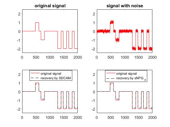
Figure 1: Recovery comparison for
noisy signal.

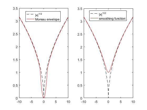
Figure 2: $|x|^{1/2}$ with its Moreau envelope and smoothing function.

To illustrate intuitively the approximation used in our SDCAM and sNPG, we plot the function $f(x)=|x|^{1/2}$ (in dashed lines), its Moreau envelope and its smoothing function in Figure 2. One can see that the envelope smooths the original nonsmooth point by a quadratic function. It is a lower approximation of $f$, while the smoothing function is an upper approximation of $f$.

5.2 Simultaneously sparse and low rank matrix optimization problem: which constraint should be modeled by $P_{1}$?

We consider the following special instance of simultaneously sparse and low rank matrix optimization problem:

$$\begin{array}[]{cl}\underset{\bm{X}}{\mbox{minimize}}&~{}\displaystyle\frac{1}{2}\|\bm{X}-\bm{M}\|_{F}^{2}\\ \mbox{subject to}&\|{\mbox{$\rm vec$}}(\bm{X})\|_{0}\leq s,~{}\displaystyle{\mbox{$\rm rank$}}(\bm{X})\leq k,\end{array}$$ (65)

where $\bm{M}\in\mathbb{R}^{m\times n}$ is a given noisy matrix, $s$ and $k$ are positive integers. Note that $f(\bm{X}):=\frac{1}{2}\|\bm{X}-\bm{M}\|_{F}^{2}$ is level-bounded. Therefore, (65) has at least one solution. Then, as discussed in Example 5, we can apply SDCAM to solving (65) in two different ways by considering, respectively, the two formulations in (58) and (60): the indicator function $\delta_{|\cdot|_{0}\leq s}(\cdot)$ is approximated by the Moreau envelope in (58) and the function $\delta_{{\mbox{$\rm rank$}}(\cdot)\leq k}(\cdot)$ is approximated by its Moreau envelope in (60). We call the method based on (58) SDCAM_r and the method based on (60) SDCAM_s. In the following experiments, we compare these two methods.

Data generation:

We first randomly generate $\bm{M}_{1}\in\mathbb{R}^{m\times k}$ and $\bm{M}_{2}\in\mathbb{R}^{k\times n}$ to have i.i.d. standard Gaussian entries. Then we set $m/10$ random rows of $\bm{M}_{1}$ to zero and let $\bm{M}=\bm{M}_{1}\bm{M}_{2}+\sigma\bm{\Delta}$, where $\sigma>0$ is a noise factor and $\bm{\Delta}$ has i.i.d. standard Gaussian entries. We fix $n=500$, $k=10$ and $s=mn/10$, and we experiment with $\sigma=0.005,0.01,0.02$ and $m=1000,2000,3000$ below.

Parameter setting:

In both SDCAM_r and SDCAM_s, we set $\lambda_{t}=1/10^{t+1}$ and $\bm{X}^{\rm feas}=\bm{0}$. In the NPG_major for solving the subproblems, we use the same parameter setting as in Section 5.1. We initialize both algorithms at $\bm{X}^{\rm feas}$ and terminate them when

$${\rm dist}(\bm{X}^{t},S)\leq 10^{-6}\cdot\|\bm{X}^{t}\|_{F}~{}~{}{\rm and}~{}~{}\ {\rm dist}(\bm{X}^{t},\Xi_{k})\leq 10^{-6}\cdot\|\bm{X}^{t}\|_{F},$$

respectively.

Numerical results:

In Table 2, we compare SDCAM_r and SDCAM_s in terms of the number of iterations (iter), CPU time (CPU) and the feasibility violation (vio) (i.e., ${\rm dist}(\bm{X}^{t},S)$ and ${\rm dist}(\bm{X}^{t},\Xi_{k})$, respectively) at termination, averaged over 10 randomly generated instances. One can see that SDCAM_r takes fewer iterations and less time. An intuitive explanation could be that the rank constraint is a more complicated constraint than the sparsity constraint to approximate via “subgradients”. Thus, the algorithm SDCAM_r that maintains all its iterates in the rank constraint and then attempts to approximately satisfy the sparsity constraint as the algorithm progresses ends up converging more quickly.

Table 2: Comparison of SDCAM_r and SDCAM_s for solving (65).

$\sigma$	$m$	iter		CPU		vio
		SDCAMr	SDCAMs	SDCAMr	SDCAMs	SDCAMr	SDCAMs
	1000	41	5597	4.7	378.1	4.7569e-04	1.0515e-04
0.005	2000	12	5298	4.0	647.0	6.7084e-04	1.5247e-04
	3000	12	4618	6.0	862.8	8.2038e-04	1.8857e-04
	1000	4508	7900	379.3	529.2	9.4347e-05	2.1032e-04
0.010	2000	4453	7526	653.6	912.6	1.3412e-04	3.0580e-04
	3000	4428	5721	969.5	1080.6	1.6434e-04	3.7701e-04
	1000	4922	11631	413.7	769.2	1.8985e-04	4.2222e-04
0.020	2000	4634	10267	675.5	1251.3	2.6849e-04	6.1136e-04
	3000	4580	10859	1003.5	2043.0	3.2804e-04	7.5510e-04

6 Conclusions

In this paper, we propose a successive difference-of-convex approximation method for solving (1). The key idea of this method is to approximate the nonsmooth functions in the objective of (1) by their Moreau envelopes. The approximation function can then be minimized by various proximal gradient methods with majorization techniques such as NPG_major in the appendix, thanks to (6). We prove that the sequence generated by our method is bounded and any accumulation point is a stationary point of (1) under suitable conditions. We also discuss how to apply our method to concrete applications and conduct numerical experiments to illustrate its efficiency.

Appendix A Convergence of an NPG method with majorization

In this appendix, we consider the following optimization problem:

$$\begin{array}[]{rl}\min\limits_{\bm{x}}&F(\bm{x})=h(\bm{x})+P(\bm{x})-g(\bm{x}),\end{array}$$ (66)

where $h$ is an $L_{h}$-smooth function, $P$ is a proper closed function with $\inf P>-\infty$ and $g$ is a continuous convex function. We assume in addition that there exists $\bm{x}^{0}\in{\rm dom}\,P$ so that $F$ is continuous in $\Omega(\bm{x}^{0}):=\{\bm{x}:\;F(\bm{x})\leq F(\bm{x}^{0})\}$ and the set $\Omega(\bm{x}^{0})$ is compact. As a consequence, it holds that $\inf F>-\infty$.

In Algorithm 2 below, we describe an algorithm, the nonmonotone proximal gradient method with majorization (NPG_major), for solving (66). We first show that the line-search criterion is well-defined.

Algorithm 2 The NPG_major for (66)

Step 0.

Choose $\bm{x}^{0}\in{\rm dom}\,P$ so that $\Omega(\bm{x}^{0})$ is compact and $F$ is continuous in it. Pick $L_{\max}\geq L_{\min}>0$, $\tau>1$, $c>0$ and an integer $M\geq 0$ arbitrarily. Set $t=0$.

Step 1.

Choose any $L^{0}_{t}\in[L_{\min},L_{\max}]$ and set $L_{t}=L^{0}_{t}$.

1. Pick any $\bm{\zeta}^{t}\in\partial g(\bm{x}^{t})$. Solve the subproblem

   $$\bm{u}\in\operatornamewithlimits{Argmin}_{\bm{x}}\left\{(\nabla h(\bm{x}^{t})-\bm{\zeta}^{t})^{\top}(\bm{x}-\bm{x}^{t})+\frac{L_{t}}{2}\|\bm{x}-\bm{x}^{t}\|^{2}+P(\bm{x})\right\}.$$ (67)

2. If

   $$F(\bm{u})\leq\max_{[t-M]_{+}\leq i\leq t}F(\bm{x}^{i})-\frac{c}{2}\|\bm{u}-\bm{x}^{t}\|^{2}$$ (68)

   is satisfied, then go to step 2).

3. Set $L_{t}\leftarrow\tau L_{t}$ and go to step 1a).

Step 2.

If a termination criterion is not met, set $\bar{L}_{t}=L_{t}$, $\bm{x}^{t+1}=\bm{u}$, $t=t+1$. Go to Step 1.

Proposition 1

For each $t$, the condition (68) is satisfied after at most

$$\tilde{n}:=\max\left\{\left\lceil\frac{\log(L_{h}+c)-\log(L_{\min})}{\log\tau}\right\rceil,1\right\}$$

inner iterations, which is independent of $t$. Consequently, $\{\bar{L}_{t}\}$ is bounded.

Proof

For each $t$ and $L>0$, let $\bm{u}^{t}_{L}$ be an arbitrarily fixed element in

$$\operatornamewithlimits{Argmin}_{\bm{x}}\left\{(\nabla h(\bm{x}^{t})-\bm{\zeta}^{t})^{\top}(\bm{x}-\bm{x}^{t})+\frac{L}{2}\|\bm{x}-\bm{x}^{t}\|^{2}+P(\bm{x})\right\}.$$

Then we have

$$\begin{split}F(\bm{u}^{t}_{L})&\leq h(\bm{x}^{t})+\nabla h(\bm{x}^{t})^{\top}(\bm{u}^{t}_{L}-\bm{x}^{t})+\frac{L_{h}}{2}\|\bm{u}^{t}_{L}-\bm{x}^{t}\|^{2}+P(\bm{u}^{t}_{L})-g(\bm{x}^{t})-{\bm{\zeta}^{t}}^{\top}(\bm{u}^{t}_{L}-\bm{x}^{t})\\ &=h(\bm{x}^{t})-g(\bm{x}^{t})+(\nabla h(\bm{x}^{t})-{\bm{\zeta}^{t}})^{\top}(\bm{u}^{t}_{L}-\bm{x}^{t})+\frac{L_{h}}{2}\|\bm{u}^{t}_{L}-\bm{x}^{t}\|^{2}+P(\bm{u}^{t}_{L})\\ &\leq F(\bm{x}^{t})+\frac{L_{h}-L}{2}\|\bm{u}^{t}_{L}-\bm{x}^{t}\|^{2},\end{split}$$

where the first inequality holds because of the $L_{h}$-smoothness of $h$, the convexity of $g$ and the fact that $\bm{\zeta}^{t}\in\partial g(\bm{x}^{t})$, and the last inequality follows from the definition of $\bm{u}^{t}_{L}$ as a minimizer. Thus, at the $t$-th iteration, the criterion (68) is satisfied by $\bm{u}=\bm{u}^{t}_{L}$ whenever $L\geq L_{h}+c$. Since we have

$$\tau^{\tilde{n}}L^{0}_{t}\geq\tau^{\tilde{n}}L_{\min}\geq L_{h}+c,$$

we conclude that (68) must be satisfied at or before the $\tilde{n}$-th inner iteration. Consequently, we have $\bar{L}_{t}\leq\tau^{\tilde{n}}L_{\max}$ for all $t$. $\Box$

The convergence of NPG_major can now be proved similarly as in (WrightNF09, , Lemma 4).

Proposition 2

Let $\{\bm{x}^{t}\}$ be the sequence generated by NPG_major. Then $\|\bm{x}^{t+1}-\bm{x}^{t}\|\to 0$.

References

- (1)
- (2) M. Ahn, J. S. Pang and J. Xin. Difference-of-convex learning: directional stationarity, optimality, and sparsity. SIAM Journal on Optimization, 27:1637–1665, 2017.
- (3) E. Asplund. Differentiability of the metric projection in finite dimensional Euclidean space. Proceedings of the American Mathematical Society, 38:218–219, 1973.
- (4) H. H. Bauschke and P. L. Combettes. Convex Analysis and Monotone Operator Theory in Hilbert Spaces. Springer 2011.
- (5) S. Becker, E. J. Candès and M. Grant. Templates for convex cone problems with applications to sparse signal recovery. Mathematical Programming Computation, 3:165–218, 2011.
- (6) R. Borsdorf, N. J. Higham and M. Raydan. Computing a nearest correlation matrix with factor structure. SIAM Journal on Matrix Analysis and Applications, 31:2603–2622, 2010.
- (7) J. Brodie, I. Daubechies, C. De Mol, D. Giannone and I. Loris. Sparse and stable Markowitz portfolios. Proceedings of the National Academy of Sciences, 106:12267–12272, 2009.
- Candès and Recht (2009) E. J. Candès and B. Recht. Exact matrix completion via convex optimization. Foundations of Computational Mathematics, 9:717–772, 2009.
- (9) C. Chen, X. Li, C. Tolman, S. Wang and Y. Ye. Sparse portfolio selection via quasi-norm regularization. ArXiv:1312.6350, 2013.
- (10) J. Eckstein and D. P. Bertsekas. On the Douglas-Rachford splitting method and the proximal point algorithm for maximal monotone operators Mathematical Programming, 55:293–318, 1992.
- (11) D. Gabay and B. Mercier. A dual algorithm for the solution of nonlinear variational problems via finite element approximations. Computers & Mathematics with Applications, 2:17-40, 1976.
- (12) Y. Gao and D. Sun. A majorized penalty approach for calibrating rank constrained correlation matrix problems, Technical report, National University of Singapore, 2010.
- Gong et al. (2013) P. Gong, C. Zhang, Z. Lu, J. Huang and J. Ye. A general iterative shrinkage and thresholding algorithm for non-convex regularized optimization problems. In Proceedings of the 30th International Conference on Machine Learning, 37–45, 2013.
- (14) G. Li and T. K. Pong. Global convergence of splitting methods for nonconvex composite optimization. SIAM Journal on Optimization, 25:2434–2460, 2015.
- (15) Z. Lu and X. Li. Sparse recovery via partial regularization: Models, theory and algorithms. ArXiv:1511.07293, 2015.
- (16) Z. Lu and Y. Zhang. Sparse approximation via penalty decomposition methods. SIAM Journal on Optimization, 23:2448–2478, 2013.
- (17) Z. Lu, Y. Zhang and X. Li. Penalty decomposition methods for rank minimization. Optimization Methods and Software, 30:531–558, 2015.
- (18) Y. Lucet. Fast Moreau envelope computation I: Numerical algorithms. Numerical Algorithms, 43:235–249, 2006.
- (19) I. Markovsky. Structured low-rank approximation and its applications. Automatica, 44: 891–909, 2008.
- (20) H. Markowitz. Portfolio selection. The Journal of Finance, 7:77–91, 1952.
- (21) Y. Nesterov. Smooth minimization of non-smooth functions. Mathematical Programming, 103:127–152, 2005.
- (22) A. Parekh and I. W. Selesnick. Convex fused Lasso denoising with non-convex regularization and its use for pulse detection. Proceedings of IEEE Signal Processing in Medicine and Biology Symposium, 1–6, 2015.
- (23) B. Recht, M. Fazel and P. A. Parrilo. Guaranteed minimum-rank solutions for linear matrix equations via nuclear norm minimization. SIAM Review, 52:471–501, 2010.
- Richard, et al. (2010) E. Richard, P.-A. Savalle and N. Vayatis. Estimation of simultaneously sparse and low rank matrices. ArXiv:1206.6474, 2012.
- (25) R. T. Rockafellar. Convex Analysis. Princeton University Press 1970.
- (26) R. T. Rockafellar and R. J-B. Wets. Variational Analysis. Springer 1998.
- Slawski and Hein (2013) M. Slawski and M. Hein. Non-negative least squares for high-dimensional linear models: Consistency and sparse recovery without regularization. Electronic Journal of Statistics, 7:3004–3056, 2013.
- Thiao et al. (2010) M. Thiao, D. T. Pham and H. A. Le Thi. A DC programming approach for sparse eigenvalue problem, Proceedings of the 27th International Conference on Machine Learning, 1063–1070, 2010.
- Tibshirani (1996) R. Tibshirani. Regression shrinkage and selection via the Lasso. Journal of the Royal Statistical Society B, 58:267–288, 1996.
- Tibshirani and Taylor (1996) R. Tibshirani and J. Taylor. The solution path of the generalized Lasso. The Annals of Statistics, 39:1335–1371, 2011.
- Tono et al. (2017) K. Tono, A. Takeda and J. Gotoh. Efficient DC algorithm for constrained sparse optimization. ArXiv:1701.08498, 2017.
- (32) S. J. Wright, R. D. Nowak and M. A. T. Figueiredo. Sparse reconstruction by separable approximation. IEEE Transactions on Signal Processing, 57:2479–2493, 2009.
- (33) Y. L. Yu. Better approximation and faster algorithm using the proximal average. Advances in Neural Information Processing Systems 26:458–466, 2013.
- (34) Y. L. Yu, X. Zheng, M. Marchetti-Bowick and E. Xing. Minimizing nonconvex non-separable functions. Proceedings of the 18th International Conference on Artificial Intelligence and Statistics 38:1107–1115, 2015.