Majorana Dark Matter in a new $B-L$ model

Abstract

We present a comprehensive study of Majorana dark matter in a $U(1)_{B-L}$ gauge extension of the standard model, where three exotic fermions with $B-L$ charges as $-4,-4,+5$ are added to make the model free from the triangle gauge anomalies. The enriched scalar sector and the new heavy gauge boson $Z^{\prime},$ associated with the $U(1)_{B-L}$ symmetry make the model advantageous to be explored in dual portal scenarios for the search of dark matter signal. Diagonalizing the exotic fermion mass matrix, we obtain the Majorana mass eigenstates, of which the lightest one plays the role of dark matter. Analyzing the effect of two mediators separately, the scalar portal channels give a viable parameter space consistent with relic density from PLANCK data and the direct detection limits from various experiments such as LUX, XENON1T and PandaX. While the $Z^{\prime}$ mediated channels are constrained from relic abundance and LHC searches for $Z^{\prime}$ in the dilepton channel. A massless physical Goldstone boson plays a key role in the scalar portal relic density. Finally, we briefly discuss the neutrino mass generation at one-loop level.

1 Introduction

Standard model (SM) of particle physics is the most successful theory that can explain well almost all the observed data below the electroweak scale. Still there are many open issues for which SM does not provide any satisfactory answer. Of these open questions, the one that stands out is the nature of Dark matter (DM). Various observational evidences firmly point towards the existence of dark matter which constitutes about $26.8\%$ energy budget of the Universe [1], still very little is known about its true nature. The DM has been the most sought after candidate for experimental particle physicists and the hunt for it started from the day of its existence, which was proposed way back in 1937 [2, 3]. Its nature to interact ‘weakly’ as confirmed indirectly from the Bullet cluster [4], provides strong motivation to prefer weakly interacting massive particles (WIMPs) as the potential DM candidates, which are not too far from the electroweak scale, thus, providing an excellent testing ground at the current or near future direct or indirect dark matter detection experiments.

To explain the key ingredient that connects cosmology with the particle physics, plenty of frameworks have been proposed imposing the condition that the DM is stable at the cosmological time scale. Apart from this, as the spin of DM is unknown, all possible kinds of DM candidates, i.e., scalar, fermion, vector have been explored. As SM is a well tested gauge theory, we intend to study the gauge extensions of it where the difference of Baryon and Lepton number $(B-L)$ is promoted to the local gauge symmetry [5, 6, 7, 8]. One of the interesting aspects is that in its standard form, the presence of right-handed neutrinos and the type-I seesaw mechanism for neutrino mass generation is natural. In particular, $B-L$ gauge extension of SM has been studied so as to incorporate the beyond Standard Model (BSM) physics (see some earlier works in this motivation [9, 10, 11, 12, 13, 14, 15, 16, 17, 18, 19, 20, 21, 22, 23]). In this article, we explore the prospects for Majorana DM in the context of $B-L$ gauge extensions of SM.

The model considered here consists of a particular $B-L$ charge assignment for the extra fields added to SM, such that there is an automatic cancellation of anomalies as well as the existence of a stable Majorana DM candidate [24, 25, 26, 27]. The model incorporates a scalar sector with two additional heavy scalars alongside the SM Higgs. In particular, one of the scalars carries a $B-L$ charge of $+8$ which gives rise to a scalar portal interaction with the Majorana DM candidate such that there can be observable signals. This is complemented by the usual $Z^{\prime}$ mediated interactions, where the Majorana DM couples to the $Z^{\prime}$. Thus, we have a Majorana DM that can interact with SM particles through two portals - one scalar and one vector. We shall study the phenomenology resulting from both these types of interactions using constraints from direct and indirect detection of DM, as well as collider searches for $Z^{\prime}$.

The paper is organized as follows. In section II, we discuss a new variant of $U(1)_{B-L}$ gauge extension of SM with three exotic fermions and an extended scalar sector. In section III, we give details of the masses and mixings in the fermion and scalar sectors after spontaneous symmetry breaking. Section IV discusses the dark matter phenomenology including relic density and direct constraints. Collider limits on the current model are investigated in section V. Discussion regarding the generation of neutrino mass is presented in section VI and finally we conclude in section VII.

2 New $B-L$ model with Majorana Dark Matter

We consider an anomaly free $U(1)_{B-L}$ gauge extension of the SM where three exotic neutral fermions with $B-L$ charges $-4,-4,+5$ are added to get rid of the non-trivial triangle gauge anomalies. This minimal charge assignment was first proposed in [28] and later explored in [24, 25]. Another possibility is to add four exotic fermions charged $4/3,1/3,-2/3$ and$-2/3$ under new $U(1)$, which was first put forth in Ref. [27] and later studied in dark matter context in [29]. However, we do not study the second possibility as it has already been studied in the dark matter context and due to the fact that our present choice requires the addition of only three fermions. In addition, two scalar singlets $\phi_{1}$ and $\phi_{8}$ are introduced to generate the mass terms for the exotic neutral fermions after the spontaneous breaking of $B-L$ gauge symmetry. Singlet dark matter in the similar context has been explored recently in [30].

	Field	$SU(2)_{L}\times U(1)_{Y}$	$U(1)_{B-L}$
Fermions	$Q_{L}\equiv(u,d)^{T}_{L}$	$(\textbf{2},~{}1/6)$	$1/3$
	$u_{R}$	$(\textbf{1},~{}2/3)$	$1/3$
	$d_{R}$	$(\textbf{1},~{}-1/3)$	$1/3$
	$\ell_{L}\equiv(\nu,~{}e)^{T}_{L}$	$(\textbf{2},~{}-1/2)$	$-1$
	$e_{R}$	$(\textbf{1},~{}-1)$	$-1$
	$N_{1R}$	$(\textbf{1},~{}0)$	$-4$
	$N_{2R}$	$(\textbf{1},~{}0)$	$-4$
	$N_{3R}$	$(\textbf{1},~{}0)$	$5$
Scalars	$H$	$(\textbf{2},~{}1/2)$	$0$
	$\phi_{1}$	$(\textbf{1},~{}0)$	$-1$
	$\phi_{8}$	$(\textbf{1},~{}0)$	$8$

Table 1: Fields and their charges of the proposed $U(1)_{B-L}$ model.

Using the particle content listed in Table  1, one can write the following invariant Lagrangian

$$\mathcal{L}_{\text{BL}} =-\frac{1}{3}\,g_{\text{BL}}\overline{Q}_{L}\,Z_{\mu}^{\prime}\gamma^{\mu}Q_{L}-\frac{1}{3}\,g_{\text{BL}}\overline{u}_{R}\,Z_{\mu}^{\prime}\gamma^{\mu}u_{R}-\frac{1}{3}\,g_{\text{BL}}\overline{d}_{R}\,Z_{\mu}^{\prime}\gamma^{\mu}d_{R}$$ (2.1)

$$~{}~{}~{}+\,g_{\text{BL}}\overline{\ell}_{L}\,Z_{\mu}^{\prime}\gamma^{\mu}\ell_{L}+\,g_{\text{BL}}\overline{e}_{R}\,Z_{\mu}^{\prime}\gamma^{\mu}e_{R}+i\,\overline{N}_{1R}\left(\not{\partial}+4i\,g_{\text{BL}}\,Z_{\mu}^{\prime}\gamma^{\mu}\right)\,N_{1R}$$

$$~{}~{}~{}+i\,\overline{N}_{2R}\left(\not{\partial}+4i\,g_{\text{BL}}\,Z_{\mu}^{\prime}\gamma^{\mu}\right)\,N_{2R}+i\,\overline{N}_{3R}\left(\not{\partial}-5i\,g_{\text{BL}}\,Z_{\mu}^{\prime}\gamma^{\mu}\right)\,N_{3R}$$

$$~{}~{}~{}-\frac{y_{\alpha\beta}}{2}\left(\sum_{\alpha,\beta=1,2}\overline{N^{c}_{\alpha R}}\,N_{\beta R}\,\phi_{8}+h.c.\right)-\frac{y_{\alpha 3}}{2}\left(\sum_{\alpha=1,2}\overline{N^{c}_{\alpha R}}\,N_{3R}\,\phi_{1}+h.c.\right)$$

$$~{}~{}~{}+|\left(\partial_{\mu}+\,i\,g_{\text{BL}}\,Z^{\prime}_{\mu}\right)\phi_{1}|^{2}+|\left(\partial_{\mu}-8\,i\,g_{\text{BL}}\,Z^{\prime}_{\mu}\right)\phi_{8}|^{2}$$

$$~{}~{}~{}-\frac{1}{4}F_{Z^{\prime}}^{\mu\nu}F^{Z^{\prime}}_{\mu\nu}+\frac{\kappa}{4}F_{Z^{\prime}}^{\mu\nu}\,F_{\mu\nu}-V\left(H,\phi_{1},\phi_{8}\right)+\mathcal{L}_{\text{SM}}\,,$$

where $Z_{\mu}^{\prime}$ is the new gauge boson associated with $B-L$ gauge symmetry. Also $F_{\mu\nu}^{Z^{\prime}}=\partial_{\mu}Z_{\nu}^{\prime}-\partial_{\nu}Z_{\mu}^{\prime}$ is the corresponding field strength tensor for $U(1)_{B-L}$. The term containing $\kappa$ is the kinetic mixing term between the two $U(1)$ gauge groups. However, electroweak measurements severely constrain the corresponding mixing angle to be $\leq 10^{-3}$ [31]. In the present work we neglect this small mixing.

The scalar potential of the model is given by

$$V(H,\phi_{1},\phi_{8})= \mu^{2}_{H}H^{\dagger}H+\lambda_{H}(H^{\dagger}H)^{2}+\mu^{2}_{1}\phi^{\dagger}_{1}\phi_{1}+\lambda_{1}(\phi^{\dagger}_{1}\phi_{1})^{2}+\mu^{2}_{8}\phi^{\dagger}_{8}\phi_{8}$$

$$+ \lambda_{8}(\phi^{\dagger}_{8}\phi_{8})^{2}+\lambda_{H1}(H^{\dagger}H)(\phi^{\dagger}_{1}\phi_{1})+\lambda_{H8}(H^{\dagger}H)(\phi^{\dagger}_{8}\phi_{8})$$

$$+ \lambda_{18}(\phi^{\dagger}_{1}\phi_{1})(\phi^{\dagger}_{8}\phi_{8}).$$ (2.2)

The stability of the scalar potential of the model is guaranteed by the co-positive criteria given by $\lambda_{H}\geq 0$, $\lambda_{1}\geq 0$, $\lambda_{8}\geq 0$, $\lambda_{H1}+\sqrt{\lambda_{H}\lambda_{1}}\geq 0$, $\lambda_{H8}+\sqrt{\lambda_{H}\lambda_{8}}\geq 0$, $\lambda_{18}+\sqrt{\lambda_{1}\lambda_{8}}\geq 0,\sqrt{\lambda_{H}\lambda_{1}\lambda_{8}}+\lambda_{H1}\sqrt{\lambda_{8}}+\lambda_{H8}\sqrt{\lambda_{1}}+\lambda_{18}\sqrt{\lambda_{H}}\geq 0$. Tree level perturbative unitarity constrain the scalar couplings as

$$\lambda_{H},\lambda_{1},\lambda_{8}\leq 4\pi/3,$$

$$\lambda_{H1},\lambda_{H8},\lambda_{18}\leq 4\pi.$$ (2.3)

3 Spontaneous symmetry breaking, masses and mixing

The spontaneous symmetry breaking of $SU(2)_{L}\times U(1)_{Y}\times U(1)_{B-L}$ down to SM gauge group $SU(2)_{L}\times U(1)_{Y}$ is implemented with the scalars $\phi_{1}$ and $\phi_{8}$. Then the spontaneous symmetry breaking of SM gauge group to low energy theory is achieved by assigning a non-zero VEV to SM Higgs doublet. Similar kind of $B-L$ model with additional scalars with $\phi_{1}$ and $\phi_{2}$ has been discussed in Ref [27], which avoids the presence of any accidental global $U(1)$ symmetry because of cross term $\mu\left({\phi^{2}}^{\dagger}_{1}\phi_{2}+\phi^{2}_{1}\phi^{\dagger}_{2}\right)$. However, in our model gauge invariance forbids the inclusion of such cross terms between $\phi_{1}$ and $\phi_{8}$, leading to an accidental global symmetry. As a result, after spontaneous symmetry breaking two massless Goldstone modes arise such that one linear combination of them will be eaten up by the neutral gauge boson corresponding to $U(1)_{B-L}$ gauge group and gives mass to $Z^{\prime}$ and the other orthogonal combination remains as massless Goldstone boson. We shall discuss the implications for this massless Goldstone boson in subsequent discussions.

The neutral components of the fields $H$, $\phi_{1}$ and $\phi_{8}$ can be parametrised in terms of real scalars and pseudoscalars as

$$H^{0}=\frac{1}{\sqrt{2}}(v+h)+\frac{i}{\sqrt{2}}A^{0}\,,$$

$$\phi_{1}=\frac{1}{\sqrt{2}}(v_{1}+h_{1})+\frac{i}{\sqrt{2}}A_{1}\,,$$

$$\phi_{8}=\frac{1}{\sqrt{2}}(v_{8}+h_{8})+\frac{i}{\sqrt{2}}A_{8}\,.$$

Here the VEVs of the scalars are given as $\langle H\rangle=(0,v/\sqrt{2})^{T}$, $\langle\phi_{1}\rangle=v_{1}/\sqrt{2}$, $\langle\phi_{8}\rangle=v_{8}/\sqrt{2}$. Then, the CP-even scalar mass matrix can be written as

$$M_{0}^{2}=\begin{pmatrix}2\lambda_{H}v^{2}&\lambda_{H1}vv_{1}&\lambda_{H8}vv_{8}\\ \lambda_{H1}vv_{1}&2\lambda_{1}v_{1}^{2}&\lambda_{18}v_{1}v_{8}\\ \lambda_{H8}vv_{8}&\lambda_{18}v_{1}v_{8}&2\lambda_{8}v_{8}^{2}\\ \end{pmatrix}.$$ (3.1)

We consider the Higgs doublet $H$ mixes equally with the two singlets and the mixing is minimal so that the Higgs decay width is consistent with LHC limits. We also assume the VEVs of the singlets $v_{1}\simeq v_{8}\gg v$ and the couplings $\lambda_{1}\simeq\lambda_{8}$, $\lambda_{H1,H8}\ll\lambda_{H}$, then the mass matrix can have the form

$$M_{0}^{2}\simeq\begin{pmatrix}~{}a~{}&~{}a~{}&~{}a~{}\\ ~{}a~{}&~{}y~{}&~{}b~{}\\ ~{}a~{}&~{}b~{}&~{}y~{}\\ \end{pmatrix}.$$ (3.2)

In the limit of minimal Higgs mixing, the unitary matrix connecting flavor and mass eigenstates takes the form

$$U\simeq\begin{pmatrix}1&~{}\beta\cos\alpha-\beta\sin\alpha&~{}\beta\cos\alpha+\beta\sin\alpha\\ -\beta&~{}\cos\alpha&~{}\sin\alpha\\ -\beta&~{}-\sin\alpha&~{}\cos\alpha\\ \end{pmatrix},$$ (3.3)

where $\beta=\frac{a}{b+y-a}$denotes the mixing between $H-\phi_{1,8}$ and $\alpha=\frac{5\pi}{4}$ is the mixing parameter for $\phi_{1}-\phi_{8}$, which are obtained from the normalized eigenvector matrix of $M_{0}^{2}$ (3.2). Thus, we obtain the relation between flavor and mass eigenstates as

$$\begin{pmatrix}h\\ h_{1}\\ h_{8}\\ \end{pmatrix}=U\begin{pmatrix}H_{1}\\ H_{2}\\ H_{3}\end{pmatrix}=\begin{pmatrix}H_{1}-H_{3}\beta\sqrt{2}\\ -H_{1}\beta-\frac{H_{2}}{\sqrt{2}}-\frac{H_{3}}{\sqrt{2}}\\ -H_{1}\beta+\frac{H_{2}}{\sqrt{2}}-\frac{H_{3}}{\sqrt{2}}\\ \end{pmatrix}.$$ (3.4)

The various scalar couplings can be expressed as

$$2\lambda_{H}v^{2}=\lambda_{H1}vv_{1}=\lambda_{H8}vv_{8}=\frac{M_{H_{1}}^{2}}{(1-2\beta+2\beta^{2})},$$

$$2\lambda_{1}v_{1}^{2}=2\lambda_{8}v_{8}^{2}=\frac{(\beta+1)M_{H_{3}}^{2}+(1+\beta+4\beta^{2})M_{H_{2}}^{2}}{2(1+\beta+4\beta^{2})},$$

$$\lambda_{18}v_{1}v_{8}=\frac{(\beta+1)M_{H_{3}}^{2}-(1+\beta+4\beta^{2})M_{H_{2}}^{2}}{2(1+\beta+4\beta^{2})}.$$ (3.5)

Here $H_{1}$ denotes the SM Higgs with $M_{H_{1}}=125.09$ GeV and $v=246$ GeV. As discussed earlier, $A_{\rm G}$ appears as the longitudinal polarization of $Z^{\prime}$ and the physical massless Goldstone, $A_{\rm NG}$ are given by

$$A_{\rm G}=-\frac{8v_{8}}{\sqrt{v_{1}^{2}+64v_{8}^{2}}}A_{8}+\frac{v_{1}}{\sqrt{v_{1}^{2}+64v_{8}^{2}}}A_{1},$$

$$A_{\rm NG}=\frac{v_{1}}{\sqrt{v_{1}^{2}+64v_{8}^{2}}}A_{8}+\frac{8v_{8}}{\sqrt{v_{1}^{2}+64v_{8}^{2}}}A_{1}.$$ (3.6)

As per the assumption $v_{1}\simeq v_{8}$, one can see that $A_{\rm G}$ gets major contribution from $A_{8}$ and $A_{\rm NG}$ is maximally composed of $A_{1}$. It should be noted that the massless mode ($A_{\rm NG})$ doesn’t couple to any SM particle except Higgs, as we considered non-zero mixing between $H$ and new scalars. It can give rise to an additional decay channel contributing to the invisible width of SM Higgs, given as

$$\Gamma(H_{1}\to A_{\rm NG}A_{\rm NG})\simeq\frac{M_{H_{1}}^{3}\sin^{2}\beta}{32\pi}\left(\frac{v_{1}^{3}+64v_{8}^{3}}{v_{1}v_{8}(v_{1}^{2}+64v_{8}^{2})}\right)^{2}~{}.$$ (3.7)

The invisible branching ratio of Higgs is given as

$$\text{Br}_{\rm inv}=\frac{\Gamma(H_{1}\to A_{\rm NG}A_{\rm NG})}{\Gamma(H_{1}\to A_{\rm NG}A_{\rm NG})+\cos^{2}\beta~{}\Gamma^{\rm Higgs}_{\rm SM}}.$$ (3.8)

Using the constraint, $\text{Br}_{\rm inv}\simeq 20\%$ [32, 33], $\Gamma^{\rm Higgs}_{\rm SM}\simeq 4$ MeV, we obtain the upper limit on the mixing angle as

$$|{\tan\beta}|\lesssim 2.2\times 10^{-4}\times\left(\frac{v_{1}}{\text{GeV}}\right).$$ (3.9)

Moreover, if the NG stays in thermal equilibrium with ordinary matter until muon annihilation, then it mimics as fractional cosmic neutrinos contributing nearly 0.39 to the effective number of neutrino species [34, 35] to give $N_{\rm eff}=3.36^{+0.68}_{-0.64}$ at $95\%$ C.L, a remarkable agreement with Planck data [36]. This illustration was done by working in the low mass regime of the physical scalar ($\simeq 500$ MeV) [34]. However, in [35] it was found that for masses $\gtrsim$ 4 GeV the Goldstone bosons do not contribute to $N_{\rm eff}$. And since in the present work we consider higher mass regime for the physical scalar spectrum to discuss the effect of NG on relic density, the contribution of NG to $N_{\rm eff}$ is not applicable.

3.1 Mixing in fermion sector

The heavy Majorana mass matrix is given by

$$M_{R}=\begin{pmatrix}y_{11}\langle\phi_{8}\rangle&y_{12}\langle\phi_{8}\rangle&y_{13}\langle\phi_{1}\rangle\\ y_{12}\langle\phi_{8}\rangle&y_{22}\langle\phi_{8}\rangle&y_{23}\langle\phi_{1}\rangle\\ y_{13}\langle\phi_{1}\rangle&y_{23}\langle\phi_{1}\rangle&0\\ \end{pmatrix}\;.$$ (3.10)

For simplicity, we consider the above mass matrix with real entries of the form¹

$$M_{R}=\begin{pmatrix}x~{}&~{}a~{}&~{}b\\ a~{}&~{}x~{}&~{}b\\ b~{}&~{}b~{}&~{}0\\ \end{pmatrix},$$ (3.11)

which can be obtained by assuming the Yukawa couplings to satisfy the relations $y_{11}\approx y_{22}$ and $y_{13}\approx y_{23}$ along with $v_{1}\approx v_{8}$. The above mass matrix can be diagonalized using the unitary matrix as $(U_{1}\cdot K)^{T}\cdot M_{R}\cdot(U_{1}\cdot K)$, where $U_{1}$ is the normalized eigenvector matrix of $M_{R}$ and $K={\rm{diag}}(1,i,1)$ is a diagonal phase matrix used to avoid the negative mass eigenvalues. Thus, one obtains the mass matrix in the diagonal basis $M^{\rm diag}={\rm{diag}}(M_{D1},M_{D2},M_{D3})$ as

$$M^{\rm diag}=\begin{pmatrix}x-a&0&0\\ 0&\frac{1}{2}\left(-(x+a)+\sqrt{8b^{2}+(x+a)^{2}}\right)&0\\ 0&0&\frac{1}{2}\left((x+a)+\sqrt{8b^{2}+(x+a)^{2}}\right)\\ \end{pmatrix}.$$ (3.12)

To make the analysis simpler, we consider $M_{D2}=\frac{1}{2}M_{D3}$, which implies $b=x+a$. Thus, the final diagonal matrix is given by

$${\rm{diag}}(M_{D1},M_{D2},M_{D3})=\begin{pmatrix}x-a&0&0\\ 0&x+a&0\\ 0&0&2(x+a)\\ \end{pmatrix}.$$ (3.13)

Considering $x>a$, we get positive eigenvalues and the mass eigenstates $N_{Di}$ can be written as

$$N_{D1} = \frac{N_{\text{2}}-N_{\text{1}}}{\sqrt{2}},$$

$$N_{D2} = \frac{i\left(N_{\text{1}}+N_{\text{2}}-2N_{\text{3}}\right)}{\sqrt{6}},$$

$$N_{D3} = \frac{N_{\text{1}}+N_{\text{2}}+N_{\text{3}}}{\sqrt{3}}.$$ (3.14)

The Yukawa couplings can be expressed in terms of the physical masses as

$$y_{11} = y_{22}=\frac{\sqrt{2}~{}(M_{D1}+M_{D2})}{2v_{8}}\;,$$

$$y_{12} = \frac{\sqrt{2}~{}(-M_{D1}+M_{D2})}{2v_{8}}\;,$$

$$y_{13} = y_{23}=\frac{\sqrt{2}~{}M_{D2}}{v_{1}}\;.$$ (3.15)

The interaction terms between the new fermions and the $Z^{\prime}$ gauge boson can be written in the mass eigenstate basis as

$${\cal L}^{V}_{N_{Di}} = g_{BL}\biggr{[}-4\overline{N^{c}_{D1}}\gamma^{\mu}N_{D1}+2\overline{N^{c}_{D2}}\gamma^{\mu}N_{D2}-\overline{N^{c}_{D3}}\gamma^{\mu}N_{D3}$$ (3.16)

$$- 3i\sqrt{2}~{}\overline{N^{c}_{D2}}\gamma^{\mu}N_{D3}+3i\sqrt{2}~{}\overline{N^{c}_{D3}}\gamma^{\mu}N_{D2}\biggr{]}Z^{\prime}_{\mu}\;.$$

Similarly, the interaction terms with the singlets $\phi_{1}$ and $\phi_{8}$ are

$${\cal L}^{S}_{N_{Di}} = (y_{11}-y_{12})\overline{N^{c}_{D1}}\,N_{D1}\,\phi_{8}+\frac{1}{3}\left(4y_{13}\overline{N^{c}_{D2}}\,N_{D2}\phi_{1}-(y_{11}+y_{12})\overline{N^{c}_{D2}}\,N_{D2}\phi_{8}\right)$$ (3.17)

$$+ \frac{2}{3}\left(2y_{13}\overline{N^{c}_{D3}}\,N_{D3}\phi_{1}+(y_{11}+y_{12})\overline{N^{c}_{D3}}\,N_{D3}\phi_{8}\right)$$

$$+ \frac{2\sqrt{2}i}{3}\left(y_{13}\overline{N^{c}_{D2}}\,N_{D3}\phi_{1}-(y_{11}+y_{12})\overline{N^{c}_{D2}}\,N_{D3}\phi_{8}\right).$$

A glance at Eqns. (3.13), and (3.14) confirms that $N_{D1}$ is the lightest Majorana mass eigenstate and we intend to perform a detailed study of Majorana dark matter in this work.

4 Dark Matter phenomenology

Since the proposed dark matter particle $N_{D1}$, the lightest of the three Majorana states, which can interact with the scalar sector and vector gauge boson $Z^{\prime}$, the model can be well explored in dark matter observables in this dual portal scenarios separately. In this section, we will be discussing the DM phenomenology in our model. We begin our discussion with relic density constraints on Majorana dark matter in the $B-L$ model considered here.

4.1 Relic density for Majorana dark matter

We first present the analytical expressions for annihilation cross sections that contribute to relic density in our model.

The formula used for computing the relic abundance of dark matter is

$$\Omega\text{h}^{2}=\frac{2.14\times 10^{9}~{}{\rm{GeV}}^{-1}}{{g_{\ast}}^{1/2}M_{\rm{pl}}}\frac{1}{J(x_{f})}\;,$$ (4.1)

where the Planck mass $M_{\rm{pl}}=1.22\times 10^{19}~{}\rm{GeV}$, $g_{\ast}=106.75$ being the total number of effective relativistic degrees of freedom, and $J(x_{f})$ reads as

$$J(x_{f})=\int_{x_{f}}^{\infty}\frac{dx}{x^{2}}\langle\sigma v\rangle(x).$$ (4.2)

The freeze out parameter $x_{f}$ in the above integral is given as

$$x_{f}=\ln\left(\frac{0.038\ g\ M_{\text{Pl}}\ M_{D1}\ \langle\sigma v\rangle(x_{f})}{({g_{\ast}x_{f}})^{1/2}}\right),$$ (4.3)

where $g$ is the count of number of degrees of freedom of the dark matter particle. The thermally averaged annihilation cross section $\langle\sigma v\rangle$ is given by

$$\langle\sigma v\rangle(x)=\frac{x}{8M_{D1}^{5}K_{2}^{2}(x)}\int_{4M_{D1}^{2}}^{\infty}ds\>\hat{\sigma}\times(s-4M_{D1}^{2})\ \sqrt{s}\ K_{1}\left(\frac{x\sqrt{s}}{M_{D1}}\right),$$ (4.4)

where $K_{1}$, $K_{2}$ denote the modified Bessel functions and $x=M_{D1}/T$, with $T$ being the temperature. We now discuss the different annihilation channels that contribute to the relic density and the impact of the different parameters in both scalar and vector mediated DM scenarios.

4.1.1 Scalar mediated

(a)

(b)

(c)

(d)

(e)

(f)

Figure 1: Feynman diagrams contributing to relic density are shown in Figs. (a) - (e) while Fig. (f) is relevant for the direct searches.

The possible annihilation channels that can drive the relic density in the scalar portal scenario are shown in the first five Feynman diagrams of Fig. 1. These channels can be either SM fermions, SM gauge bosons ($W,Z$), Higgs sector scalars and the massless physical Goldstone mode. The cross section for the annihilation channels into SM fermions and gauge bosons are given by

$$\hat{\sigma}^{S}_{ff}= \frac{C}{v^{2}s}|F_{1}|^{2}\sum_{f}M^{2}_{f}c_{f}(s-4M^{2}_{f})(s-4M^{2}_{D1})\frac{(s-4M^{2}_{f})^{\frac{1}{2}}}{(s-4M^{2}_{D1})^{\frac{1}{2}}}\;,$$ (4.5)

$$\hat{\sigma}^{S}_{WW}= \frac{Cs}{2v^{2}}|F_{1}|^{2}(s-4M^{2}_{D1})\left(1-\frac{4M^{2}_{W}}{s}+\frac{12M^{4}_{W}}{s^{2}}\right)\frac{(s-4M^{2}_{W})^{\frac{1}{2}}}{(s-4M^{2}_{D1})^{\frac{1}{2}}}\;,$$ (4.6)

$$\hat{\sigma}^{S}_{ZZ}= \frac{Cs}{4v^{2}}|F_{1}|^{2}(s-4M^{2}_{D1})\left(1-\frac{4M^{2}_{Z}}{s}+\frac{12M^{4}_{Z}}{s^{2}}\right)\frac{(s-4M^{2}_{Z})^{\frac{1}{2}}}{(s-4M^{2}_{D1})^{\frac{1}{2}}}\;,$$ (4.7)

while the expressions for channels with NG in final state turn out to be

$$\hat{\sigma}^{S}_{\rm{NG}}= \frac{Cs}{4v_{1}^{2}v_{8}^{2}(v_{1}^{2}+64v_{8}^{2})^{2}}|F_{2}|^{2}(s-4M^{2}_{D1})\frac{s^{\frac{1}{2}}}{(s-4M^{2}_{D1})^{\frac{1}{2}}}\;,$$ (4.8)

$$\hat{\sigma}^{S}_{\rm{NG~{}H_{1}}}= \frac{C\beta^{2}}{2v_{8}^{2}(v_{1}^{2}+64v_{8}^{2})^{3}}\left(v_{1}^{3}+64v_{8}^{3}\right)^{2}\frac{(s-4M^{2}_{D1})^{\frac{1}{2}}(s-M_{H_{1}}^{2})^{3}}{s^{\frac{7}{2}}}\;,$$ (4.9)

$$\hat{\sigma}^{S}_{\rm{NG~{}H_{2}}}= \frac{C}{4v_{8}^{2}(v_{1}^{2}+64v_{8}^{2})^{3}}\left(v_{1}^{3}-64v_{8}^{3}\right)^{2}\frac{(s-4M^{2}_{D1})^{\frac{1}{2}}(s-M_{H_{2}}^{2})^{3}}{s^{\frac{7}{2}}}\;,$$ (4.10)

$$\hat{\sigma}^{S}_{\rm{NG~{}H_{3}}}= \frac{C}{4v_{8}^{2}(v_{1}^{2}+64v_{8}^{2})^{3}}\left(v_{1}^{3}+64v_{8}^{3}\right)^{2}\frac{(s-4M^{2}_{D1})^{\frac{1}{2}}(s-M_{H_{3}}^{2})^{3}}{s^{\frac{7}{2}}}\;,$$ (4.11)

where

$$C= \frac{(y_{11}-y_{12})^{2}}{8\pi}\;,$$ (4.12)

$$F_{1}= -\frac{\beta}{\left[(s-M^{2}_{H_{1}})+iM_{H_{1}}\Gamma_{H_{1}}\right]}+\frac{\beta}{\left[(s-M^{2}_{H_{3}})+iM_{H_{3}}\Gamma_{H_{3}}\right]}\;,$$ (4.13)

$$F_{2}= \frac{\beta^{2}\left(v_{1}^{3}+64v_{8}^{3}\right)}{\left[(s-M^{2}_{H_{1}})+iM_{H_{1}}\Gamma_{H_{1}}\right]}+\frac{1/2\left(v_{1}^{3}-64v_{8}^{3}\right)}{\left[(s-M^{2}_{H_{2}})+iM_{H_{2}}\Gamma_{H_{2}}\right]}+\frac{1/2\left(v_{1}^{3}+64v_{8}^{3}\right)}{\left[(s-M^{2}_{H_{3}})+iM_{H_{3}}\Gamma_{H_{3}}\right]}\;,$$ (4.14)

with $c_{f}$ and $M_{f}$ denoting the color charge and mass of the the SM fermion $f$ respectively. Finally, the Higgs sector annihilation channels we have

$$\hat{\sigma}^{S}_{H_{i}H_{j}}=\frac{C}{2s~{}n!}|F_{ij}|^{2}(s-4M^{2}_{D1})\frac{\left[(s-(M_{H_{i}}+M_{H_{j}})^{2})(s-(M_{H_{i}}-M_{H_{j}})^{2})\right]^{\frac{1}{2}}}{\left[s(s-4M^{2}_{D1})\right]^{\frac{1}{2}}}\;,$$ (4.15)

where

$$F_{ij}= -\frac{\lambda_{1ij}\beta}{\left[(s-M^{2}_{H_{1}})+iM_{H_{1}}\Gamma_{H_{1}}\right]}+\frac{\lambda_{2ij}/\sqrt{2}}{\left[(s-M^{2}_{H_{2}})+iM_{H_{2}}\Gamma_{H_{2}}\right]}-\frac{\lambda_{3ij}/\sqrt{2}}{\left[(s-M^{2}_{H_{3}})+iM_{H_{3}}\Gamma_{H_{3}}\right]}\;,$$

where $n$ denotes the permutation factor for identical final state particles and $\lambda_{1ij},\lambda_{2ij},\lambda_{3ij}$ having mass dimension denote the trilinear scalar couplings with $i,j=1,2,3$. In the analysis, we consider the VEVs $v_{1}$ and $v_{8}$ to be in TeV scale range so that the scalar couplings (3.5) are within the limits of unitarity bounds (2.3). The mixing parameter $\beta$ can be written in terms of the physical scalar masses as

$$\beta=\frac{-M_{H_{1}}^{2}+M_{H_{3}}^{2}-\sqrt{-15M_{H_{1}}^{4}-10M_{H_{3}}^{2}M_{H_{1}}^{2}+M_{H_{3}}^{4}}}{4\left(2M_{H_{1}}^{2}+M_{H_{3}}^{2}\right)}.$$ (4.16)

Since the Higgs mass ($M_{H_{1}}$) is fixed, the mass parameter $M_{H_{3}}$ defines the amount of mixing i.e., say $M_{H_{3}}\geq 1$ TeV implies $\beta\leq 0.016$. Fig. 2 displays the behavior of relic density with the dark matter mass where the PLANCK limit is reached on the either side of resonance of the propagators. For lower DM mass region, the channels $f\bar{f}$ and $A_{\rm NG}A_{\rm NG}$ maximally contribute to relic density. Then, the rest of channels contribute to relic density once they get kinematically allowed. The channels with $H_{1}H_{1}$ and $A_{\rm NG}A_{\rm NG}$ in final state can give the resonance in $H_{2}$ propagator. Emphasis is given more to the mass of $H_{3}$ as the WIMP-nucleon cross section also involves this mass parameter.

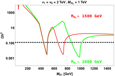
Figure 2: Scalar-portal relic abundance as a function of DM mass $M_{D1}$ for two specific mass values of the physical scalar $H_{3}$. The horizontal dashed lines represent the $3\sigma$ value of the current relic density [1].

4.1.2 Vector mediated

The DM also interacts with the visible sector through the gauge mediated processes which can lead to annihilation channels into SM fermions and the Higgs sector as shown in Fig. 3. The cross sections are given by

$$\hat{\sigma}^{V}_{ff}= \sum_{f}\frac{16(n^{f}_{\rm BL})^{2}g^{4}_{\rm BL}c_{f}|F_{V}|^{2}}{3\pi s}(s-4M^{2}_{D1})(s+2M^{2}_{f})\frac{(s-4M^{2}_{f})^{\frac{1}{2}}}{(s-4M^{2}_{D1})^{\frac{1}{2}}}\;,$$

$$\hat{\sigma}^{V}_{Z^{\prime}H_{3}}= \frac{4(64v_{8}+v_{1})^{2}g_{BL}^{6}|F_{V}|^{2}}{\pi s}\frac{((s-(M_{Z^{\prime}}+M_{H_{3}})^{2})(s-(M_{Z^{\prime}}-M_{H_{3}})^{2}))^{\frac{1}{2}}}{(s(s-4M^{2}_{D1}))^{\frac{1}{2}}}C_{H_{3}}\;,$$

$$\hat{\sigma}^{V}_{Z^{\prime}H_{2}}= \frac{4(64v_{8}-v_{1})^{2}g_{BL}^{6}|F_{V}|^{2}}{\pi s}\frac{((s-(M_{Z^{\prime}}+M_{H_{2}})^{2})(s-(M_{Z^{\prime}}-M_{H_{2}})^{2}))^{\frac{1}{2}}}{(s(s-4M^{2}_{D1}))^{\frac{1}{2}}}C_{H_{2}}\;,$$

$$\hat{\sigma}^{V}_{Z^{\prime}H_{1}}= \frac{8(64v_{8}+v_{1})^{2}\beta^{2}g_{BL}^{6}|F_{V}|^{2}}{\pi s}\frac{((s-(M_{Z^{\prime}}+M_{H_{1}})^{2})(s-(M_{Z^{\prime}}-M_{H_{1}})^{2}))^{\frac{1}{2}}}{(s(s-4M^{2}_{D1}))^{\frac{1}{2}}}C_{H_{1}}\;,$$ (4.17)

where

$$F_{V}= \frac{1}{\left[(s-M^{2}_{Z^{\prime}})+iM_{Z^{\prime}}\Gamma_{Z^{\prime}}\right]}\;,$$

$$C_{S}= \left[\frac{(s-8M_{D1}^{2})}{4}+\frac{1}{M_{Z^{\prime}}^{2}}\left(2sM_{D1}^{2}+\frac{(s+M_{Z^{\prime}}^{2}-M_{S}^{2})^{2}}{4}\right.\right.$$

$$\left.\left.-\frac{1}{48s}(s-4M_{D1}^{2})(s-(M_{Z^{\prime}}+M_{S})^{2})(s-(M_{Z^{\prime}}-M_{S})^{2})\right)\right],$$

Figure 3: Feynman diagrams contributing to relic density in the vector-mediated case.

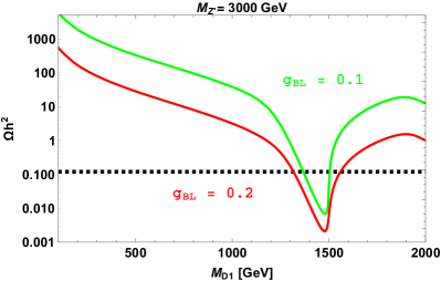
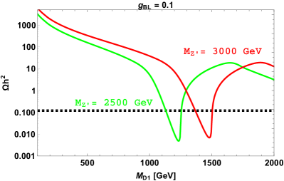
Figure 4: Variation of relic abundance $\Omega\text{h}^{2}$ with the mass of DM with $(M_{H_{2}},M_{H_{3}})=(1,1.5)$ TeV. Left panel depicts the variation for fixed $Z^{\prime}$ mass and varying $B-L$ gauge coupling $g_{BL}$. The right panel displays the behavior for constant coupling $g_{BL}$ and varying mediator mass. Here, the horizontal dashed lines represent the $3\sigma$ value of the current relic density [1].

with $S=H_{1},H_{2},H_{3}$. Here $n^{f}_{\rm BL}$ denotes the $B-L$ charge for the SM fermion $f$ and $\Gamma_{Z^{\prime}}$ is the decay width of the heavy gauge mediator $Z^{\prime}$. We use the packages LanHEP [37], micrOMEGAs [38, 39, 40] to compute the DM observables. Fig. 4 shows the behaviour of relic abundance with the mass of dark matter particle for various sets of gauge coupling $g_{BL}$ and the mediator mass $M_{Z^{\prime}}$ consistent with the LEP-II bound [41] i.e., $M_{Z^{\prime}}/g_{BL}>7$ TeV. Near the resonance the major contribution comes from the $N_{D1}N_{D1}\rightarrow f\bar{f}$ channel. As we go towards high mass regime of $M_{D1}$, the channels $N_{D1}N_{D1}\rightarrow Z^{\prime}H_{1,2,3}$ become dominant resulting in a slight decrease in the relic abundance.

4.2 Direct searches

In this section, we discuss the direct detection prospects for our model in both scalar and vector mediated DM scenarios. Since the vector boson $Z^{\prime}$ couples differently to Majorana fermion and quarks i.e., axial vector and vector type, the contribution by WIMP-nucleon interaction is insensitive to direct detection experiments [42, 43, 44]. Hence, we shall only focus on the scalar mediated DM scattering and constraints on it from various experiments. The effective Lagrangian term of scalar mediated channel shown in panel of Fig. 1-(f) that contributes to the spin-independent (SI) cross section for direct detection is

$$\mathcal{L}_{\mathrm{eff}}=a_{q}\overline{N}_{D1}N_{D1}\bar{q}q,$$ (4.18)

where

$$\frac{a_{q}}{M_{q}}=\frac{(y_{11}-y_{12})\beta}{\sqrt{2}v}\left(\frac{1}{M^{2}_{H_{3}}}-\frac{1}{M^{2}_{H_{1}}}\right).$$ (4.19)

The WIMP-nucleon SI contribution reads as

$$\sigma_{\rm SI}=\frac{4}{\pi}\left(\frac{M_{p}M_{D1}}{M_{p}+M_{D1}}\right)^{2}f_{p}^{2}\;,$$ (4.20)

where $M_{p}$ denotes the mass of proton and the hadronic matrix element $f_{p}$ is given as

$$\frac{f_{p}}{M_{p}}=\sum_{q=u,d,s}f_{Tq}^{p}\frac{a_{q}}{M_{q}}+\frac{2}{27}\left(1-\sum_{q=u,d,s}f_{Tq}^{p}\right)\sum_{q=c,b,t}\frac{a_{q}}{M_{q}}\;.$$ (4.21)

Typical values for proton are $f_{Tu}^{p}=0.020\pm 0.004$, $f_{Td}^{p}=0.026\pm 0.005$ and $f_{Ts}^{p}=0.118\pm 0.062$ [45].

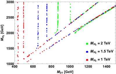
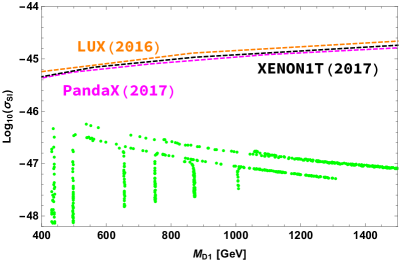
Figure 5: Left panel shows the parameter space satisfying the $3\sigma$ range in current relic density and the most stringent PandaX limit. Right panel depicts WIMP-nucleon cross section for the parameters space depicted in the left panel. The dashed lines denote the upper bound on SI cross section from LUX [46], XENON1T [47] and PandaX [48].

.

Parameters	Range
$v_{1,8}$ [GeV]	$2000$
$M_{H_{2}}$ [GeV]	$1000-2000$
$M_{H_{3}}$ [GeV]	$M_{H_{2}}-3000$
$\beta$	$0.016-0.0016$

Table 2: Parameters and their ranges for scalar portal analysis.

Varying the parameters in the range shown in Table. 2, we show in Fig. 5 (left panel), the parameter space that satisfies the $3\sigma$ range in the current relic density [1] and the PandaX limit [48]. Since the mixing parameter $\beta$ is small, the direct detection limits on the parameter space is not stringent. It is mainly constrained by relic density where the PLANCK limit is met near the resonance in two propagators $H_{2}$ (vertical data points) and $H_{3}$ (diagonal data points). Right panel depicts the WIMP-nucleon cross section with varying mass of the DM of the parameter space shown in the left panel.

5 Collider studies

In recent past, both ATLAS and CMS experiments have provided extensive studies to search for new heavy resonances in both dilepton and dijet signals. It is found that these two experiments provide lower limit on ${Z^{\prime}}$-boson with dileptons, resulting in stronger bounds than dijets due to relatively fewer background events. ATLAS results [49] from the study of dilepton signals for the $Z^{\prime}$ boson provide the most stringent limits on the heavy gauge boson mass $M_{Z^{\prime}}$ and the gauge coupling $g_{BL}$.

For the present $B-L$ model, we use CalcHEP [50, 51] to compute the production cross section of $Z^{\prime}$ . Working in the mass range of $M_{Z^{\prime}}\leq 4$ TeV, we show in the left panel of Fig. 6, dilepton ($ee,\mu\mu$) signal in $Z^{\prime}$ production as a function of $M_{Z^{\prime}}$. It can be seen that for $g_{BL}=0.4$, the region below $M_{Z^{\prime}}\simeq 3.7$ TeV is excluded while for $g_{BL}=0.1$, $M_{Z{{}^{\prime}}}<2.3$ TeV is excluded. Thus, for $g_{BL}\gtrsim 0.1$ the parameter space is pushed to heavier $M_{Z^{\prime}}$ above $2.3$ TeV. For $g_{BL}<0.03$ we have $M_{Z^{\prime}}\gtrsim 1.2$ TeV and for $g_{BL}=0.01$ we have $M_{Z^{\prime}}\gtrsim 0.5$ TeV. We see that the dilepton signal in $Z^{\prime}$ decay can impose stringent constraints on these models. The right panel in Fig. 6 describes the parameter space in $M_{Z^{\prime}}-g_{BL}$ plane consistent with the current $3\sigma$ limit on relic density from PLANCK [1]. The region to the right of both the curves is consistent with ATLAS [49] and LEP-II [41] bounds. With ATLAS limit being the most stringent one, from the plot one can see that the model still has a significant portion of the parameter space that can satisfy the relic density. Thus, in general, we conclude that dilepton searches from LHC in $Z^{\prime}$ models can pose stringent limits on the parameter space.

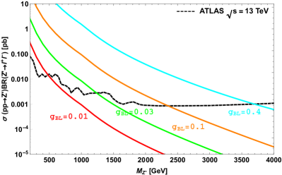
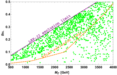
Figure 6: ATLAS dilepton constraints on the proposed model are shown. In the left panel, the black dashed line represents the exclusion limit from ATLAS [49], while the colored lines represent the dilepton signal cross sections for different values of $g_{BL}$ as a function of $M_{Z^{\prime}}$. The right panel shows ATLAS and LEP-II exclusion limits from dilepton searches in the plane of $M_{Z^{\prime}}-g_{BL}$.

6 Light neutrino mass

Field	$SU(2)_{L}\times U(1)_{Y}$	$U(1)_{B-L}$
$\eta$	$(\textbf{2},1/2)$	$-3$

Table 3: Inert doublet and its charge assignment.

Since the current model doesn’t contain the right-handed neutrinos, the standard type-I seesaw mechanism to generate light neutrino mass is not feasible with the existing particle content. However, the neutrino masses can be generated at one-loop level through radiative mechanism, which will be briefly described in this section. For this purpose, we Introduce an additional inert doublet $\eta=\begin{pmatrix}\eta^{+}\\ \frac{S+iA}{\sqrt{2}}\\ \end{pmatrix}$ with the $B-L$ charge $-3$. Thus, the trivial scalar potential gets modified with the inclusion of additional terms given as

$$V^{\prime} = V(H,\phi_{1},\phi_{8})+\mu_{\eta}(\eta^{\dagger}\eta)+\lambda_{\eta}(\eta^{\dagger}\eta)^{2}+\lambda^{\prime}_{H\eta}(H^{\dagger}\eta)(\eta^{\dagger}H)+\frac{\lambda_{\eta 18}}{2\Lambda^{3}}\left[(H^{\dagger}\eta)^{2}\phi_{8}\phi_{1}^{2}+{\rm h.c.}\right]$$ (6.1)

$$+ (\eta^{\dagger}\eta)\left[\lambda_{H\eta}(H^{\dagger}H)+\lambda_{\eta 1}(\phi_{1}^{\dagger}\phi_{1})+\lambda_{\eta 8}(\phi_{8}^{\dagger}\phi_{8})\right],$$

where $\Lambda$ is the cut-off parameter. The masses of real and imaginary components of the inert doublet $\eta$ are given as

$$M_{S}^{2} = \mu_{\eta}^{2}+\frac{\lambda_{\rm\eta 1}}{2}v^{2}_{1}+\frac{\lambda_{\eta 8}}{2}v^{2}_{8}+\left(\lambda_{H\eta}+\lambda^{\prime}_{H\eta}\right)\frac{v^{2}}{2}+\lambda_{\eta 18}\frac{v^{2}v_{1}^{2}v_{8}}{4\sqrt{2}\Lambda^{3}},$$

$$M_{A}^{2} = \mu_{\eta}^{2}+\frac{\lambda_{\rm\eta 1}}{2}v^{2}_{1}+\frac{\lambda_{\eta 8}}{2}v^{2}_{8}+\left(\lambda_{H\eta}+\lambda^{\prime}_{H\eta}\right)\frac{v^{2}}{2}-\lambda_{\eta 18}\frac{v^{2}v_{1}^{2}v_{8}}{4\sqrt{2}\Lambda^{3}}.$$ (6.2)

Figure 7: Radiative generation of neutrino mass

With these particle content, one can write the interaction term to generate light neutrino mass at one-loop level as shown in Fig. 7 as

$$\sum_{\alpha=1,2}Y_{i\alpha}\overline{(\ell_{L})}_{i}\tilde{\eta}N_{\alpha R}.$$ (6.3)

Thus, from Fig. 7, one can write the light neutrino mass matrix [53], as

$$({\cal M}_{\nu})_{ij}=\sum_{\alpha=1}^{2}{Y_{i\alpha}Y_{j\alpha}M_{D\alpha}\over 16\pi^{2}}\left[\frac{M_{S}^{2}}{M_{S}^{2}-M_{D\alpha}^{2}}\ln\frac{M_{S}^{2}}{M_{D\alpha}^{2}}-\frac{M_{A}^{2}}{M_{A}^{2}-M_{D\alpha}^{2}}\ln\frac{M_{A}^{2}}{M_{D\alpha}^{2}}\right].$$ (6.4)

Here $M_{D\alpha}=(U^{T}M_{R}U)_{\alpha}$ and $N_{D\alpha}=U^{\dagger}_{\alpha\beta}N_{\beta}$, with $M_{R}$ being the Majorana mass matrix. If we assume $m_{0}^{2}=(M^{2}_{S}+M^{2}_{A})/{2}$ is much greater than $M^{2}_{S}-M^{2}_{A}=\frac{\lambda_{\eta 18}}{2\sqrt{2}\Lambda^{3}}v^{2}v_{1}^{2}v_{8}$, the expression for the radiatively generated neutrino mass becomes

$$({\cal M}_{\nu})_{ij}={\lambda_{\eta 18}v^{2}v_{1}^{2}v_{8}\over 32\sqrt{2}\pi^{2}\Lambda^{3}}\sum_{\alpha=1}^{2}{Y_{i\alpha}Y_{j\alpha}M_{D\alpha}\over m_{0}^{2}-M_{D\alpha}^{2}}\left[1-{M_{D\alpha}^{2}\over m_{0}^{2}-M_{D\alpha}^{2}}\ln{m_{0}^{2}\over M_{D\alpha}^{2}}\right].$$ (6.5)

We further assume that inert doublet components are heavier than the DM mass. Note that for the parameter space considered here, the range of cutoff scale $\Lambda$, which is allowed by perturbative limits is $\sim[50,10^{4}]$ TeV. For example, with $(Y,\lambda_{\eta 18})\sim(10^{-1},10^{-2})$ and $(v_{1},v_{8},m_{0},M_{D\alpha},\Lambda)\sim(2,2,2,0.5,100)$ TeV, one can have $m_{\nu}\sim 10^{-11}$ GeV. Thus, the light neutrino mass generation can be successfully achieved in the proposed model.

7 Conclusion

In this article, we made a detailed study of Majorana dark matter in a variant of $B-L$ model where the gauge symmetry is extended with a $U(1)_{B-L}$. The current model is enriched with three exotic fermions with $B-L$ charges $-4,-4,+5$, to avoid the triangle gauge anomalies. The scalar sector is equipped with two additional scalar singlets $\phi_{1}$ and $\phi_{8}$ with $B-L$ charges $-1,+8$ to break the $U(1)_{B-L}$ gauge symmetry giving mass to the exotic fermions and the heavy gauge boson $Z^{\prime}$. The structure of the model is extremely fruitful, giving two kinds of mediators that connect the visible and dark sectors. The lightest mass eigenstate upon the diagonalization of exotic fermion mass matrix, plays the role of dark matter. The scalar portal relic abundance has been studied with all possible annihilation channels and the effect of massless physical Goldstone boson is suitably addressed. The SI cross section has been calculated and investigated with the current limits from LUX (2016), XENON1T (2017) and PandaX (2017). Similar strategy is repeated for $Z^{\prime}$-portal channels. But in the $Z^{\prime}$ case, it is not possible to study for direct searches as the Majorana dark matter couples axial-vectorially with the $Z^{\prime}$, while SM quarks couple to $Z^{\prime}$ vectorially. In collider searches, the ATLAS bounds on the $Z^{\prime}$ mass and $g_{BL}$ impose strong constraints. However, we still have a viable parameter space satisfying the current relic density and the dilepton bounds. We have also addressed the generation of light neutrino mass by adding an additional inert doublet $\eta$ with $B-L$ charge assigned as $-3$. To conclude, we have made a complete systematic study of Majorana dark matter in a new variant of $B-L$ gauge extended model. This simple model survives the current collider limits while satisfies dark matter constraints and can be probed in future high luminosity data from LHC.

References

- [1] Planck, P. A. R. Ade et al., “Planck 2015 results. XIII. Cosmological parameters,” Astron. Astrophys. 594 (2016) A13, arXiv:1502.01589.
- [2] F. Zwicky, “On the Masses of Nebulae and of Clusters of Nebulae,” Astrophys. J. 86 (1937) 217–246.
- [3] V. C. Rubin and W. K. Ford, Jr., “Rotation of the Andromeda Nebula from a Spectroscopic Survey of Emission Regions,” Astrophys. J. 159 (1970) 379–403.
- [4] D. Clowe, A. Gonzalez, and M. Markevitch, “Weak lensing mass reconstruction of the interacting cluster 1E0657-558: Direct evidence for the existence of dark matter,” Astrophys. J. 604 (2004) 596–603, arXiv:astro-ph/0312273.
- [5] E. E. Jenkins, “Searching for a () Gauge Boson in Collisions,” Phys. Lett. B192 (1987) 219–222.
- [6] W. Buchmuller, C. Greub, and P. Minkowski, “Neutrino masses, neutral vector bosons and the scale of B-L breaking,” Phys. Lett. B267 (1991) 395–399.
- [7] L. Basso, A. Belyaev, S. Moretti, and C. H. Shepherd-Themistocleous, “Phenomenology of the minimal B-L extension of the Standard model: Z’ and neutrinos,” Phys. Rev. D80 (2009) 055030, arXiv:0812.4313.
- [8] W. Emam and S. Khalil, “Higgs and Z-prime phenomenology in B-L extension of the standard model at LHC,” Eur. Phys. J. C52 (2007) 625–633, arXiv:0704.1395.
- [9] S. Khalil, “Low scale - L extension of the Standard Model at the LHC,” J. Phys. G35 (2008) 055001, arXiv:hep-ph/0611205.
- [10] S. Iso, N. Okada, and Y. Orikasa, “Classically conformal extended Standard Model,” Phys. Lett. B676 (2009) 81–87, arXiv:0902.4050.
- [11] S. Kanemura, T. Matsui, and H. Sugiyama, “Neutrino mass and dark matter from gauged breaking,” Phys. Rev. D90 (2014) 013001, arXiv:1405.1935.
- [12] M. Lindner, D. Schmidt, and T. Schwetz, “Dark Matter and neutrino masses from global U(1)B−L symmetry breaking,” Phys. Lett. B705 (2011) 324–330, arXiv:1105.4626.
- [13] N. Okada and S. Okada, “ portal dark matter and LHC Run-2 results,” Phys. Rev. D93 (2016) no. 7, 075003, arXiv:1601.07526.
- [14] N. Okada and S. Okada, “-portal right-handed neutrino dark matter in the minimal U(1)X extended Standard Model,” Phys. Rev. D95 (2017) no. 3, 035025, arXiv:1611.02672.
- [15] S. Bhattacharya, S. Jana, and S. Nandi, “Neutrino Masses and Scalar Singlet Dark Matter,” Phys. Rev. D95 (2017) no. 5, 055003, arXiv:1609.03274.
- [16] A. Biswas, S. Choubey, and S. Khan, “Galactic gamma ray excess and dark matter phenomenology in a model,” JHEP 08 (2016) 114, arXiv:1604.06566.
- [17] W. Wang and Z.-L. Han, “Radiative linear seesaw model, dark matter, and ,” Phys. Rev. D92 (2015) 095001, arXiv:1508.00706.
- [18] T. Basak and T. Mondal, “Constraining Minimal model from Dark Matter Observations,” Phys. Rev. D89 (2014) 063527, arXiv:1308.0023.
- [19] P. Bandyopadhyay, E. J. Chun, and R. Mandal, “Implications of right-handed neutrinos in extended standard model with scalar dark matter,” arXiv:1707.00874.
- [20] V. De Romeri, E. Fernandez-Martinez, J. Gehrlein, P. A. N. Machado, and V. Niro, “Dark Matter and the elusive in a dynamical Inverse Seesaw scenario,” arXiv:1707.08606.
- [21] N. Okada and O. Seto, “Higgs portal dark matter in the minimal gauged model,” Phys. Rev. D82 (2010) 023507, arXiv:1002.2525.
- [22] S. Kanemura, O. Seto, and T. Shimomura, “Masses of dark matter and neutrino from TeV scale spontaneous breaking,” Phys. Rev. D84 (2011) 016004, arXiv:1101.5713.
- [23] O. Seto and T. Shimomura, “Atomki anomaly and dark matter in a radiative seesaw model with gauged symmetry,” Phys. Rev. D95 (2017) no. 9, 095032, arXiv:1610.08112.
- [24] E. Ma and R. Srivastava, “Dirac or inverse seesaw neutrino masses with gauge symmetry and flavor symmetry,” Phys. Lett. B741 (2015) 217–222, arXiv:1411.5042.
- [25] E. Ma and R. Srivastava, “Dirac or inverse seesaw neutrino masses from gauged symmetry,” Mod. Phys. Lett. A30 (2015) no. 26, 1530020, arXiv:1504.00111.
- [26] E. Ma, N. Pollard, R. Srivastava, and M. Zakeri, “Gauge Model with Residual Symmetry,” Phys. Lett. B750 (2015) 135–138, arXiv:1507.03943.
- [27] S. Patra, W. Rodejohann, and C. E. Yaguna, “A new B-L model without right-handed neutrinos,” JHEP 09 (2016) 076, arXiv:1607.04029.
- [28] J. C. Montero and V. Pleitez, “Gauging U(1) symmetries and the number of right-handed neutrinos,” Phys. Lett. B675 (2009) 64–68, arXiv:0706.0473.
- [29] D. Nanda and D. Borah, “Common origin of neutrino mass and dark matter from anomaly cancellation requirements of a model,” Phys. Rev. D96 (2017) no. 11, 115014, arXiv:1709.08417.
- [30] S. Singirala, R. Mohanta, and S. Patra, “Singlet scalar Dark matter in models without right-handed neutrinos,” arXiv:1704.01107.
- [31] J. Erler, P. Langacker, S. Munir, and E. Rojas, “Improved Constraints on Z-prime Bosons from Electroweak Precision Data,” JHEP 08 (2009) 017, arXiv:0906.2435.
- [32] G. Belanger, B. Dumont, U. Ellwanger, J. F. Gunion, and S. Kraml, “Status of invisible Higgs decays,” Phys. Lett. B723 (2013) 340–347, arXiv:1302.5694.
- [33] P. P. Giardino, K. Kannike, I. Masina, M. Raidal, and A. Strumia, “The universal Higgs fit,” JHEP 05 (2014) 046, arXiv:1303.3570.
- [34] S. Weinberg, “Goldstone Bosons as Fractional Cosmic Neutrinos,” Phys. Rev. Lett. 110 (2013) no. 24, 241301, arXiv:1305.1971.
- [35] C. Garcia-Cely, A. Ibarra, and E. Molinaro, “Dark matter production from Goldstone boson interactions and implications for direct searches and dark radiation,” JCAP 1311 (2013) 061, arXiv:1310.6256.
- [36] Planck, P. A. R. Ade et al., “Planck 2013 results. XVI. Cosmological parameters,” Astron. Astrophys. 571 (2014) A16, arXiv:1303.5076.
- [37] A. V. Semenov, “LanHEP: A Package for automatic generation of Feynman rules in gauge models,” arXiv:hep-ph/9608488.
- [38] A. Pukhov, E. Boos, M. Dubinin, V. Edneral, V. Ilyin, D. Kovalenko, A. Kryukov, V. Savrin, S. Shichanin, and A. Semenov, “CompHEP: A Package for evaluation of Feynman diagrams and integration over multiparticle phase space,” arXiv:hep-ph/9908288.
- [39] G. Belanger, F. Boudjema, A. Pukhov, and A. Semenov, “MicrOMEGAs 2.0: A Program to calculate the relic density of dark matter in a generic model,” Comput. Phys. Commun. 176 (2007) 367–382, arXiv:hep-ph/0607059.
- [40] G. Belanger, F. Boudjema, A. Pukhov, and A. Semenov, “Dark matter direct detection rate in a generic model with micrOMEGAs 2.2,” Comput. Phys. Commun. 180 (2009) 747–767, arXiv:0803.2360.
- [41] DELPHI, OPAL, LEP Electroweak, ALEPH, L3, S. Schael et al., “Electroweak Measurements in Electron-Positron Collisions at W-Boson-Pair Energies at LEP,” Phys. Rept. 532 (2013) 119–244, arXiv:1302.3415.
- [42] P. Agrawal, Z. Chacko, C. Kilic, and R. K. Mishra, “A Classification of Dark Matter Candidates with Primarily Spin-Dependent Interactions with Matter,” arXiv:1003.1912.
- [43] J.-M. Zheng, Z.-H. Yu, J.-W. Shao, X.-J. Bi, Z. Li, and H.-H. Zhang, “Constraining the interaction strength between dark matter and visible matter: I. fermionic dark matter,” Nucl. Phys. B854 (2012) 350–374, arXiv:1012.2022.
- [44] N. Okada and Y. Orikasa, “Dark matter in the classically conformal B-L model,” Phys. Rev. D85 (2012) 115006, arXiv:1202.1405.
- [45] J. R. Ellis, A. Ferstl, and K. A. Olive, “Reevaluation of the elastic scattering of supersymmetric dark matter,” Phys. Lett. B481 (2000) 304–314, arXiv:hep-ph/0001005.
- [46] LUX, D. S. Akerib et al., “Results from a search for dark matter in the complete LUX exposure,” Phys. Rev. Lett. 118 (2017) no. 2, 021303, arXiv:1608.07648.
- [47] XENON, E. Aprile et al., “First Dark Matter Search Results from the XENON1T Experiment,” arXiv:1705.06655.
- [48] PandaX-II, X. Cui et al., “Dark Matter Results From 54-Ton-Day Exposure of PandaX-II Experiment,” Phys. Rev. Lett. 119 (2017) no. 18, 181302, arXiv:1708.06917.
- [49] “Search for new phenomena in the dilepton final state using proton-proton collisions at √ s = 13 TeV with the ATLAS detector,” Tech. Rep. ATLAS-CONF-2015-070, CERN, Geneva, Dec, 2015. https://cds.cern.ch/record/2114842.
- [50] A. Belyaev, N. D. Christensen, and A. Pukhov, “CalcHEP 3.4 for collider physics within and beyond the Standard Model,” Comput. Phys. Commun. 184 (2013) 1729–1769, arXiv:1207.6082.
- [51] K. Kong, “TASI 2011: CalcHEP and PYTHIA Tutorials,” in The Dark Secrets of the Terascale: Proceedings, TASI 2011, Boulder, Colorado, USA, Jun 6 - Jul 11, 2011, pp. 161–198. 2013. arXiv:1208.0035. https://inspirehep.net/record/1124593/files/arXiv:1208.0035.pdf.
- [52] M. Klasen, F. Lyonnet, and F. S. Queiroz, “NLO+NLL Collider Bounds, Dirac Fermion and Scalar Dark Matter in the B-L Model,” arXiv:1607.06468.
- [53] E. Ma, “Verifiable radiative seesaw mechanism of neutrino mass and dark matter,” Phys. Rev. D73 (2006) 077301, arXiv:hep-ph/0601225.