Exact Ground States of the Kaya-Berker Model

Abstract

Here we study the two-dimensional Kaya-Berker model, with a site occupancy $p$ of one sublattice, by using a polynomial-time exact ground-state algorithm. Thus, we were able to obtain $T=0$ results in exact equilibrium for rather large system sizes up to $777^{2}$ lattice sites. We obtained sublattice magnetization and the corresponding Binder parameter. We found a critical point $p_{c}=0.6423(3)$ beyond which the sublattice magnetization vanishes. This is clearly smaller than previous results which were obtained by using non-exact approaches for much smaller systems. We also created for each realization minimum-energy domain walls from two ground-state calculations for periodic and anti-periodic boundary conditions, respectively. The analysis of the mean and the variance of the domain-wall distribution shows that there is no thermodynamic stable spin-glass phase, in contrast to previous claims about this model.

I Introduction

Compared to regular or pure systems, magnetic systems with quenched disorder, like spin glasses and random-field systems Young (1997), exhibit many peculiar properties. Their complex low-temperature behavior is still not fully understood, even for two-dimensional systems. As analytical solutions are not available, computer simulation studies Hartmann (2015) are often performed. With respect to Markov-chain Monte Carlo simulations Newman and Barkema (1999), one of the difficulty is their slow glassy dynamic, resulting in very long equilibration times. Other approaches to study spin-glasses involve finding and characterizing ground states Hartmann and Rieger (2001, 2004). In three or more dimensions, only algorithms with exponential running time are known, but in two dimensions polynomial time algorithms are available. One of the interesting differences between 2D and 3D spin-glasses is that so far all 2D models with short or finite-range interactions show a transition temperature $T_{\text{c}}=0$ McMillan (1984); Bray and Moore (1984); Saul and Kardar (1993); Rieger et al. (1996); Houdayer (2001); Hartmann and Young (2001); Carter et al. (2002); Hartmann (2003). At all finite temperatures the spin-glass phase vanishes for 2D models. In contrast the 3D models show a transition temperature above zero. This spawned the search for 2D models with a finite critical temperature. One such candidate is the Kaya-Berker model Kaya and Berker (2000), which was claimed to exhibit a spin-glass like phase for non-zero temperatures, i.e., a phase transition at a finite temperature. This previous claim was based on numerical studies of rather small systems with non-exact algorithms. Here, we will present results for this model which we obtained by using exact and fast ground-state algorithms. This allowed us to study in exact equilibrium rather large systems exhibiting more than $10^{5}$ spins. Our result strongly suggest that in contrast to previous claims, the model does not exhibit an ordered low-temperature phase.

The manuscript is organized as follows: We will first introduce the model along with suitable measurable quantities and review previous results. Next, we outline the algorithm we have used to obtain exact ground states, and, by changing the boundary conditions, to obtain domain-wall (DW) energies. In the main part, we will present our results, followed by our conclusions.

II Model

The Kaya-Berker Model Kaya and Berker (2000) is a variation of the Ising model on a two-dimensional triangular lattice with $N=L_{x}\times L_{y}$ spins. The spins $s_{i}$ take the values $\pm 1$ and all bonds are antiferromagnetic. It’s Hamiltonian is given by

$$\mathcal{H}=-J\sum_{\langle i,j\rangle}\epsilon_{i}s_{i}\epsilon_{j}s_{j}\,,$$ (1)

with $J<0$ and $\langle i,j\rangle$ indicating a sum over all nearest-neighbor pairs. The model allows for dilution, which is described by the quenched disorder variables $\epsilon_{i}\in\{0,1\}$. Every spin is located on one of three sublattices, such that every spin has only neighbors in the two other sublattices. Fig. 1 shows the triangular lattice and subdivision into three sublattices. Here, one of the sublattices is diluted and only a fraction $p$ of spin sites is occupied ($\epsilon_{i}=1$), while a fraction $1-p$ of sites is not occupied by a spin ($\epsilon_{i}=0$).

Figure 1: (Color online) $6\times 4$ triangular lattice showing the subdivision into the three sublattices, as indicated by the three colors of the nodes (white, gray, black). Every triangle is frustrated, since not all bonds can be satisfied.

In the fully occupied $p=1$ case, every triangle of spins is frustrated. This special configuration was solved exactly Wannier (1950); Houtappel (1950), with the result that the system is disordered at all temperatures. Ground states are characterized by exactly one-third of unsatisfied bonds. While there are some configurations that are ordered, e.g., alternating row of all up-spins with row of all down-spins, no energy advantage is obtained for long-range order. Because of entropic dominance, i.e., the exponential dominance of these non-ordered ground state configurations, no long-range order occurs

For the diluted $p=0$ case, one obtains a honeycomb lattice, where the frustration is fully relieved. The ground state is ordered and spins are aligned antiparallel with all of their neighbors. Within the two remaining sublattices spins in the same sublattices are aligned in the same direction.

By choosing an intermediate value of $p$, the number of frustrated plaquettes can be varied. The behavior of the system is complicated and allows for interesting behavior. These intermediate values of $p$ result in a ground state with zero magnetization on the diluted lattice and roughly equal but opposite magnetization on the two undiluted lattices. The order parameter is therefore defined as the per-lattice magnetization

$$m_{\alpha}=\frac{1}{N_{\alpha}}\sum_{i\in\alpha}\epsilon_{i}s_{i}\,,$$ (2)

with $\alpha=a,b,c$ denoting one of the three sublattices and $N_{\alpha}=\sum_{i\in\alpha}\epsilon_{i}$ is the number of spins of sublattice $\alpha$. The diluted lattice will be lattice $a$.

A model similar to the Kaya-Berker model with uniform dilution in all sublattices Grest and Gabl (1979); Blackman et al. (1981); Andérico et al. (1982); Tang et al. (2010) was studied earlier. While the first study observed spin-glass behavior, all later publications argue against a spin-glass phase. However, they found a large but finite correlation between spins, which could be mistaken for long-range order in small systems. In 2000 H. Kaya and A. N. Berker devised the aforementioned model, which notably differs from the older model by restricting the dilution to one sublattice Kaya and Berker (2000). The authors studied it using hard-spin mean field (HSMF) theory. For HSMF, each spin $s_{i}$ does not only interact with its neighbours $s_{j}$ through their mean spin values $m_{j}$ as in standard mean-field theory. Instead, the self-consistent equation for the site-dependent mean values $m_{j}$ involves a sum over all possible $2^{n}$ configurations of the $n$ neighbours such that each spin orientation $s_{j}=\pm 1$ occurs with a probability which is compatible with its mean value $m_{j}$. As a further approximation, in Ref. Kaya and Berker (2000) the disorder average is performed and the site dependent mean values are replaced by their sublattice mean values, resulting in three coupled equations. For the sublattice spin-glass order parameter (which involves again the site-dependent mean values)

$$q_{\alpha}=\left[\frac{1}{N_{\alpha}}\sum_{i\in\alpha}(m_{i}-m_{\alpha})^{2}\right]^{1/2}\,,$$ (3)

they found nonzero values at finite temperatures for occupancy $p<0.958$. However, their study involves only small system with sizes up to $30\times 30$ and features no finite-size scaling analysis. Other studies analyzed the Kaya-Berker model using Monte Carlo (MC) simulations Robinson (2003); Robinson et al. (2011), effective-field theory (EFT) Žukovič et al. (2012) and a modified pair-approximation (PA) method Balcerzak et al. (2014). The EFT approach is based on a cluster approximation with clusters comprised of only a single spin and interactions with their nearest neighbors Žukovič et al. (2010), which is quite similar to HSMF. The PA method is based on the cumulant expansion of the entropy. So far, none of the studies found conclusive evidence in favor or against the spin-glass phase at finite temperatures. Note that using MC simulations the system certainly appears to behave like a glassy system in the accessible system sizes and timescales. Here simulations at different and large enough system sizes and proof of proper equilibration would be needed, which is difficult and requires a huge numerical effort for glassy systems.

This work aims to settle this open question by using an exact ground state algorithm which allowed us to investigate large systems in equilibrium. Studying exact ground states allows calculating domain wall energies, which are often used Bray and Moore (1984); McMillan (1984); Hartmann (1999); Hartmann and Young (2001); Amoruso et al. (2003); Romá et al. (2007) to verify the stability of a phase at finite temperatures. In the following section we explain our numerical approaches.

III Algorithm

The ground state algorithm is taken from Ref. Melchert and Hartmann (2011) where it’s used to calculate ground states of the 2D random bond Ising model on a planar triangular lattice. Here we present only a short summary of the algorithm, visualized in Fig. 2.

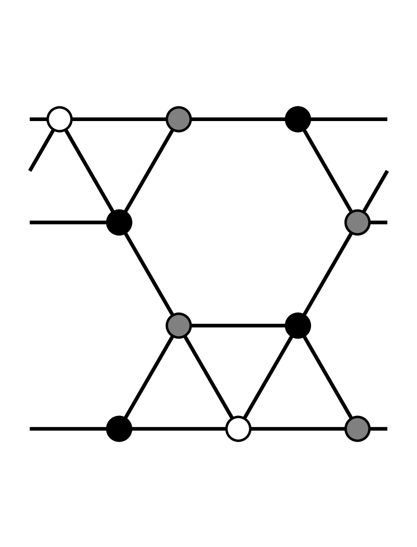
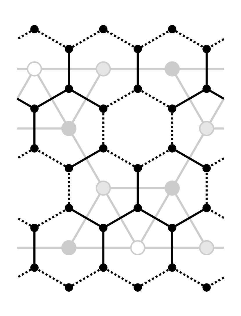
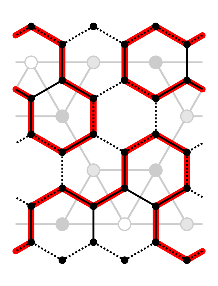
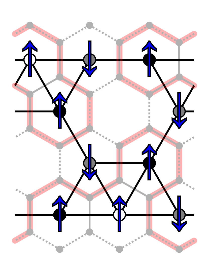
Figure 2: (Color online) Illustration of the steps involved in the ground state calculation. The sample shows a $3\times 4$ system with periodic boundary conditions in the horizontal direction. (a) Initial system with $p=0.5$ occupation on the white sublattice. (b) Construction of the dual graph of the original undiluted system with additional vertices and edges at the top and bottom. Edges that do not correspond to edges in the diluted system carry zero weight and are marked using stroked lines. (c) Set of minimal weighted loops on the dual graph. These paths separate clusters of aligned spins. (d) Ground state constructed by setting the top left spin to up and assigning all remaining spins using the clusters determined earlier.

We start with a specific realization of our system, that we want to calculate a GS for. Lattice sites and bonds are interpreted as the nodes and edges of a a weighted undirected graph $G$. The weights are given by the strength of the bonds. For this example, all weights are set to $-1$, but the algorithm is suitable for arbitrary weights. Here we consider periodic boundary conditions in horizontal ($x$) direction and open boundary conditions in vertical direction.

Next, we construct an auxiliary graph $G^{\prime}$, which is the dual graph of the undiluted triangular lattice, but with two additional rows of each $2L_{x}$ vertices at the top and bottom, respectively. The resulting graph contains a total of $(2L_{x})\times(L_{y}+1)$ vertices and has the structure of a honeycomb lattice. Since the $2L_{x}\times(L_{y}-1)$ faces in $G$ are separated by single edges, there is a corresponding dual edge in $G^{\prime}$ for every edge in $G$. Each dual edge basically “crosses” the corresponding edge from $G$. These edges carry the same weight as the corresponding edges in $G$. Note that the dilution is modelled by making the bonds site dependent $J\,\to\,J_{i,j}\in\{0,J\}$ and setting the weight to zero of edges which are adjacent to non-occupied sites. Also the additional edges in $G^{\prime}$, i.e., all the edges at the top and bottom which do not correspond to an edge in $G$, are assigned zero weight.

In the next step, a set of closed non-intersecting loops with minimum edge weight are calculated. Calculating this set is part of the negative-weight percolation Melchert and Hartmann (2008) problem, which yields a globally optimal solution. This works by transforming the problem into a minimum-weight perfect matching problem which is a standard problem in graph theory and can be solved exactly in a time growing only polynomially with system size. Note that while the total edge weight of the whole set of loops is optimized, each individual loop has a total negative or zero weight. These loops separate clusters of aligned spins that form a GS of the system. Suppose two spins share a bond that favors antiparallel alignment, then the corresponding edge in $G^{\prime}$ that separates these spins carries a negative weight. Because we look for minimal weighted loops, this edge is likely to be included in one of the loops and thus the spins are in different clusters, fulfilling the antiparallel alignment of the bond. In general, the weight of a loop is the negative of the energy of the DW surrounding the spins inside the loop. Therefore, by flipping the spins inside a loop, the total energy will be decreased by twice this amount.

Therefore, the last step is to construct a ground state from the minimal weighed loops. This is achieved by arbitrarily setting the top left spin to up. The orientation of neighboring spins can then be determined by looking at the loops. If spins are separated by a loop they need be aligned in opposite direction. This process is repeated until all spin have been assigned an orientation. Since there is no external field, the configuration obtained by a global spin flip is also a GS of the system.

From the calculated GS, we can easily obtain the magnetization values of the sublattices. Nevertheless, due to the discrete structure of the model, the GS is highly degenerate. Therefore, we used a small randomization of the bonds to lift the degeneracy. Instead of the original bonds values $J_{i,j}=0,-1$, we used

$$\hat{J}_{i,j}=S\,J_{i,j}+X_{i,j}\,,$$ (4)

with a constant scaling factor $S$ and uniform distributed discrete random variables $X_{i,j}\in\{-V,-V+1,\ldots,V-1,V\}\subset\mathbb{Z}$. The values $S=10^{6}$ and $V=100$ are used throughout the remaining analysis. The large scaling factor is used to keep the bond strength an integer, while allowing for slight variations such that the ground state of the modified system is also a GS of the original system, for each realization. Although this randomization does not guarantee a uniform sampling of the ground states, it was shown Amoruso and Hartmann (2004) that for the two-dimensional random-bond Ising model, the influence of the bias is very weak such that the results are reliable within the statistical error bars.

Furthermore, we also studied the scaling of domain-wall energies. The DWs are induced McMillan (1984); Bray and Moore (1984); Saul and Kardar (1993); Rieger et al. (1996); Hartmann and Young (2001) for a given realization by first calculating the GS for the original system, leading to a ground state energy $E_{p}$. Another GS is obtained for a modified system such that a domain wall is induced. Here, the second GS with energy $E_{ap}$ is calculated for a system, where the boundary conditions are switched from periodic to antiperiodic in the horizontal direction. The switch of the boundary conditions is realized by inverting the sign of the bonds in one (top-bottom) column of bonds. The changed boundary conditions induce that in the GS the spins left and right of the switched bonds obtain relative orientations opposite to the ground states. Due to the periodicity in the horizontal direction, there must be another line where the relative orientation of the spins across the line is opposite to the relative orientation in the GS of the original system. This is the domain wall generated by this procedure. The energy of the domain wall is given by

$$\Delta E=E_{\rm p}-E_{\rm ap}\,.$$ (5)

If the disorder-averaged value $\langle\Delta E\rangle$ increases with system size, domain walls become more and more expensive, thus an ordered state with nonzero order parameter $m_{\alpha}$ is stable. On the other hand, if $\langle\Delta E\rangle$ decreases with system size, for large systems arbitrary small thermal fluctuations will be sufficient to destroy an ordered state, which means $T_{\text{c}}=0$. Nevertheless, a non-magnetized state might exhibit spin-glass order. This is signified by a growth of the width $\sigma(\Delta E)$ of the (disorder) distribution of domain-wall energies when increasing the system size $L$, while the average $\langle\Delta E\rangle$ decreases. Equivalently to the width, one could monitor the size dependence of the average $\langle|\Delta E|\rangle$ of the absolute value of the domain-wall energy. Below, we will use this approach to show that the KS model exhibits indeed a global antiferromagnetic order, i.e., a ferromagnetic order for the fully occupied sublattices, for certain values of $p$, but no spin glass order.

IV Results

To obtain the following results, between 5000 and 10000 random realizations of the disorder for the Kaya-Berker model were studied for various system sizes, for many values of the disorder parameter $p$. We studied square systems $L=L_{x}=L_{y}$ with $L\in[30,345]$. For each realization we calculated exact ground states of the system with periodic and anti-periodic boundary conditions, respectively. Each realization and both GSs are saved to disk and are analyzed later. All systems have open boundary conditions in the $y$-direction, since the GS algorithm cannot handle periodicity in both directions. This does not impact the ordering of the system, as the change of boundary conditions, to induce a domain wall, is performed perpendicular to the open boundary condition. The DW therefore spans the system between the open boundaries.

First the magnetization of the Kaya-Berker model in the ground state is studied. The magnetization (2) is calculated per lattice and plotted as a function of the fraction of occupied spins $p$. The sign of the sublattice magnetization is chosen so that magnetization for lattice $b$ is always positive. One problem with calculating GSs is that most observables depend on the specific GS that is generated. The discrete nature of the Kaya-Berker model results in exponentially many GSs, all sharing the same energy, but varying in other properties. This could lead to biased results if the GS algorithm favors specific states. In fact this is the case for the presented GS algorithm, as visible in Fig. 3, where we compare the resulting magnetizations for the original bonds and for bonds slightly randomized according to Eq. (4).

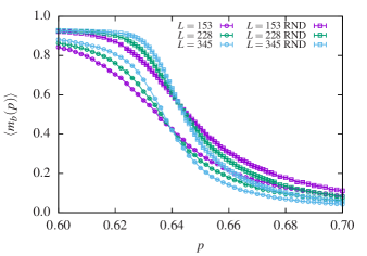
Figure 3: (Color online) Magnetization of sublattice $b$ at different fractions $p$ of occupied sites and system sizes $L$. The RND data sets include slight variations of the bond strengths according to Eq. (4).

All the magnetization values without bond randomization are clearly lower than the ones with randomization. The intersection of the curves also shifts slightly to the right when bond randomization is used. As mentioned above, our final results are obtained for the slightly randomized realizations.

Next, the critical point is determined by performing a finite-size scaling analysis of the Binder parameter Binder (1981)

$$b_{\alpha}=\frac{1}{2}\left(3-\frac{\langle m_{\alpha}^{4}\rangle}{\langle m_{\alpha}^{2}\rangle^{2}}\right)$$ (6)

for the data of the slightly randomized systems. When plotting $b$ as a function of the disorder parameter $p$, the curves for different system sizes $L$ will intersect (for large enough system sizes) at the critical point $p_{c}$ where the sub lattice ferromagnetic (global antiferromagnetic) order disappears. This allows for a convenient determination of the critical point. Furthermore, finite-size scaling Cardy (1988) shows that when rescaling the $p$ axis according to $(p-p_{c})L^{1/\nu}$, for the correct value of $p_{c}$ and a suitably chosen value of $\nu$, the data will collapse onto a single curve. More precisely, the Binder parameter follows

$$b(p,L)=\tilde{b}\left((p-p_{c})L^{1/\nu}\right)\,,$$ (7)

where $\tilde{b}(\ldots)$ is a non-size-dependent function of one scaled variable. The quantity $\nu$ is a critical exponent which describes the divergence of the correlation length when approaching a second-order phase transition. The actual value of $\nu$ (together with other critical exponents) allows to classify second-order phase transitions according to universality classes.

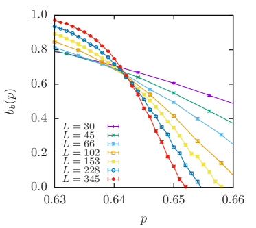
Figure 4: (Color online) Binder parameter of sublattice $b$ as a function of the sublattice occupancy $p$, for different system sizes.

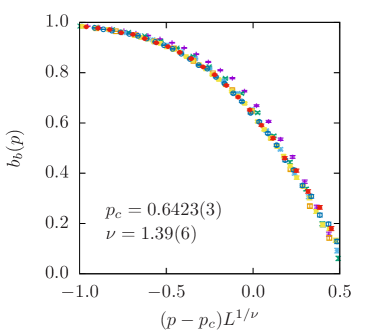
Figure 5: (Color online) Rescaled Binder parameter with a rescaled $p$-axis using the appropriate scaling variables $p_{c}=0.6423(3)$, $\nu=1.39$.

The results for the Binder parameter and the best data collapse, as obtained from the autoscale script Melchert (2009) are shown in Figs. 4 and 5. The $x$-range of the collapse was restricted to $[-0.75,0.25]$, which gave the best collapse quality of $S=1.17$. $S$ describes the mean-squared fluctuation of the data along the collapse curve measured in autoscale in terms of error bars. The system sizes $L=30$ and $L=45$ were excluded from the data collapse, since they deviate from the other curves and resulted in a worse collapse. This is because of their quite small system size, which would require additional corrections to match the other curves. We find that the Kaya-Berker model has a critical point of $p_{\text{c}}=0.6423(3)$. This result is much smaller than any of the previous results of $p_{\text{c}}=0.958$ by Kaya and Berker Kaya and Berker (2000), $p_{\text{c}}\approx 0.95$ by using a Monte Carlo simulation Robinson (2003), or $p_{\text{c}}=0.875$ obtained using effective-field theory (EFT) Žukovič et al. (2012). However, the discrepancy can be explained by taking a closer look at the previously used methods. First, the results by Kaya and Berker are obtained by HSMF theory. This method includes several approximations, like the mean-field nature of the approach and the partial use of locally averaged magnetizations. Furthermore, this method includes a form of stochastic iterations. These iterations often gets stuck in local minima. In fact, the authors found a multiplicity of solutions and used only the most stable set to determine the critical point. Other not so stable solutions are fragmented and show a much lower magnetization than the stable one. Indeed the solution with the lowest magnetization looks like it could become zero somewhere around $0.6<p<0.7$, which would coincide with our $p_{\text{c}}=0.6423(3)$ result. The other result obtained by MC simulations also suffers from the problem that the dynamic of the Kaya-Berker model becomes very slow at low temperatures and often also gets stuck in local energy minima. Last, the other approaches, which are very similar to the further approximation of HSMF, impose also sublattice-wise uniformity of the magnetization. This restriction may not capture the whole behavior of the model, leading to wrong results. Therefore, the exact GS approach which we used here is much more reliable than any of the previous results since it neither includes approximations nor it does suffer from convergence problems. Finally, we can treat much larger sizes compared to the previous approaches.

Although we are here not mainly interested in characterizing the phase transition, we also obtained an estimate $\nu=1.39(6)$ for the value of the critical exponent of the correlation length. No corresponding result for the Kaya-Berker model for this critical exponent at the antiferromagnet-paramagnet transition is known to us in the literature. Thus a direct comparison is not possible. Nevertheless, for the random-bond Ising model, which exhibits a ferromagnet-paramagnet transition (with spin-glass behavior at exactly $T=0$), a value $\nu=1.55(1)$ was found Amoruso and Hartmann (2004). This is not fully compatible, but only two error bars away from the value obtained here. Therefore, the transitions might be in the same universality class. Anyway, we proceed towards our main aim of the paper, to show that no thermodynamic stable spin-glass phase exists.

Next, the domain wall length $l$ is studied. This is another property which strongly depends on the specific GS of a given realization. As explained above, DWs are obtained by calculating the GS of a realization, flipping the boundary condition, calculating a new GS, and comparing the two obtained GS. Note that the bond randomization is again used, which should result in typical domain wall lengths among many possible degenerate DWs. This is sufficient for the present purpose of identifying the transition point where the order disappears. A more sophisticated method to determine shortest and maximal length domain walls is presented in Ref. Melchert and Hartmann (2007). This analysis uses $10,000$ samples for each system size $L\in[30,777]$ and occupancy value $p$. Some exemplary domain walls at different occupancy $p$ are shown in Fig. 6. For small values of $p$, where the GS is ordered, the DWs are very straight. With increasing value of $p$ the domain walls become more fractal.

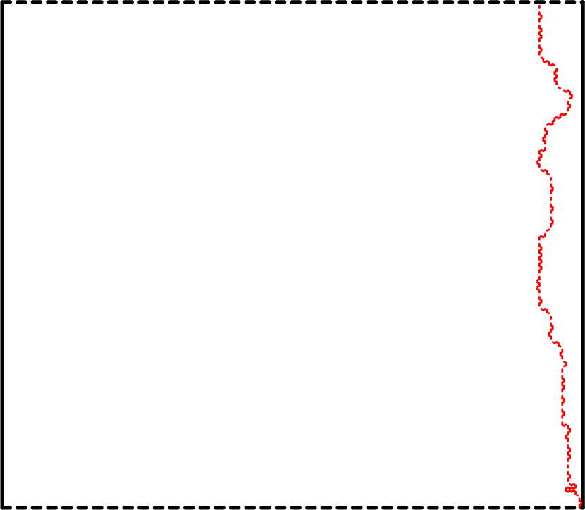
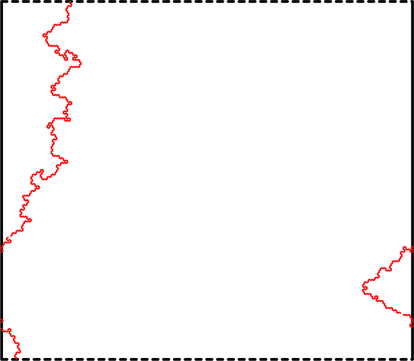
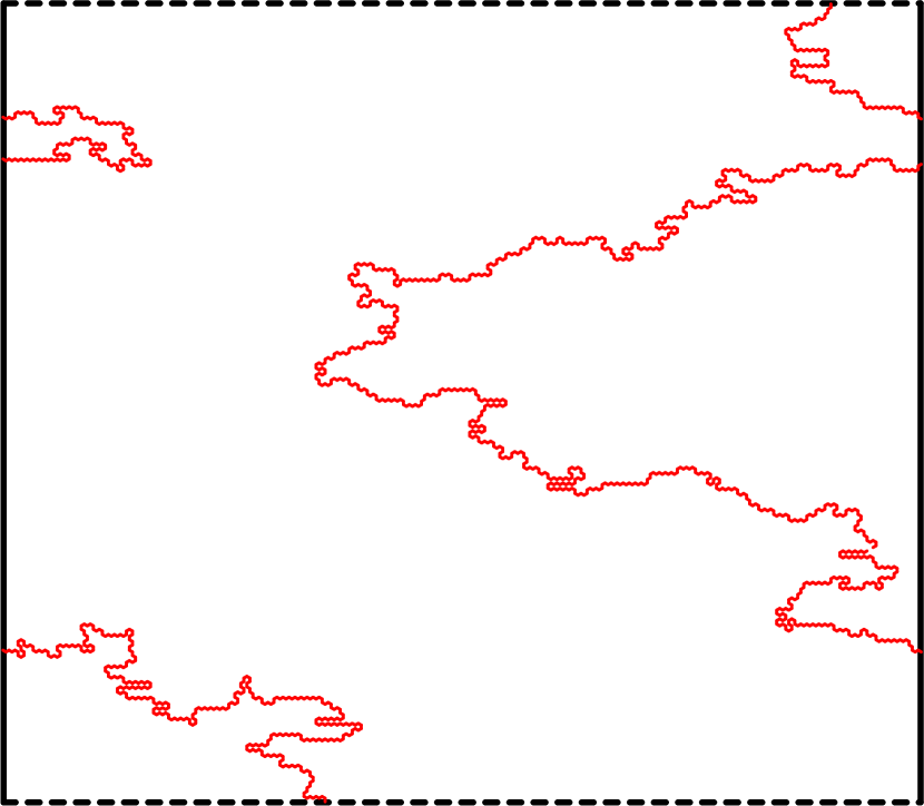
Figure 6: (Color online) Exemplary domain walls at different occupancy. The solid and dashed border marks periodic and open boundary conditions respectively. The occupancy was set to $p=0.2$ (left), $p=0.6$ (center) and $p=0.8$ (right).

The measured averaged lengths $l$ of the DWs are shown in Fig. 7 as a function of the system size $L$. All of the data sets show a clean power-law behavior of the form

$$l(L)\sim L^{d_{\rm f}}\,.$$ (8)

where $d_{f}$ is the fractal exponent which depends on $p$. A power-law fit was performed for all data sets, excluding the small system sizes $L<50$. The fits match the data sets very well. The resulting fractal dimension $d_{\text{f}}$, see Fig. 8, exhibits a change between the $p\leq 0.65$ and $p\geq 0.70$ data sets visible as a rather sharp jump in the plot. Apart from this sharp jump, the fractal dimension also grows slowly with the occupancy. By interpolating between the two values closest to the critical point at $p=0.64$ and $p=0.645$, the fractal dimension at the critical point is $d_{\text{f}}=1.109(2)$. This value is different from the value $d_{\text{f}}=1.222(1)$ obtained for the 2D random-bond Ising model on a triangular lattice Melchert and Hartmann (2011) and also on a square lattice Melchert and Hartmann (2009).

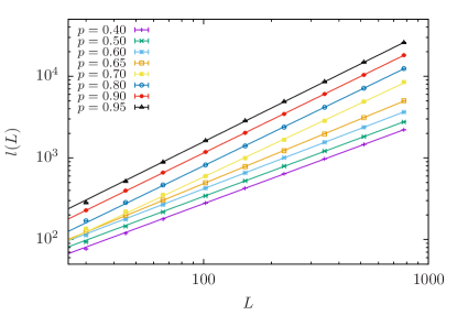
Figure 7: (Color online) Domain wall length $l$ at different system sizes $L$. The straight lines are power-law fits to the data sets.

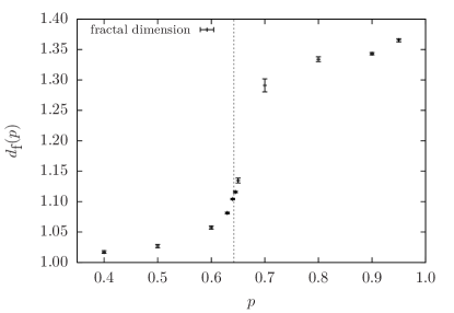
Figure 8: (Color online) Fractal dimension $d_{\text{f}}$ of the domain wall length at different occupancy $p$. The vertical dashed line marks the critical point $p_{\text{c}}=0.6423(3)$.

The property which is discussed last is the DW energy. The same $10,000$ samples used for the domain wall length are analyzed here. This results in the data shown in Fig. 9.

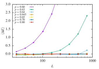
Figure 9: (Color online) Average domain wall energy at different system sizes. Data points are connected using straight lines for better visibility.

The data was plotted on a semi-log scale, since some average values are negative. For occupancy $p<0.645$ the average DW energy increases linearly. This includes values of $p<0.6$ which were omitted from the plot for a clearer image. This indicates a sub lattice ferromagnetic, i.e., globally antiferromagnetic, phase, where introduction of a DW breaks the long range order and costs energy. This behavior is expected for occupancy smaller than the critical point $p_{\text{c}}$, since the system is antiferromagnetic at $p=0$. For $p\geq 0.645$ the DW energy is roughly zero, which is typical for both possibilities of a paramagnetic and a spin-glass phase. Note that fairly large system sizes are required, as the $p=0.63$ curve is also approximately zero at first, but then increases around $L=100$. Similarly, the $p=0.64$ curve only deviates from zero around $L=600$. This means that systems around these occupancy values may appear not sub lattice ferromagnetically ordered at small system sizes. Further transitions at greater values of $p$ and much larger systems sizes cannot be fully excluded from this plot, but are unlikely, as we found the critical point to be $p_{\text{c}}=0.6423(3)$.

To determine whether there exists a spin-glass phase, we look at the standard deviation of the DW energy in Fig. 10.

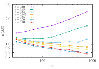
Figure 10: (Color online) Standard deviation of domain wall energy at different system sizes. Data points are connected using straight lines for better visibility.

Again, the curves split into two categories: Increasing standard deviation with the system size at $p<0.645$ and decreasing values at $p\geq 0.645$. This suggests that the ferromagnetic phase is stable at finite temperatures, but the claimed spin-glass phase only exists at $T=0$. For a stable spin-glass phase the standard deviation would have to increase in some region of the $p\geq 0.645$ range, which is clearly not observed. With these results it can be concluded that previous reports of a stable $T_{\text{c}}>0$ spin-glass phase are not supported by our results.

V Conclusions

We have numerically studied the Kaya-Berker model, with a site occupancy $p$ of one sublattice, by using an exact ground state algorithm. Thus, we were able to obtain $T=0$ results in exact equilibrium. Since the ground-state calculation is equivalent to obtain a minimum-weight perfect matching, it is possible to obtain ground states with a running time growing only polynomially in system size. Therefore, we were able to study very large system sizes of up to $\sim 10^{5}$ lattice sites.

From the obtained GSs, we calculated the magnetization and the corresponding Binder parameter as a function of the occupancy $p$. Here we used a slight randomization of the bonds to obtain a almost unbiased sampling of the degenerate ground states. From the Binder parameter, we obtained a critical value $p_{c}=0.6423(3)$ where the sublattice magnetization vanishes. This value is considerably smaller than previous results. Nevertheless, the previous results were obtained by using methods which involve approximations, non-equilibrium sampling often without a guarantee of convergence and they were restricted to small system sizes. Therefore, our results are much more reliable than those obtained from the previous studies. Although there might be a slight bias from the sampling of the ground states, from the comparison of the results for the pure samples and the randomized samples, as well as from the previous results for the random bond (spin-glass) model, we know that his influence is very small, much smaller than the discrepancy to the previous results.

We also studied domain walls which are obtained by comparing the GS of the original realizations with periodic boundary conditions in $x$-direction and the GS of the realization with antiperiodic boundary conditions. By analyzing the length of the domain-walls and its dependence on the system size, we obtained the fractal dimension. The result for the fractal dimension as a function of the occupancy shows a fractal dimension of basically one in the phase where the sublattice magnetization is non-zero. Close to the point a strong increase of the fractal dimension can be observed, supporting the results for the phase transition obtained from the magnetization.

The results for scaling of the average DW energy are also compatible with a transition at the location $p_{c}$ where the magnetization vanishes. The variance of the DW energy distribution changes from growing to shrinking with the system size $L$ at (or close to) the same point $p_{c}$. Thus, it is rather likely, that the Kaya-Berker model does not exhibit a spin-glass phase at a low but finite temperature, because this would have to go together with a decrease of the mean value and an increase of the variance with the system size at the same time at some values of $p$.

To conclude, so far for no two-dimensional (random) frustrated Ising systems with short-range nearest neighbor interactions a low-temperature spin-glass phase with a finite critical temperature has been found (although for some it had been claimed before). To conclude, it still remains an open question whether such a system exists, but is appears to be unlikely to the authors.