Gravitational Waves, $\mu$ Term & Leptogenesis from $B-L$ Higgs Inflation in Supergravity

Abstract

We consider a renormalizable extension of the minimal supersymmetric standard model endowed by an $R$ and a gauged $B-L$ symmetry. The model incorporates chaotic inflation driven by a quartic potential, associated with the Higgs field which leads to a spontaneous breaking of $U(1)_{B-L}$, and yields possibly detectable gravitational waves. We employ quadratic Kähler potentials with a prominent shift-symmetric part proportional to $c_{-}$ and a tiny violation, proportional to $c_{+}$, included in a logarithm with prefactor $-N<0$. An explanation of the $\mu$ term of the MSSM is also provided, consistently with the low energy phenomenology, under the condition that one related parameter in the superpotential is somewhat small. Baryogenesis occurs via non-thermal leptogenesis which is realized by the inflaton’s decay to the lightest or next-to-lightest right-handed neutrino with masses lower than $1.8\cdot 10^{13}~{}{\mbox{\rm GeV}}$. Our scenario can be confronted with the current data on the inflationary observables, the baryon asymmetry of the universe, the gravitino limit on the reheating temperature and the data on the neutrino oscillation parameters, for $0.012\lesssim c_{+}/c_{-}\lesssim 1/N$ and gravitino as light as $1~{}{\mbox{\rm TeV}}$.

Keywords: Cosmology, Inflation, Supersymmetric Models
PACS codes: 98.80.Cq, 12.60.Jv, 95.30.Cq, 95.30.Sf

Published in Universe 4, no. 1, 13 (2018)

1 Introduction

One of the primary ideas, followed the introduction of inflation [3] as a solution to longstanding cosmological problems – such as the horizon, flatness and magnetic monopoles problems –, was its connection with a phase transition related to the breakdown of a Grand Unified Theory (GUT). According to this economical and highly appealing scenario – called henceforth Higgs inflation (HI) – the inflaton may be identified with one particle involved in the Higgs sector [4, 7, 6, 5, 8, 9] of a GUT model. In a series of recent papers [10, 11] we established a novel type of GUT-scale, mainly, HI called kinetically modified non-Minimal HI. This term is coined in Ref. [12] due to the fact that, in the non-Supersymmetric (SUSY) set-up, this inflationary model, based on the $\phi^{4}$ power-law potential, employs not only a suitably selected non-minimal coupling to gravity $f_{\cal R}=1+c_{+}\phi^{2}$ but also a kinetic mixing of the form $f_{\rm K}=c_{-}f_{\cal R}^{m}$ – cf. Ref. [13]. The merits of this construction compared to the original (and certainly more predictive) model [4, 14, 15] of non-minimal inflation (nMI) defined for $f_{\rm K}=1$ are basically two:

• For $m\geq 0$, the observables depend on the ratio $r_{\pm}=c_{+}/c_{-}$ and can be done excellently consistent with the the recent data [16, 17] as regards the tensor-to-scalar ratio, $r$. More specifically, all data taken by the Bicep2/Keck Array CMB polarization experiments up to and including the 2014 observing season (BK14) [17] seem to favor $r$’s of order $0.01$, since the analysis yields

  $$r=0.028^{+0.026}_{-0.025}~{}~{}\Rightarrow~{}~{}0.003\lesssim r\lesssim 0.054\hskip 5.69046pt\mbox{at 68\%c.l.}$$ (1)

• The resulting theory respects the perturbative unitarity [18, 19] up to the Planck scale for $r_{\pm}\leq 1$ and $m$ of order unity.

In the SUSY – which means Supergravity (SUGRA) – framework the two ingredients necessary to achieve this kind of nMI, i.e., the non-minimal kinetic mixing and coupling to gravity, originate from the same function, the Kähler potential, and the set-up becomes much more attractive. Actually, the non-minimal kinetic mixing and gravitational coupling of the inflaton can be elegantly realized introducing an approximate shift symmetry [20, 21, 13, 22, 10]. Namely, the constants $c_{-}$ and $c_{+}$ introduced above can be interpreted as the coefficients of the principal shift-symmetric term ($c_{-}$) and its violation ($c_{+}$) in the Kähler potentials $K$. Allowing also for a variation of the coefficients of the logarithms appearing in the $K$’s we end up with the most general form of these models analyzed in Ref. [11].

Here, we firstly single out the most promising models from those investigated in Ref. [11], employing as a guiding principle the consistency of the expansion of the $K$’s in powers of the various fields. Namely, as we mention in Ref. [11], $m=0$ and $m=1$ are the two most natural choices since they require just quadratic terms in some of the $K$’s considered. From these two choices the one with $m=1$ is privileged since it ensures $r$ within Eq. (1) with central value for the spectral index $n_{\rm s}$. Armed with the novel stabilization mechanisms for the non-inflaton accompanied field – recently proposed in the context of the Starobinsky-type inflation [23] too –, we concentrate here on $K$’s including exclusively quadratic terms with $m=1$. The embedding of the selected models in a complete framework is the second aim of this paper. Indeed, a complete inflationary model should specify the transition to the radiation domination, explain the origin of the observed baryon asymmetry of the universe (BAU) [24] and also, yield the minimal supersymmetric standard model (MSSM) as low energy theory. Although this task was carried out for similar models – see, e.g., Refs. [6, 25, 26] – it would be certainly interesting to try to adapt it to the present set-up. Further restrictions are induced from this procedure.

A GUT based on $G_{B-L}=G_{\rm SM}\times U(1)_{B-L}$, where ${G_{\rm SM}}=SU(3)_{\rm C}\times SU(2)_{\rm L}\times U(1)_{Y}$ is the gauge group of the standard model and $B$ and $L$ denote the baryon and lepton number respectively, consists [22, 10, 11] a conveniently simple framework which allows us to exemplify our proposal. Actually, this is a minimal extension of the MSSM which is obtained by promoting the already existing $U(1)_{B-L}$ global symmetry to a local one. The Higgs fields which cause the spontaneous breaking of the $G_{B-L}$ symmetry to ${G_{\rm SM}}$ can naturally play the role of inflaton. This breaking provides large Majorana masses to the right-handed neutrinos, $N^{c}_{i}$, whose the presence is imperative in order to cancel the gauge anomalies and generate the tiny neutrino masses via the seesaw mechanism. Furthermore, the out-of-equilibrium decay of the $N^{c}_{i}$’s provides us with an explanation of the observed BAU [27] via non-thermal leptogenesis (nTL) [28] consistently with the gravitino ($\widetilde{G}$) constraint [29, 30, 31, 32] and the data [33, 34] on the neutrino oscillation parameters. As a consequence, finally, of an adopted global $R$ symmetry, the parameter $\mu$ appearing in the mixing term between the two electroweak Higgs fields in the superpotential of MSSM is explained as in Refs. [35, 25] via the vacuum expectation value (v.e.v) of the non-inflaton accompanying field, provided that the relevant coupling constant is rather suppressed.

Below, we present the particle content, the superpotential and the possible Kähler potentials which define our model in Sec. 2. In Sec. 3 we describe the inflationary potential, derive the inflationary observables and confront them with observations. Sec. 4 is devoted to the resolution of the $\mu$ problem of MSSM. In Sec. 5 we analyze the scenario of nTL exhibiting the relevant constraints and restricting further the parameters. Our conclusions are summarized in Sec. 6. Throughout the text, the subscript of type $,z$ denotes derivation with respect to (w.r.t) the field $z$ and charge conjugation is denoted by a star. Unless otherwise stated, we use units where $m_{\rm P}=2.433\cdot 10^{18}~{}{\mbox{\rm GeV}}$ is taken unity.

2 Model Description

We focus on an extension of MSSM invariant under the gauge group $G_{B-L}$. Besides the MSSM particle content, the model is augmented by six superfields: a gauge singlet $S$, three $N^{c}_{i}$’s, and a pair of Higgs fields $\Phi$ and $\bar{\Phi}$ which break $U(1)_{B-L}$. In addition to the local symmetry, the model possesses also the baryon and lepton number symmetries and a nonanomalous $R$ symmetry $U(1)_{R}$. The charge assignments under these symmetries of the various matter and Higgs superfields are listed in Table 1. We below present the superpotential (Sec. 2.1) and (some of) the Kähler potentials (Sec. 2.2) which give rise to our inflationary scenario.

2.1 Superpotential

The superpotential of our model naturally splits into two parts:

$$W=W_{\rm MSSM}+W_{\rm HI},\>\>\>\mbox{where}$$ (2)

(a)

$W_{\rm MSSM}$ is the part of $W$ which contains the usual terms – except for the $\mu$ term – of MSSM, supplemented by Yukawa interactions among the left-handed leptons ($L_{i}$) and $N^{c}_{i}$:

$$W_{\rm MSSM}=h_{ijD}{d}^{c}_{i}{Q}_{j}{H_{d}}+h_{ijU}{u}^{c}_{i}{Q}_{j}{H_{u}}+h_{ijE}{e}^{c}_{i}{L}_{j}{H_{d}}+h_{ijN}N^{c}_{i}L_{j}{H_{u}}.$$ (3a)

Here the $$i SU(2)_{\rm L} Q_{i} L_{i} SU(2)_{\rm L} u^{c}_{i} {d_{i}}^{c} e^{c}_{i} N^{c}_{i} {H_{u}} {H_{d}}$$th generation doublet left-handed quark and lepton superfields are denoted by and respectively, whereas the singlet antiquark [antilepton] superfields by and [ and ] respectively. The electroweak Higgs superfields which couple to the up [down] quark superfields are denoted by [].

(b)

$W_{\rm HI}$ is the part of $W$ which is relevant for HI, the generation of the $\mu$ term of MSSM and the Majorana masses for $N^{c}_{i}$’s. It takes the form

$$W_{\rm HI}=\lambda S\left(\bar{\Phi}\Phi-M^{2}/4\right)+\lambda_{\mu}S{H_{u}}{H_{d}}+\lambda_{[N^{c}}i]\bar{\Phi}N^{c2}_{i}\,.$$ (3b)

The imposed $U(1)_{R}$ symmetry ensures the linearity of $W_{\rm HI}$ w.r.t $S$. This fact allows us to isolate easily via its derivative the contribution of the inflaton into the F-term SUGRA potential, placing $S$ at the origin – see Sec. 3.1. It plays also a key role in the resolution of the $\mu$ problem of MSSM via the second term in the right-hand side (r.h.s) of Eq. (3b) – see Sec. 4.2. The inflaton is contained in the system $\bar{\Phi}-\Phi$. We are obliged to restrict ourselves to subplanckian values of $\bar{\Phi}\Phi$ since the imposed symmetries do not forbid non-renormalizable terms of the form $(\bar{\Phi}\Phi)^{p}$ with $p>1$ – see Sec. 3.3. The third term in the r.h.s of Eq. (3b) provides the Majorana masses for the $N^{c}_{i}$’s – cf. Refs. [6, 25, 26] – and assures the decay [36] of the inflaton to $\widetilde{N}_{i}^{c}$, whose subsequent decay can activate nTL. Here, we work in the so-called $N^{c}_{i}$-basis, where $M_{[N^{c}}i]$ is diagonal, real and positive. These masses, together with the Dirac neutrino masses in Eq. (3a), lead to the light neutrino masses via the seesaw mechanism.

Superfields	Representations	Global Symmetries
	under $G_{B-L}$	$R$	$B$	$L$
Matter Fields
$e^{c}_{i}$	$({\bf 1,1},1,1)$	$1$	$0$	$-1$
$N^{c}_{i}$	$({\bf 1,1},0,1)$	$1$	$0$	$-1$
$L_{i}$	$({\bf 1,2},-1/2,-1)$	$1$	$0$	$1$
$u^{c}_{i}$	$({\bf 3,1},-2/3,-1/3)$	$1$	$-1/3$	$0$
$d^{c}_{i}$	$({\bf 3,1},1/3,-1/3)$	$1$	$-1/3$	$0$
$Q_{i}$	$({\bf\bar{3},2},1/6,1/3)$	$1$	$1/3$	$0$
Higgs Fields
${H_{d}}$	$({\bf 1,2},-1/2,0)$	$0$	$0$	$0$
${H_{u}}$	$({\bf 1,2},1/2,0)$	$0$	$0$	$0$
$S$	$({\bf 1,1},0,0)$	$2$	$0$	$0$
$\Phi$	$({\bf 1,1},0,2)$	$0$	$0$	$-2$
$\bar{\Phi}$	$({\bf 1,1},0,-2)$	$0$	$0$	$2$

Table 1: The representations under $G_{B-L}$ and the extra global charges of the superfields of our model.

2.2 Kähler Potentials

HI is feasible if $W_{\rm HI}$ cooperates with one of the following Kähler potentials – cf. Ref. [11]:

$$K_{1} = -N\ln\left(1+c_{+}F_{+}+F_{1X}(|X|^{2})\right)+c_{-}F_{-},$$ (4a)

$$K_{2} = -N\ln\left(1+c_{+}F_{+}\right)+c_{-}F_{-}+F_{2X}(|X|^{2}),$$ (4b)

$$K_{3} = -N\ln\left(1+c_{+}F_{+}\right)+F_{3X}(F_{-},|X|^{2}),$$ (4c)

where $N>0$, $X^{\gamma}=S,{H_{u}},{H_{d}},\widetilde{N}_{i}^{c}$ and the complex scalar components of the superfields $\Phi,\bar{\Phi},S,{H_{u}}$ and ${H_{d}}$ are denoted by the same symbol whereas this of $N^{c}_{i}$ by $\widetilde{N}_{i}^{c}$. The functions $F_{\pm}=\left|\Phi\pm\bar{\Phi}^{*}\right|^{2}$ assist us in the introduction of shift symmetry for the Higgs fields – cf. Ref. [21, 22]. In all $K$’s, $F_{+}$ is included in the argument of a logarithm with coefficient $-N$ whereas $F_{-}$ is outside it. As regards the non-inflaton fields $X^{\gamma}$, we assume that they have identical kinetic terms expressed by the functions $F_{lX}$ with $l=1,2,3$. In Table 2 we expose two possible forms for each $F_{lX}$ following Ref. [23]. These are selected so as to successfully stabilize the scalars $X^{\gamma}$ at the origin employing only quadratic terms. Recall [37, 23] that the simplest term $|X|^{2}$ leads to instabilities for $K=K_{1}$ and light excitations of $X^{\gamma}$ for $K=K_{2}$ and $K_{3}$. The heaviness of these modes is required so that the observed curvature perturbation is generated wholly by our inflaton in accordance with the lack of any observational hint [27] for large non-Gaussianity in the cosmic microwave background.

As we show in Sec. 3.1, the positivity of the kinetic energy of the inflaton sector requires $c_{+}<c_{-}$ and $N>0$. For $r_{\pm}=c_{+}/c_{-}\ll 1$, our models are completely natural in the ’t Hooft sense because, in the limits $c_{+}\rightarrow 0$ and $\lambda\rightarrow 0$, they enjoy the following enhanced symmetries

$$\Phi\rightarrow\ \Phi+c,\>\>\>\bar{\Phi}\rightarrow\ \bar{\Phi}+c^{*}\>\>\>\mbox{and}\>\>\>X^{\gamma}\rightarrow\ e^{i\varphi_{\gamma}}X^{\gamma},$$ (5)

where $c$ and $\varphi_{\gamma}$ are complex and real numbers respectively and no summation is applied over $\gamma$. This enhanced symmetry has a string theoretical origin as shown in Ref. [38]. In this framework, mainly integer $N$’s are considered which can be reconciled with the observational data. Namely, acceptable inflationary solutions are attained for $N=3$ [$N=2$] if $K=K_{1}$ [$K=K_{2}$ or $K_{3}$] – see Sec. 3.4. However, deviation of the $N$’s from these integer values is perfectly acceptable [22, 11, 40, 39] and can have a pronounced impact on the inflationary predictions allowing for a covering of the whole $n_{\rm s}-r$ plane with quite natural values of the relevant parameters.

3 Inflationary Scenario

The salient features of our inflationary scenario are studied at tree level in Sec. 3.1 and at one-loop level in Sec. 3.2. We then present its predictions in Sec. 3.4, calculating a number of observable quantities introduced in Sec. 3.3.

$F_{lX}$	Exponential Form	Logarithmic Form
$F_{1X}$	$\exp\left(-|X|^{2}/N\right)-1$	$-\ln(1+|X|^{2}/N)$
$F_{2X}$	$-N_{X}\left(\exp\left(-|X|^{2}/N_{X}\right)-1\right)$	$N_{X}\ln(1+|X|^{2}/N_{X})$
$F_{3X}$	$-N_{X}\left(\exp\left(-c_{-}F_{-}/N_{X}-|X|^{2}/N_{X}\right)-1\right)$	$N_{X}\ln(1+c_{-}F_{-}/N_{X}+|X|^{2}/N_{X})$

Table 2: Functional forms of $F_{lX}$ with $l=1,2,3$ shown in the definition of $K_{1},K_{2}$ and $K_{3}$ in Eqs. (4a), (4b) and (4c) respectively.

3.1 Inflationary Potential

Within SUGRA the Einstein frame (EF) action for the scalar fields $z^{\alpha}=S,\Phi,\bar{\Phi},{H_{u}},{H_{d}}$ and $\widetilde{N}_{i}^{c}$ can be written as

$${\sf S}=\int d^{4}x\sqrt{-\widehat{\mathfrak{g}}}\left(-\frac{1}{2}\widehat{\mathcal{R}}+K_{{\alpha}{\bar{\beta}}}\widehat{g}^{\mu\nu}D_{\mu}z^{\alpha}D_{\nu}z^{*{\bar{\beta}}}-\widehat{V}\right),$$ (6a)

where $$\widehat{\mathcal{R}} \mathfrak{g} g^{\mu\nu} (+,-,-,-)$$ is the Ricci scalar and is the determinant of the background Friedmann-Robertson-Walker metric, with signature . We adopt also the following notation

$$K_{{\alpha}{\bar{\beta}}}={K_{,z^{\alpha}z^{*{\bar{\beta}}}}}>0\>\>\>\mbox{and}\>\>\>D_{\mu}z^{\alpha}=\partial_{\mu}z^{\alpha}+igA^{\rm a}_{\mu}T^{\rm a}_{{\alpha}{\beta}}z^{\beta}$$ (6b)

are the covariant derivatives for the scalar fields $$z^{\alpha} g A^{\rm a}_{\mu} T^{\rm a} z^{\alpha} \widehat{V}$$. Also, is the unified gauge coupling constant, are the vector gauge fields and are the generators of the gauge transformations of . Also is the EF SUGRA scalar potential which can be found via the formula

$$\widehat{V}=\widehat{V}_{\rm F}+\widehat{V}_{\rm D}\>\>\>\mbox{with}\>\>\>\widehat{V}_{\rm F}=e^{K}\left(K^{{\alpha}{\bar{\beta}}}D_{\alpha}W_{\rm HI}D^{*}_{\bar{\beta}}W_{\rm HI}^{*}-3{|W_{\rm HI}|^{2}}\right)\>\>\>\mbox{and}\>\>\>\widehat{V}_{\rm D}={1\over 2}g^{2}\sum_{\rm a}{\rm D}_{\rm a}{\rm D}_{\rm a},$$ (6c)

where we use the notation

$$K^{{\alpha}{\bar{\beta}}}K_{{\alpha}\bar{\gamma}}=\delta^{\bar{\beta}}_{\bar{\gamma}},\>\>D_{\alpha}W_{\rm HI}=W_{{\rm HI},z^{\alpha}}+K_{{\alpha}}W_{\rm HI}~{}~{}\mbox{and}~{}~{}{\rm D}_{\rm a}=z^{\alpha}\left(T_{\rm a}\right)_{\alpha}^{\beta}K_{\beta}~{}~{}\mbox{with}~{}~{}K_{{\alpha}}={K_{,z^{\alpha}}}.$$ (6d)

If we express $\Phi,\bar{\Phi}$ and $X^{\gamma}=S,{H_{u}},{H_{d}},\widetilde{N}_{i}^{c}$ according to the parametrization

$$\Phi=\frac{\phi e^{i{\theta}}}{\sqrt{2}}\cos{\theta_{\Phi}},~{}~{}\bar{\Phi}=\frac{\phi e^{i{\bar{\theta}}}}{\sqrt{2}}\sin{\theta_{\Phi}}~{}~{}\mbox{and}~{}~{}X^{\gamma}=\frac{x^{\gamma}+i\bar{x}^{\gamma}}{\sqrt{2}}\,,$$ (7)

where $0\leq{\theta_{\Phi}}\leq\pi/2$, we can easily deduce from Eq. (6c) that a D-flat direction occurs at

$$x^{\gamma}=\bar{x}^{\gamma}={\theta}={\bar{\theta}}=0\>\>\>\mbox{and}\>\>\>{\theta_{\Phi}}={\pi/4}$$ (8)

along which the only surviving term in Eq. (6c) can be written universally as

$$\widehat{V}_{\rm HI}=e^{K}K^{SS^{*}}\,|W_{{\rm HI},S}|^{2}=\frac{\lambda^{2}(\phi^{2}-M^{2})^{2}}{16f_{\cal R}^{2(1+n)}}\>\>\>\mbox{where}\>\>\>f_{\cal R}=1+c_{+}\phi^{2}$$ (9)

plays the role of a non-minimal coupling to Ricci scalar in the Jordan frame (JF) – see Refs. [37, 22]. Also, we set

$$n=\left\{\begin{matrix}(N-3)/2\hfill\cr N/2-1\hfill\cr\end{matrix}\right.\>\>\>\mbox{and}\>\>\>K^{SS^{*}}=\left\{\begin{matrix}f_{\cal R}\hfill\cr 1\hfill\cr\end{matrix}\right.\>\>\>\mbox{for}\>\>\>\left\{\begin{matrix}K=K_{1}\,,\hfill\cr K=K_{2}~{}~{}\mbox{and}~{}~{}K_{3}\,.\hfill\cr\end{matrix}\right.$$ (10)

The introduction of $n$ allows us to obtain a unique inflationary potential for all the $K$’s in Eqs. (4a) – (4c). For $K=K_{1}$ and $N=3$ or $K=K_{2}$ or $K_{3}$ and $N=2$ we get $n=0$ and $\widehat{V}_{\rm HI}$ develops an inflationary plateau as in the original case of non-minimal inflation [4]. Contrary to that case, though, here we have also $c_{-}$ which dominates the canonical normalization of $\phi$ – see Sec. 3.2 – and allows for distinctively different inflationary outputs as shown in Refs. [12, 10]. Finally, the variation of $n$ above and below zero allows for more drastic deviations [22, 11] from the predictions of the original model [4]. In particular, for $n<0$, $\widehat{V}_{\rm HI}$ remains increasing function of $\phi$, whereas for $n>0$, $\widehat{V}_{\rm HI}$ develops a local maximum

$$\widehat{V}_{\rm HI}(\phi_{\rm max})=\frac{\lambda^{2}n^{2n}}{16c_{+}^{2}(1+n)^{2(1+n)}}~{}~{}\mbox{at}~{}~{}\phi_{\rm max}=\frac{1}{\sqrt{c_{+}n}}\,.$$ (11)

In a such case we are forced to assume that hilltop [41] HI occurs with $\phi$ rolling from the region of the maximum down to smaller values. Therefore, a mild tuning of the initial conditions is required which can be quantified somehow defining [42] the quantity

$$\Delta_{\rm max\star}=\left(\phi_{\rm max}-\phi_{\star}\right)/\phi_{\rm max}\,,$$ (12)

$\phi_{\star}$ is the value of $\phi$ when the pivot scale $k_{\star}=0.05/{\rm Mpc}$ crosses outside the inflationary horizon. The naturalness of the attainment of HI increases with $\Delta_{\rm max\star}$ and it is maximized when $\phi_{\rm max}\gg\phi_{\star}$ which result to $\Delta_{\rm max\star}\simeq 1$.

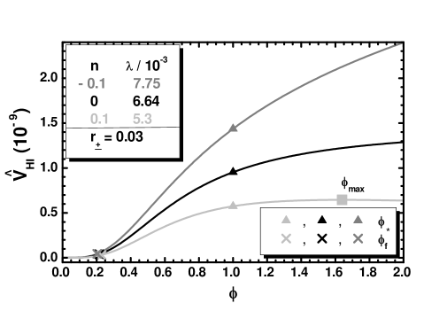
Figure 1: The inflationary potential $\widehat{V}_{\rm HI}$ as a function of $\phi$ for $\phi>0$, and $r_{\pm}\simeq 0.03$, and $n=-0.1$, $\lambda=7.75\cdot 10^{-3}$ (gray line), $n=0$, $\lambda=6.64\cdot 10^{-3}$ (black line), or $n=+0.1$, $\lambda=5.3\cdot 10^{-3}$ (light gray line). The values of $\phi_{\star}$, $\phi_{\rm f}$ and $\phi_{\rm max}$ (for $n=1/10$) are also indicated.

The structure of $\widehat{V}_{\rm HI}$ as a function of $\phi$ is displayed in Fig. 1. We take $\phi_{\star}=1$, $r_{\pm}=0.03$ and $n=-0.1$ (light gray line), $n=0$ (black line) and $n=0.1$ (gray line). Imposing the inflationary requirements mentioned in Sec. 3.4 we find the corresponding values of $\lambda$ and $c_{-}$ which are $(7.75,6.64~{}{\rm or}~{}5.3)\cdot 10^{-3}$ and $(1.7,1.46,{\rm or}~{}1.24)\cdot 10^{2}$ respectively. The corresponding observable quantities are found numerically to be $n_{\rm s}=0.971,0.969$ or $0.966$ and $r=0.045,0.03$ or $0.018$ with $a_{\rm s}\simeq-5\cdot 10^{-4}$ in all cases. We see that $\widehat{V}_{\rm HI}$ is a monotonically increasing function of $\phi$ for $n\leq 0$ whereas it develops a maximum at $\phi_{\rm max}=1.64$, for $n=0.1$, which leads to a mild tuning of the initial conditions of HI since $\Delta_{\rm max\star}=39\%$, according to the criterion introduced above. It is also remarkable that $r$ increases with the inflationary scale, $\widehat{V}_{\rm HI}^{1/4}$, which, in all cases, approaches the SUSY GUT scale $M_{\rm GUT}\simeq 8.2\cdot 10^{-3}$ facilitating the interpretation of the inflaton as a GUT-scale Higgs field.

3.2 Stability and one-Loop Radiative Corrections

As deduced from Eq. (9) $\widehat{V}_{\rm HI}$ is independent from $c_{-}$ which dominates, though, the canonical normalization of the inflaton. To specify it together with the normalization of the other fields, we note that, for all $K$’s in Eqs. (4a) – (4c), $K_{{\alpha}{\bar{\beta}}}$ along the configuration in Eq. (8) takes the form

$$\left(K_{{\alpha}{\bar{\beta}}}\right)={\sf diag}\left(M_{\pm},\underbrace{K_{\gamma\bar{\gamma}},...,K_{\gamma\bar{\gamma}}}_{8~{}\mbox{\footnotesize elements}}\right)$$ (13a)

with

$$M_{\pm}=\frac{1}{f_{\cal R}^{2}}\mbox{ $\left\lgroup\begin{matrix}\kappa&\bar{\kappa}\cr\bar{\kappa}&\kappa\end{matrix}\right\rgroup$}~{}~{}\mbox{and}~{}~{}K_{\gamma\bar{\gamma}}=\left\{\begin{matrix}1/f_{\cal R}\hfill\cr 1\hfill\cr\end{matrix}\right.\>\>\>\mbox{for}\>\>\>\left\{\begin{matrix}K=K_{1}\,,\hfill\cr K=K_{2}~{}~{}\mbox{and}~{}~{}K_{3}\,.\hfill\cr\end{matrix}\right.$$ (13b)

Here $\kappa=c_{-}f_{\cal R}^{2}-Nc_{+}$ and $\bar{}\kappa={Nc_{+}^{2}\phi^{2}}$. Upon diagonalization of $M_{\pm}$ we find its eigenvalues which are

$$\kappa_{+}=c_{-}\left(1+Nr_{\pm}(c_{+}\phi^{2}-1)/{f_{\cal R}^{2}}\right)\simeq c_{-}\>\>\>\mbox{and}\>\>\>\kappa_{-}=c_{-}\left(1-{Nr_{\pm}}/{f_{\cal R}}\right),$$ (14)

where the positivity of $\kappa_{-}$ is assured during and after HI for

$$r_{\pm}<f_{\cal R}/N~{}~{}\mbox{with}~{}~{}r_{\pm}=c_{+}/c_{-}\,.$$ (15)

Given that $f_{\cal R}>1$ and $\langle{f_{\cal R}}\rangle\simeq 1$, Eq. (15) implies that the maximal possible $r_{\pm}$ is $r_{\pm}^{\rm max}\simeq 1/N$. Given that $N$ tends to $3$ [$2$] for $K=K_{1}$ [$K=K_{2}$ or $K_{3}$], the inequality above discriminates somehow the allowed parameter space for the various choices of $K$’s in Eqs. (4a) – (4b).

Inserting Eqs. (7) and (13b) in the second term of the r.h.s of Eq. (6a) we can, then, specify the EF canonically normalized fields, which are denoted by hat, as follows

$$K_{{\alpha}{\bar{\beta}}}\dot{z}^{\alpha}\dot{z}^{*{\bar{\beta}}} = {\kappa_{+}\over 2}\left(\dot{}\phi^{2}+{1\over 2}\phi^{2}\dot{\theta}^{2}_{+}\right)+{\kappa_{-}\over 2}\phi^{2}\left({1\over 2}\dot{\theta}^{2}_{-}+\dot{\theta}^{2}_{\Phi}\right)+\frac{1}{2}K_{\gamma\bar{\gamma}}\left(\dot{x}^{\gamma 2}+\dot{\bar{x}}^{\gamma 2}\right)$$ (16a)

$$\simeq \frac{1}{2}\left(\dot{\widehat{}\phi}^{~{}2}+\dot{\widehat{\theta}}_{+}^{~{}2}+\dot{\widehat{{\theta}}}_{-}^{~{}2}+\dot{\widehat{\theta}}_{\Phi}^{~{}2}+\dot{\widehat{x}}^{\gamma 2}+\dot{\widehat{\bar{x}}}^{~{}~{}\gamma 2}\right),$$

where $${\theta}_{\pm}=\left(\bar{\theta}\pm{\theta}\right)/\sqrt{2} t \Phi-\bar{\Phi}$$ and the dot denotes derivation w.r.t the cosmic time . The hatted fields of the system can be expressed in terms of the initial (unhatted) ones via the relations

$$\frac{d\widehat{\phi}}{d\phi}=J=\sqrt{\kappa_{+}},\>\>\widehat{\theta}_{+}={J\over\sqrt{2}}\phi\theta_{+},\>\>\widehat{\theta}_{-}=\sqrt{\frac{\kappa_{-}}{2}}\phi\theta_{-},\>\>\mbox{and}\>\>\widehat{\theta}_{\Phi}=\sqrt{\kappa_{-}}\phi\left(\theta_{\Phi}-\frac{\pi}{4}\right)\,\cdot$$ (16b)

As regards the non-inflaton fields, the (approximate) normalization is implemented as follows

$$(\widehat{x}^{\gamma},\widehat{\bar{x}}^{\gamma})=\sqrt{K_{\gamma\bar{\gamma}}}(x^{\gamma},\bar{x}^{\gamma}).$$ (16c)

As we show below, the masses of the scalars besides $\widehat{\phi}$ during HI are heavy enough such that the dependence of the hatted fields on $\phi$ does not influence their dynamics – see also Ref. [6].

We can verify that the inflationary direction in Eq. (8) is stable w.r.t the fluctuations of the non-inflaton fields. To this end, we construct the mass-squared spectrum of the scalars taking into account the canonical normalization of the various fields in Eq. (16a) – for details see Ref. [22]. In the limit $c_{-}\gg c_{+}$, we find the expressions of the masses squared $\widehat{m}^{2}_{z^{\alpha}}$ (with $z^{\alpha}=\theta_{+},\theta_{\Phi},x^{\gamma}$ and $\bar{x}^{\gamma}$) arranged in Table 3. These results approach rather well the quite lengthy, exact expressions taken into account in our numerical computation. The various unspecified there eigenvalues are defined as follows

$$h_{\pm}=(h_{u}\pm{h_{d}})/\sqrt{2},\>\>\>{\bar{h}}_{\pm}=({\bar{h}}_{u}\pm{\bar{h}}_{d})/\sqrt{2}\>\>\>\mbox{and}\>\>\>\widehat{\psi}_{\pm}=(\widehat{\psi}_{\Phi+}\pm\widehat{\psi}_{S})/\sqrt{2},$$ (17a)

where the (unhatted) spinors $$\psi_{\Phi} \psi_{\bar{\Phi}} \Phi \bar{\Phi}$$ and associated with the superfields and are related to the normalized (hatted) ones in Table 3 as follows

$$\widehat{\psi}_{\Phi\pm}=\sqrt{\kappa_{\pm}}\psi_{\Phi\pm}\>\>\>\mbox{with}\>\>\>\psi_{\Phi\pm}=(\psi_{\Phi}\pm\psi_{\bar{\Phi}})/\sqrt{2}\,.$$ (17b)

From Table 3 it is evident that $0<{N_{X}}\leq 6$ assists us to achieve $m^{2}_{{s}}>\widehat{H}_{\rm HI}^{2}=\widehat{V}_{\rm HI}/3$ – in accordance with the results of Ref. [23] – and also enhances the ratios $m^{2}_{X^{\tilde{\gamma}}}/\widehat{H}_{\rm HI}^{2}$ for $X^{\tilde{\gamma}}={H_{u}},{H_{d}},\widetilde{N}_{i}^{c}$ w.r.t the values that we would have obtained, if we had used just canonical terms in the $K$’s. On the other hand, $\widehat{m}^{2}_{h-}>0$ requires

$$\lambda_{\mu}<\lambda(1+c_{+}\phi^{2}/N)/4\left(1/\phi^{2}+c_{+}\right) ~{}~{}\mbox{for}~{}~{}K=K_{1};$$ (18a)

$$\lambda_{\mu}<\lambda\phi^{2}(1+1/{N_{X}})/4 ~{}~{}\mbox{for}~{}~{}K=K_{2}~{}~{}\mbox{and}~{}~{}K_{3}\,.$$ (18b)

In both cases, the quantity in the r.h.s of the inequality takes its minimal value at $\phi=\phi_{\rm f}$ and numerically equals to $2\cdot 10^{-5}-10^{-6}$. Similar numbers are obtained in Ref. [25] although that higher order terms in the Kähler potential are invoked there. We do not consider such a condition on $\lambda_{\mu}$ as unnatural, given that $h_{1U}$ in Eq. (3a) is of the same order of magnitude too – cf. Ref. [43]. Note that the due hierarchy in Eqs. (18a) and (18b) between $\lambda_{\mu}$ and $\lambda$ differs from that imposed in the models [35] of F-term hybrid inflation, where $S$ plays the role of inflaton and $\Phi,\bar{\Phi},~{}{H_{u}}$ and ${H_{d}}$ are confined at zero. Indeed, in that case we demand [35] $\lambda_{\mu}>\lambda$ so that the tachyonic instability in the $\Phi-\bar{\Phi}$ direction occurs first, and the $\Phi-\bar{\Phi}$ system start evolving towards its v.e.v, whereas ${H_{u}}$ and ${H_{d}}$ continue to be confined to zero. In our case, though, the inflaton is included in the $\bar{\Phi}-\Phi$ system while $S$ and the ${H_{u}}-{H_{d}}$ system are safely stabilized at the origin both during and after HI. Therefore, $\phi$ is led at its vacuum whereas $S$, ${H_{u}}$ and ${H_{d}}$ take their non-vanishing electroweak scale v.e.vs afterwards.

Fields	Eigen-	Masses Squared
	states		$K=K_{1}$	$K=K_{2}$	$K=K_{3}$
14 Real	$\widehat{\theta}_{+}$	$\widehat{m}_{\theta+}^{2}$	$6\widehat{H}_{\rm HI}^{2}$		$6(1+1/{N_{X}})\widehat{H}_{\rm HI}^{2}$
Scalars	$\widehat{\theta}_{\Phi}$	$\widehat{m}_{\theta_{\Phi}}^{2}$	$M^{2}_{BL}+6\widehat{H}_{\rm HI}^{2}$		$M^{2}_{BL}+6(1+1/{N_{X}})\widehat{H}_{\rm HI}^{2}$
	$\widehat{s},\widehat{\bar{s}}$	$\widehat{m}_{s}^{2}$	$6c_{+}\phi^{2}\widehat{H}_{\rm HI}^{2}/N$	$6\widehat{H}_{\rm HI}^{2}/{N_{X}}$
	$\widehat{h}_{\pm},\widehat{\bar{h}}_{\pm}$	$\widehat{m}_{h\pm}^{2}$	$3\widehat{H}_{\rm HI}^{2}\left(1+{c_{+}\phi^{2}}/{N}\pm{4\lambda_{\mu}}(1/{\phi^{2}}+c_{+})/{\lambda}\right)$	$3\widehat{H}_{\rm HI}^{2}\left(1+1/{N_{X}}\pm{4\lambda_{\mu}}/{\lambda\phi^{2}}\right)$
	$\widehat{\tilde{\nu}}^{c}_{i},\widehat{\bar{\tilde{\nu}}}^{c}_{i}$	$\widehat{m}_{i\tilde{\nu}^{c}}^{2}$	$3\widehat{H}_{\rm HI}^{2}\left(1+{c_{+}\phi^{2}}/{N}+{16\lambda^{2}_{iN^{c}}}(1/{\phi^{2}}+c_{+})/{\lambda^{2}}\right)$	$3\widehat{H}_{\rm HI}^{2}\left(1+1/{N_{X}}+16\lambda^{2}_{iN^{c}}/\lambda^{2}\phi^{2}\right)$
1 Gauge Boson	$A_{BL}$	$M_{BL}^{2}$	$g^{2}c_{-}\left(1-Nr_{\pm}/f_{\cal R}\right)\phi^{2}$
$7$ Weyl	$\widehat{\psi}_{\pm}$	$\widehat{m}^{2}_{\psi\pm}$	$6\left((N-3)c_{+}\phi^{2}-2\right)^{2}\widehat{H}_{\rm HI}^{2}/c_{-}\phi^{2}f_{\cal R}^{2}$	$6\left((N-2)c_{+}\phi^{2}-2\right)^{2}\widehat{H}_{\rm HI}^{2}/c_{-}\phi^{2}f_{\cal R}^{2}$
Spinors	${N_{i}^{c}}$	$\widehat{m}_{{iN^{c}}}^{2}$	$48\lambda^{2}_{iN^{c}}\widehat{H}_{\rm HI}^{2}/\lambda^{2}\phi^{2}$
	$\uplambda_{BL},\widehat{\psi}_{\Phi-}$	$M_{BL}^{2}$	$g^{2}c_{-}\left(1-Nr_{\pm}/f_{\cal R}\right)\phi^{2}$

Table 3: The mass squared spectrum of our models along the inflationary trajectory in Eq. (8) for $K=K_{1},K_{2},K_{3}$ and $\phi\ll 1$. To avoid very lengthy formulas, we neglect terms proportional to $M\ll\phi$.

In Table 3 we display also the mass $M_{BL}$ of the gauge boson which becomes massive having ‘eaten’ the Goldstone boson ${\theta}_{-}$. This signals the fact that $G_{B-L}$ is broken during HI. Shown are also the masses of the corresponding fermions – note that the fermions $\tilde{h}_{\pm}$ and $\tilde{\bar{h}}_{\pm}$, associated with $h_{\pm}$ and $\bar{h}_{\pm}$ remain massless. The derived mass spectrum can be employed in order to find the one-loop radiative corrections, $\Delta\widehat{V}_{\rm HI}$ to $\widehat{V}_{\rm HI}$. Considering SUGRA as an effective theory with cutoff scale equal to $m_{\rm P}$, the well-known Coleman-Weinberg formula [44] can be employed self-consistently taking into account the masses which lie well below $m_{\rm P}$, i.e., all the masses arranged in Table 3 besides $M_{BL}$ and $\widehat{m}_{{\theta}_{\Phi}}$. Therefore, the one-loop correction to $\widehat{V}_{\rm HI}$ reads

$$\Delta\widehat{V}_{\rm HI} = {1\over 64\pi^{2}}\left(\widehat{m}_{{\theta}+}^{4}\ln{\widehat{m}_{{\theta}+}^{2}\over\Lambda^{2}}+2\widehat{m}_{s}^{4}\ln{\widehat{m}_{s}^{2}\over\Lambda^{2}}+4\widehat{m}_{h+}^{4}\ln{\widehat{m}_{h+}^{2}\over\Lambda^{2}}+4\widehat{m}_{h-}^{4}\ln{\widehat{m}_{h-}^{2}\over\Lambda^{2}}\right.$$ (19)

$$+ \left.2\sum_{i=1}^{3}\left(\widehat{m}_{i\tilde{\nu}^{c}}^{4}\ln{\widehat{m}_{i\tilde{\nu}^{c}}^{2}\over\Lambda^{2}}-\widehat{m}_{iN^{c}}^{4}\ln{\widehat{m}_{iN^{c}}^{2}\over\Lambda^{2}}\right)-4\widehat{m}_{\psi_{\pm}}^{4}\ln{\widehat{m}_{\psi_{\pm}}^{2}\over\Lambda^{2}}\right),$$

where $\Lambda$ is a renormalization group (RG) mass scale. The resulting $\Delta\widehat{V}_{\rm HI}$ lets intact our inflationary outputs, provided that $\Lambda$ is determined by requiring $\Delta\widehat{V}_{\rm HI}(\phi_{\star})=0$ or $\Delta\widehat{V}_{\rm HI}(\phi_{\rm f})=0$. These conditions yield $\Lambda\simeq 3.2\cdot 10^{-5}-1.4\cdot 10^{-4}$ and render our results practically independent of $\Lambda$ since these can be derived exclusively by using $\widehat{V}_{\rm HI}$ in Eq. (9) with the various quantities evaluated at $\Lambda$ – cf. Ref. [22]. Note that their renormalization-group running is expected to be negligible because $\Lambda$ is close to the inflationary scale $\widehat{V}_{\rm HI}^{1/4}\simeq(3-7)\cdot 10^{-3}$ – see Fig. 1.

3.3 Inflationary Observables

A period of slow-roll HI is determined by the condition – see e.g. Ref. [45]

$${\footnotesize\sf max}\{\widehat{\epsilon}(\phi),|\widehat{\eta}(\phi)|\}\leq 1,$$ (20)

where

$$\widehat{\epsilon}={1\over 2}\left(\frac{\widehat{V}_{{\rm HI},\widehat{\phi}}}{\widehat{V}_{\rm HI}}\right)^{2}={1\over 2J^{2}}\left(\frac{\widehat{V}_{{\rm HI},\phi}}{\widehat{V}_{\rm HI}}\right)^{2}\simeq\frac{8(1-nc_{+}\phi^{2})^{2}}{c_{-}\phi^{2}f_{\cal R}^{2}}$$ (21a)

and

$$\widehat{\eta}=\frac{\widehat{V}_{{\rm HI},\widehat{\phi}\widehat{\phi}}}{\widehat{V}_{\rm HI}}={1\over J^{2}}\left(\frac{\widehat{V}_{{\rm HI},\phi\phi}}{\widehat{V}_{\rm HI}}-\frac{\widehat{V}_{{\rm HI},\phi}}{\widehat{V}_{\rm HI}}{J_{,\phi}\over J}\right)=4\>\frac{3-3(1+3n)c_{+}\phi^{2}+n(1+4n)c_{+}^{2}\phi^{4}}{c_{-}\phi^{2}f_{\cal R}^{2}}\,\cdot$$ (21b)

Expanding $\widehat{\epsilon}$ and $\widehat{\eta}$ for $\phi\ll 1$ we can find from Eq. (20) that HI terminates for $\phi=\phi_{\rm f}$ such that

$$\phi_{\rm f}\simeq\mbox{\footnotesize\sf max}\left\{\frac{2\sqrt{2/c_{-}}}{\sqrt{1+16(1+n)r_{\pm}}},\frac{2\sqrt{3/c_{-}}}{\sqrt{1+36(1+n)r_{\pm}}}\right\}.$$ (22)

The number of e-foldings, ${\widehat{N}_{\star}}$, that the pivot scale $k_{\star}=0.05/{\rm Mpc}$ suffers during HI can be calculated through the relation

$${\widehat{N}_{\star}}=\>\int_{\widehat{\phi}_{\rm f}}^{\widehat{\phi}_{\star}}\,d\widehat{\phi}\>\frac{\widehat{V}_{\rm HI}}{\widehat{V}_{\rm HI,\widehat{\phi}}}\simeq\begin{cases}({(1+c_{+}\phi_{\star}^{2})^{2}-1})/{16r_{\pm}}~{}~{}&\mbox{for}~{}~{}n=0\,,\\ -\left({nc_{+}\phi_{\star}^{2}+(1+n)\ln(1-nc_{+}\phi_{\star}^{2})}\right)/{8n^{2}r_{\pm}}~{}~{}&\mbox{for}~{}~{}n\neq 0\,,\end{cases}$$ (23)

where $\widehat{\phi}_{\star}$ is the value of $\widehat{\phi}$ when $k_{\star}$ crosses the inflationary horizon. As regards the consistency of the relation above for $n>0$, we note that we get $nc_{+}\phi_{\star}^{2}<1$ in all relevant cases and so, $\ln(1-nc_{+}\phi_{\star}^{2})<0$ assures the positivity of ${\widehat{N}_{\star}}$. Given that $\phi_{\rm f}\ll\phi_{\star}$, we can write $\phi_{\star}$ as a function of ${\widehat{N}_{\star}}$ as follows

$$\phi_{\star}\simeq{\sqrt{f_{n\star}-1\over c_{+}}}~{}~{}\mbox{with}~{}~{}f_{n\star}=\begin{cases}\left(1+16r_{\pm}{\widehat{N}_{\star}}\right)^{1/2}~{}~{}&\mbox{for}~{}~{}n=0\,,\\ \left((1+n)/n\right)\left(1+W_{k}\left({y/(1+n)}\right)\right)~{}~{}&\mbox{for}~{}~{}n\neq 0\,.\end{cases}$$ (24)

Here $W_{k}$ is the Lambert $W$ or product logarithmic function [46] and the parameter $y$ is defined as $y=-\exp\left(-(1+8n^{2}{\widehat{N}_{\star}}r_{\pm})/(1+n)\right)$. We take $k=0$ for $n\geq 0$ and $k=-1$ for $n<0$. We can impose a lower bound on $c_{-}$ above which $\phi_{\star}\leq 1$ for every $r_{\pm}$. Indeed, from Eq. (24) we have

$$\phi_{\star}\leq 1~{}~{}\Rightarrow~{}~{}c_{-}\geq{\left(f_{n\star}-1\right)}/{r_{\pm}}$$ (25)

and so, our proposal can be stabilized against corrections from higher order terms of the form $(\Phi\bar{\Phi})^{p}$ with $p>1$ in $W_{\rm HI}$ – see Eq. (3b). Despite the fact that $c_{-}$ may take relatively large values, the corresponding effective theory is valid up to $m_{\rm P}=1$ – contrary to the pure quartic nMI [18, 19]. To clarify further this point we have to identify the ultraviolet cut-off scale $\Lambda_{\rm UV}$ of theory analyzing the small-field behavior of our models. More specifically, we expand about $\langle{\phi}\rangle=M\ll 1$ the second term in the r.h.s of Eq. (6a) for $\mu=\nu=0$ and $\widehat{V}_{\rm HI}$ in Eq. (9). Our results can be written in terms of $\widehat{\phi}$ as

$$J^{2}\dot{\phi}^{2} \simeq \left(1+3Nr_{\pm}^{2}\widehat{\phi}^{2}-5Nr_{\pm}^{3}\widehat{\phi}^{4}+\cdots\right)\dot{}\widehat{\phi}^{2};$$ (26a)

$$\widehat{V}_{\rm HI} \simeq \frac{\lambda^{2}\widehat{\phi}^{4}}{16c_{-}^{2}}\left(1-2(1+n)r_{\pm}\widehat{\phi}^{2}+(3+5n)r_{\pm}^{2}\widehat{\phi}^{4}-\cdots\right)\,.$$ (26b)

From the expressions above we conclude that $\Lambda_{\rm UV}=m_{\rm P}$ since $r_{\pm}\leq 1$ due to Eq. (15). Although the expansions presented above, are valid only during reheating we consider the extracted $\Lambda_{\rm UV}$ as the overall cut-off scale of the theory since the reheating is regarded [19] as an unavoidable stage of HI.

The power spectrum $A_{\rm s}$ of the curvature perturbations generated by $\phi$ at the pivot scale $k_{\star}$ is estimated as follows

$$\sqrt{A_{\rm s}}=\>\frac{1}{2\sqrt{3}\,\pi}\;\frac{\widehat{V}_{\rm HI}(\widehat{\phi}_{\star})^{3/2}}{|\widehat{V}_{\rm HI,\widehat{\phi}}(\widehat{\phi}_{\star})|}\simeq\frac{\lambda\sqrt{c_{-}}}{32\sqrt{3}\pi}\frac{\phi_{\star}^{3}f_{\cal R}(\phi_{\star})^{-n}}{1-nc_{+}\phi_{\star}^{2}}\,\cdot$$ (27)

The resulting relation reveals that $\lambda$ is proportional to $c_{-}$ for fixed $n$ and $r_{\pm}$. Indeed, plugging Eq. (24) into the expression above, we find

$$\lambda=32\sqrt{3A_{\rm s}}\pi c_{-}r_{\pm}^{3/2}f_{n\star}^{n}\frac{n(1-f_{n\star})+1}{(f_{n\star}-1)^{3/2}}\,\cdot$$ (28)

At the same pivot scale, we can also calculate $n_{\rm s}$, its running, $a_{\rm s}$, and $r$ via the relations

$$n_{\rm s}=\>1-6\widehat{\epsilon}_{\star}\ +\ 2\widehat{\eta}_{\star}\simeq 1-4n^{2}r_{\pm}-2n\frac{r_{\pm}^{1/2}}{{\widehat{N}_{\star}}^{1/2}}-\frac{3-2n}{2{\widehat{N}_{\star}}}-\frac{3-n}{8({\widehat{N}_{\star}}^{3}r_{\pm})^{1/2}}\,,\>\>\>$$ (29a)

$$a_{\rm s}=\>{2\over 3}\left(4\widehat{\eta}_{\star}^{2}-(n_{\rm s}-1)^{2}\right)-2\widehat{\xi}_{\star}\simeq-\frac{nr_{\pm}^{1/2}}{{\widehat{N}_{\star}}^{3/2}}-\frac{3-2n}{2{\widehat{N}_{\star}}^{2}},$$ (29b)

$$r=16\widehat{\epsilon}_{\star}\simeq-\frac{8n}{{\widehat{N}_{\star}}}+\frac{3+2n}{6{\widehat{N}_{\star}}^{2}r_{\pm}}+\frac{6-n}{3({\widehat{N}_{\star}}^{3}r_{\pm})^{1/2}}+\frac{8n^{2}r_{\pm}^{1/2}}{{\widehat{N}_{\star}}^{1/2}}\,,$$ (29c)

where $\widehat{\xi}={\widehat{V}_{\rm HI,\widehat{}\phi}\widehat{V}_{\rm HI,\widehat{}\phi\widehat{}\phi\widehat{}\phi}/\widehat{V}_{\rm HI}^{2}}$ and the variables with subscript $\star$ are evaluated at $\phi=\phi_{\star}$.

3.4 Comparison with Observations

The approximate analytic expressions above can be verified by the numerical analysis of our model. Namely, we apply the accurate expressions in Eqs. (23) and (27) and confront the corresponding observables with the requirements [27]

$$\mbox{\footnotesize\sf(a)}\>\>{\widehat{N}_{\star}}\simeq 61.5+\ln{\widehat{V}_{\rm HI}(\phi_{\star})^{1/2}\over\widehat{V}_{\rm HI}(\phi_{\rm f})^{1/4}}+\frac{1}{2}f_{\cal R}(\phi_{\star})~{}~{}~{}\mbox{and}~{}~{}~{}\mbox{\footnotesize\sf(b)}\>\>A_{\rm s}^{1/2}\simeq 4.627\cdot 10^{-5}\,.$$ (30)

We, thus, restrict $\lambda$ and $\phi_{\star}$ and compute the model predictions via Eqs. (29a), (29b) and (29c) for any selected $n$ and $r_{\pm}$. In Eq. (30a) we consider an equation-of-state parameter $w_{\rm int}=1/3$ correspoding to quartic potential which is expected to approximate rather well $\widehat{V}_{\rm HI}$ for $\phi\ll 1$. For rigorous comparison with observations we compute $r_{0.002}=16\widehat{\epsilon}(\widehat{\phi}_{0.002})$ where $\widehat{\phi}_{0.002}$ is the value of $\widehat{\phi}$ when the scale $k=0.002/{\rm Mpc}$, which undergoes $\widehat{N}_{0.002}={\widehat{N}_{\star}}+3.22$ e-foldings during HI, crosses the horizon of HI. These must be in agreement with the fitting of the Planck, Baryon Acoustic Oscillations (BAO) and Bicep2/Keck Array data [16, 17] with $\Lambda$CDM$+r$ model, i.e.,

$$\mbox{\footnotesize\sf(a)}\>\>n_{\rm s}=0.968\pm 0.009\>\>\>~{}\mbox{and}\>\>\>~{}\mbox{\footnotesize\sf(b)}\>\>r\leq 0.07,$$ (31)

at 95$\%$ confidence level (c.l.) with $|a_{\rm s}|\ll 0.01$.

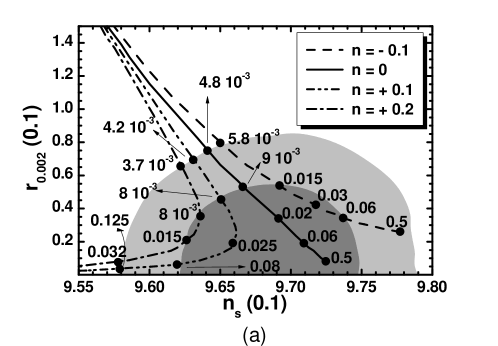
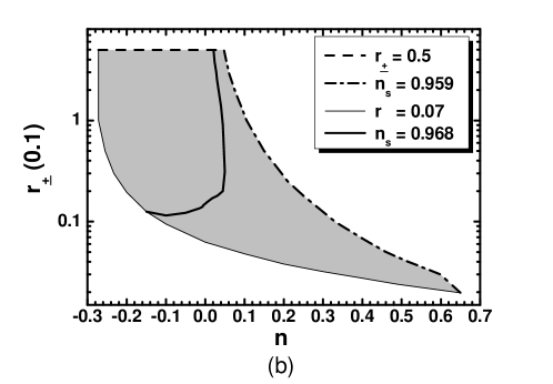
Figure 2: (a) Allowed curves in the $n_{\rm s}-r_{0.002}$ plane for $K=K_{2}$ and $K_{3}$, $n=-0.1,0,0.1,0.2$ with the $r_{\pm}$ values indicated on the curves – the marginalized joint $68\%$ [$95\%$] regions from Planck, BAO and BK14 data are depicted by the dark [light] shaded contours. (b) Allowed (shaded) regions in the $n-r_{\pm}$ plane for $K=K_{2}$ and $K_{3}$. The conventions adopted for the various lines are shown.

Let us clarify here that the free parameters of our models are $n$, $r_{\pm}$ and $\lambda/c_{-}$ and not $n$, $c_{-}$, $c_{+}$ and $\lambda$ as naively expected. Indeed, if we perform the rescalings

$$\Phi\rightarrow\Phi/\sqrt{c_{-}},~{}~{}\bar{\Phi}\rightarrow\bar{\Phi}/\sqrt{c_{-}}~{}~{}~{}\mbox{and}~{}~{}~{}S\rightarrow S,$$ (32)

$W$ in Eq. (3b) depends on $\lambda/c_{-}$ and the $K$’s in Eq. (4a) – (4c) depend on $n$ and $r_{\pm}$. As a consequence, $\widehat{V}_{\rm HI}$ depends exclusively on $\lambda/c_{-}$, $n$ and $r_{\pm}$. Since the $\lambda/c_{-}$ variation is rather trivial – see Ref. [10] – we focus on the variation of the other parameters.

Our results are displayed in Fig. 2. Namely, in Fig. 2-(a) we show a comparison of the models’ predictions against the observational data [16, 17] in the $n_{\rm s}-r_{0.002}$ plane. We depict the theoretically allowed values with dot-dashed, double dot-dashed, solid and dashed lines for $n=0.2,0.1,0$ and $-0.1$ respectively. The variation of $r_{\pm}$ is shown along each line. For low enough $r_{\pm}$’s – i.e. $r_{\pm}\leq 0.0005$ – the various lines converge to $(n_{\rm s},r_{0.002})\simeq(0.947,0.28)$ obtained within minimal quartic inflation defined for $c_{+}=0$. Increasing $r_{\pm}$ the various lines enter the observationally allowed regions, for $r_{\pm}$ equal to a minimal value $r_{\pm}^{\rm min}$, and cover them. The lines corresponding to $n=0,-0.1$ terminate for $r_{\pm}=r_{\pm}^{\rm max}\simeq 0.5$, beyond which Eq. (15) is violated. Finally, the lines drawn with $n=0.2$ or $n=0.1$ cross outside the allowed corridors and so the $r_{\pm}^{\rm max}$’s, are found at the intersection points. From Fig. 2-(a) we infer that the lines with $n>0$ [$n<0$] cover the left lower [right upper] corner of the allowed range. As we anticipated in Sec. 3.1, for $n>0$ HI is of hilltop type. The relevant parameter $\Delta_{\rm max\star}$ ranges from $0.07$ to $0.66$ for $n=0.1$ and from $0.19$ to $0.54$ for $n=0.2$ where $\Delta_{\rm max\star}$ increases as $r_{\pm}$ drops. That is, the required tuning is not severe mainly for $r_{\pm}<0.1$.

As deduced from Fig. 2-(a), the observationally favored region can be wholly filled varying conveniently $n$ and $r_{\pm}$. It would, therefore, interesting to delineate the allowed region of our models in the $n-r_{\pm}$ plane, as shown in Fig. 2-(b). The conventions adopted for the various lines are also shown in the legend of the plot. In particular, the allowed (shaded) region is bounded by the dashed line, which originates from Eq. (15), and the dot-dashed and thin lines along which the lower and upper bounds on $n_{\rm s}$ and $r$ in Eq. (31) are saturated respectively. We remark that increasing $r_{\pm}$ with $n=0$, $r$ decreases, in accordance with our findings in Fig. 2-(a). On the other hand, $r_{\pm}$ takes more natural – in the sense of the discussion at the end of Sec. 2.2 – values (lower than unity) for larger values of $|n|$ where hilltop HI is activated. Fixing $n_{\rm s}$ to its central value in Eq. (31a) we obtain the thick solid line along which we get clear predictions for $(n,r_{\pm})$ and so, the remaining inflationary observables. Namely, we find

$$-1.21\lesssim{n\over 0.1}\lesssim 0.215,\>\>\>0.12\lesssim{r_{\pm}\over 0.1}\lesssim 5,\>\>\>0.4\lesssim{r\over 0.01}\lesssim 7\>\>\>\mbox{and}\>\>\>0.25\lesssim 10^{5}{\lambda\over c_{-}}\lesssim 2.6\,.$$ (33)

Hilltop HI is attained for $0<n\leq 0.0215$ and there, we get $\Delta_{\rm max\star}\gtrsim 0.4$. The parameter $a_{\rm s}$ is confined in the range $-(5-6)\cdot 10^{-4}$ and so, our models are consistent with the fitting of data with the $\Lambda$CDM+$r$ model [16]. Moreover, our models are testable by the forthcoming experiments like Bicep3 [47], PRISM [48] and LiteBIRD [49] searching for primordial gravity waves since $r\gtrsim 0.0019$.

Had we employed $K=K_{1}$, the various lines ended at $r_{\pm}\simeq 0.5$ in Fig. 2-(a) and the allowed region in Fig. 2-(b) would have been shortened until $r_{\pm}\simeq 0.33$. This bound would have yielded slightly larger $r_{0.002}^{\rm min}$’s. Namely, $r_{0.002}^{\rm min}\simeq 0.0084$ or $0.026$ for $n=0$ or $-0.1$ respectively – the $r_{0.002}^{\rm min}$’s for $n>0$ are let unaffected. The lower bound of $r/0.01$ and the upper ones on $r_{\pm}/0.1$ and $10^{5}\lambda/c_{-}$ in Eq. (33) become $0.64$, $3.3$ and $2.1$ whereas the bounds on $a_{\rm s}$ remain unaltered.

4 Higgs Inflation and $\mu$ Term of MSSM

A byproduct of the $R$ symmetry associated with our model is that it assists us to understand the origin of $\mu$ term of MSSM. To see how this works, we first – in Sec. 4.1 – derive the SUSY potential of our models, and then – in Sec. 4.2 – we study the generation of the $\mu$ parameter and investigate the possible consequences for the phenomenology of MSSM – see Sec. 4.3. Here and henceforth we restore units, i.e., we take $m_{\rm P}=2.433\cdot 10^{18}~{}{\mbox{\rm GeV}}$.

4.1 SUSY Potential

Since $\widehat{V}_{\rm HI}$ in Eq. (9) is non-renormalizable, its SUSY limit $V_{\rm SUSY}$ depends not only on $W_{\rm HI}$ in Eq. (3b), but also on the $K$’s in Eqs. (4a) – (4c). In particular, $V_{\rm SUSY}$ turns out to be [50]

$$V_{\rm SUSY}=\widetilde{K}^{{\alpha}{\bar{\beta}}}W_{\rm HI{\alpha}}W^{*}_{\rm HI{\bar{\beta}}}+\frac{g^{2}}{2}\mbox{$\sum_{\rm a}$}{\rm D}_{\rm a}{\rm D}_{\rm a}\,,$$ (34a)

where $$\widetilde{K} K m_{\rm P}\rightarrow\infty$$ is the limit of the aforementioned ’s for which is

$$\widetilde{K}=c_{-}F_{-}-Nc_{+}F_{+}+|S|^{2}+|{H_{u}}|^{2}+|{H_{d}}|^{2}+|\widetilde{N}_{i}^{c}|^{2}\,.$$ (34b)

Upon substitution of $$\widetilde{K}$$ into Eq. (34a) we obtain

$$V_{\rm SUSY}=\lambda^{2}\left|\bar{\Phi}\Phi-\frac{1}{4}{M^{2}}+\frac{\lambda_{\mu}}{\lambda}{H_{u}}{H_{d}}\right|^{2}+\frac{1}{c_{-}(1-Nr_{\pm})}\left(\left|\lambda S\Phi+\lambda_{iN^{c}}\widetilde{N}^{c2}\right|^{2}+\lambda^{2}|S\bar{\Phi}|^{2}\right)+$$

$$\lambda_{\mu}^{2}|S|^{2}\left(|{H_{u}}|^{2}+|{H_{d}}|^{2}\right)+4\lambda_{iN^{c}}^{2}|\bar{\Phi}\widetilde{N}_{i}^{c}|^{2}+\frac{g^{2}}{2}\left(c_{-}(1-Nr_{\pm})\left(|\Phi|^{2}-|\bar{\Phi}|^{2}\right)+|\widetilde{N}_{i}^{c}|^{2}\right)^{2}\,.$$ (34c)

From the last equation, we find that the SUSY vacuum lies along the D-flat direction $|\bar{\Phi}|=|\Phi|$ with

$$\langle{S}\rangle=\langle{{H_{u}}}\rangle=\langle{{H_{d}}}\rangle=\langle{\widetilde{N}_{i}^{c}}\rangle=0\>\>\>\mbox{and}\>\>\>|\langle{\Phi}\rangle|=|\langle{\bar{\Phi}}\rangle|=M/2\,.$$ (35)

As a consequence, $\langle{\Phi}\rangle$ and $\langle{\bar{\Phi}}\rangle$ break spontaneously $U(1)_{B-L}$ down to $\mathbb{Z}^{B-L}_{2}$. Since $U(1)_{B-L}$ is already broken during HI, no cosmic string are formed – contrary to what happens in the models of the standard F-term hybrid inflation [5, 35, 42], which employ $W_{\rm HI}$ in Eq. (3b) too.

4.2 Generation of the $\mu$ Term of MSSM

The contributions from the soft SUSY breaking terms, although negligible during HI, since these are much smaller than $\phi$, may shift [35, 25] slightly $\langle{S}\rangle$ from zero in Eq. (35). Indeed, the relevant potential terms are

$$V_{\rm soft}=\left(\lambda A_{\lambda}S\bar{\Phi}\Phi+\lambda_{\mu}A_{\mu}S{H_{u}}{H_{d}}+\lambda_{iN^{c}}A_{iN^{c}}\Phi\widetilde{N}^{c2}_{i}-{\rm a}_{S}S\lambda M^{2}/4+{\rm h.c.}\right)+m_{\gamma}^{2}\left|X^{\gamma}\right|^{2},$$ (36)

where $m_{\gamma},A_{\lambda},A_{\mu},A_{iN^{c}}$ and ${\rm a}_{S}$ are soft SUSY breaking mass parameters. Rotating $S$ in the real axis by an appropriate $R$-transformation, choosing conveniently the phases of $A_{\lambda}$ and ${\rm a}_{S}$ so as the total low energy potential $V_{\rm tot}=V_{\rm SUSY}+V_{\rm soft}$ to be minimized – see Eq. (34c) – and substituting in $V_{\rm soft}$ the SUSY v.e.vs of $\Phi,\bar{\Phi},{H_{u}},{H_{d}}$ and $N^{c}_{i}$ from Eq. (35) we get

$$\langle{V_{\rm tot}(S)}\rangle=\lambda^{2}\,M^{2}S^{2}/2c_{-}(1-Nr_{\pm})-\lambda{\rm a}_{3/2}m_{3/2}M^{2}S,$$ (37a)

where we take into account that $$m_{S}\ll M |A_{\lambda}|+|{\rm a}_{S}|=2{\rm a}_{3/2}m_{3/2} m_{3/2} \widetilde{G} {\rm a}_{3/2}>0 |A_{\lambda}| |{\rm a}_{S}| m_{3/2} S \langle{S}\rangle$$ and we set with being the mass and a parameter of order unity which parameterizes our ignorance for the dependence of and on . The minimization condition for the total potential in Eq. (37a) w.r.t leads to a non vanishing as follows

$$\frac{d}{dS}\langle{V_{\rm tot}(S)}\rangle=0~{}~{}\Rightarrow~{}~{}\langle{S}\rangle\simeq{\rm a}_{3/2}m_{3/2}c_{-}(1-Nr_{\pm})/\lambda.$$ (37b)

At this $$S \langle{V_{\rm tot}(S)}\rangle$$ value, develops a minimum since

$$\frac{d^{2}}{dS^{2}}\langle{V_{\rm tot}(S)}\rangle=\lambda^{2}\,M^{2}/c_{-}(1-Nr_{\pm})$$ (37c)

becomes positive for $r_{\pm}<1/N$, as dictated by Eq. (15). Let us emphasize here that SUSY breaking effects explicitly break $U(1)_{R}$ to the $\mathbb{Z}_{2}^{R}$ matter parity, under which all the matter (quark and lepton) superfields change sign. Combining $\mathbb{Z}_{2}^{R}$ with the $\mathbb{Z}_{2}^{\rm f}$ fermion parity, under which all fermions change sign, yields the well-known $R$-parity. Recall that this residual symmetry prevents the rapid proton decay, guarantees the stability of the lightest SUSY particle (LSP) and therefore, it provides a well-motivated cold dark matter (CDM) candidate. Since $S$ has the $R$ symmetry of $W$, $\langle{S}\rangle$ in Eq. (37b) breaks also spontaneously $U(1)_{R}$ to $\mathbb{Z}_{2}^{R}$. Thanks to this fact, $\mathbb{Z}_{2}^{R}$ remains unbroken and so, no disastrous domain walls are formed.

The generated $\mu$ term from the second term in the r.h.s of Eq. (3b) is

$$\mu=\lambda_{\mu}\langle{S}\rangle\simeq\lambda_{\mu}{\rm a}_{3/2}m_{3/2}c_{-}(1-Nr_{\pm})/\lambda$$ (38a)

which, taking into account Eq. (28), is written as

$$\mu\simeq 1.2\cdot 10^{2}\lambda_{\mu}{\rm a}_{3/2}m_{3/2}(1-Nr_{\pm})r_{\pm}^{-3/2}f_{n\star}^{-n}\frac{(f_{n\star}-1)^{3/2}}{n(1-f_{n\star})+1}\,,$$ (38b)

where $c_{-}$ and $\lambda$ are eliminated. As a consequence, the resulting $\mu$ in Eq. (38a) depends on $r_{\pm}$ and $n$ but does not depend on $\lambda$ and $c_{-}$ – in contrast to the originally proposed scheme in Ref. [35] where a $\lambda$ dependence remains. Note, also, that $\lambda_{\mu}$ (and so $\mu$) may have either sign without any essential alteration in the stability analysis of the inflationary system – see Table 3. Thanks to the magnitude of the proportionality constant and given that $r_{\pm}^{-3/2}$ turns out to be about $10^{3}$ for $r_{\pm}$ of order $0.01$, as indicated by Fig. 2, we conclude that any $|\mu|$ value is accessible for the $\lambda_{\mu}$ values allowed by Eqs. (18a) and (18b) without any ugly hierarchy between $m_{3/2}$ and $\mu$.

To highlight further the statement above, we can employ Eq. (38a) to derive the $m_{3/2}$ values required so as to obtain a specific $\mu$ value. E.g., we fix $\mu=1~{}{\mbox{\rm TeV}}$ as suggested by many MSSM versions for acceptable low energy phenomenology – see Ref. [51]. Given that Eq. (38a) dependents on $r_{\pm}$ and $n$, which crucially influences $n$ and $r$, we expect that the required $m_{3/2}$ is a function of $n$ and $r$ as depicted in Fig. 3-(a) and Fig. 3-(b) respectively. We take $\lambda_{\mu}=10^{-6}$, in accordance with Eqs. (18a) and (18b), ${\rm a}_{3/2}=1$, $K=K_{2}$ or $K_{3}$ with ${N_{X}}=2$ and $n=-0.1$ (dot-dashed line), $n=0$ (solid line), or $n=+0.1$ (dashed line). Varying $r_{\pm}$ in the allowed ranges indicated in Fig. 2-(a) for any of the $n$’s above we obtain the variation of $m_{3/2}$ solving Eq. (38a) w.r.t $m_{3/2}$. We see that $m_{3/2}\geq 1.6~{}{\mbox{\rm TeV}}$ with the lowest value obtained for $n=0.1$. Also, $m_{3/2}$ corresponding to $n=0$ and $-0.1$ increases sharply as $r_{\pm}$ approaches $0.49$ due to the denominator $1-Nr_{\pm}$ which approaches zero. Had we used $K=K_{1}$ this enhancement would have been occurred as $r_{\pm}$ tends to $0.33$.

Obviously the proposed resolution of the $\mu$ problem of MSSM relies on the existence of non-zero $A_{\lambda}$ and/or ${\rm a}_{S}$. These issues depend on the adopted model of SUSY breaking. Here we have in mind mainly the gravity mediated SUSY breaking without, though, to specify the extra terms in the superpotential and the Kähler potentials which ensure the appropriate soft SUSY breaking parameters and the successful stabilization of the sgolstino – cf. Ref. [52]. Since this aim goes beyond the framework of this work, we restrict ourselves to assume that these terms can be added without disturbing the inflationary dynamics.

4.3 Connection with the MSSM Phenomenology

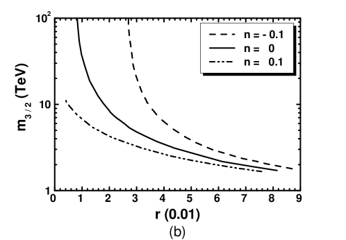
Figure 3: The gravitino mass $m_{3/2}$ versus $n_{\rm s}$ (a) or $r$ (b) for $\mu=1~{}{\mbox{\rm TeV}},\lambda_{\mu}=10^{-6}$, ${\rm a}_{3/2}=1$, $K=K_{2}$ or $K_{3}$ with ${N_{X}}=2$ and $n=-0.1$ (dot-dashed line), $n=0$ (solid line), or $n=+0.1$ (dashed line).

Taking advantage from the updated investigation of the parameter space of Constrained MSSM (CMSSM) in Ref. [51] we can easily verify that the $\mu$ and $m_{3/2}$ values satisfying Eq. (38a) are consistent with the values required by the analyses of the low energy observables of MSSM. We concentrate on CMSSM which is the most predictive, restrictive and well-motivated version of MSSM, employing the free parameters

$${\rm sign}\mu,~{}~{}\tan\beta=\langle{{H_{u}}}\rangle/\langle{{H_{d}}}\rangle,~{}~{}{M_{1/2}},~{}~{}m_{0}~{}~{}\mbox{and}~{}~{}A_{0},$$

where ${\rm sign}\mu$ is the sign of $\mu$, and the three last mass parameters denote the common gaugino mass, scalar mass, and trilinear coupling constant, respectively, defined at a high scale which is determined by the unification of the gauge coupling constants. The parameter $|\mu|$ is not free, since it is computed at low scale enforcing the conditions for the electroweak symmetry breaking. The values of these parameters can be tightly restricted imposing a number of cosmo-phenomenological constraints. Namely, these constraints originate from the cold dark matter abundance in the universe and its direct detection experiments, the $B$-physics, as well as the masses of the sparticles and the lightest neutral CP-even Higgs boson. Some updated results are recently presented in Ref. [51], where we can also find the best-fit values of $|A_{0}|$, $m_{0}$ and $|\mu|$ listed in Table 4. We see that there are four allowed regions characterized by the specific mechanism for suppressing the relic density of the lightest sparticle which can act as dark matter. If we identify $m_{0}$ with $m_{3/2}$ and $|A_{0}|$ with $|A_{\lambda}|=|{\rm a}_{S}|$ we can derive first ${\rm a}_{3/2}$ and then the $\lambda_{\mu}$ values which yield the phenomenologically desired $|\mu|$. Here we assume that renormalization effects in the derivation of $\mu$ are negligible. For the completion of this calculation we have to fix some sample values of $(n,r_{\pm})$. From those shown in Eq. (33), we focus on this which is favored from the String theory with $n=0$ and this which assure central values of the observables in Eqs. (1) and (31). More explicitly, we consider the following benchmark values:

$$(n,r_{\pm})=(0,0.015)~{}~{} \mbox{resulting to}~{}~{}(n_{\rm s},r)=(0.968,0.044)\,,$$ (39a)

$$(n,r_{\pm})=(0.042,0.025)~{}~{} \mbox{resulting to}~{}~{}(n_{\rm s},r)=(0.968,0.028)\,.$$ (39b)

The outputs of our computation is listed in the two rightmost columns of Table 4. Since the required $\lambda_{\mu}$’s are compatible with Eqs. (18a) and (18b) for ${N_{X}}=2$, we conclude that the whole inflationary scenario can be successfully combined with CMSSM. The $\lambda_{\mu}$ values are lower compared to those found in Ref. [25]. Moreover, in sharp contrast to that model, all the CMSSM regions can be consistent with the gravitino limit on $T_{\rm rh}$ – see Sec. 5.2. Indeed, $m_{3/2}$ as low as $1~{}{\mbox{\rm TeV}}$ become cosmologically safe, under the assumption of the unstable $\widetilde{G}$, for the $T_{\rm rh}$ values, necessitated for satisfactory leptogenesis, as presented in Table 6. From the analysis above it is evident that the solution of the $\mu$ problem in our model becomes a bridge connecting the high with the low-energy phenomenology.

CMSSM	$|A_{0}|$	$m_{0}$	$|\mu|$	${\rm a}_{3/2}$	$\lambda_{\mu}(10^{-6})$ for $(n_{\rm s},r)$ in
Region	$({\mbox{\rm TeV}})$	$({\mbox{\rm TeV}})$	$({\mbox{\rm TeV}})$		Eq. (39a)	Eq. (39b)
$A/H$ Funnel	$9.9244$	$9.136$	$1.409$	$1.086$	$0.441$	$0.6045$
$\tilde{\tau}_{1}-\chi$ Coannihilation	$1.2271$	$1.476$	$2.62$	$0.831$	$6.63$	$9.1$
$\tilde{t}_{1}-\chi$ Coannihilation	$9.965$	$4.269$	$4.073$	$2.33$	$1.27$	$1.74$
$\tilde{\chi}^{\pm}_{1}-\chi$ Coannihilation	$9.2061$	$9.000$	$0.983$	$1.023$	$0.332$	$0.454$

Table 4: The required $\lambda_{\mu}$ values which render our models compatible with the best-fit points in the CMSSM, as found in Ref. [51], for $m_{0}=m_{3/2}$, $|A_{\lambda}|=|{\rm a}_{S}|=|A_{0}|$, $K=K_{2}$ or $K_{3}$ with ${N_{X}}=2$ and $(n,r_{\pm})$ given in Eqs. (39a) and (39b).

5 Non-Thermal Leptogenesis and Neutrino Masses

We below specify how our inflationary scenario makes a transition to the radiation dominated era (Sec. 5.1) and offers an explanation of the observed BAU (Sec. 5.2) consistently with the $\widetilde{G}$ constraint and the low energy neutrino data (Sec. 5.3). Our results are summarized in Sec. 5.4.

5.1 Inflaton Mass & Decay

The transition to the radiation epoch is controlled by the inflaton mass and its decay channels. These issues are investigated below in Secs. 5.1.1 and 5.1.2 respectively.

5.1.1 Mass Spectrum at the SUSY Vacuum

When HI is over, the inflaton continues to roll down towards the SUSY vacuum, Eq. (35). Soon after, it settles into a phase of damped oscillations around the minimum of $\widehat{V}_{\rm HI}$. The (canonically normalized) inflaton,

$$\widehat{\delta\phi}=\langle{J}\rangle\delta\phi\>\>\>\mbox{with}\>\>\>\delta\phi=\phi-M\>\>\>\mbox{and}\>\>\>\langle{J}\rangle=\sqrt{\langle{\kappa_{+}}\rangle}\simeq\sqrt{c_{-}(1-{Nr_{\pm}})}$$ (40)

acquires mass, at the SUSY vacuum in Eq. (35), which is given by

$$\widehat{m}_{\rm\delta\phi}=\left\langle\widehat{V}_{\rm HI,\widehat{\phi}\widehat{\phi}}\right\rangle^{1/2}=\left\langle\widehat{V}_{\rm HI,\phi\phi}/J^{2}\right\rangle^{1/2}\simeq\frac{\lambda M}{\sqrt{2c_{-}\left(1-{Nr_{\pm}}\right)}}\,,$$ (41)

where the last (approximate) equality above is valid only for $r_{\pm}\ll 1/N$ – see Eqs. (14) and (16b). As we see, $\widehat{m}_{\rm\delta\phi}$ depends crucially on $M$ which may be, in principle, a free parameter acquiring any subplanckian value without disturbing the inflationary process. To determine better our models, though, we prefer to specify $M$ requiring that $\langle{\Phi}\rangle$ and $\langle{\bar{\Phi}}\rangle$ in Eq. (35) take the values dictated by the unification of the MSSM gauge coupling constants, despite the fact that $U(1)_{B-L}$ gauge symmetry does not disturb this unification and $M$ could be much lower. In particular, the unification scale $M_{\rm GUT}\simeq 2\cdot 10^{16}~{}{\mbox{\rm GeV}}$ can be identified with $M_{BL}$ – see Table 3 – at the SUSY vacuum in Eq. (35), i.e.,

$${\sqrt{c_{-}(\langle{f_{\cal R}}\rangle-Nr_{\pm})}gM\over\sqrt{\langle{f_{\cal R}}\rangle}}=M_{\rm GUT}\>\Rightarrow\>M\simeq{M_{\rm GUT}}/{g\sqrt{c_{-}\left(1-{Nr_{\pm}}\right)}}$$ (42)

with $g\simeq 0.7$ being the value of the GUT gauge coupling and we take into account that $\langle{f_{\cal R}}\rangle\simeq 1$. Upon substitution of the last expression in Eq. (42) into Eq. (41) we can infer that $\widehat{m}_{\rm\delta\phi}$ remains constant for fixed $n$ and $r_{\pm}$ since $\lambda/c_{-}$ is fixed too – see Eq. (28). Particularly, along the bold solid line in Fig. 2-(b) we obtain

$$5.8\cdot 10^{11}\lesssim{\widehat{m}_{\rm\delta\phi}/{\mbox{\rm GeV}}}\lesssim 3.6\cdot 10^{13} ~{}~{}\mbox{for}~{}~{}K=K_{1};$$ (43a)

$$5.3\cdot 10^{10}\lesssim{\widehat{m}_{\rm\delta\phi}/{\mbox{\rm GeV}}}\lesssim 3.6\cdot 10^{13} ~{}~{}\mbox{for}~{}~{}K=K_{2}~{}~{}\mbox{and}~{}~{}K_{3}\,,$$ (43b)

where the lower [upper] bound is obtained for $(n,r_{\pm})=(-0.121,0.0125)$ [$(n,r_{\pm})=(0.0215,0.499)$ for $K=K_{2}$ and $K_{3}$ or $(n,r_{\pm})=(0.0215,0.33)$ for $K=K_{1}$] – see Eq. (33). We remark that $\widehat{m}_{\rm\delta\phi}$ is heavily affected from the choice of $K$’s in Eqs. (4a) – (4c) as $r_{\pm}$ approaches its lower bound in Fig. 2-(a) – note that this point is erroneously interpreted in Ref. [11]. For any choice of $K$ we observe that $\widehat{m}_{\rm\delta\phi}$ approaches its value within pure nMI [6] and Starobinsky inflation [25, 23] as $r_{\pm}$ approaches its maximal value in Eq. (15) – or as $r$ approaches $0.003$.

5.1.2 Inflaton Decay

The decay of $\widehat{\delta\phi}$ is processed through the following decay channels [36]:

(a) Decay channel into $N^{c}_{i}$’s.

The lagrangian which describes these decay channels arises from the part of the SUGRA langrangian [53] containing two fermions. In particular,

$$\mathcal{L}_{\widehat{\delta\phi}\rightarrow N^{c}_{i}N^{c}_{i}} = -\frac{1}{2}e^{K/2m_{\rm P}^{2}}W_{{\rm HI},N_{i}^{c}N^{c}_{i}}N^{c}_{i}N^{c}_{i}\ +{\rm h.c.}=\frac{\lambda_{iN^{c}}}{2}\left(1+c_{+}\frac{\phi^{2}}{m_{\rm P}^{2}}\right)^{-N/2}\phi N^{c}_{i}N^{c}_{i}\ +{\rm h.c.}$$ (44a)

$$= g_{iN^{c}}\widehat{\delta\phi}\ N^{c}_{i}N^{c}_{i}+{\rm h.c.}\>\>\mbox{with}\>\>g_{iN^{c}}=\frac{\lambda_{iN^{c}}}{2\langle{J}\rangle}\left(1-3c_{+}\frac{N}{2}\frac{M^{2}}{m_{\rm P}^{2}}\right)\,,$$

where the masses of $$N^{c}_{i}$$’s are obtained from the third term of the r.h.s in Eq. (3b) as follows

$$M_{[N^{c}}i]=\lambda_{iN^{c}}M/f_{0\cal R}^{N/2}~{}~{}~{}\mbox{with}~{}~{}~{}f_{0\cal R}=1+c_{+}M^{2}/m_{\rm P}^{2}\,~{}~{}~{}\mbox{and}~{}~{}~{}M_{[N^{c}}i]\leq 7.1M\,,$$ (44b)

due to the needed perturbativity of $$\lambda_{iN^{c}} \lambda_{iN^{c}}^{2}/4\pi\leq 1 m_{\rm P}\rightarrow\infty \langle{\phi}\rangle$$, i.e., . The result in Eq. (44a) can be extracted, if we perform an expansion for and then another about . This channel gives rise to the following decay width

$$\widehat{\Gamma}_{\delta\phi\rightarrow N_{i}^{c}N_{i}^{c}}=\frac{1}{16\pi}g_{iN^{c}}^{2}\widehat{m}_{\rm\delta\phi}\left({1-4M_{iN^{c}}^{2}/\widehat{m}_{\rm\delta\phi}^{2}}\right)^{3/2},$$ (44c)

where we take into account that $\widehat{\delta\phi}$ decays into identical particles.

(b) Decay channel into ${H_{u}}$ and ${H_{d}}$.

The lagrangian term which describes the relevant interaction comes from the F-term SUGRA scalar potential in Eq. (6c). Namely, we obtain

$${\cal L}_{\widehat{\delta\phi}\rightarrow{H_{u}}{H_{d}}} = -e^{K/m_{\rm P}^{2}}K^{SS^{*}}\left|W_{{\rm HI},S}\right|^{2}=-\frac{1}{4}\lambda\lambda_{\mu}f_{\cal R}^{-2(n+1)}\left(\phi^{2}-M^{2}\right)\left(H_{u}^{*}H_{d}^{*}+{\rm h.c.}\right)+\cdots$$ (45a)

$$= -g_{H}\widehat{m}_{\rm\delta\phi}\widehat{\delta\phi}\left(H_{u}^{*}H_{d}^{*}+{\rm h.c.}\right)+\cdots\>\>\mbox{with}\>\>g_{H}=\frac{\lambda_{\mu}}{\sqrt{2}}\left(1-2c_{+}(n+1)\frac{M^{2}}{m_{\rm P}^{2}}\right).$$

where we take into account Eqs. (10) and (41). This interaction gives rise to the following decay width

$$\widehat{\Gamma}_{\delta\phi\rightarrow{H_{u}}{H_{d}}}=\frac{2}{8\pi}g_{H}^{2}\widehat{m}_{\rm\delta\phi},$$ (45b)

where we take into account that ${H_{u}}$ and ${H_{d}}$ are $SU(2)_{\rm L}$ doublets. Eqs. (18a) and (18b) facilitate the reduction of $\widehat{\Gamma}_{\delta\phi\rightarrow{H_{u}}{H_{d}}}$ to a level which allows for the decay mode into $N^{c}_{i}$’s playing its important role for nTL.

(c) Three-particle decay channels.

Focusing on the same part of the SUGRA langrangian [53] as in paragraph (a), for a typical trilinear superpotential term of the form $W_{y}=yXYZ$ – cf. Eq. (3a) –, where $y$ is a Yukawa coupling constant, we obtain the interactions described by

$${\cal L}_{y\widehat{\delta\phi}} = -\frac{1}{2}e^{K/2m_{\rm P}^{2}}\left(W_{y,YZ}\psi_{Y}\psi_{Z}+W_{y,XZ}\psi_{X}\psi_{Z}+W_{y,XY}\psi_{X}\psi_{Y}\right)+{\rm h.c.}\,$$ (46a)

$$= -g_{y}\frac{\widehat{\delta\phi}}{m_{\rm P}}\left(X\psi_{Y}\psi_{Z}+Y\psi_{X}\psi_{Z}+Z\psi_{X}\psi_{Y}\right)+{\rm h.c.}\,~{}~{}\mbox{with}\>\>g_{y}=Ny_{3}c_{+}\frac{M}{\langle{J}\rangle m_{\rm P}},$$

where $$\psi_{X},\psi_{Y} \psi_{Z} X,Y Z {\tan\beta} y$$ and are the chiral fermions associated with the superfields and whose the scalar components are denoted with the superfield symbol. Working in the large regime which yields similar ’s for the 3rd generation, we conclude that the interaction above gives rise to the following 3-body decay width

$$\widehat{\Gamma}_{\delta\phi\rightarrow XYZ}={n_{\rm f}\over 512\pi^{3}}g_{y}^{2}{\widehat{m}_{\rm\delta\phi}^{3}\over m_{\rm P}^{2}},$$ (46b)

where for the third generation we take $y\simeq(0.4-0.6)$, computed at the $\widehat{m}_{\rm\delta\phi}$ scale, and $n_{\rm f}=14$ for $\widehat{m}_{\rm\delta\phi}<M_{[N^{c}}3]$ – summation is taken over $SU(3)_{\rm C}$ and $SU(2)_{\rm L}$ indices.

Since the decay width of the produced $N^{c}_{i}$ is much larger than $\widehat{\Gamma}_{\rm\delta\phi}$ the reheating temperature, $T_{\rm rh}$, is exclusively determined by the inflaton decay and is given by [54]

$$T_{\rm rh}=\left(72\over 5\pi^{2}g_{*}\right)^{1/4}\sqrt{\widehat{\Gamma}_{\rm\delta\phi}m_{\rm P}}\>\>\>\mbox{with}\>\>\>\widehat{\Gamma}_{\rm\delta\phi}=\widehat{\Gamma}_{\delta\phi\rightarrow N_{i}^{c}N_{i}^{c}}+\widehat{\Gamma}_{\delta\phi\rightarrow{H_{u}}{H_{d}}}+\widehat{\Gamma}_{\delta\phi\rightarrow XYZ},$$ (47)

where $g_{*}\simeq 228.75$ counts the effective number of relativistic degrees of freedom of the MSSM spectrum at the temperature $T\simeq T_{\rm rh}$.

5.2 Lepton-Number and Gravitino Abundances

The mechanism of nTL [28] can be activated by the out-of-equilibrium decay of the $N^{c}_{i}$’s produced by the $\widehat{\delta\phi}$ decay, via the interactions in Eq. (44a). If $T_{\rm rh}\ll M_{[N^{c}}i]$, the out-of-equilibrium condition [24] is automatically satisfied. Namely, $N^{c}_{i}$ decay into (fermionic and bosonic components of) $H_{u}$ and $L_{i}$ via the tree-level couplings derived from the last term in the r.h.s of Eq. (3a). The resulting – see Sec. 5.3 – lepton-number asymmetry $\varepsilon_{i}$ (per $N^{c}_{i}$ decay) after reheating can be partially converted via sphaleron effects into baryon-number asymmetry. In particular, the $B$ yield can be computed as

$${\small\sf(a)}\>\>\>Y_{B}=-0.35Y_{L}\>\>\>\mbox{with}\>\>\>{\small\sf(b)}\>\>\>Y_{L}=2{5\over 4}{T_{\rm rh}\over\widehat{m}_{\rm\delta\phi}}\sum_{i=1}^{3}{\widehat{\Gamma}_{\delta\phi\rightarrow N_{i}^{c}N_{i}^{c}}\over\widehat{\Gamma}_{\rm\delta\phi}}\varepsilon_{i}\,.$$ (48)

The numerical factor in the r.h.s of Eq. (48a) comes from the sphaleron effects, whereas the one ($5/4$) in the r.h.s of Eq. (48b) is due to the slightly different calculation [54] of $T_{\rm rh}$ – cf. Ref. [24]. The validity of the formulae above requires that the $\widehat{\delta\phi}$ decay into a pair of $N^{c}_{i}$’s is kinematically allowed for at least one species of the $N^{c}_{i}$’s and also that there is no erasure of the produced $Y_{L}$ due to $N^{c}_{1}$ mediated inverse decays and $\Delta L=1$ scatterings [55]. These prerequisites are ensured if we impose

$${\sf\footnotesize(a)}\>\>\widehat{m}_{\rm\delta\phi}\geq 2M_{[N^{c}}1]\>\>\>\mbox{and}\>\>\>{\sf\footnotesize(b)}\>\>M_{[N^{c}}1]\gtrsim 10T_{\rm rh}.$$ (49)

Finally, the interpretation of BAU through nTL dictates [27] at 95% c.l.

$$Y_{B}=\left(8.64^{+0.15}_{-0.16}\right)\cdot 10^{-11}.$$ (50)

The $T_{\rm rh}$’s required for successful nTL must be compatible with constraints on the $\widetilde{G}$ abundance, $Y_{3/2}$, at the onset of nucleosynthesis (BBN). Assuming that $\widetilde{G}$ is much heavier than the gauginos of MSSM, $Y_{3/2}$ is estimated to be [30, 31]

$$Y_{3/2}\simeq 1.9\cdot 10^{-22}T_{\rm rh}/{\mbox{\rm GeV}},$$ (51)

where we take into account only the thermal $\widetilde{G}$ production. Non-thermal contributions to $Y_{3/2}$ [36] are also possible but strongly dependent on the mechanism of soft SUSY breaking. Moreover, no precise computation of this contribution exists within HI adopting the simplest Polonyi model of SUSY breaking [32]. For these reasons, we here adopt the conservative estimation of $Y_{3/2}$ in Eq. (51). Nonetheless, it is notable that the non-thermal contribution to $Y_{3/2}$ in models with stabilizer field, as in our case, is significantly suppressed compared to the thermal one.

On the other hand, $Y_{3/2}$ is bounded from above in order to avoid spoiling the success of the BBN. For the typical case where $\widetilde{G}$ decays with a tiny hadronic branching ratio, we have [31]

$$Y_{3/2}\lesssim\left\{\begin{matrix}10^{-15}\hfill\cr 10^{-14}\hfill\cr 10^{-13}\hfill\cr 10^{-12}\hfill\cr\end{matrix}\right.\>\>\>\mbox{for}\>\>\>m_{3/2}\simeq\left\{\begin{matrix}0.43~{}{\mbox{\rm TeV}}\hfill\cr 0.69~{}{\mbox{\rm TeV}}\hfill\cr 10.6~{}{\mbox{\rm TeV}}\hfill\cr 13.5~{}{\mbox{\rm TeV}}\hfill\cr\end{matrix}\right.\>\>\>\mbox{implying}\>\>\>T_{\rm rh}\lesssim 5.3\cdot\left\{\begin{matrix}10^{6}~{}{\mbox{\rm GeV}}\,,\hfill\cr 10^{7}~{}{\mbox{\rm GeV}}\,,\hfill\cr 10^{8}~{}{\mbox{\rm GeV}}\,,\hfill\cr 10^{9}~{}{\mbox{\rm GeV}}\,.\hfill\cr\end{matrix}\right.$$ (52)

The bounds above can be somehow relaxed in the case of a stable $\widetilde{G}$ – see e.g. Ref. [56]. In a such case, $\widetilde{G}$ should be the LSP and has to be compatible with the data [27] on the CDM abundance in the universe. To activate this scenario we need lower $m_{3/2}$’s than those obtained in Sec. 4.2. As shown from Eq. (38b), this result can be achieved for lower $\mu$’s and/or larger ${\rm a}_{3/2}$’s. Low $r_{\pm}$’s, implying large $r$’s, generically help in this direction too.

Note, finally, that both Eqs. (48) and (51) calculate the correct values of the $B$ and $\widetilde{G}$ abundances provided that no entropy production occurs for $T<T_{\rm rh}$. This fact can be achieved if the Polonyi-like field $z$ decays early enough without provoking a late episode of secondary reheating. A subsequent difficulty is the possible over-abundance of the CDM particles which are produced by the $z$ decay – see Ref. [57].

5.3 Lepton-Number Asymmetry and Neutrino Masses

As mentioned above, the decay of $\widetilde{N}_{i}^{c}$, emerging from the $\widehat{\delta\phi}$ decay, can generate a lepton asymmetry, $\varepsilon_{i}$, caused by the interference between the tree and one-loop decay diagrams, provided that a CP-violation occurs in $h_{ijN}$’s. The produced $\varepsilon_{i}$ can be expressed in terms of the Dirac mass matrix of $\nu_{i}$, $m_{\rm D}$, defined in the $N^{c}_{i}$-basis, as follows [58]:

$$\varepsilon_{i}={\sum_{j\neq i}{\sf Im}\left[(m_{[\rm D}]^{\dagger}m_{[\rm D}])_{ij}^{2}\right]\over 8\pi\langle{H_{u}}\rangle^{2}(m_{[\rm D}]^{\dagger}m_{[\rm D}])_{ii}}\bigg{(}F_{\rm S}\left(x_{ij},y_{i},y_{j}\right)+F_{\rm V}(x_{ij})\bigg{)},$$ (53a)

where we take $$\langle{H_{u}}\rangle\simeq 174~{}{\mbox{\rm GeV}} \tan\beta$$, for large and

$$x_{ij}={M_{[N^{c}}j]\over M_{[N^{c}}i]},\>\>\>F_{\rm V}\left(x\right)=-x\ln\left(1+x^{-2}\right)~{}~{}\mbox{and}~{}~{}F_{\rm S}\left(x\right)={-2x\over x^{2}-1}\cdot$$ (53b)

The involved in Eq. (53a) $m_{[\rm D}]$ can be diagonalized if we define a basis – called weak basis henceforth – in which the lepton Yukawa couplings and the $SU(2)_{\rm L}$ interactions are diagonal in the space of generations. In particular we have

$$U^{\dagger}m_{[\rm D}]U^{c{\dagger}}=d_{\rm D}={\sf diag}\left(m_{[\rm D}1],m_{[\rm D}2],m_{[\rm D}3]\right),$$ (54)

where $U$ and $U^{c}$ are $3\times 3$ unitary matrices which relate $L_{i}$ and $N^{c}_{i}$ (in the $N^{c}_{i}$-basis) with the ones $L^{\prime}_{i}$ and $\nu^{c\prime}_{i}$ in the weak basis as follows

$$L^{\prime}=LU\>\>\>\mbox{and}\>\>\>N^{c\prime}=U^{c}N^{c}.$$ (55)

Here, we write LH lepton superfields, i.e. $SU(2)_{\rm L}$ doublet leptons, as row 3-vectors in family space and RH anti-lepton superfields, i.e. $SU(2)_{\rm L}$ singlet anti-leptons, as column 3-vectors. Consequently, the combination $m_{[\rm D}]^{\dagger}m_{[\rm D}]$ appeared in Eq. (53a) turns out to be a function just of $d_{\rm D}$ and $U^{c}$. Namely,

$$m_{[\rm D}]^{\dagger}m_{[\rm D}]=U^{c{\dagger}}d_{\rm D}d_{\rm D}U^{c}.$$ (56)

The connection of the leptogenesis scenario with the low energy neutrino data can be achieved through the seesaw formula, which gives the light-neutrino mass matrix $m_{\nu}$ in terms of $m_{[\rm D}i]$ and $M_{[N^{c}}i]$. Working in the $N^{c}_{i}$-basis, we have

$$m_{\nu}=-m_{\rm D}\ d_{N^{c}}^{-1}\ m_{\rm D}^{{\mbox{\sf\scriptsize T}}},$$ (57)

where

$$d_{N^{c}}={\sf diag}\left(M_{[N^{c}}1],M_{[N^{c}}2],M_{[N^{c}}3]\right)$$ (58)

with $M_{[N^{c}}1]\leq M_{[N^{c}}2]\leq M_{[N^{c}}3]$ real and positive. Solving Eq. (54) w.r.t $m_{[\rm D}]$ and inserting the resulting expression in Eq. (57) we extract the mass matrix

$$\bar{m}_{\nu}=U^{\dagger}m_{\nu}U^{*}=-d_{\rm D}U^{c}d_{N^{c}}^{-1}U^{c{\mbox{\sf\scriptsize T}}}d_{\rm D},$$ (59a)

which can be diagonalized by the unitary PMNS matrix satisfying

$$\bar{m}_{\nu}=U_{\nu}^{*}\ {\sf diag}\left(m_{[\nu}1],m_{[\nu}2],m_{[\nu}3]\right)\ U^{\dagger}_{\nu}$$ (59b)

and parameterized as follows

$$U_{\nu}=\left\lgroup\begin{matrix}c_{12}c_{13}&s_{12}c_{13}&s_{13}e^{-i\delta}\cr-c_{23}s_{12}-s_{23}c_{12}s_{13}e^{i\delta}&c_{23}c_{12}-s_{23}s_{12}s_{13}e^{i\delta}&s_{23}c_{13}\cr s_{23}s_{12}-c_{23}c_{12}s_{13}e^{i\delta}&-s_{23}c_{12}-c_{23}s_{12}s_{13}e^{i\delta}&c_{23}c_{13}\end{matrix}\right\rgroup\cdot{\sf diag}\left(e^{-i\varphi_{1}/2},e^{-i\varphi_{2}/2},1\right),$$ (59c)

where $c_{ij}:=\cos\theta_{ij}$, $s_{ij}:=\sin\theta_{ij}$ and $\delta$, $\varphi_{1}$ and $\varphi_{2}$ are the CP-violating Dirac and Majorana phases.

Following a bottom-up approach, along the lines of Ref. [55, 25, 59, 26], we can find $\bar{m}_{\nu}$ via Eq. (59b) adopting the normal or inverted hierarchical scheme of neutrino masses. In particular, $m_{[\nu}i]$’s can be determined via the relations

$$m_{[\nu}2]=\sqrt{m_{[\nu}1]^{2}+\Delta m^{2}_{21}}~{}~{}\mbox{and}~{}~{}\left\{\begin{matrix}m_{[\nu}3]=\sqrt{m_{[\nu}1]^{2}+\Delta m^{2}_{31}},\hfill&\mbox{for \emph{normally ordered} ({\sf\footnotesize NO}) $m_{[\nu}]$'s}\cr\mbox{or}&\cr m_{[\nu}1]=\sqrt{m_{[\nu}3]^{2}+\left|\Delta m^{2}_{31}\right|},\hfill&\mbox{for \emph{invertedly ordered} ({\sf\footnotesize IO}) $m_{[\nu}]$'s}.\cr\end{matrix}\right.$$ (60)

where the neutrino mass-squared differences $\Delta m^{2}_{21}$ and $\Delta m^{2}_{31}$ are listed in Table 5 and computed by the solar, atmospheric, accelerator and reactor neutrino experiments. We also arrange there the inputs on the mixing angles $\theta_{ij}$ and on the CP-violating Dirac phase, $\delta$, for normal [inverted] neutrino mass hierarchy [33] – see also Ref. [34]. Moreover, the sum of $m_{[\nu}i]$’s is bounded from above by the current data [27], as follows

$$\mbox{$\sum_{i}$}m_{[\nu}i]\leq 0.23~{}{{\mbox{\rm eV}}}~{}~{}\mbox{at 95\% c.l.}$$ (61)

Parameter	Best Fit $\pm 1\sigma$
	Normal	Inverted
	Hierarchy
$\Delta m^{2}_{21}/10^{-5}{\mbox{\rm eV}}^{2}~{}~{}~{}~{}$	$7.6^{+0.19}_{-0.18}$
$\Delta m^{2}_{31}/10^{-3}{\mbox{\rm eV}}^{2}$	$2.48^{+0.05}_{-0.07}$	$2.38^{+0.05}_{-0.06}$
$\sin^{2}\theta_{12}/0.1$	$3.23\pm 0.16$
$\sin^{2}\theta_{13}/0.01$	$2.26\pm 0.12$	$2.29\pm 0.12$
$\sin^{2}\theta_{23}/0.1$	$5.67^{+0.32}_{-1.24}$	$5.73^{+0.25}_{-0.39}$
$\delta/\pi~{}~{}$	$~{}~{}1.41^{+0.55}_{-0.4}~{}~{}~{}$	$~{}~{}~{}1.48\pm 0.31~{}~{}~{}$

Table 5: Low energy experimental neutrino data for normal or inverted hierarchical neutrino masses.

Taking also $m_{[\rm D}i]$ as input parameters we can construct the complex symmetric matrix

$$\mathbb{W}=-d_{\rm D}^{-1}\bar{m}_{\nu}d_{\rm D}^{-1}=U^{c}d_{N^{c}}U^{c{\mbox{\sf\scriptsize T}}}$$ (62a)

– see Eq. (59a) – from which we can extract $$d_{N^{c}}$$ as follows

$$d_{N^{c}}^{-2}=U^{c{\dagger}}\mathbb{W}\mathbb{W}^{\dagger}U^{c}\,.$$ (62b)

Note that $\mathbb{W}\mathbb{W}^{\dagger}$ is a $3\times 3$ complex, hermitian matrix and can be diagonalized numerically so as to determine the elements of $U^{c}$ and the $M_{[N^{c}}i]$’s. We then compute $m_{[\rm D}]$ through Eq. (56) and the $\varepsilon_{i}$’s through Eq. (53a).

5.4 Results

The success of our inflationary scenario can be judged, if, in addition to the constraints of Sec. 3.3, it can become consistent with the post-inflationary requirements mentioned in Secs. 5.2 and 5.3. More specifically, the quantities which have to be confronted with observations are $Y_{B}$ and $Y_{3/2}$ which depend on $\widehat{m}_{\rm\delta\phi}$, $T_{\rm rh}$, $M_{[N^{c}}i]$ and $m_{[\rm D}i]$’s – see Eqs. (48) and (51). As shown in Eq. (41), $\widehat{m}_{\rm\delta\phi}$ is a function of $n$ and $r_{\pm}$ whereas $T_{\rm rh}$ in Eq. (47) depend on $\lambda_{\mu}$, $y$ and the masses of the $N^{c}_{i}$’s into which $\widehat{\delta\phi}$ decays. Throughout our computation we fix $y=0.5$ which is a representative value. Also, when we employ $K=K_{1}$ and $K_{2}$ we take $N_{X}=2$ which allows for a quite broad available $\lambda_{\mu}$ margin. As regards the $\nu_{i}$ masses, we follow the bottom-up approach described in Sec. 5.3, according to which we find the $M_{[N^{c}}i]$’s by using as inputs the $m_{[\rm D}i]$’s, a reference mass of the $\nu_{i}$’s – $m_{[\nu}1]$ for NO $m_{[\nu}i]$’s, or $m_{[\nu}3]$ for IO $m_{[\nu}i]$’s –, the two Majorana phases $\varphi_{1}$ and $\varphi_{2}$ of the PMNS matrix, and the best-fit values, listed in Table 5, for the low energy parameters of neutrino physics. In our numerical code, we also estimate, following Ref. [60], the RG evolved values of the latter parameters at the scale of nTL, $\Lambda_{L}=\widehat{m}_{\rm\delta\phi}$, by considering the MSSM with $\tan\beta\simeq 50$ as an effective theory between $\Lambda_{L}$ and the soft SUSY breaking scale, $M_{\rm SUSY}=1.5~{}{\mbox{\rm TeV}}$. We evaluate the $M_{[N^{c}}i]$’s at $\Lambda_{L}$, and we neglect any possible running of the $m_{[\rm D}i]$’s and $M_{[N^{c}}i]$’s. The so obtained $M_{[N^{c}}i]$’s clearly correspond to the scale $\Lambda_{L}$.

Parameters	Cases
	A	B	C	D	E	F	G
	Normal		Almost			Inverted
	Hierarchy		Degeneracy			Hierarchy
Low Scale Parameters
$m_{[\nu}1]/0.1~{}{\mbox{\rm eV}}$	$0.05$	$0.1$	$0.5$	$0.7$	$0.7$	$0.5$	$0.49$
$m_{[\nu}2]/0.1~{}{\mbox{\rm eV}}$	$0.1$	$0.13$	$0.51$	$0.7$	$0.7$	$0.51$	$0.5$
$m_{[\nu}3]/0.1~{}{\mbox{\rm eV}}$	$0.5$	$0.51$	$0.7$	$0.86$	$0.5$	$0.1$	$0.05$
$\sum_{i}m_{[\nu}i]/0.1~{}{\mbox{\rm eV}}$	$0.65$	$0.74$	$1.7$	$2.3$	$1.9$	$1.1$	$1$
$\varphi_{1}$	$-\pi/8$	$-\pi$	$\pi$	$\pi/2$	$0$	$0$	$\pi$
$\varphi_{2}$	$\pi$	$0$	$\pi/3$	$-\pi$	$-\pi/2$	$-\pi/3$	$-\pi/3$
Leptogenesis-Scale Parameters
$m_{[\rm D}1]/0.1~{}{\mbox{\rm GeV}}$	$2$	$2.37$	$10$	$7.3$	$4$	$15$	$12$
$m_{[\rm D}2]/{\mbox{\rm GeV}}$	$2.2$	$1.3$	$7.5$	$5$	$9$	$0.9$	$0.9$
$m_{[\rm D}3]/{\mbox{\rm GeV}}$	$100$	$250$	$170$	$250$	$1.3$	$180$	$270$
$M_{[N^{c}}1]/10^{10}~{}{\mbox{\rm GeV}}$	$2.33$	$1.3$	$2.97$	$0.9$	$0.28$	$3.11$	$2.93$
$M_{[N^{c}}2]/10^{10}~{}{\mbox{\rm GeV}}$	$7.8$	$4.5$	$92.7$	$137.6$	$2.4$	$3.76$	$3.16$
$M_{[N^{c}}3]/10^{14}~{}{\mbox{\rm GeV}}$	$2.9$	$10.4$	$2.3$	$1.1$	$9.2\cdot 10^{-3}$	$13.8$	$51.9$
Open Decay Channels of the Inflaton, $\widehat{\delta\phi}$, Into $N^{c}_{i}$
$\widehat{\delta\phi}\ \rightarrow$	$N^{c}_{[}1]$	$N^{c}_{[}1]$	$N^{c}_{[}1]$	$N^{c}_{[}1]$	$N^{c}_{[}1,2]$	$N^{c}_{[}1,2]$	$N^{c}_{[}1,2]$
$\sum_{i}\widehat{\Gamma}_{\delta\phi\rightarrow N_{i}^{c}N_{i}^{c}}/\widehat{\Gamma}_{\rm\delta\phi}~{}(\%)$	$16.5$	$8.2$	$16.9$	$4.5$	$17$	$22.5$	$28.3$
Resulting $B$-Yield
$10^{11}Y^{(0)}_{B}$	$9.5$	$9.2$	$6.6$	$9.2$	$10.3$	$6.6$	$9.3$
$10^{11}Y_{B}$	$8.67$	$8.68$	$8.6$	$8.65$	$8.65$	$8.72$	$8.78$
Resulting $T_{\rm rh}$ and $\widetilde{G}$-Yield
$T_{\rm rh}/10^{7}~{}{\mbox{\rm GeV}}$	$2.8$	$2.7$	$2.83$	$2.78$	$2.83$	$2.93$	$3$
$10^{15}Y_{3/2}$	$5.4$	$5.1$	$5.4$	$5.3$	$5.4$	$5.56$	$5.78$

Table 6: Parameters yielding the correct $Y_{B}$ for various neutrino mass schemes. We take $K=K_{2}$ or $K_{3}$ with ${N_{X}}=2$, $(n,r_{\pm})$ in Eq. (39b), $\lambda_{\mu}=10^{-6}$ and $y=0.5$.

We start the exposition of our results arranging in Table 6 some representative values of the parameters which yield $Y_{B}$ and $Y_{3/2}$ compatible with Eqs. (50) and (52), respectively. We set $\lambda_{\mu}=10^{-6}$ in accordance with Eqs. (18a) and (18b). Also, we select the $(n,r_{\pm})$ value in Eq. (39b) which ensures central $n$ and $r$ in Eq. (31a) and (1). We obtain $M=2.39\cdot 10^{15}~{}{\mbox{\rm GeV}}$ and $\widehat{m}_{\rm\delta\phi}=8.8\cdot 10^{10}~{}{\mbox{\rm GeV}}$ for $K=K_{1}$ or $M=2.43\cdot 10^{15}~{}{\mbox{\rm GeV}}$ and $\widehat{m}_{\rm\delta\phi}=8.6\cdot 10^{10}~{}{\mbox{\rm GeV}}$ for $K=K_{2}$ or $K_{3}$. Although such uncertainties from the choice of $K$’s do not cause any essential alteration of the final outputs, we mention just for definiteness that we take $K=K_{2}$ or $K_{3}$ throughout. We consider NO (cases A and B), almost degenerate (cases C, D and E) and IO (cases F and G) $m_{[\nu}i]$’s. In all cases, the current limit of Eq. (61) is safely met – in the case D this limit is almost saturated. We observe that with NO or IO $m_{[\nu}i]$’s, the resulting $M_{[N^{c}}1]$ and $M_{[N^{c}}2]$ are of the same order of magnitude, whereas these are more strongly hierarchical with degenerate $m_{[\nu}i]$’s. In all cases, the upper bounds in Eq. (44b) is preserved thanks to the third term adopted in the r.h.s of Eq. (3b) – cf. Ref. [6]. We also remark that $\widehat{\delta\phi}$ decays mostly into $N_{1}^{c}$’s – see cases A – D. From the cases E – G, where the decay of $\widehat{\delta\phi}$ into $N_{2}^{c}$ is unblocked, we notice that, besides case E, the channel $\widehat{\delta\phi}\rightarrow N^{c}_{1}N^{c}_{1}$ yields the dominant contribution to the calculation $Y_{B}$ from Eq. (48), since $\widehat{\Gamma}_{\delta\phi\rightarrow N^{c}_{1}}\geq\widehat{\Gamma}_{\delta\phi\rightarrow N^{c}_{2}}$. We observe, however, that $\widehat{\Gamma}_{\delta\phi\rightarrow N_{i}^{c}N_{i}^{c}}<\widehat{\Gamma}_{\delta\phi\rightarrow{H_{u}}{H_{d}}}$ ($\widehat{\Gamma}_{\delta\phi\rightarrow XYZ}$ is constantly negligible) and so the ratios $\widehat{\Gamma}_{\delta\phi\rightarrow N_{i}^{c}N_{i}^{c}}/\widehat{\Gamma}_{\rm\delta\phi}$ introduce a considerable reduction in the derivation of $Y_{B}$. This reduction could have been eluded, if we had adopted – as in Refs. [6, 59] – the resolution of the $\mu$ problem proposed in Ref. [61] since then, the decay mode in Eq. (45a) would have disappeared. This proposal, though, is based on the introduction of a Peccei-Quinn symmetry, and so the massless during HI axion generates possibly CDM isocurvature perturbation which is severely restricted by the Planck results [27]. In Table 6 we also display, for comparison, the $B$ yield with $(Y_{B})$ or without $(Y_{B}^{0})$ taking into account the renormalization group running of the low energy neutrino data. We observe that the two results are in most cases close to each other with the largest discrepancies encountered in cases C, E and F. Shown are also the values of $T_{\rm rh}$, the majority of which are close to $3\cdot 10^{7}~{}{\mbox{\rm GeV}}$, and the corresponding $Y_{3/2}$’s, which are consistent with Eq. (52) for $m_{3/2}\gtrsim 1~{}{\mbox{\rm TeV}}$. These values are in nice agreement with the ones needed for the solution of the $\mu$ problem of MSSM – see, e.g., Fig. 3 and Table 4.

The gauge symmetry considered here does not predict any particular Yukawa unification pattern and so, the $m_{[\rm D}i]$’s are free parameters. For the sake of comparison, however, we mention that the simplest realization of a SUSY Left-Right [Pati-Salam] GUT predicts [59, 62] $h_{iN}=h_{iE}$ [$m_{[\rm D}i]=m_{iU}$], where $m_{iU}$ are the masses of the up-type quarks and we ignore any possible mixing between generations – these predictions may be eluded though in more realistic implementations of these models as in Refs. [62, 59]. Taking into account the SUSY threshold corrections [43] in the context of MSSM with universal gaugino masses and $\tan\beta\simeq 50$, these predictions are translated as follows

$$\left(m_{1{\rm D}}^{0},m_{2{\rm D}}^{0},m_{3{\rm D}}^{0}\right)\simeq\left\{\begin{matrix}(0.023,4.9,100)~{}{\mbox{\rm GeV}}&\mbox{for a Left-Right GUT},\hfill\cr(0.0005,0.24,100)~{}{\mbox{\rm GeV}}&\mbox{for a Pati-Salam GUT}.\hfill\cr\end{matrix}\right.$$ (63)

Comparing these values with those listed in Table 6, we remark that our model is not compatible with any pattern of large hierarchy between the $m_{[\rm D}i]$’s, especially in the two lighter generations, since and $m_{[\rm D}1]\gg m_{[\rm D}1]^{0}$. On the other hand, $m_{[\rm D}2]$ is of the order of $m_{[\rm D}2]^{0}$ in cases A – E whereas $m_{[\rm D}3]\simeq m_{3{\rm D}}^{0}$ only in case A. This arrangement can be understood, if we take into account that $m_{[\rm D}1]$ and $m_{[\rm D}2]$ separately influence the derivation of $M_{[N^{c}}1]$ and $M_{[N^{c}}2]$ correspondingly – see, e.g., Refs. [6, 55]. Consequently, the displayed $m_{[\rm D}1]$’s assist us to obtain the $\varepsilon_{1}$’s required by Eq. (50).

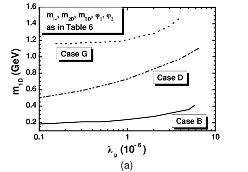
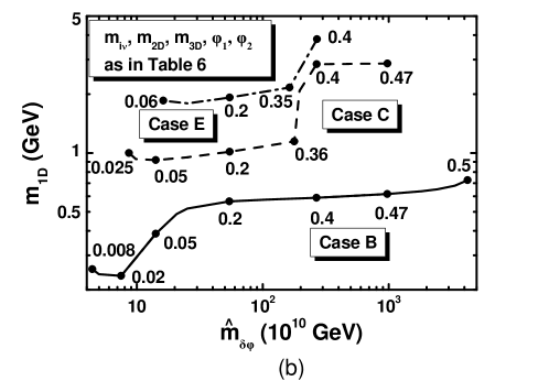
Figure 4: Contours, yielding the central $Y_{B}$ in Eq. (50) consistently with the inflationary requirements, in the (a) $\lambda_{\mu}-m_{\rm 1D}$ plane for $(n,r_{\pm})=(0.042,0.025)$; (b) $\widehat{m}_{\delta\phi}-m_{\rm 1D}$ plane for $n=0$ and $r_{\pm}$ values indicated on the curves. We also take $K=K_{2}$ or $K_{3}$ with ${N_{X}}=2$, $y=0.5$ and the values of $m_{i\nu}$, $m_{\rm 2D}$, $m_{\rm 3D}$, $\varphi_{1}$, and $\varphi_{2}$ which correspond to the cases B (solid line), C (dashed line), D (double dot-dashed line), E (dot-dashed line), and G (dotted line) of Table 6.

In order to investigate the robustness of the conclusions inferred from Table 6, we examine also how the central value of $Y_{B}$ in Eq. (50) can be achieved by varying $m_{\rm 1D}$ as a function of $\lambda_{\mu}$ and $\widehat{m}_{\rm\delta\phi}$ in Fig. 4-(a) and (b) respectively. Since the range of $Y_{B}$ in Eq. (50) is very narrow, the $95\%$ c.l. width of these contours is negligible. The convention adopted for these lines is also described in each plot. In particular, we use solid, dashed, dot-dashed, double dot-dashed and dotted line when the inputs – i.e. $m_{[\nu}i]$, $m_{[\rm D}2]$, $m_{[\rm D}3]$, $\varphi_{1}$, and $\varphi_{2}$ – correspond to the cases B, C, E, D, and G of Table 6, respectively. In both graphs we employ $K=K_{2}$ or $K_{3}$ with $N_{X}=2$ and $y=0.5$.

In Fig. 4-(a) we fix $(n,r_{\pm})$ to the value used in Table 6. Increasing $\lambda_{\mu}$ above its value shown in Table 6 the ratio $\widehat{\Gamma}_{\delta\phi\rightarrow N_{i}^{c}N_{i}^{c}}/\widehat{\Gamma}_{\rm\delta\phi}$ gets lower and an increase of $M_{[N^{c}}1]$ – and consequently on $m_{[\rm D}1]$ – is required to keep $Y_{B}$ at an acceptable level. As a byproduct, $T_{\rm rh}$ and $Y_{3/2}$ increase too and jeopardize the fulfillment of Eq. (52). Actually, along the depicted contours in Fig. 4-(a), we obtain $0.04\leq T_{\rm rh}/10^{8}~{}{\mbox{\rm GeV}}\leq 1.5$ whereas the resulting $M_{[N^{c}}1]$’s [$M_{[N^{c}}2]$’s] vary in the ranges $(0.8-3)\cdot 10^{10}~{}{\mbox{\rm GeV}}$, $(0.4-2)\cdot 10^{10}~{}{\mbox{\rm GeV}}$ and $(2.9-3.1)\cdot 10^{10}~{}{\mbox{\rm GeV}}$, [$(4-6)\cdot 10^{10}~{}{\mbox{\rm GeV}}$, $1.3\cdot 10^{12}~{}{\mbox{\rm GeV}}$ and $(3-4)\cdot 10^{10}~{}{\mbox{\rm GeV}}$] for the inputs of cases B, D and G respectively. Finally, $M_{[N^{c}}3]$ remains close to its values presented in the corresponding cases of Table 6. At the upper [lower] termination points of the contours, we obtain $Y_{B}$ lower [upper] that the value in Eq. (50).

In Fig. 4-(b) we fix $n=0$ and vary $r_{\pm}$ in the allowed range indicated in Fig. 2-(a). Only some segments from that range fulfill the post-inflationary requirements, despite the fact that the Majorana phases in Table 6 are selected so as to maximize somehow the relevant $\widehat{m}_{\rm\delta\phi}$ margin. Namely, as inferred by the numbers indicated on the curves in the $\widehat{m}_{\rm\delta\phi}-m_{[\rm D}1]$ plane, we find that $r_{\pm}$ may vary in the ranges $(0.008-0.499)$, $(0.025-0.47)$ and $(0.06-0.4)$ for the inputs of cases B, C and E respectively. The lower limit on these curves comes from the fact that $Y_{B}$ is larger than the expectations in Eq. (50). At the other end, Eq. (49b) is violated and, therefore, washout effects start becoming significant. At these upper termination points of the contours, we obtain $T_{\rm rh}$ of the order $10^{9}~{}{\mbox{\rm GeV}}$ or $Y_{3/2}>10^{-13}$ and so, we expect that the constraint of Eq. (52) will cut any possible extension of the curves beyond these termination points that could survive the possible washout of $Y_{L}$. As induced by Eqs. (41) and (42), $\widehat{m}_{\rm\delta\phi}$ increases with $r_{\pm}$ and so, an enhancement of $M_{[N^{c}}1]$’s and similarly of $m_{[\rm D}1]$’s is required so that $Y_{B}$ meets Eq. (50). The enhancement of $m_{[\rm D}1]$ becomes sharp until the point at which the decay channel of $\widehat{\delta\phi}$ into $N_{2}^{c}$’s rendered kinematically allowed.

Compared to the findings of the same analysis in other inflationary settings [6, 25, 26], the present scenario is advantageous since $\widehat{m}_{\rm\delta\phi}$ is allowed to reach lower values. Recall – see Sec. 5.1 – that the constant value of $\widehat{m}_{\rm\delta\phi}$ obtained in the papers above represents here the upper bound of $\widehat{m}_{\rm\delta\phi}$ which is approached when $r_{\pm}$ tends to its maximal value in Eq. (15). In practice, this fact offers us the flexibility to reduce $T_{\rm rh}$ and $Y_{3/2}$ at a level compatible with $m_{3/2}$ values as light as $1~{}{\mbox{\rm TeV}}$ which are excluded elsewhere. On the other hand, $Y_{B}$ increases when $\widehat{m}_{\rm\delta\phi}$ decreases and can be kept in accordance with the expectations due to variation of $m_{[\rm D}i]$ and $M_{[N^{c}}i]$. As a bottom line, nTL not only is a realistic possibility within our models but also it can be comfortably reconciled with the $\widetilde{G}$ constraint.

6 Conclusions

We investigated the realization of kinetically modified non-minimal HI (i.e. Higgs Inflation) and nTL (i.e. non-thermal leptogenesis) in the framework of a model which emerges from MSSM if we extend its gauge symmetry by a factor $U(1)_{B-L}$ and assume that this symmetry is spontaneously broken at a GUT scale determined by the running of the three gauge coupling constants. The model is tied to the super- and Kähler potentials given in Eqs. (3b) and (4a) – (4c). Prominent in this setting is the role of a softly broken shift-symmetry whose violation is parameterized by the quantity $r_{\pm}=c_{+}/c_{-}$. Combined variation of $r_{\pm}$ and $n$ – defined in Eq. (10) – in the ranges of Eq. (33) assists in fitting excellently the present observational data and obtain $r$’s which may be tested in the near future. Moreover, within our model, the $\mu$ problem of the MSSM is resolved via a coupling of the stabilizer field ($S$) to the electroweak higgses, provided that the relevant coupling constant, $\lambda_{\mu}$, is relatively suppressed. It is gratifying that the derived relation between $\mu$ and $m_{3/2}$ is compatible with successful low energy phenomenology of CMSSM. During the reheating phase that follows HI, the inflaton can decay into $N^{c}_{i}$’s (i.e., right-handed neutrinos) allowing, thereby for nTL to occur via the subsequent decay of $N^{c}_{i}$’s. Although other decay channels to the MSSM particles via non-renormalizable interactions are also activated, we showed that the generation of the correct $Y_{B}$, required by the observations BAU, can be reconciled with the inflationary constraints, the neutrino oscillation parameters and the $\widetilde{G}$ abundance, for masses of the (unstable) $\widetilde{G}$ as light as $1~{}{\mbox{\rm TeV}}$. More specifically, we found that only $N_{1}^{c}$ and $N_{2}^{c}$ with masses lower than $1.8\cdot 10^{13}~{}{\mbox{\rm GeV}}$ can be produced by the inflaton decay which leads to a reheating temperature $T_{\rm rh}$ as low as $2.7\cdot 10^{7}~{}{\mbox{\rm GeV}}$.

References

- [1]
- [2]
-
[3]
A.H. Guth, Phys. Rev. D231981347;
A.D. Linde, Phys. Lett. B 108, 389 (1982);
A. Albrecht and P.J. Steinhardt, Phys. Rev. Lett. 48, 1220 (1982). -
[4]
D.S. Salopek, J.R. Bond and J.M. Bardeen, Phys.
Rev. D 40, 1753 (1989);
J.L. Cervantes-Cota and H. Dehnen, Phys. Rev. D511995395 [\astroph9412032]. -
[5]
G.R. Dvali, Q. Shafi and R.K. Schaefer, Phys. Rev. Lett.7319941886 [hep-ph/9406319];
L. Covi et al., \plb4241998253 [\hepph9707405];
B. Kyae and Q. Shafi, Phys. Rev. D722005063515 [\hepph0504044];
B. Kyae and Q. Shafi, \plb6352006247 [\hepph0510105];
R. Jeannerot, S. Khalil and G. Lazarides, \jhep072002069 [hep-ph/0207244];
W. Buchmüller, V. Domcke and K. Schmitz, \npb8622012587 [\arxiv1202.6679]. -
[6]
C. Pallis
and N. Toumbas, J. Cosmology Astropart. Phys122011002 [\arxiv1108.1771];
C. Pallis and N. Toumbas, “Open Questions in Cosmology” (InTech, 2012) [\arxiv1207.3730]. -
[7]
S. Antusch et al.,
\jhep082010100 [\arxiv1003.3233];
K. Nakayama and F. Takahashi, J. Cosmology Astropart. Phys052012035 [\arxiv1203.0323];
M.B. Einhorn and D.R.T. Jones, J. Cosmology Astropart. Phys112012049 [\arxiv1207.1710];
L. Heurtier, S. Khalil and A. Moursy, J. Cosmology Astropart. Phys102015045 [\arxiv1505.07366];
G.K. Leontaris, N. Okada and Q. Shafi, \plb7652017256 [\arxiv1611.10196]. -
[8]
M. Arai, S. Kawai and N. Okada, Phys. Rev. D
84,1 23515 (2011) [\arxiv1107.4767];
J. Ellis, H.J. He and Z.Z. Xianyu, Phys. Rev. D 91, no. 2, 021302 (2015) [\arxiv1411.5537];
J. Ellis, H.J. He and Z.Z. Xianyu, J. Cosmol. Astropart. Phys. 08, no. 08, 068 (2016) [\arxiv1606.02202];
S. Kawai and J. Kim, Phys. Rev. D 93, no. 6, 065023 (2016) [\arxiv1512.05861]. -
[9]
J. Ellis et al., J. Cosmol. Astropart.
Phys. 11, no. 11, 018 (2016) [\arxiv1609.05849];
J. Ellis et al., J. Cosmol. Astropart. Phys. 07, no. 07, 006 (2017) [\arxiv1704.07331]. - [10] C. Pallis, Phys. Rev. D 92, no. 12, 121305(R) (2015) [\arxiv1511.01456].
- [11] C. Pallis, J. Cosmol. Astropart. Phys. 10, no. 10, 037 (2016) [\arxiv1606.09607].
-
[12]
C. Pallis, Phys. Rev. D 91, no. 12, 123508 (2015) [\arxiv1503.05887];
C. Pallis, PoS PLANCK 2015, 095 (2015) [\arxiv1510.02306]. -
[13]
F. Takahashi, Phys. Lett. B
693, 140 (2010) [\arxiv1006.2801];
K. Nakayama and F. Takahashi, J. Cosmology Astropart. Phys112010009 [\arxiv1008.2956];
H.M. Lee, Eur. Phys. J. C 74, 3022 (2014) [\arxiv1403.5602]. - [14] C. Pallis, \plb6922010287 [\arxiv1002.4765].
- [15] R. Kallosh, A. Linde and D. Roest, Phys. Rev. Lett. 112, 011303 (2014) [\arxiv1310.3950].
- [16] P.A.R. Ade et al. [Planck Collaboration], Astron. Astrophys. 594, A20 (2016) [\arxiv1502.02114].
-
[17]
P.A.R. Ade et al. [BICEP2/Keck Array
Collaborations],
Phys. Rev. Lett. 116, 031302 (2016) [\arxiv1510.09217]. -
[18]
J.L.F. Barbon and J.R. Espinosa,
Phys. Rev. D792009081302 [\arxiv0903.0355];
C.P. Burgess, H.M. Lee, and M. Trott, \jhep072010007 [\arxiv1002.2730]. - [19] A. Kehagias, A.M. Dizgah and A. Riotto, Phys. Rev. D892014043527 [\arxiv1312.1155].
-
[20]
M. Kawasaki, M. Yamaguchi and T. Yanagida,
Phys. Rev. Lett.8520003572 [\hepph0004243];
P. Brax and J. Martin, Phys. Rev. D 72, 023518 (2005) [\hepth0504168];
S. Antusch, K. Dutta and P.M. Kostka, \plb6772009221 [\arxiv0902.2934];
R. Kallosh, A. Linde and T. Rube, Phys. Rev. D832011043507 [\arxiv1011.5945];
T. Li, Z. Li and D.V. Nanopoulos, J. Cosmology Astropart. Phys022014028 [\arxiv1311.6770];
K. Harigaya and T.T. Yanagida, \plb734201413 [\arxiv1403.4729];
A. Mazumdar, T. Noumi and M. Yamaguchi, Phys. Rev. D902014043519 [\arxiv1405.3959];
C. Pallis and Q. Shafi, \plb7362014261 [\arxiv1405.7645]. - [21] I. Ben-Dayan and M.B. Einhorn, J. Cosmology Astropart. Phys122010002 [\arxiv1009.2276].
- [22] G. Lazarides and C. Pallis, J. High Energy Phys. 11, 114 (2015) [\arxiv1508.06682].
-
[23]
C. Pallis and N. Toumbas, J. Cosmology Astropart. Phys052016no. 05, 015
[\arxiv1512.05657];
C. Pallis and N. Toumbas, Adv. High Energy Phys. 2017, 6759267 (2017) [\arxiv1612.09202];
C. Pallis, PoS EPS-HEP 2017, 047 (2017) [\arxiv1710.04641]. -
[24]
K. Hamaguchi, Phd Thesis
[\hepph0212305];
W. Buchmüller, R.D. Peccei and T. Yanagida, Ann. Rev. Nucl. Part. Sci. 55, 311 (2005) [\hepph0502169]. - [25] C. Pallis, J. Cosmology Astropart. Phys042014024; 07, 01(E)(2017) [\arxiv1312.3623].
- [26] C. Pallis and Q. Shafi, Phys. Rev. D862012023523 [\arxiv1204.0252].
- [27] P.A.R. Ade et al. [Planck Collaboration], Astron. Astrophys. 594, A13 (2016) [\arxiv1502.01589].
-
[28]
G. Lazarides and Q. Shafi, \plb2581991305;
K. Kumekawa, T. Moroi and T. Yanagida, Prog. Theor. Phys. 92, 437 (1994) [\hepph9405337];
G. Lazarides, R.K. Schaefer and Q. Shafi, Phys. Rev. D5619971324 [hep-ph/9608256]. -
[29]
M.Yu. Khlopov and A.D. Linde,
Phys. Lett. B 138, 265 (1984);
J. Ellis, J.E. Kim, and D.V. Nanopoulos, \plb1451984181. -
[30]
M.Bolz, A.Brandenburg and W. Buchmüller,
Nucl. Phys. B606, 518 (2001); 790, 336(E)
(2008) [\hepph0012052];
J. Pradler and F.D. Steffen, Phys. Rev. D752007023509 [\hepph0608344]. -
[31]
R.H. Cyburt et al., Phys. Rev. D672003103521 [astro-ph/0211258];
M. Kawasaki, K. Kohri and T. Moroi, Phys. Lett. B 625, 7 (2005) [\astroph0402490];
M. Kawasaki, K. Kohri and T. Moroi, Phys. Rev. D712005083502 [\astroph0408426];
J.R. Ellis, K.A. Olive and E. Vangioni, \plb619200530 [\astroph0503023]. -
[32]
J. Ellis et al., J. Cosmol. Astropart.
Phys. 03, no. 03, 008 (2016) [\arxiv1512.05701];
Y. Ema et al., \jhep112016184 [\arxiv1609.04716]. - [33] D.V. Forero, M. Tortola and J.W.F. Valle, Phys. Rev. D 90, no. 9, 093006 (2014) [\arxiv1405.7540].
-
[34]
M.C. Gonzalez-Garcia, M. Maltoni and T. Schwetz, \jhep112014052 [\arxiv1409.5439];
F. Capozzi et al., Nucl. Phys. B 908, 218 (2016) [\arxiv1601.07777].‘ - [35] G.R. Dvali, G. Lazarides and Q. Shafi, Phys. Lett. B 424, 259 (1998) [\hepph9710314].
- [36] M. Endo, F. Takahashi and T.T. Yanagida, Phys. Rev. D762007083509 [arXiv:0706.0986].
-
[37]
M.B. Einhorn and D.R.T. Jones,
\jhep032010026 [\arxiv0912.2718];
H.M. Lee, J. Cosmology Astropart. Phys082010003 [\arxiv1005.2735];
S. Ferrara et al., Phys. Rev. D832011025008 [\arxiv1008.2942];
C. Pallis and N. Toumbas, J. Cosmology Astropart. Phys022011019 [\arxiv1101.0325]. -
[38]
G. Lopes Cardoso, D. Lüst and T. Mohaupt, Nucl. Phys.
B432 68 (1994) [\hepth9405002];
I. Antoniadis, E. Gava, K.S. Narain and T.R. Taylor, Nucl. Phys. B432 187 (1994) [\hepth9405024]. -
[39]
C. Pallis, J. Cosmology Astropart. Phys102014058
[\arxiv1407.8522];
C. Pallis and Q. Shafi, J. Cosmology Astropart. Phys032015no. 03, 023 [\arxiv1412.3757];
C. Pallis, PoS CORFU 2014, 156 (2015) [\arxiv1506.03731]. -
[40]
R. Kallosh, A. Linde and D. Roest,
\jhep112013198 [\arxiv1311.0472];
R. Kallosh, A. Linde and D. Roest, \jhep082014052 [\arxiv1405.3646]. - [41] L. Boubekeur and D. Lyth, J. Cosmol. Astropart. Phys. 07, 010 (2005) [\hepph0502047].
-
[42]
R.Armillis and C.Pallis,“Recent Advances in
Cosmology” (Nova Science Publishers, 2012) [\arxiv1211.4011];
B. Garbrecht, C. Pallis and A. Pilaftsis, \jhep122006038 [\hepph0605264];
C. Pallis and Q. Shafi, Phys. Lett. B 725, 327 (2013) [\arxiv1304.5202];
M. Civiletti, C. Pallis and Q. Shafi, Phys. Lett. B 733, 276 (2014) [\arxiv1402.6254]. - [43] S. Antusch and M. Spinrath, Phys. Rev. D 78, 075020 (2008) [\arxiv0804.0717].
- [44] S.R. Coleman and E.J. Weinberg, Phys. Rev. D719731888.
-
[45]
D.H. Lyth and
A. Riotto, Phys. Rept. 314, 1 (1999) [hep-ph/9807278];
G. Lazarides, J. Phys. Conf. Ser. 53, 528 (2006) [hep-ph/0607032];
J. Martin, C. Ringeval and V. Vennin, Physics of the Dark Universe 5-6, 75 (2014) [\arxiv1303.3787]. - [46] http://functions.wolfram.com.
- [47] W.L.K. Wu et al., J. Low. Temp. Phys. 184, no. 3-4, 765 (2016) [\arxiv1601.00125].
- [48] P. Andre et al. [PRISM Collaboration], \arxiv1306.2259.
- [49] T. Matsumura et al., J. Low. Temp. Phys. 176, 733 (2014) [\arxiv1311.2847].
- [50] S.P. Martin, Adv. Ser. Direct. High Energy Phys. 21, 1 (2010) [\hepph9709356].
- [51] P. Athron et al. [GAMBIT Collaboration], Eur. Phys. J. C 77, no. 12, 824 (2017) [\arxiv1705.07935].
-
[52]
W. Buchmüller et al., \jhep092014053
[\arxiv1407.0253];
J. Ellis, M. Garcia, D. Nanopoulos and K. Olive, J. Cosmology Astropart. Phys102015003 [\arxiv1503.08867]. - [53] H.P. Nilles, Phys. Rept. 110, 1 (1984).
- [54] C. Pallis, \npb7512006129 [\hepph0510234].
- [55] V.N. Şenoğuz, Phys. Rev. D762007013005 [arXiv:0704.3048].
-
[56]
J.L. Feng, A. Rajaraman and F. Takayama, Phys. Rev. D682003063504
[\hepph0306024];
F.D. Steffen, J. Cosmology Astropart. Phys092006001 [\hepph0605306];
T. Kanzaki, M. Kawasaki, K. Kohri and T. Moroi, Phys. Rev. D752007025011 [\hepph0609246];
L. Roszkowski et al., \jhep032013013 [\arxiv1212.5587]. -
[57]
M. Dine, R. Kitano, A. Morisse and Y. Shirman, Phys. Rev. D732006123518 [\hepph0604140];
R. Kitano, \plb6412006203 [\hepph0607090];
J.L. Evans, M.A.G. Garcia and K.A. Olive, J. Cosmology Astropart. Phys032014022 [\arxiv1311.0052]. -
[58]
M. Flanz, E.A. Paschos and U. Sarkar,
Phys. Lett. B 345, 248 (1995); 382, 447(E)
(1996) [\hepph9411366];
L. Covi, E. Roulet and F. Vissani, \plb3841996169 [\hepph9605319];
M. Flanz, E.A. Paschos, U. Sarkar and J. Weiss, \plb3891996693 [\hepph9607310]. - [59] R. Armillis, G. Lazarides and C. Pallis, Phys. Rev. D 89, 065032 (2014) [\arxiv1309.6986].
- [60] S. Antusch, J. Kersten, M. Lindner and M. Ratz, \npb6742003401 [\hepph0305273].
- [61] G. Lazarides and Q. Shafi, Phys. Rev. D 58, 071702 (1998) [\hepph9803397].
- [62] N. Karagiannakis, G. Lazarides and C. Pallis, Int. J. Mod. Phys. A 28, 1330048 (2013) [\arxiv1305.2574].