A Comparison of Testing Methods in Scalar-on-Function Regression

Supplementary Material for “A Comparison of Testing Methods in Scalar-on-Function Regression”

Abstract

A scalar-response functional model describes the association between a scalar response and a set of functional covariates. An important problem in the functional data literature is to test the nullity or linearity of the effect of the functional covariate in the context of scalar-on-function regression. This article provides an overview of the existing methods for testing both the null hypotheses that there is no relationship and that there is a linear relationship between the functional covariate and scalar response, and a comprehensive numerical comparison of their performance. The methods are compared for a variety of realistic scenarios: when the functional covariate is observed at dense or sparse grids and measurements include noise or not. Finally, the methods are illustrated on the Tecator data set.

1 Introduction

The scalar-on-function regression model refers to the situation where the response variable is a scalar, and the predictor variable is functional. Such models are generalizations of the usual regression models with a vector-valued covariate, both linear and nonlinear, to the case with functional covariates. The functional version of standard linear regression is the so-called functional linear model (FLM)(see, e.g., Ramsay and Dalzell [1991]); various extensions to nonparametric functional regression models have also been developed (see, e.g., Ferraty and Vieu [2006]). In this article, we are concerned with hypothesis testing procedures in such scalar-on-function regression models. As in standard regression models, one important problem is to test whether there is any association between the functional covariate and the response, that is, the test for nullity. Also, for nonparametric or nonlinear functional regression models, another equally important question is to test linearity of the relationship between the functional covariate and the scalar response; this is primarily because of the interpretability and ease of fit of the FLM. There is a plethora of literature that develops statistical methods for testing nullity and linearity in both linear and nonlinear scalar-on-function regression models, respectively. Despite the various available methods, there is no clear guideline as to which method provides the best performance in different situations. In this article, our goal is to provide an overview of the available testing methods, perform an extensive numerical study to compare their size and power performance in various data generation models and provide a guideline as to which method yields to the best performance. We will illustrate the discussed methods via the Tecator data set.

Much of the literature on testing nullity has been developed under the assumption that there is a linear relationship between the functional covariate and the scalar response, that is, the functional linear model (FLM). First introduced by Ramsay and Dalzell [1991], the FLM is one of the most commonly used functional regression models due to its interpretability and simplicity. It has received extensive attention in recent literature; see Ramsay and Silverman [1997, 2005], Cardot et al. [1999], Müller and Stadtmüller [2005], Ferraty and Vieu [2006], Cai et al. [2006], Hall et al. [2007], Crambes et al. [2009], and Goldsmith et al. [2011]. The FLM quantifies the effect of the functional covariate as an integral of the functional covariate weighted by an unknown coefficient function. The test for nullity, in this case, involves testing whether the coefficient function is zero or not.

Cardot et al. [2003] proposed two testing methods that are based on the norm of the cross-covariance operator of the functional covariate and the scalar response for testing nullity in the FLM. They provided asymptotic normality and consistency results of the two proposed test statistics. Later, Cardot et al. [2004] considered an alternative approach based on a direct approximation of the distribution of the cross-covariance operator. Furthermore, they proposed a pseudo-likelihood test statistic for the situation when there are multiple functional predictors. Assuming an FLM, Swihart et al. [2014] proposed likelihood ratio-based test statistics, representing the model by using a mixed-effects modeling framework and rewriting the null hypothesis with zero-variance components. The major advantage of the mixed-effects model is that software is readily available for estimation and hypothesis testing. Recently, Kong et al. [2016] considered traditional testing methods—Wald, score, likelihood ratio, and F, to test for no effect in the FLM. They derived the theoretical properties of each testing method and compared their performances for both densely and sparsely sampled functions.

The main disadvantage of the FLM is the assumption of linearity of the relationship between the functional covariate and the scalar response. Such a linear relationship may not be practical in many situations, and as a result, there is a substantial amount of literature on the development of nonlinear/nonparametric functional regression models. Yao and Müller [2010] considered a quadratic regression model as an extension of the FLM by including quadratic effects of the functional covariate. García-Portugués et al. [2014] considered testing in a nonparametric functional regression model, where the effect of the functional covariate was modeled via an unknown functional. McLean et al. [2014] developed the so-called functional generalized additive model (FGAM), where the effect of the functional covariate is modeled using an integral of a bivariate smooth function involving the functional covariate at a specific time point and the time point itself. For testing nullity, García-Portugués et al. [2014] introduced the projected Cramér-von Mises (PcVM) test—a testing method which is derived by using random projection, and whose null distribution is approximated by bootstrap. McLean et al. [2015] introduced a restricted likelihood ratio test (RLRT) statistic for testing no effect under the assumption that the response and the predictor are related through an FGAM. The key idea is to use the mixed model formulation of the smooth effects and represent the null hypothesis as the test for a subset of variance components.

Other than testing for nullity, another important problem is to test for linearity of the regression function. Motivated by the idea of a polynomial functional relationship (e.g., quadratic functional regression by Yao and Müller [2010]), Horváth and Reeder [2013] developed a testing method by using functional principal component scores to test the null effect of the quadratic term and studied its asymptotic properties. The testing methods of García-Portugués et al. [2014] and McLean et al. [2015] can also be used to investigate the problem of testing for the linear effect.

In this article, our goal is to numerically compare the performance of all the existing methods for testing nullity as well as linearity of a functional covariate when the response is scalar in a variety of scenarios related to how the functional covariate is observed. The results are illustrated for varying sample sizes and situations of increasing complexity regarding the functional covariate. Additionally, we apply the methods to a commonly used data set, the Tecator data, to formally assess the relationship between the meat’s spectrum of absorbances and the fat content, using 215 finely chopped pure meat samples.

The article makes two key contributions to the literature. First, we study each of these methods under a wide variety of scenarios in which the functional predictor is observed either on a dense or sparse grid of points for each subject, with or without measurement error. Much of the previous work relies only on the assumption of densely observed functional predictors. Second, we provide a comprehensive comparison study of the existing approaches for testing nullity and linearity of scalar-on-function regression.

The remainder of the article is organized as follows. In Section 2, we introduce the data structure and model framework for scalar-on-function regression. In Section 3, we review each of the methods under comparison. Section 4 discusses the advantages and drawbacks of each method in greater detail. Simulation studies and the real data application follow in Section 5 and 6, respectively.

2 Model Framework

Suppose that for subject $i\in\{1,\ldots,n\}$ we observe data of the form $\{Y_{i},(X_{ij},t_{ij}):j=1,\ldots,J\}$, where $Y_{i}$ is a scalar response variable and $X_{ij}=X_{i}(t_{ij})$ are discrete realizations of a real-valued, square-integrable smooth curve $X_{i}(\cdot)$ at observation points $t_{ij}$. For simplicity of exposition, we assume that the full predictor trajectory $X_{i}(\cdot)$ is observed; however, the methods are investigated for the case when the true predictor is observed on a finite grid of points and corrupted with measurement error. Without loss of generality, we assume that the functional covariate is a zero-mean process. A scalar-response functional model can be defined as

$$Y_{i}=\alpha+m\{X_{i}(\cdot)\}+\varepsilon_{i},$$ (1)

where $m(\cdot)$ is an unknown functional and $\varepsilon_{i}$ are independent and identically distributed random errors with mean zero and variance $\sigma^{2}$. According to Ferraty and Vieu [2006], $m(\cdot)$ can be classified as parametric and nonparametric, depending on the specific mean model at hand. An example of a functional parametric mean model is the functional linear model (FLM) where $m\{X_{i}(\cdot)\}=\int X_{i}(t)\beta(t)dt$ for some unknown continuous function $\beta(\cdot)$. In contrast, a functional nonparametric mean model assumes that the object $m(\cdot)$ is a continuous real-valued operator defined on a Hilbert space $\mathbb{H}$. In this article, we are interested in testing two important hypotheses about the mean structure: (i) $H_{01}:m\{X(\cdot)\}=\int X(t)\beta(t)dt$, the relationship between the covariate $X(\cdot)$ and the response $Y$ is linear, and (ii) $H_{02}:m\{X(\cdot)\}=0\;\text{for any}\;t\in\mathcal{T}$, there is no relationship between $X(\cdot)$ and $Y$.

The main focus of this article is to numerically compare the performance of the existing methods for testing $H_{01}$ and $H_{02}$ in a variety of realistic scenarios. For testing $H_{01}$, we study the nonparametric testing method of García-Portugués et al. [2014] (which we call GGF using first letters of the authors’ names), the semi-parametric method of McLean et al. [2015] (which we call MHR), and the parametric method of Horváth and Reeder [2013] (which we call HR). For testing $H_{02}$, we study the GGF and MHR methods, and also the parametric method of Kong et al. [2016] (referred by KSM), which assumes a linear relationship between the response and the predictor. We assess the performance of the methods in the cases when the functional covariate is observed on a dense, moderately sparse, or sparse grid, with and without measurement error, using different sample sizes. This article offers a comprehensive comparison study of available approaches in the literature for testing nullity and linearity in scalar-on-function regression.

3 Hypothesis Testing

In this section, we review each of the methods under study. All the methods rely on the idea of using basis expansion to approximate the functional linear model by a simple mixed-effects model. The various methods use different test statistics and corresponding null distributions, and they have been developed to assess the null hypothesis in specific settings. First, we consider the problem of testing linearity. The GGF method considers this problem in the class of nonlinear models, which is the most general case considered in the literature. In contrast, MHR and HR consider this problem in a more restrictive class of models: MHR assumes a functional generalized additive model (FGAM), and HR assumes a functional quadratic model. For testing nullity, GGF assumes a general non-null relationship, MHR assumes an FGAM relationship, and KSM assumes a linear dependence. These assumptions are reflected in the form of the alternative hypothesis. The HR and KSM methods are parametric methods that require stronger assumptions in order to develop their corresponding null distributions.

3.1 Testing for the Linear Effect of the Functional Covariate

3.1.1 GGF Method for Testing Linearity $H_{01}$

The GGF method [García-Portugués et al., 2014] for testing linearity is essentially a generalization of a goodness-of-fit test in regression models for scalar responses and vector covariates to the case when the covariate is functional. The interest is to test the null hypothesis $H_{01}$, which indicates that $m(\cdot)$ belongs to the family $\mathcal{M}=\{\langle\cdot,\beta\rangle:\beta\in\mathbb{H}=L^{2}[0,1]\}$ versus a general alternative of the form $H_{A1}:m\notin\{\langle\cdot,\beta\rangle:\beta\in\mathbb{H}\}$ with positive probability. In other words, the alternative hypothesis can also be written as

$$H_{A1}:E(Y)=m\{X(\cdot)\},$$ (2)

where $m(\cdot)$ is an unknown functional, while the null hypothesis is that $m\{X(\cdot)\}=\langle X(\cdot),\beta\rangle$.

The key idea is to characterize the linear relationship in an equivalent way that is based on random projection. Specifically, García-Portugués et al. [2014] show that $m\{X(\cdot)\}=\langle X(\cdot),\beta\rangle$ for $\beta$ an element in $L^{2}[0,1]$ is equivalent to

$$E[(Y-\langle X(\cdot),\beta\rangle)\mathds{1}_{\{\langle X(\cdot),\gamma\rangle\leq u\}}]=0,$$ (3)

almost everywhere for any $u\in\mathbb{R}$ and for all $\gamma\in\mathbb{S}_{\mathbb{H}}^{p},\forall p\geq 1$, where $\mathbb{S}^{p}_{\mathbb{H}}=\{f=\sum_{j=1}^{p}x_{j}\Psi_{j}\in\mathbb{H}:||f||_{\mathbb{H}}=1\}$ and $f:[0,1]\rightarrow\mathbb{R}$ such that their norm $||f||_{\mathbb{H}}=(\int_{0}^{1}|f(t)|^{2}dt)^{1/2}$, and $\{\Psi_{1}(\cdot),\Psi_{2}(\cdot),\ldots\Psi_{p}(\cdot)\}$ are orthogonal bases in $L^{2}[0,1]$. For more information, see Lemma 3.1 in García-Portugués et al. [2014]. The latter formulation essentially implies that the mean of the departure from a linear relationship—that is, concentrated on arbitrarily small neighborhoods, is zero. Thus, one approach to testing for linearity is to quantify the mean on the left-hand side of (3) and assess how different it is from zero.

The GGF method proposes to do this by first estimating $\beta(\cdot)$ by the best linear estimator, $\hat{\beta}(\cdot)$, using known basis functions to expand both the functional covariate and the coefficients, and then rewriting the functional linear model as a standard linear model, as proposed by Cardot et al. [1999]. The residuals under the null hypothesis are $\hat{\varepsilon_{i}}=Y_{i}-\hat{Y}_{i}=Y_{i}-\int X_{i}(t)\hat{\beta}(t)dt\;\text{for}\;i=1,\ldots,n$. Once the residuals are estimated, a projected Cramér-von Mises (PcVM) test statistic with a plug-in estimator is used. Specifically, for fixed $u$ and $\gamma\in\mathbb{S}_{\mathbb{H}}$, a method of moment estimator of (3) is $n^{-1/2}\hat{R}_{n}(u,\gamma)$, where

$$\hat{R}_{n}(u,\gamma)=n^{-1/2}\sum_{i=1}^{n}\hat{\varepsilon_{i}}\mathds{1}_{\int X_{i}(t)\gamma(t)dt\leq u}.$$ (4)

The PcVM test statistic is adapted to the projected space $\Pi=\mathbb{R}\times\mathbb{S}_{L^{2}[0,1]}$ and defined as

$$\text{PCvM}_{n,p}=\int_{\Pi}\hat{R}_{n}(u,\gamma)^{2}F_{n,\gamma}(du)\omega(d\gamma),$$ (5)

where $F_{n,\gamma}$ is the empirical cumulative distribution function of the data $\{\langle X_{i}(\cdot),\gamma\rangle\}_{i=1}^{n}$ and $\omega$ is a measure on $\mathbb{S}_{\mathbb{H}}$.

This expression is certainly complicated, and its derivation has numerous cumbersome steps. However, García-Portugués et al. [2014] show that in practice $\mbox{PCvM}_{n,p}$ is approximated by $n^{-2}\hat{\varepsilon}^{T}\boldsymbol{A}\hat{\varepsilon}$, where $\boldsymbol{A}=(\sum_{r=1}^{n}A_{ijr})_{ij}$ is an $n\times n$ matrix of the average over $i$ and $j$ of the three-dimensional array $A_{ijr}$. The array represents the product surface area of a spherical wedge of angle $A_{ijr}^{(0)}$ times the determinant of the matrix $R^{-1}$ (from the Cholesky decomposition of the basis functions). For details concerning the matrix $\boldsymbol{A}$ and the derivation of this approximation, we refer the reader to García-Portugués et al. [2014]. The null distribution of the test statistic is nonstandard and is approximated by a wild bootstrap on the residuals.

3.1.2 MHR Method for Testing Linearity $H_{01}$

The MHR method [McLean et al., 2015] considers testing in the class of models called functional generalized additive model (FGAM), for which the response and covariate relate according to the following relationship:

$$Y=\alpha+\int_{\mathcal{T}}F\{X(t),t\}dt+\varepsilon;$$ (6)

we use the generic notation $\{Y,X(\cdot),\varepsilon\}$ respectively for the response, functional covariate, and Gaussian random error with zero mean and variance $\sigma^{2}$, and $F(\cdot,\cdot)$ represents an unknown bivariate function. It can be clearly seen that FGAM reduces to the FLM when $F(x,t)=x\beta(t)$; thus FLM is a special class of FGAM. Testing the hypothesis of interest in this class is equivalent to representing the alternative hypothesis as $H_{A1}:E(Y)=\alpha+\int_{\mathcal{T}}F\{X(t),t\}dt$. The key idea behind the test is to use the connection between the tensor product splines and mixed-effects modeling [Wood et al., 2013] and to formulate the FGAM as a mixed model representation with two main parts: a component represented by unpenalized, fixed effects and a component represented by random effects.

Using low-rank spline bases, denoted as $\{B_{j}^{X}(x):j=1,\ldots,K_{x}\}$ and $\{B^{T}_{k}(t):k=1,\ldots,K_{t}\}$, the bivariate surface can be expanded as

$$F(x,t)=\sum_{j=1}^{K_{X}}\sum_{k=1}^{K_{t}}B_{j}^{X}(x)B_{k}^{T}(t)\theta_{jk},$$ (7)

where the $\theta_{jk}$ are unknown tensor product B-spline coefficients. Let $\mathbb{B}_{x}$ denote the $nJ\times K_{x}$ matrix of the $x$-axis B-splines that are evaluated at $\boldsymbol{x}=\mbox{vec}(\boldsymbol{X})$, where $\boldsymbol{X}=\{X_{i}(t_{im})\}$ is the $n\times J$ matrix whose rows include the observed functional predictor values for each subject. Similarly, let $\mathbb{B}_{t}$ denote the $nJ\times K_{t}$ matrix of the $t$-axis B-splines that are evaluated at $\boldsymbol{t}=\mbox{vec}(\boldsymbol{T})$, where $\boldsymbol{T}=\{t_{im}\}$ is the $n\times J$ matrix in which each row includes the observed time points for the functional predictor for each subject. The matrices $\mathbb{X}_{x}$, $\mathbb{Z}_{x}$, $\mathbb{X}_{t}$, and $\mathbb{Z}_{t}$ are derived from the eigendecompositions of marginal penalty matrices $\mathbb{P}_{x}$ and $\mathbb{P}_{t}$. After some mathematical manipulations, we can define the fixed-effects design matrix $\mathbb{X}=[\boldsymbol{1}:\boldsymbol{x}:\boldsymbol{x}\otimes\boldsymbol{t}]$, and the random-effects design matrices $\mathbb{Z}_{1}=\boldsymbol{x}\Box\mathbb{Z}_{t}$, $\mathbb{Z}_{2}=\mathbb{Z}_{x}\Box\mathbb{X}_{t}$, and $\mathbb{Z}_{3}=\mathbb{Z}_{x}\Box\mathbb{Z}_{t}$, where $\otimes$ denotes the Kronecker product and $\Box$ represents the box product (also known as the row-wise Kronecker product). Then, FGAM can be expressed in the form of a mixed-effects model with three pairwise independent vectors of random effects, each with a diagonal covariance matrix independent of the other effects:

$$\textbf{Y}\approx\mathbb{LX}\boldsymbol{\beta}+\sum_{j=1}^{3}\mathbb{LZ}_{j}\boldsymbol{b}_{j}+\boldsymbol{\varepsilon},$$ (8)

where $\mathbb{L}$ is an $n\times nJ$ matrix of quadrature weights; $\boldsymbol{b}_{j}\sim N(\boldsymbol{0},\sigma^{2}_{j}\mathbb{I}_{q_{j}})$ with the dimensions $q_{1}=K_{t}-2$, $q_{2}=2(K_{x}-2)$, and $q_{3}=(K_{x}-2)(K_{t}-2)$; and $\boldsymbol{\varepsilon}\sim N(\boldsymbol{0},\sigma^{2}_{e}\mathbb{I}_{N})$. The matrix $\mathbb{X}$ forms a basis for functions of the form $\beta_{0}+\beta_{1}x+\beta_{3}xt$ without penalty, $\mathbb{Z}_{1}$ forms a basis for functions of the form $xf_{2}(t)$ and penalty $\int(\partial_{tt}f_{2})^{2}$, $\mathbb{Z}_{2}$ forms a basis for functions of the form $g_{1}(x)+tg_{2}(x)$ and penalty $\int(\partial_{xx}g_{1})^{2}+\int(\partial_{xx}g_{2})^{2}$, and $\mathbb{Z}_{3}$ forms a basis for functions of the form $h(x,t)$ without the previous terms and with penalty $\int(\partial_{xxtt}h)^{2}$. In addition, it can be shown that the FLM is nested within the FGAM in an explicit way, which allows the use of restricted likelihood ratio tests for zero-variance components to test the null hypothesis that the functional linear model holds, $H_{01}:\sigma_{2}^{2}=\sigma_{3}^{2}=0$. The testing is done via the restricted likelihood ratio test (RLRT) under the assumption that $\sigma_{2}=\sigma_{3}$:

$$\text{RLRT}=2\sup_{H_{1}}\ell_{R}(\boldsymbol{y})-2\sup_{H_{0}}\ell_{R}(\boldsymbol{y}),$$

where $\ell_{R}$ denotes the restricted log-likelihood function of the observed data vector $\boldsymbol{y}$ for model (8). Crainiceanu and Ruppert [2004] derive the finite-sample null distribution of the RLRT statistic and show that the distribution is different from the mixture of $\chi^{2}$ distributions.

3.1.3 HR Method for Testing Linearity $H_{01}$

The HR method [Horváth and Reeder, 2013] considers the same problem and proposes a method based on projecting the predictor process onto a space of finite dimension by using the functional principal component analysis (FPCA). This approach assumes a functional quadratic regression model

$$Y=\alpha+\int X(t)\beta(t)dt+\iint X(t)X(s)\gamma(s,t)dtds+\varepsilon,$$ (9)

where $\beta(t)$ and $\gamma(s,t)$ are unknown smooth univariate and bivariate functions, respectively. Notice that when $\gamma(s,t)=0$, model (9) reduces to the FLM; equivalently the FLM is a subclass of model (9). Horváth and Reeder [2013] focus on testing the significance of the quadratic term in model (9); that is, they focus on the null hypothesis $H_{01}:\gamma(s,t)=0$ versus $H_{A1}:\gamma(s,t)\neq 0$.

The regression coefficient functions are expanded using the eigenfunctions of the covariance function of the predictor $C(t,s)=E\{X_{i}(t)-\mu_{x}(t)\}\{X_{i}(s)-\mu_{X}(s)\}$ to represent them as $\beta(t)=\sum_{j=1}^{p}b_{j}v_{j}(t)$ and $\gamma(s,t)=\sum_{j=1}^{p}\sum_{k=1}^{p}a_{jk}v_{k}(s)v_{j}(t)$, where $v_{j}(t)$ denote the eigenfunctions of $C(t,s)$. By projecting the observations onto the space spanned by $\{v_{j}(t)\}_{j=1}^{p}$ and using the expansions given above, we can rewrite model (9) as

$$Y_{i}=\alpha+\sum_{j=1}^{p}b_{j}\langle X_{i},v_{j}\rangle+\sum_{j=1}^{p}\sum_{k=1}^{p}\{2-\mathds{1}(j=k)\}a_{jk}\langle X_{i},v_{j}\rangle\langle X_{i},v_{k}\rangle+\varepsilon_{i}^{*},$$ (10)

where $a_{jk}$ and $b_{j}$ are the coefficients, and

$$\varepsilon_{i}^{*} =\varepsilon_{i}+\sum_{j=p+1}^{\infty}b_{j}\langle X_{i},v_{j}\rangle+\sum_{j=p+1}^{\infty}\sum_{k=j}^{\infty}\{2-\mathds{1}(j=k)\}a_{jk}\langle X_{i},v_{j}\rangle\langle X_{i},v_{k}\rangle$$

$$+\sum_{j=1}^{p}\sum_{k=p+1}^{\infty}2a_{jk}\langle X_{i},v_{j}\rangle\langle X_{i},v_{k}\rangle.$$

Because the eigenfunctions and the mean process of the functional covariate are unknown, model (10) is not adequate to make statistical inference. Substituting the estimates into (10) results in

$$Y_{i}=\alpha+\sum_{j=1}^{p}b_{j}\langle X_{i}-\bar{X},\hat{c}_{j}\hat{v}_{j}\rangle+\sum_{j=1}^{p}\sum_{k=1}^{p}\{2-\mathds{1}(j=k)\}a_{jk}\langle X_{i}-\bar{X},\hat{c}_{j}\hat{v}_{j}\rangle\langle X_{i}-\bar{X},\hat{c}_{k}\hat{v}_{k}\rangle+\varepsilon_{i}^{**},$$ (11)

where $\bar{X}(t)=\frac{1}{n}\sum_{i=1}^{n}X_{i}(t)$, $\hat{v}_{j}(t)$ is the $j$th estimated eigenfunction of $\hat{C}(t,s)$, the $\hat{c_{j}}$ are random signs, and

$$\varepsilon_{i}^{**} =\varepsilon_{i}^{*}+\sum_{j=1}^{p}b_{j}\langle X_{i},v_{j}-\hat{c}_{j}\hat{v}_{j}\rangle+\sum_{j=1}^{p}b_{j}\langle\bar{X}-\mu_{X},\hat{c}_{j}\hat{v}_{j}\rangle$$

$$-\sum_{j=1}^{p}\sum_{k=j}^{p}\{2-\mathds{1}(j=k)\}a_{jk}(\langle X_{i}-\bar{X},\hat{c}_{j}\hat{v}_{j}\rangle\langle X_{i}-\bar{X},\hat{c}_{k}\hat{v}_{k}\rangle-\langle X_{i},v_{j}\rangle\langle X_{i},v_{k}\rangle).$$

The model can be rewritten as

$$\textbf{Y}=\boldsymbol{\hat{Z}}\begin{pmatrix}\boldsymbol{\tilde{A}}\\ \boldsymbol{\tilde{B}}\\ \mu\end{pmatrix}+\boldsymbol{\varepsilon^{**}}\quad\text{with}\quad\boldsymbol{\hat{Z}}=\begin{pmatrix}\boldsymbol{\hat{D}}^{T}_{1}&\boldsymbol{\hat{F}}^{T}_{1}&1\\ \boldsymbol{\hat{D}}^{T}_{2}&\boldsymbol{\hat{F}}^{T}_{2}&1\\ \vdots&\vdots&\vdots\\ \boldsymbol{\hat{D}}^{T}_{n}&\boldsymbol{\hat{F}}^{T}_{n}&1\end{pmatrix},$$

where $\boldsymbol{Y}=(Y_{1},Y_{2},\ldots,Y_{n})^{T}\in\mathbb{R}^{n}$; $\boldsymbol{\tilde{A}}=\mbox{vech}(\{\hat{c}_{j}\hat{c}_{k}a_{jk}\{2-\mathds{1}(j=k)\},1\leq j\leq k\leq p\}^{T})\in\mathbb{R}^{p(p+1)/2}$, where vech($\cdot$) denotes the half-vectorization (vectorization of the lower triangular portion of the matrix); $\boldsymbol{\tilde{B}}=(\hat{c}_{1}b_{1},\ldots,\hat{c}_{p}b_{p})\in\mathbb{R}^{p}$; and $\boldsymbol{\varepsilon^{**}}=(\varepsilon^{**}_{1},\ldots,\varepsilon^{**}_{n})\in\mathbb{R}^{n}$. $\boldsymbol{\hat{D}}_{i}^{T}$ is the half vectorization of the matrix constructed as a cross-product of each of the eigenfunctions $\hat{v}_{j}$ and the centered predictor $X_{i}$. $\boldsymbol{\hat{F}}_{i}^{T}$ is a vector constructed as $(\langle X_{i}-\bar{X},\hat{v}_{1}\rangle,\ldots,\langle X_{i}-\bar{X},\hat{v}_{p}\rangle)$. $\boldsymbol{\tilde{A}}$, $\boldsymbol{\tilde{B}}$ and $\mu$ are estimated using the least squares estimator $(\boldsymbol{\hat{Z}}^{T}\boldsymbol{\hat{Z}})^{-1}\boldsymbol{\hat{Z}}^{T}\boldsymbol{Y}$.

Horváth and Reeder [2013] construct their test by using summary quantities of $\boldsymbol{\hat{D}}^{T}$ and the sum of squared $\varepsilon_{i}^{**}$:

$$U_{n}=\frac{n}{\tau^{2}}\boldsymbol{\hat{A}}^{T}(\boldsymbol{\hat{G}}-\boldsymbol{\hat{M}}\boldsymbol{\hat{M}}^{T})\boldsymbol{\hat{A}},$$

where $\boldsymbol{\hat{G}}=\frac{1}{n}\sum_{i=1}^{n}\boldsymbol{\hat{D}}_{i}\boldsymbol{\hat{D}}_{i}^{T}$, $\boldsymbol{\hat{M}}=\frac{1}{n}\sum_{i=1}^{n}\boldsymbol{\hat{D}}_{i}$, and $\tau^{2}=\frac{1}{n}\sum_{i=1}^{n}\hat{\varepsilon}_{i}^{2}$. They show the null distribution of $U_{N}$ is a $\chi^{2}(r)$ with $r=p(p+1)/2$ degrees of freedom. $U_{n}$ measures the distance between $\boldsymbol{\hat{G}}$ and $\boldsymbol{\hat{M}}\boldsymbol{\hat{M}}^{T}$, scaled using the sample size, the estimated coefficients $\boldsymbol{\hat{A}}$ and the residuals $\tau^{2}$. The difference between $\boldsymbol{\hat{G}}$ and $\boldsymbol{\hat{M}}\boldsymbol{\hat{M}}^{T}$ corresponds to the interaction between different elements of $X(t)$, which represents the quadratic term. If the difference is too big, then there is evidence of a quadratic relationship.

3.2 Testing for the Null Effect of the Functional Covariate

3.2.1 GGF Method for Testing Nullity $H_{02}$

Testing for the null effect of the functional covariate can be viewed as a special case of testing for the linear effect. García-Portugués et al. [2014] focus on testing for a specific functional linear model, $m\{X(\cdot)\}=\langle X,\beta_{0}\rangle$, for a specified smooth function $\beta_{0}\in\mathbb{H}$. When $\beta_{0}(t)=0$ for $t\in[0,1]$, an equivalent to the null hypothesis is $H_{02}:m\{X(\cdot)\}=0$ (versus $H_{A2}:m\{X(\cdot)\}\neq 0$).

By making minor modifications according to the choice of the null hypothesis, the GGF method uses the same procedure that is described in Section 3.1.1 to compute the test statistic with the residuals under the null hypothesis, $\hat{\varepsilon}_{i}=\hat{Y}_{i},\;i=1,\ldots,n$. The null distribution of the test statistic is again approximated by using a wild bootstrap sampling procedure on the residuals.

García-Portugués et al. [2014] compare the finite sample properties of the PcVM test statistic with two other competing methods proposed by Delsol et al. [2011] and González-Manteiga et al. [2012]. Based on the numerical comparison, the PcVM test statistic is found to be the most powerful among these methods. Thus we focus on the PcVM (denoted by GGF) in this article.

3.2.2 MHR Method for Testing Nullity $H_{02}$

McLean et al. [2015] also consider testing whether the functional covariate has any effect on the scalar response (that is, $H_{02}:\beta(t)=0$ for $t\in[0,1]$), where the alternative model is specified as the FLM, $H_{A2}:E(Y)=\alpha+\int_{\mathcal{T}}X(t)\beta(t)dt$. The MHR method tests for no effect by rewriting model (8) without the random effects $\boldsymbol{b}_{2}$ and $\boldsymbol{b}_{3}$. Thus the null hypothesis is equivalent to testing $H_{02}:\beta_{2}=\beta_{3}=0,\;\sigma_{1}=0$ against the alternative hypothesis $H_{A2}:\beta_{2}\neq 0\;\mbox{or}\;\beta_{3}\neq 0\;\mbox{or}\;\sigma_{1}>0$. The likelihood ratio test (LRT) is more appropriate for this case, because the RLRT cannot be used for testing the fixed effects $\beta_{2}$ and $\beta_{3}$. The LRT statistic is:

$$\text{LRT}=2\sup_{H_{0}\cup H_{1}}\ell(\boldsymbol{y})-2\sup_{H_{0}}\ell(\boldsymbol{y}),$$

where $\ell$ denotes the log-likelihood function of the observed data vector $\boldsymbol{y}$ for the corresponding mixed-effects model. The exact null distribution for the LRT statistic is not a standard $\chi^{2}$ distribution, because the null value of the variance component is on the boundary of the parameter space. Crainiceanu and Ruppert [2004] derive the finite-sample null distribution of the LRT statistic in detail.

3.2.3 KSM Method for Testing Nullity $H_{02}$

The KSM method [Kong et al., 2016] is an extension of classical testing methods in linear regression to functional linear regression with a scalar response and a functional covariate. Kong et al. [2016] are interested in testing for the null hypothesis given in Section 3.2.2 against the alternative hypothesis $H_{A2}:\beta(t)\neq 0$, $t\in[0,1]$, which yields the alternative model of the form, $H_{A2}:E(Y)=\alpha+\int_{\mathcal{T}}X(t)\beta(t)dt$.

This method uses a spectral decomposition of the covariance function to re-express the functional linear model as a standard linear model, where the effect of the functional covariate can be approximated by a finite linear combination of the functional principal component scores

$$Y_{i}=\alpha+\sum_{j=1}^{s_{n}}\xi_{ij}\beta_{j}+\varepsilon_{i},$$ (12)

where $s_{n}$ is the number of principal components, $\{\xi_{ij}:i=1,\ldots,n\}$ are the functional principal component scores uncorrelated over $j$ with mean zero and variance decreasing with $j$, and $\beta_{j}$ denote the unknown basis coefficients in the expansion $\beta(t)=\sum_{j=1}^{s_{n}}\beta_{j}\phi_{j}(t)$. The functions $\{\phi_{j}(t)\}^{s_{n}}_{j=1}$ denote the eigenfunctions obtained from the spectral decomposition of the covariance operator of the functional predictor.

Testing the null hypothesis $H_{02}$ in Section 2 is equivalent to testing $H_{02}:\beta_{1}=\beta_{2}=\ldots=\beta_{s_{n}}=0$ against the alternative hypothesis $H_{A2}:\beta_{j}\neq 0$ for at least one $j,\;i\leq j\leq s_{n}$. The $F$ test is defined as

$$T_{F}=\frac{Y^{T}(P_{1}-P_{B})Y/s_{n}}{Y^{T}(I_{n\times n}-P_{B})Y/(n-s_{n}-1)},$$ (13)

where $P_{B}$ and $P_{1}$ are the projection matrices under the alternative and the null models, respectively. Note that we need to fit both the alternative and null models in order to calculate the test statistic. Kong et al. [2016] show that the null distribution of $T_{F}$ behaves like $\chi^{2}_{s_{n}}$, which enables us to compute $p$-values by using $\chi^{2}$ quantiles.

Kong et al. [2016] theoretically and numerically investigate the finite sample performance of four tests—Wald, score, likelihood ratio, and $F$. Their study in finite sampling shows that the $F$ test provides reasonable Type I error rates and power values compared the other valid testing methods, and thus indicates that it is a robust testing method. On the basis of their results, we use only the $F$ test for testing the null effect of the functional covariate.

4 General Discussion

The MHR method, proposed by McLean et al. [2015], considers an RLRT for testing the null hypothesis that the FLM is the true model versus the FGAM alternative. The main idea behind the MHR method is to represent the FGAM as a standard linear mixed model by taking advantage of the link between the mixed-effects model and penalized splines [Wood et al., 2013]. This representation allows us to reduce the dimensionality of the testing problem and formulate the null hypothesis of an unknown function as a set of zero-variance components. The MHR method is computationally efficient because the finite sample null distribution of the RLRT statistic can be obtained very quickly by using a fast simulation algorithm. The MHR method assumes that the functional predictor is observed at a dense and regular grid of points, without measurement error. This method can be modified in a straightforward way when there is more than one functional predictor in addition to the response from any exponential family distribution [McLean et al., 2014].

The GGF method, introduced by García-Portugués et al. [2014], considers a projected Cramér-von Mises test statistic. The asymptotic null distribution of the test statistic is approximated by a wild bootstrap on the residuals. One advantage of the method is that it can be easily extended to any other scalar-on-function regression model, because the test statistic and its null distribution are obtained depending on the residuals under the null model. Unlike other methods in the study, the GGF method specifies a more general alternative model and provides a greater flexibility; as expected, this generality leads to a loss of power relative to competitors when simpler alternatives are true. Another drawback of the method is the fact that bootstrapping the null distribution of the test statistic is computationally intensive. We discuss these drawbacks in the context of our simulation study. The GGF method also makes the assumption that the functional predictor has a dense sampling design and is observed without measurement error.

The HR method [Horváth and Reeder, 2013] relaxes the restrictive assumption of a linear relationship between a scalar response and a functional predictor under the alternative by considering a functional quadratic regression model. The HR method is developed to test for linearity in a class of parametric scalar-on-function regression models. Horváth and Reeder [2013] showed that HR provides good Type I error rates and power results when the sample size is greater than $n=200$ and the functional predictor is densely observed without measurement error. However, the question of whether the HR method still performs well when the sample size is small and the functional predictor is observed on irregular and/or sparse grids was not addressed by the authors. As we will see in our simulation study, the Type I error rate of the HR method is considerably inflated for small and moderate sample sizes, as well as for a sparsely observed functional predictor.

The KSM method [Kong et al., 2016] extends the classical $F$ test from multiple linear regression to functional linear regression. This method uses the eigenbasis functions that are derived from the FPCA to reduce dimensionality and re-writes the FLM as a standard linear model. In contrast to the aforementioned methods, KSM is applicable to sparsely observed functional predictors that are corrupted with measurement error. Kong et al. [2016] indicate that the KSM method is a robust testing method that maintains the correct nominal level in various scenarios including small sample sizes and noisy and sparsely measured predictor trajectories. The power performance of the method relies mainly on the choice of the number of functional principal components (FPC). Choosing a large number of FPCs may cause a decrease in power [Kong et al., 2016]. This problem has been considered recently by Su et al. [2017].

5 Numerical Investigation of Testing Methods

We conduct a simulation study to compare the finite sample performance of each testing method. In an effort to respect the simulation settings used by the original tests’ proponents, we carry out two sets of simulations: one for testing the linear effect of the functional covariate and the other for testing the null effect. Each data set is generated under dense, moderately sparse, and sparse designs, and the number of units per subject is defined respecting their data generation settings. To investigate how the methods perform in moderately sparse and sparse designs, we randomly sample $m_{i}$ observation points per curve without replacement from the discrete uniform distributions $\mbox{Unif}(15,20)$ and $\mbox{Unif}(5,10)$ for both M1 and Y1 settings, $\mbox{Unif}(100,120)$ and $\mbox{Unif}(25,30)$ for both G1 and G2 settings, and $\mbox{Unif}(50,60)$ and $\mbox{Unif}(15,20)$ for the H1 setting. After generating the designs, we carried out functional principal component analysis with 99% of the total variance explained to impute functional data that were sparsely observed.

Assuming that the settings of each method will highlight the characteristics of its respective test, we use all the testing methods with each of the data sets that are generated. We assess the size and power of the tests for sample sizes that vary from $n=50$ to $n=500$; the results are based on 5,000 simulations for size assessment and 1,000 simulations for power assessment.

5.1 Simulation Designs for Testing No Covariate Effect

For the no-effect null hypothesis, the model used to generate the data under the alternative is different in each scenario, but they have in common the use of $\delta$ to control the departure from the model without the covariate effect. For all settings, $\delta=0$ corresponds to the null hypothesis of no effect and $\delta\textgreater 0$ corresponds to the alternative hypothesis of a non-null effect. The scenarios (G0, M0) are as follows:

• Setting 1 (G0). The functional process for the functional covariate $X$ in this case is a Brownian motion with functional mean $\mu(t)=0\;\text{for all}\;t\in[0,1]$ and $Cov(X(s),X(t))=\frac{\sigma^{2}}{2\theta}e^{\{-\theta(s+t)\}}(e^{\{2\theta\min(s,t)\}}-1)$, with $\theta=1/3$ and $\sigma=1$. We use $201$ equidistant points in the interval $[0,1]$. The model that generates the data is

  $$Y_{i}=\delta\int X_{i}(t)\beta(t)dt+\varepsilon_{i},$$ (14)

  where $\delta\in\{0.02,\ldots,0.9\}$, $\beta(t)=\sin(2\pi t)-\cos(2\pi t)$, and $\varepsilon_{i}\sim N(0,\sigma^{2}_{\varepsilon}=0.01)$ [García-Portugués et al., 2014].

• Setting 2 (M0). In this setting the functional covariate is generated as $X(t)=\sum_{j=1}^{4}\xi_{j}\phi_{j}(t)$, with $\xi_{j}\sim N(0,8j^{-2})$ and $\{\phi_{1}(t),\ldots,\phi_{4}(t)\}=\{\sin(\pi t),\\ \cos(\pi t),\sin(2\pi t),\cos(2\pi t)\}$. We use $30$ equidistant points in the interval $[0,1]$. The model that generates the data uses a bivariate function linear in $x$,

  $$Y_{i}=\alpha+\delta\int F\{X_{i}(t),t\}dt+\varepsilon_{i},$$ (15)

  where $F(x,t)=2x\sin(\pi t)$, $\delta\in\{0.005,\ldots,0.04\}$, $\alpha=1$, and $\varepsilon_{i}\sim N(0,\sigma^{2}_{\varepsilon}=1)$ [McLean et al., 2015].

5.2 Simulation Designs for Testing a Linear Covariate Effect

In this section, we consider five simulation scenarios: four of them are defined by the articles under study, and the last one is inspired from Yao and Müller [2010] and used as a baseline. As in Section 5.1, the index $\delta$ is used to control the departure from the null hypothesis. Specifically, $\delta=0$ corresponds to the null hypothesis of linear effect and $\delta\textgreater 0$ corresponds to the alternative hypothesis of nonlinear effect. The scenarios (G1, G2, M1, H1, and Y1) are as follows:

• Setting 1 (G1). The functional process for the functional covariate $X$ in this case is a Brownian motion with functional mean $\mu(t)=0\;\text{for all}\;t\in[0,1]$, and $Cov(X(s),X(t))=\frac{\sigma^{2}}{2\theta}e^{\{-\theta(s+t)\}}(e^{\{2\theta\min(s,t)\}}-1)$, with $\theta=1/3$ and $\sigma=1$. We use $201$ equidistant points in the interval $[0,1]$. The model that generates the data is

  $$Y_{i}=\int X_{i}(t)\beta(t)dt+\delta\int X_{i}(t)X_{i}(t)dt+\varepsilon_{i}.$$ (16)

  We consider $\delta\in\{0.01,\ldots,0.2\}$, $\varepsilon_{i}\sim N(0,\sigma^{2}_{\varepsilon}=0.01)$, and evaluate the model with $\beta(t)=\sin(2\pi t)-\cos(2\pi t)$ [García-Portugués et al., 2014].

• Setting 2 (G2). This setting is like G1, except that $\beta$ is defined as $\beta(t)=t-(t-0.75)^{2}$ [García-Portugués et al., 2014].

• Setting 3 (M1). In this setting, the functional covariate $X$ is given by $X(t)=\sum_{j=1}^{4}\xi_{j}\phi_{j}(t)$, with $\xi_{j}\sim N(0,8j^{-2})$ and $\{\phi_{1}(t),\ldots,\phi_{4}(t)\}=\{\sin(\pi t),\\ \cos(\pi t),\sin(2\pi t),\cos(2\pi t)\}$. We use $30$ equidistant points in the interval $[0,1]$. The model that generates the data uses a convex combination of a bivariate function linear in $x$ and one nonlinear in $x$, in the following form:

  $$Y_{i}=\int\left[(1-\delta)F_{1}\{X_{i}(t),t\}+\delta F_{2}\{X_{i}(t),t\}\right]dt+\varepsilon_{i},$$ (17)

  where $F_{1}(x,t)=2x\sin(\pi t)\quad\text{and}\quad F_{2}(x,t)=10\cos(-0.125x+0.25t-5)$. The departure in this case has a factor $\delta$ that can control how much the generated data deviates from the linear function. We consider several values for $\delta\in\{0.05,\ldots,0.4\}$ and assume $\varepsilon_{i}\sim N(0,\sigma^{2}_{\varepsilon}=1)$ [McLean et al., 2015].

• Setting 4 (H1). The functional covariate $X$ is given by an independent standard Brownian motion. We use $100$ equidistant points in the interval $[0,1]$. The model that generates the data is

  $$Y_{i}=\alpha+\int X_{i}(t)\beta(t)dt+\delta\int\int X_{i}(t)X_{i}(s)dtds+\varepsilon_{i},$$ (18)

  where $\beta(t)=1$ in all cases. We consider $\delta\in\{0.1,\ldots,1.8\}$, $\alpha=4$, and assume $\varepsilon_{i}\sim N(0,\sigma^{2}_{\varepsilon}=1)$ [Horváth and Reeder, 2013].

• Setting 5 (Y1). This last scenario is used as a baseline comparison, because there is no testing method associated with it. The functional process for the functional covariate $X$ is generated as $X(t)=\mu(t)+\sum_{j=1}^{2}\xi_{j}\phi_{j}(t)+\epsilon_{i}(t)$, where $\mu(t)=t+\sin(t)$, where $\phi_{1}(t)=-\cos(\pi t/10)/\sqrt{5}$, $\phi_{2}(t)=\sin(\pi t/10)/\sqrt{5}$, $\lambda_{1}=4$, and $\lambda_{2}=1$, and $\epsilon_{i}(t)\sim N(0,0.5^{2})$ is a measurement error for $X$. We use $101$ equidistant points in the interval $[0,10]$. The model that generates the data is

  $$Y_{i}=\sum_{j=1}^{2}\xi_{ij}\beta+\delta\{\sum_{j=1}^{2}\xi_{ij}^{2}+\xi_{i1}\xi_{i2}\}+\varepsilon_{i},$$ (19)

  where $\beta=1$ and $\xi_{ij}\sim N(0,\lambda_{j})$. We consider $\delta\in\{0.005,\ldots,0.14\}$ and assume $\varepsilon_{i}\sim N(0,\sigma^{2}_{\varepsilon}=0.1)$ [Yao and Müller, 2010].

5.3 Computational Implementation

The GGF method was implemented through the flm.test function in the R package fda.usc version 1.2.3. The software fits the FLM and estimates the coefficient function by using B-spline basis functions without penalization. The number of basis functions can be predetermined by the user or be chosen via the generalized cross-validation criterion [Ramsay and Silverman, 2005]. However, it is worth mentioning that for the M1 setting, the flm.test function encounters singularity errors and fails when more than four basis functions are used. We therefore used $p=4$ basis functions to approximate the functional covariate. The number of bootstrap replicates was $B=5,000$.

The HR testing method requires the number of functional principal components (FPCs) to be decided initially. Horváth and Reeder [2013] reported simulation results for several components. In our simulation study, we fixed the number of FPCs at 3.

We implemented the MHR method by using the pseudo.rlr.test function of the R package lmeVarComp version 1.0 and considered 10,000 runs for approximating the null distribution of the test statistic.

5.4 Results

We evaluate the size and power performance of the described testing methods under a wide variety of scenarios. The Type I error rates and power are estimated as the proportion of rejecting the null hypothesis in the 5,000 and 1,000 simulated samples, respectively.

For testing linearity, Table S1 in the Supplementary Material (Appendix A.1) shows the performance of the testing methods for dense sampling design by comparing their empirical Type I error rates for nominal levels of 1%, 5%, and 10% and also for varying sample sizes. The results indicate that all three methods behave satisfactorily in terms of empirical levels under all settings, when the sample size is large ($n=500$). The HR method slightly overestimates the highest nominal level (10%), especially under the G1 and G2 settings. The GGF and MHR methods perform similarly. Power curves for dense sampling design are included in the Supplementary Material, Appendix A.1. Figure S2 shows that when $n=500$, the MHR method appears to outperform GGF and HR under all data generation settings. For the G1 and G2 settings, there is a small difference in power between MHR and GGF. However, the difference between the two methods becomes more distinguishable under the H1, M1, and Y1 settings. The GGF and HR methods perform similarly in terms of power under the H1 and Y1 settings. For the other settings, GGF is more powerful than HR. We also investigate how the methods behave when the sample size changes. As the sample size decreases to $n=100$, both GGF and MHR still provide good Type I error rates. The empirical levels of MHR are fairly close to the nominal levels regardless of the data generation setting. However, HR performs very poorly compared to the other two methods. The HR method tends to overestimate all nominal levels for the moderate sample size. When $n=50$, all three methods in general overestimate the nominal levels. The empirical levels are only slightly higher than the nominal ones for the MHR method, but not for the GGF and HR methods. Particularly, the performance of HR deteriorates considerably as the sample size becomes smaller. Because the empirical levels for the small sample size are significantly inflated, power comparison for $n=50$ would not be appropriate. In Figure S1 (Appendix A.1), we observe that MHR is more powerful than GGF for the moderate sample size under all settings.

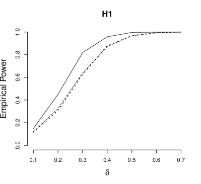
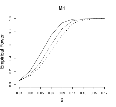
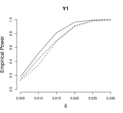
Figure 1: Empirical power of the competing GGF, MHR, and HR methods for testing linear effect for the moderately sparse sampling design. Solid lines indicate results for the MHR method, dashed lines indicate results for the GGF method, and dotted lines indicate results for the HR method. The significance level is $\alpha=0.05$. The number of Monte Carlo experiments is 1,000, and the sample size is $n=500$.

Table 1 summarizes the rejection rates for testing linearity under moderately sparse design. For a large sample size ($n=500$), GGF and MHR maintain the correct nominal levels. The HR method still tends to overestimate the nominal ones, but provides close results to the desired levels. Figure 1 displays the simulated power curves for testing the null hypothesis of the linear covariate effect under the moderate sampling design with the large sample size. The power performance of the methods is a little affected by the change of the sampling design. The methods exhibit minor power loss compared to the results obtained for densely sampled design. The MHR method shows a general advantage over the GGF and HR methods as $\delta$ increases. It performs slightly better than the GGF method under the G1 and G2 settings. For the other settings, the difference between the two methods is more significant. The HR and GGF methods appear to perform very similarly under the H1 and Y1 settings. However, the power of HR is consistently lower than that of GGF for the other data generation settings. For a small sample size ($n=50$), the GGF method tends to underestimate lower nominal levels (1% and 5%), while the MHR method produces significantly higher empirical rejection rates than the nominal levels of 5% and 10%. As in the dense case, there is an especially pronounced difference between the empirical levels for the HR method and the nominal levels. Both GGF and MHR result in more stable Type I errors for $n=100$. We notice that the empirical levels decrease significantly as the sample size increases, but the HR method still produces inflated Type I error rates. Similar to the dense case with the moderate sample size, MHR performs better than GGF in terms of power under all settings. The power of the methods increases at a slower rate as the sample size decreases.

Table 1 about here.

Tables S2 in the Supplementary Material (Appendix A.3) reports the probability of rejecting the null hypothesis of linear relationship for sparse sampling design. The Type I error rates are similar to those of the moderately sparse design except for the M1 data generation setting. For the M1 setting, we notice that all three methods have very inflated rejection probabilities. Moreover, the rejection rates for the GGF and MHR methods are not decreasing as the sample size increases. The problem here might be that there are very few observations per curve, so the estimation performance of the FPCA is affected by the sparsity level of the data. Hence, the methods fail to estimate the Type I error rates accurately. The Supplementary Material includes additional simulation results (Table S3), which indicate that adding few more observations per curve—that is, making the data less sparse, improves the performance of GGF and MHR considerably. As for power comparison, the ordering of the methods does not change except that the HR method produces sightly better results than GGF under the Y1 setting for the large sample size. In general, all three methods lose power as the functional data becomes more sparse, as expected.

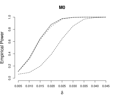
Figure 2: Empirical power of the competing GGF, MHR, and KSM methods for testing no effect for the moderately sparse sampling design. Solid lines indicate results for the MHR method, dashed lines indicate results for the GGF method, and dotted lines indicate results for the KSM method. The significance level is $\alpha=0.05$. The number of Monte Carlo experiments is 1,000, and the sample size is $n=500$.

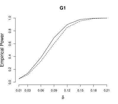
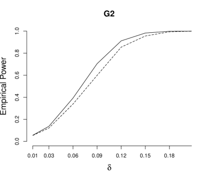
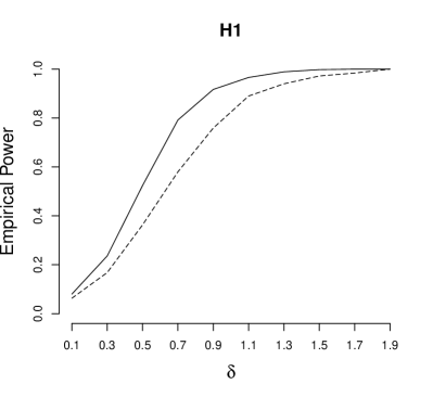
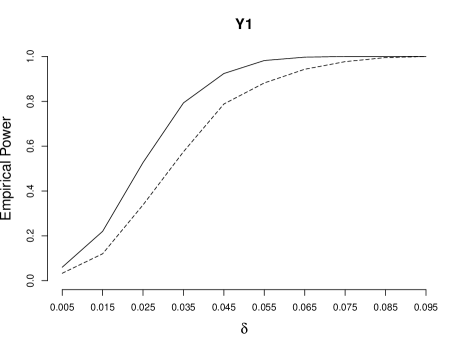
Figure S6: Empirical power of the competing GGF and MHR methods for testing linear effect for the moderately sparse sampling design. Solid lines indicate results for the MHR method and dashed lines indicate results for the GGF method. The significance level is $\alpha=0.05$. The number of Monte Carlo experiments is 1,000, and the sample size is $n=100$.

For testing nullity, Table 2 shows the Type I error rates of the GGF, MHR, and KSM methods. Our results indicate that the rejection probabilities do not appear to change much as the grid of points for the functional covariate becomes more sparse. The rejection rates are mostly within two standard errors of the correct levels for all the designs and various sample sizes, which means that all three methods result in reasonable Type I errors. For all sampling designs, GGF provides more conservative results for the G0 setting than those for the M0 setting. Furthermore, when $n=500$, GGF provides more conservative results than those for MHR and KSM under the G0 data generation setting. The methods still provide good rejection probabilities as the sample size decreases. Only MHR seems to provide relatively conservative results for $n=50$ under the G0 data generation setting. The methods have comparable power for all sample sizes. According to Figure S6 (Appendix B.1), for dense sampling design with a large sample size, the power functions for MHR and KSM are very close to each other such that they overlap. The GGF method is falling dramatically behind these two methods in terms of the power performance. When $n=100$, the KSM outperforms MHR under the G0 setting. Figures 2 and S7 (Appendix B.2)show the power performance of the methods for moderately sampled data with large and moderate sample sizes, respectively. Similar to the previous results, the MHR and KSM methods have good power properties and that they outperform the GGF method substantially both under the G0 and M0 data generation settings when $n=500$. For a moderate sample size ($n=100$), in particular, KSM is more powerful than MHR under the G0 setting. We notice that the power curves for sparse design are very similar to those obtained for moderately sparse design.

Table 2 about here.

We also compare the computational costs of the four methods for 10 simulation runs of the M0 and M1 data generation settings under dense design with the sample size $n=100$. The simulations were run on a 2.3 GHz DELL Quad Processor AMD Opteron with 512 Gb of RAM. The KSM method simulated the data in approximately 3 seconds and the MHR method did so in 4 seconds, which indicates that MHR runs almost as fast as KSM. The GGF method took roughly 12 seconds. The HR method was by far the slowest method, with a computation time of 159 seconds.

To sum up, the HR method falls well behind the MHR and GGF methods, because it provides inaccurate size and power results and has computational complexity. Despite the fact that the GGF method produces results rather close to those for the MHR method for some cases, it still has the disadvantage of being computationally more expensive. Our extensive simulation studies indicate that, for testing linearity, the MHR method outperforms its competitors with regard to approximately close empirical levels, high power rates, and computational efficiency. For testing nullity, both MHR and KSM perform similarly in terms size and power performance for the large sample size. For a moderate sample size, there is no uniform best method; however, based on the results we recommend the KSM method.

Table 1: Testing linearity: Comparison of the estimated Type I error rates of the GGF, MHR, and HR methods in the context of moderately sparse functional data. The data generation settings are G1, G2, H1, M1, and Y1. The number of Monte Carlo experiments is 5,000, and the sample sizes are 50, 100, and 500. Standard errors are shown in parentheses.

		GGF			MHR			HR
	$\boldsymbol{\alpha}$	n=50	n=100	n=500	n=50	n=100	n=500	n=50	n=100	n=500
	0.01	0.005(0.001)	0.008(0.001)	0.010(0.001)	0.011(0.001)	0.011(0.001)	0.009(0.001)	0.087(0.004)	0.036(0.003)	0.012(0.002)
G1	0.05	0.049(0.003)	0.050(0.003)	0.051(0.003)	0.058(0.003)	0.048(0.003)	0.048(0.003)	0.199(0.006)	0.105(0.004)	0.060(0.003)
	0.10	0.118(0.005)	0.108(0.004)	0.100(0.004)	0.115(0.005)	0.100(0.004)	0.098(0.004)	0.288(0.006)	0.179(0.005)	0.123(0.005)
	0.01	0.004(0.001)	0.008(0.001)	0.011(0.001)	0.013(0.002)	0.012(0.002)	0.011(0.001)	0.093(0.004)	0.035(0.003)	0.013(0.002)
G2	0.05	0.049(0.003)	0.048(0.003)	0.049(0.003)	0.054(0.003)	0.047(0.003)	0.051(0.003)	0.209(0.006)	0.105(0.004)	0.059(0.003)
	0.10	0.119(0.005)	0.108(0.004)	0.103(0.004)	0.109(0.004)	0.103(0.004)	0.104(0.004)	0.299(0.006)	0.173(0.005)	0.119(0.005)
	0.01	0.006(0.001)	0.008(0.001)	0.012(0.002)	0.015(0.002)	0.014(0.002)	0.010(0.001)	0.093(0.004)	0.035(0.003)	0.012(0.002)
H1	0.05	0.046(0.003)	0.052(0.003)	0.056(0.003)	0.063(0.003)	0.053(0.003)	0.051(0.003)	0.206(0.006)	0.115(0.005)	0.060(0.003)
	0.10	0.113(0.004)	0.109(0.004)	0.099(0.004)	0.113(0.004)	0.105(0.004)	0.100(0.004)	0.295(0.006)	0.184(0.005)	0.112(0.004)
	0.01	0.002(0.001)	0.005(0.001)	0.011(0.001)	0.014(0.002)	0.012(0.002)	0.011(0.001)	0.095(0.004)	0.039(0.003)	0.015(0.002)
M1	0.05	0.036(0.003)	0.039(0.003)	0.050(0.003)	0.064(0.003)	0.052(0.003)	0.051(0.003)	0.210(0.006)	0.115(0.005)	0.059(0.003)
	0.10	0.102(0.004)	0.094(0.004)	0.097(0.004)	0.121(0.005)	0.107(0.004)	0.103(0.004)	0.300(0.006)	0.187(0.005)	0.115(0.005)
	0.01	0.005(0.001)	0.014(0.002)	0.013(0.002)	0.016(0.002)	0.011(0.001)	0.010(0.001)	0.098(0.004)	0.038(0.003)	0.016(0.002)
Y1	0.05	0.058(0.003)	0.055(0.003)	0.067(0.004)	0.062(0.003)	0.049(0.003)	0.050(0.003)	0.222(0.006)	0.118(0.005)	0.061(0.003)
	0.10	0.125(0.005)	0.116(0.005)	0.119(0.004)	0.126(0.005)	0.100(0.004)	0.100(0.004)	0.320(0.007)	0.193(0.006)	0.116(0.005)

Table 2: Testing nullity: Comparison of the estimated Type I error rates of the GGF, MHR, and KSM methods in the context of dense, moderately sparse, and sparse functional data. The data generation settings are G0 and M0. The number of Monte Carlo experiments is 5,000, and the sample sizes are 50, 100, and 500. Standard errors are shown in parentheses.

		GGF			MHR			KSM
	$\boldsymbol{\alpha}$	n=50	n=100	n=500	n=50	n=100	n=500	n=50	n=100	n=500
Dense
	0.01	0.008(0.001)	0.010(0.001)	0.010(0.001)	0.008(0.001)	0.009(0.001)	0.010(0.001)	0.009(0.001)	0.013(0.002)	0.008(0.001)
G0	0.05	0.048(0.003)	0.049(0.003)	0.046(0.003)	0.043(0.003)	0.049(0.003)	0.050(0.003)	0.051(0.003)	0.055(0.003)	0.049(0.003)
	0.10	0.101(0.004)	0.097(0.004)	0.095(0.004)	0.084(0.004)	0.097(0.004)	0.108(0.004)	0.100(0.004)	0.105(0.004)	0.098(0.004)
	0.01	0.008(0.001)	0.010(0.001)	0.012(0.002)	0.011(0.001)	0.010(0.001)	0.010(0.001)	0.010(0.001)	0.009(0.001)	0.009(0.001)
M0	0.05	0.047(0.003)	0.052(0.003)	0.052(0.003)	0.050(0.003)	0.048(0.003)	0.055(0.003)	0.049(0.003)	0.048(0.003)	0.054(0.003)
	0.10	0.103(0.004)	0.103(0.004)	0.104(0.004)	0.099(0.004)	0.097(0.004)	0.106(0.004)	0.101(0.004)	0.099(0.004)	0.107(0.004)
Moderate
	0.01	0.009(0.001)	0.010(0.001)	0.010(0.001)	0.008(0.001)	0.009(0.001)	0.011(0.001)	0.010(0.001)	0.011(0.001)	0.008(0.001)
G0	0.05	0.048(0.003)	0.048(0.003)	0.046(0.003)	0.043(0.003)	0.050(0.003)	0.052(0.003)	0.050(0.003)	0.055(0.003)	0.051(0.003)
	0.10	0.102(0.004)	0.096(0.004)	0.095(0.004)	0.086(0.004)	0.098(0.004)	0.104(0.004)	0.103(0.004)	0.104(0.004)	0.098(0.004)
	0.01	0.009(0.001)	0.010(0.001)	0.011(0.001)	0.010(0.001)	0.009(0.001)	0.009(0.001)	0.012(0.002)	0.008(0.001)	0.008(0.001)
M0	0.05	0.050(0.003)	0.051(0.003)	0.052(0.003)	0.049(0.003)	0.049(0.003)	0.054(0.003)	0.048(0.003)	0.046(0.003)	0.055(0.003)
	0.10	0.104(0.004)	0.104(0.004)	0.104(0.004)	0.098(0.104)	0.098(0.004)	0.108(0.004)	0.099(0.004)	0.093(0.004)	0.108(0.004)
Sparse
	0.01	0.009(0.001)	0.009(0.001)	0.010(0.001)	0.008(0.001)	0.009(0.001)	0.011(0.001)	0.010(0.001)	0.012(0.002)	0.011(0.001)
G0	0.05	0.048(0.003)	0.047(0.003)	0.046(0.003)	0.044(0.003)	0.050(0.003)	0.050(0.003)	0.057(0.003)	0.046(0.003)	0.046(0.003)
	0.10	0.101(0.004)	0.095(0.004)	0.094(0.004)	0.092(0.004)	0.097(0.004)	0.106(0.004)	0.102(0.004)	0.099(0.004)	0.099(0.004)
	0.01	0.009(0.001)	0.011(0.001)	0.011(0.001)	0.011(0.001)	0.010(0.001)	0.011(0.001)	0.012(0.002)	0.009(0.001)	0.010(0.001)
M0	0.05	0.049(0.003)	0.050(0.003)	0.053(0.003)	0.050(0.003)	0.049(0.003)	0.054(0.003)	0.049(0.003)	0.048(0.003)	0.052(0.003)
	0.10	0.104(0.004)	0.103(0.004)	0.105(0.004)	0.102(0.004)	0.096(0.004)	0.108(0.004)	0.100(0.004)	0.101(0.004)	0.105(0.004)

6 Data Analysis

We consider the application of these methods to a food quality control problem. The Tecator data set has been commonly used to predict the fat content of meat samples and is found at http://lib.stat.cmu.edu/datasets/tecator.

This data set includes measurements of a 100-channel spectrum of absorbances, in addition to fat, protein, and moisture (water) content from $n=215$ finely chopped pure meat samples. For each sample of meat, a 100-channel near-infrared (NIR) spectrum of absorbances is calculated as a log transform of the transmittance obtained by the analyzer and recorded. The absorbances for a meat sample can be deemed to be discrete realizations of random smooth curves, $X_{i}(\cdot)$. The absorbance trajectories versus wavelength are displayed in Figure 3.

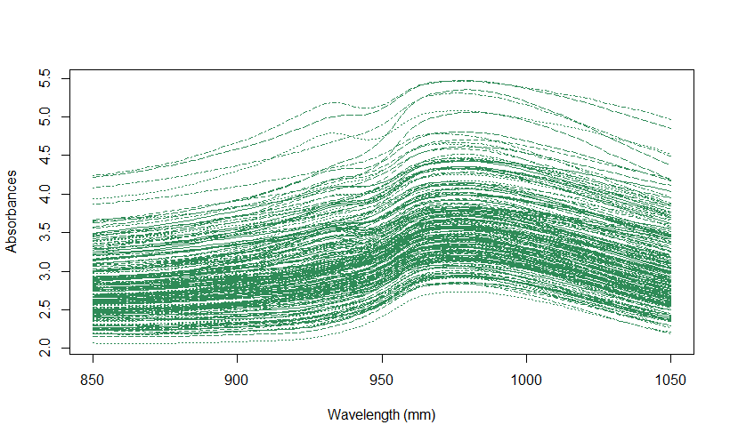
Figure 3: Absorbance trajectories concerning 215 samples of finely chopped pure meat.

The data were first analyzed by Borggaard and Thodberg [1992], who trained neural network models to predict the fat content. Yao and Müller [2010] proposed a functional quadratic regression model to predict the fat content depending on the absorbance trajectories. For the same purpose, Febrero-Bande and González-Manteiga [2013] developed an algorithm for functional regression models whose response variable comes from an exponential family. Rather than focusing on prediction, Horváth and Reeder [2013] and García-Portugués et al. [2014] used this data set to investigate whether a linear dependence existed between the functional covariate and the scalar response.

The goal of this section is to test whether the association between the spectra of absorbances (functional predictor) and each of the measures of fat, protein, or water content of the meat samples (scalar responses) is null or not. In this regard, we employ the three methods—GGF, MHR and KSM—and we discuss whether there is evidence against a null association. In addition, we investigate whether the existing association is linear by employing the three methods—GGF, MHR and HR. A significance level of $\alpha=0.05$ is used. Because we use the same data set with three different methods for each response (fat, protein, and moisture), we apply a Bonferroni correction to account for multiple testing. The adjusted significance level is $\alpha=0.05/3=0.0167$.

Table 3 about here.

The results for the nullity test are shown in Table 3. These results are not very surprising, because previous analyses [Horváth and Reeder, 2013, García-Portugués et al., 2014] have determined that an association exists between each of the responses and the functional covariate. Our analysis confirms this, because all $p$-values are less than $\alpha=0.0167$. More interesting results are obtained by the linear tests (Table 3), because we can draw different conclusions depending on the test we use. The $p$-values of the GGF method are greater than $\alpha$ for both fat and water content, which means that this test produces no evidence to reject the null hypothesis of a linear relationship between percentage of fat and the absorbance trajectories, or between the moisture and the same functional covariate. A different conclusion can be drawn if we use the MHR or the HR method, because their $p$-values are less than $\alpha$ for all responses. These results are expected as in our simulation study; the GGF method showed consistently less power than the MHR test for various data structures.

Table 3: $p$-values for each of the methods for testing null effect and linear effect of the spectra of absorbances on response variables fat, protein, and water content. The significance level is $\alpha=0.0167$.

	Nullity				Linearity
	Fat	Water	Protein		Fat	Water	Protein
GGF	0.000*	0.000*	0.000*	GGF	0.029	0.017	0.009*
MHR	0.000*	0.000*	0.000*	MHR	0.000*	0.000*	0.000*
KSM	0.000*	0.000*	0.000*	HR	0.000*	0.000*	0.000*

• Note. *Significant at the $p<0.0167$ level.

References

The Supplement Material contains two sections. Section A presents additional simulation results (empirical rejection rates and power curves) for testing linearity in the context of dense, moderately sparse, and sparse functional data. Section B includes additional power curves for testing nullity in the context of dense, moderately sparse, and sparse functional data.

G Simulation results for testing linearity

G.1 Type I error rates and power curves for dense sampling design

Table S4: Testing linearity: Comparison of the estimated Type I error rates of the GGF, MHR, and HR methods in the context of dense functional data. The data generation settings are G1, G2, H1, M1, and Y1. The number of Monte Carlo experiments is 5,000, and the sample sizes are 50, 100, and 500. Standard errors are shown in parentheses.

		GGF			MHR			HR
	$\boldsymbol{\alpha}$	n=50	n=100	n=500	n=50	n=100	n=500	n=50	n=100	n=500
	0.01	0.011(0.001)	0.009(0.001)	0.009(0.001)	0.011(0.001)	0.012(0.002)	0.009(0.001)	0.090(0.004)	0.033(0.003)	0.011(0.001)
G1	0.05	0.073(0.004)	0.054(0.003)	0.052(0.003)	0.061(0.003)	0.052(0.003)	0.048(0.003)	0.200(0.006)	0.104(0.004)	0.060(0.003)
	0.10	0.157(0.005)	0.112(0.004)	0.099(0.004)	0.116(0.005)	0.098(0.004)	0.099(0.004)	0.288(0.006)	0.176(0.005)	0.121(0.005)
	0.01	0.010(0.001)	0.009(0.001)	0.011(0.001)	0.012(0.002)	0.011(0.001)	0.012(0.002)	0.091(0.004)	0.033(0.003)	0.012(0.002)
G2	0.05	0.066(0.004)	0.056(0.003)	0.051(0.003)	0.054(0.003)	0.048(0.003)	0.053(0.003)	0.203(0.006)	0.105(0.004)	0.060(0.003)
	0.10	0.151(0.005)	0.115(0.005)	0.104(0.004)	0.110(0.004)	0.101(0.004)	0.106(0.004)	0.294(0.006)	0.170(0.005)	0.122(0.005)
	0.01	0.013(0.002)	0.009(0.001)	0.012(0.002)	0.016(0.002)	0.014(0.002)	0.010(0.001)	0.097(0.004)	0.036(0.003)	0.012(0.002)
H1	0.05	0.076(0.004)	0.055(0.003)	0.055(0.003)	0.062(0.003)	0.052(0.003)	0.052(0.003)	0.208(0.006)	0.111(0.004)	0.059(0.003)
	0.10	0.154(0.005)	0.120(0.005)	0.105(0.004)	0.114(0.004)	0.107(0.004)	0.102(0.004)	0.297(0.006)	0.185(0.005)	0.112(0.004)
	0.01	0.002(0.001)	0.005(0.001)	0.011(0.001)	0.015(0.002)	0.011(0.001)	0.011(0.001)	0.087(0.004)	0.038(0.003)	0.017(0.002)
M1	0.05	0.034(0.003)	0.038(0.003)	0.049(0.003)	0.065(0.003)	0.052(0.003)	0.051(0.003)	0.202(0.006)	0.114(0.004)	0.058(0.003)
	0.10	0.099(0.004)	0.092(0.004)	0.097(0.004)	0.122(0.005)	0.107(0.004)	0.103(0.004)	0.291(0.006)	0.180(0.005)	0.112(0.004)
	0.01	0.012(0.002)	0.008(0.001)	0.008(0.001)	0.013(0.002)	0.008(0.001)	0.010(0.001)	0.084(0.004)	0.038(0.003)	0.013(0.002)
Y1	0.05	0.074(0.004)	0.053(0.003)	0.055(0.003)	0.057(0.003)	0.046(0.003)	0.046(0.003)	0.199(0.006)	0.116(0.005)	0.059(0.003)
	0.10	0.160(0.005)	0.124(0.005)	0.103(0.004)	0.107(0.004)	0.097(0.004)	0.093(0.004)	0.290(0.006)	0.183(0.005)	0.111(0.004)

Table S1 about here.

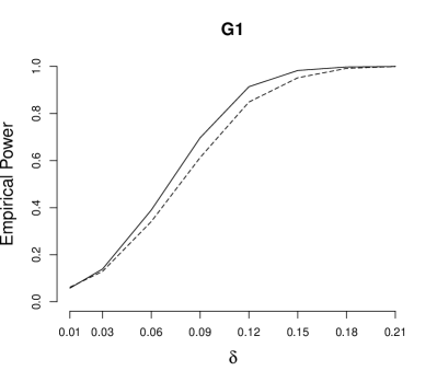
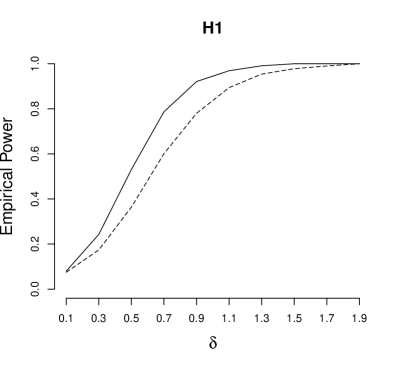
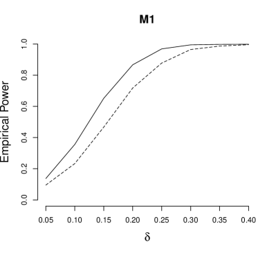
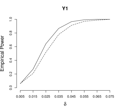
Figure S4: Empirical power of the competing GGF and MHR methods for testing linear effect for the dense sampling design. Solid lines indicate results for the MHR method and dashed lines indicate results for the GGF method. The significance level is $\alpha=0.05$. The number of Monte Carlo experiments is 1,000, and the sample size is $n=100$.

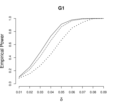
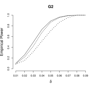
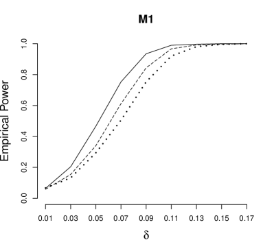
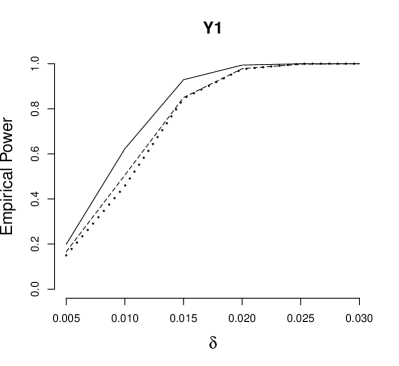
Figure S5: Empirical power of the competing GGF, MHR, and HR methods for testing linear effect for the dense sampling design. Solid lines indicate results for the MHR method, dashed lines indicate results for the GGF method, and dotted lines indicate results for the HR method. The significance level is $\alpha=0.05$. The number of Monte Carlo experiments is 1,000, and the sample size is $n=500$.

G.2 Power curves for moderate sampling design

G.3 Type I error rates and power curves for sparse sampling design

Table S5: Testing linearity: Comparison of the estimated Type I error rates of the GGF, MHR, and HR methods in the context of sparse functional data. The data generation settings are G1, G2, H1, M1, and Y1. The number of Monte Carlo experiments is 5,000, and the sample sizes are 50, 100, and 500. Standard errors are shown in parentheses.

		GGF			MHR			HR
	$\boldsymbol{\alpha}$	n=50	n=100	n=500	n=50	n=100	n=500	n=50	n=100	n=500
	0.01	0.006(0.001)	0.008(0.001)	0.009(0.001)	0.015(0.002)	0.013(0.002)	0.011(0.001)	0.105(0.004)	0.039(0.003)	0.012(0.002)
G1	0.05	0.045(0.003)	0.047(0.003)	0.051(0.003)	0.059(0.003)	0.049(0.003)	0.056(0.003)	0.224(0.006)	0.120(0.005)	0.060(0.003)
	0.10	0.110(0.004)	0.106(0.004)	0.102(0.004)	0.116(0.005)	0.097(0.004)	0.104(0.004)	0.315(0.007)	0.191(0.006)	0.117(0.005)
	0.01	0.004(0.001)	0.007(0.001)	0.009(0.001)	0.013(0.002)	0.012(0.002)	0.013(0.002)	0.097(0.004)	0.036(0.003)	0.013(0.002)
G2	0.05	0.038(0.003)	0.053(0.003)	0.049(0.003)	0.056(0.003)	0.054(0.003)	0.053(0.003)	0.213(0.006)	0.117(0.005)	0.063(0.003)
	0.10	0.101(0.004)	0.108(0.004)	0.103(0.004)	0.117(0.005)	0.104(0.004)	0.105(0.004)	0.310(0.007)	0.190(0.006)	0.119(0.005)
	0.01	0.006(0.001)	0.008(0.001)	0.012(0.002)	0.015(0.002)	0.013(0.002)	0.012(0.002)	0.094(0.004)	0.036(0.003)	0.013(0.002)
H1	0.05	0.050(0.003)	0.049(0.003)	0.052(0.003)	0.061(0.003)	0.055(0.003)	0.051(0.003)	0.218(0.006)	0.113(0.004)	0.057(0.003)
	0.10	0.117(0.005)	0.105(0.004)	0.100(0.004)	0.119(0.005)	0.108(0.004)	0.100(0.004)	0.312(0.007)	0.182(0.005)	0.115(0.005)
	0.01	0.035(0.003)	0.069(0.004)	0.155(0.005)	0.108(0.004)	0.169(0.005)	0.293(0.006)	0.170(0.005)	0.110(0.004)	0.085(0.004)
M1	0.05	0.101(0.004)	0.135(0.005)	0.218(0.006)	0.181(0.005)	0.230(0.006)	0.335(0.007)	0.297(0.006)	0.203(0.006)	0.150(0.005)
	0.10	0.189(0.006)	0.208(0.006)	0.278(0.006)	0.239(0.006)	0.285(0.006)	0.378(0.007)	0.389(0.007)	0.280(0.006)	0.214(0.006)
	0.01	0.006(0.002)	0.008(0.002)	0.008(0.002)	0.013(0.002)	0.014(0.002)	0.008(0.001)	0.105(0.004)	0.038(0.003)	0.010(0.001)
Y1	0.05	0.045(0.004)	0.052(0.004)	0.042(0.004)	0.064(0.003)	0.054(0.003)	0.047(0.003)	0.237(0.006)	0.118(0.005)	0.058(0.003)
	0.10	0.114(0.006)	0.102(0.006)	0.087(0.006)	0.121(0.005)	0.103(0.004)	0.097(0.004)	0.337(0.007)	0.195(0.006)	0.104(0.004)

Table S6: Testing linearity: Comparison of the estimated Type I error rates of the GGF and MHR methods in the context of sparse functional data under the M1 setting. The observation points are sampled per curve without replacement from the discrete uniform distribution $\mbox{Unif}\{9,\ldots,12\}$. The number of Monte Carlo experiments is 5,000, and the sample sizes are 50, 100, and 500. Standard errors are shown in parentheses.

	GGF			MHR
$\boldsymbol{\alpha}$	n=50	n=100	n=500	n=50	n=100	n=500
0.01	0.003(0.001)	0.006(0.001)	0.011(0.001)	0.019(0.001)	0.018(0.002)	0.018(0.001)
0.05	0.037(0.003)	0.043(0.003)	0.051(0.003)	0.072(0.003)	0.065(0.003)	0.059(0.003)
0.10	0.106(0.004)	0.098(0.004)	0.099(0.004)	0.138(0.005)	0.116(0.004)	0.111(0.004)

Table S2 about here.

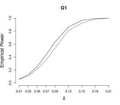
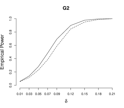
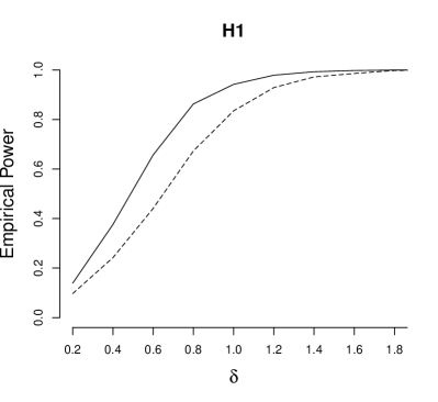
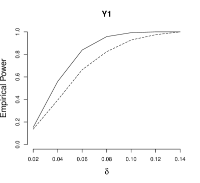
Figure S7: Empirical power of the competing GGF and MHR methods for testing linear effect for the sparse sampling design. Solid lines indicate results for the MHR method and dashed lines indicate results for the GGF method. The significance level is $\alpha=0.05$. The number of Monte Carlo experiments is 1,000, and the sample size is $n=100$.

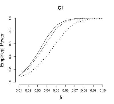
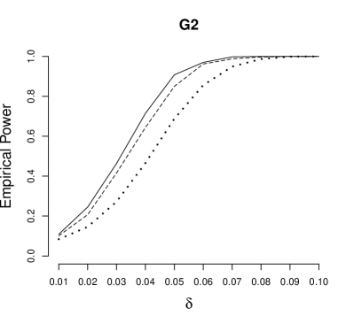
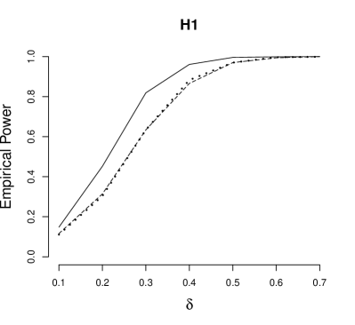
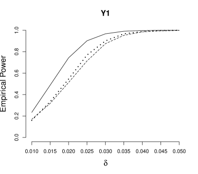
Figure S8: Empirical power of the competing GGF, MHR, and HR methods for testing linear effect for the sparse sampling design. Solid lines indicate results for the MHR method, dashed lines indicate results for the GGF method, and dotted lines indicate results for the HR method. The significance level is $\alpha=0.05$. The number of Monte Carlo experiments is 1,000, and the sample size is $n=500$.

H Simulation results for testing nullity

H.1 Power curves for dense sampling design

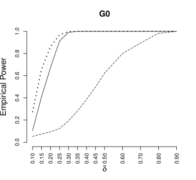
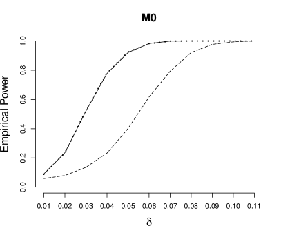
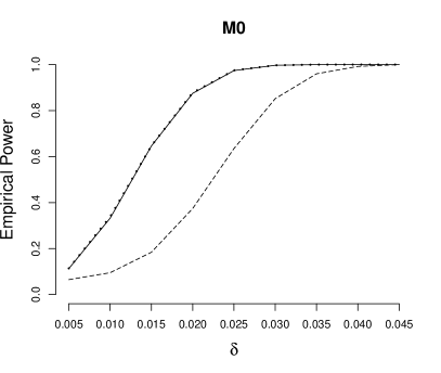
Figure S9: Empirical power of the competing GGF, MHR, and KSM methods for testing no effect for the dense sampling design with sample sizes $n=100$ (1st row) and $n=500$ (2nd row), respectively. Solid lines indicate results for the MHR method, dashed lines indicate results for the GGF method, and dotted lines indicate results for the KSM method. The significance level is $\alpha=0.05$. The number of Monte Carlo experiments is 1,000.

H.2 Power curves for moderate sampling design

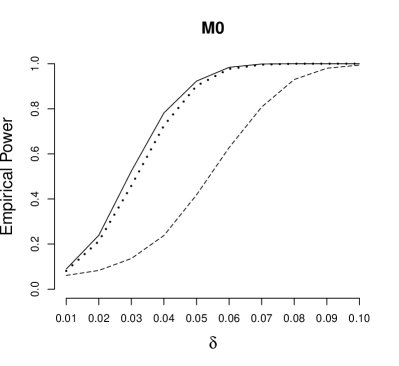
Figure S10: Empirical power of the competing GGF, MHR, and KSM methods for testing no effect for the moderate sampling design. Solid lines indicate results for the MHR method, dashed lines indicate results for the GGF method, and dotted lines indicate results for the KSM method. The significance level is $\alpha=0.05$. The number of Monte Carlo experiments is 1,000, and the sample size is $n=100$.

H.3 Power curves for sparse sampling design

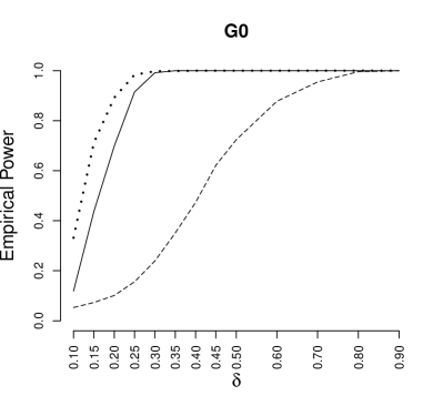
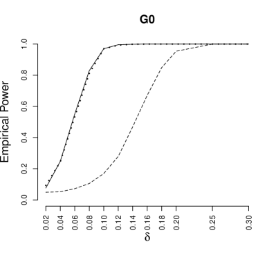
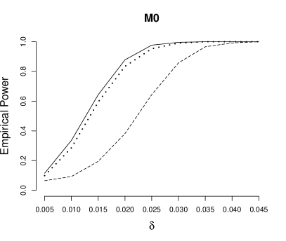
Figure S11: Empirical power of the competing GGF, MHR, and KSM methods for testing no effect for the sparse sampling design with sample sizes $n=100$ (1st row) and $n=500$ (2nd row), respectively. Solid lines indicate results for the MHR method, dashed lines indicate results for the GGF method, and dotted lines indicate results for the KSM method. The significance level is $\alpha=0.05$. The number of Monte Carlo experiments is 1,000.

References

- Borggaard and Thodberg [1992] Borggaard C, Thodberg HH. Optimal minimal neural interpretation of spectra. Analytical chemistry 1992;64(5):545–51.
- Cai et al. [2006] Cai TT, Hall P, et al. Prediction in functional linear regression. The Annals of Statistics 2006;34(5):2159–79.
- Cardot et al. [2003] Cardot H, Ferraty F, Mas A, Sarda P. Testing hypotheses in the functional linear model. Scandinavian Journal of Statistics 2003;30(1):241–55.
- Cardot et al. [1999] Cardot H, Ferraty F, Sarda P. Functional linear model. Statistics & Probability Letters 1999;45(1):11–22.
- Cardot et al. [2004] Cardot H, Goia A, Sarda P. Testing for no effect in functional linear regression models, some computational approaches. Communications in Statistics-Simulation and Computation 2004;33(1):179–99.
- Crainiceanu and Ruppert [2004] Crainiceanu CM, Ruppert D. Likelihood ratio tests in linear mixed models with one variance component. Journal of the Royal Statistical Society: Series B (Statistical Methodology) 2004;66(1):165–85. URL: http://doi.wiley.com/10.1111/j.1467-9868.2004.00438.x. doi:10.1111/j.1467-9868.2004.00438.x.
- Crambes et al. [2009] Crambes C, Kneip A, Sarda P. Smoothing splines estimators for functional linear regression. The Annals of Statistics 2009;:35–72.
- Delsol et al. [2011] Delsol L, Ferraty F, Vieu P. Structural test in regression on functional variables. Journal of Multivariate Analysis 2011;102(3):422–47. URL: http://linkinghub.elsevier.com/retrieve/pii/S0047259X10002095. doi:10.1016/j.jmva.2010.10.003.
- Febrero-Bande and González-Manteiga [2013] Febrero-Bande M, González-Manteiga W. Generalized additive models for functional data. Test 2013;22(2):278–92.
- Ferraty and Vieu [2006] Ferraty F, Vieu P. Nonparametric functional data analysis: theory and practice. Springer Science & Business Media, 2006.