Galactocentric variation of the gas-to-dust ratio and its relation with metallicity

Abstract

Context. The assumption of a gas-to-dust mass ratio $\gamma$ is a common approach to estimate the basic properties of molecular clouds, such as total mass and column density of molecular hydrogen, from (sub)mm continuum observations of the dust. In the Milky Way a single value is used at all galactocentric radii, independently of the observed metallicity gradients. Both models and extragalactic observations suggest that this quantity increases for decreasing metallicity $Z$, typical of the outer regions in disks, where fewer heavy elements are available to form dust grains.

Aims. We aim to investigate the variation of the gas-to-dust ratio as a function of galactocentric radius and metallicity, to allow a more accurate characterisation of the quantity of molecular gas across the galactic disk, as derived from observations of the dust.

Methods. Observations of the optically thin C¹⁸O (2–1) transition were obtained with the APEX telescope for a sample of 23 massive and dense star-forming regions in the far outer Galaxy (galactocentric distance greater than $14\usk\mathrm{kpc}$). From the modelling of this line and of the spectral energy distribution of the selected clumps we computed the gas-to-dust ratio and compared it to that of well-studied sources from the ATLASGAL TOP100 sample in the inner galactic disk.

Results. The gradient in $\gamma$ is found to be $0.087^{{+0.047}}_{{-0.025}}\usk\mathrm{dex}\usk\mathrm{kpc}^{-1}$ (or equivalently $\gamma\propto Z^{-1.4^{{+0.3}}_{{-1.0}}}$). The dust-to-metal ratio, decreases with galactocentric radius, which is the most common situation also for external late-type galaxies. This suggests that grain growth dominates over destruction. The predicted $\gamma$ is in excellent agreement with the estimates in Magellanic clouds, for the appropriate value of $Z$.

1 Introduction

In the past decade many surveys of the galactic plane have been carried out in the continuum, covering wavelengths from the millimetre regime to the infrared (IR). They provide a complete picture of the dust emission, tracing both very cold material (at millimetre, sub-mm and far-IR wavelengths; for example ATLASGAL, Schuller et al. 2009, and Hi-GAL, Molinari et al. 2010), and hot dust and PAHs (in the mid- and near-IR; for example MSX, Egan et al. 2003, MIPSGAL, Carey et al. 2009, WISE, Wright et al. 2010). The temperature, mass and column density of the dust can be estimated by constructing and modelling the spectral energy distribution of the thermal dust emission (SED; e.g. König et al., 2017). The dust, however, constitutes only a minor fraction of the total mass of molecular clouds. One has to assume a gas-to-dust mass ratio ($\gamma$) to derive the mass and column density of molecular hydrogen. A direct, local determination shows that the hydrogen-to-dust mass ratio is $\sim 100$, corresponding to a gas-to-dust mass ratio $\gamma\approx 136$, when accounting for helium (Draine et al., 2007). Current research uses a constant value of the gas-to-dust ratio irrespective of the galactocentric distance of the cloud (typically $100-150$, e.g. Elia et al., 2013, 2017; König et al., 2017), and while these values are reasonable within the solar circle they are not likely to be reliable for the outer parts of the disk, where the metallicity and average disk surface density might be substantially lower.

Heavy elements are the main constituents of dust grains, and therefore when their abundance with respect to hydrogen changes, dust may be influenced too. Models combining chemical evolution of the Galaxy with dust evolution indeed suggest that $\gamma$ increases with decreasing metallicity $Z$ (Dwek, 1998; Mattsson & Andersen, 2012; Hirashita & Harada, 2017). This is also supported by observations in nearby galaxies (e.g. Sandstrom et al., 2013).

Except for a few cases, the data for external galaxies are averaged over the entire galaxy, and in all cases optically thick CO lines are used to obtain the mass of molecular gas. Moreover, in studies in which the gradient in $\gamma$ with $Z$ can be spatially resolved, the resolution is of the order of a kpc, introducing large uncertainties, for example, by assuming a uniform single temperature for dust or a specific calibration in deriving the metallicity (e.g. Sandstrom et al., 2013). As Mattsson & Andersen (2012) discuss, this could lead to a dust content which, in the central regions, often is larger than the amount of available metals in the interstellar medium (ISM).

The study of the metallicity-$\gamma$ relation in the Milky Way not only opens the possibility to have, for the first time, more accurate estimates of the amount of molecular gas in clouds, but also provides the possibility to explore it on spatial scales and sensitivities that are extremely challenging to obtain, if not inaccessible, in galaxies other than our own. Issa et al. (1990) studied how the gradient in gas-to-dust ratio depends on the galactocentric radius, but for a limited range of $R_{\mathrm{GC}}$ ($9-11\usk\mathrm{kpc}$) and using optically thick CO lines to estimate the amount of molecular gas, via the integrated intensity of the CO (1–0) line-to-molecular mass conversion factor $X_{\mathrm{CO}}$.

In this work we use a sample of 23 sources in the far outer Galaxy, complemented by 57 sources from the ATLASGAL TOP100 in the inner Galaxy (Fig. 1) to expand this pioneering work, exploring the variation of $\gamma$ across the entire disk of the Milky Way. This opens up the possibility of using the appropriate value of the gas-to-dust ratio to obtain more precise estimates of the very basic properties of molecular clouds throughout the Milky Way from publicly available surveys, such as the total mass and H₂ column density. From these quantities it is possible to derive molecular abundances and, in combination with complete surveys of the galactic disk, a reliable distribution of mass of molecular gas in the Milky Way.

2 Observations and sample selection

From the Wouterloot & Brand (1989) IRAS/CO catalogue and that compiled by König et al. (in prep.) using ¹²CO(2–1) and ¹³CO (2–1), we selected a sample of 23 sources in the far outer Galaxy ($R_{\mathrm{GC}}>14\usk\mathrm{kpc}$; FOG) with the following criteria: i) the source must be associated with IR emission in WISE images ii) Herschel data must be available to estimate the dust content, and iii) the surface density of dust ($\Sigma_{\mathrm{dust}}$) at the emission peak must exceed $3\times 10^{-5}\usk\mathrm{g}\usk\mathrm{c}\mathrm{m}^{-2}$, or $N_{\mathrm{H_{2}}}=8.75\times 10^{20}\usk\mathrm{c}\mathrm{m}^{-2}$ (i.e. $\Sigma_{gas}\sim 19\usk\mathrm{M_{\odot}}\usk\mathrm{pc}^{-2}$), assuming $\gamma=136$. According to the model of Hirashita & Harada (2017), the latter condition is sufficient to ensure that the vast majority of gas is in molecular form for $Z\gtrsim 0.2\usk Z_{\odot}$. In the FOG, in fact, the metallicity ranges from $\sim 0.5\,Z_{\odot}$ at $R_{\mathrm{GC}}\sim 14\usk\mathrm{kpc}$ to $\sim 0.2\,Z_{\odot}$ at $R_{\mathrm{GC}}\sim 21\usk\mathrm{kpc}$ (using the results in Luck & Lambert, 2011, see Eq. 3). Observations of the Magellanic Clouds also provide support for this statement. The metallicities in the Large and Small Magellanic Clouds (LMC, SMC) are $Z=0.5\,Z_{\odot}$ and $Z=0.2\,Z_{\odot}$, respectively (Russell & Dopita, 1992), encompassing the range of the far outer Galaxy. Observations of the atomic and molecular gas in these galaxies by Roman-Duval et al. (2014) demonstrate that the Hi–H₂ transition occurs at $\approx 30\usk\mathrm{M_{\odot}}\usk\mathrm{pc}^{-2}$ in the LMC and $\approx 80\usk\mathrm{M_{\odot}}\usk\mathrm{pc}^{-2}$ in the SMC. Our criterion on the surface density of dust, when using the gas-to-dust ratios estimated by Roman-Duval et al. (2014) in the Magellanic Clouds, exceeded these observed thresholds: $\Sigma_{gas}\approx 70\usk\mathrm{M_{\odot}}\usk\mathrm{pc}^{-2}$ for $Z=0.5\,Z_{\odot}$ and $\sim 230\usk\mathrm{M_{\odot}}\usk\mathrm{pc}^{-2}$ for $Z=0.2\,Z_{\odot}$.

The selection of only IR-bright sources, still associated with substantial molecular material, implies that we are dealing with clumps in a relatively advanced stage of the star formation process, when CO is not significantly affected by depletion (Giannetti et al., 2014). The sources have been followed-up with single-pointing observations centred on the dust emission peak, as identified in Herschel images, carried out using the APEX-1 receiver at APEX tuned to $218.09\usk\mathrm{G}\mathrm{Hz}$, a setup which includes C¹⁸O(2–1). Here, we have used this transition to estimate the total amount of H₂ at the position of the dust emission peak. The angular resolution of APEX at this frequency is $\sim 28\arcsec$. Observations were performed between September 29 and October 15 2015, and between December 3 and 11 2015. The typical rms noise on the $T_{\mathrm{{A}}}^{*}$-scale ranges between $10\usk\mathrm{m}\mathrm{K}$ and $20\usk\mathrm{m}\mathrm{K}$ at a spectral resolution of $0.4\usk\mathrm{k}\mathrm{m}\usk\mathrm{s}^{-1}$. We converted the antenna temperature $T_{\mathrm{{A}}}^{*}$ to main beam brightness temperature, $T_{\mathrm{{MB}}}$, using $\eta_{\mathrm{MB}}=0.75$.

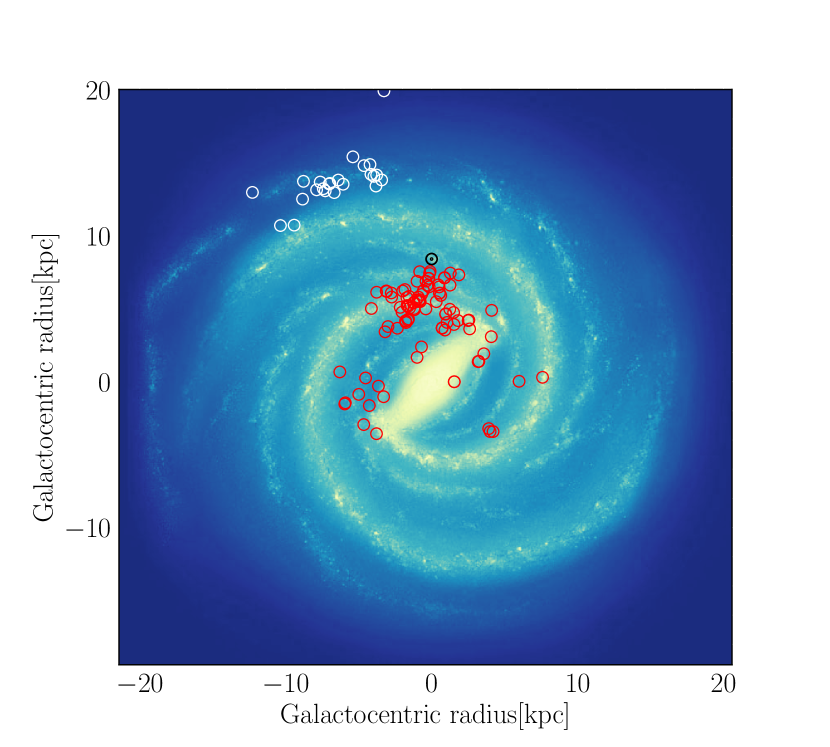
Figure 1: Distribution of the sources considered in this work. In white we show the sources in the FOG, and in red we show clumps from the TOP100 sample. The background image is an artist impression of the Milky Way as seen from the northern galactic pole (courtesy of NASA/JPL-Caltech/R. Hurt – SSC/Caltech). The Sun in at (0, 8.34) kpc.

3 Results

As a first step we constructed the SED for each of the sources in the FOG to obtain the peak mass surface density of the dust. For the SED construction and fitting, we follow the procedure described in König et al. (2017) and adopted in Giannetti et al. (2017) and Urquhart et al. (2017), with minor changes due to the absence of ATLASGAL images for the outer Galaxy. We considered the five Hi-GAL (Molinari et al., 2010) bands (500, 350, 250, 160 and $70\usk\mathrm{\SIUnitSymbolMicro}\mathrm{m}$) from the SPIRE (Griffin et al., 2010) and PACS (Poglitsch et al., 2010) instruments, to reconstruct the cold dust component of the SED. The contribution from a hot embedded component is estimated from mid-IR continuum measurements, using MSX (Egan et al., 2003) and WISE (Wright et al., 2010) images at 21, 14, 12 and $8\usk\mathrm{\SIUnitSymbolMicro}\mathrm{m}$, and 24 and $12\usk\mathrm{\SIUnitSymbolMicro}\mathrm{m}$, respectively.

The flux for each of the bands was calculated using an aperture-and-annulus scheme. The aperture is centred on the emission peak at $250\usk\mathrm{\SIUnitSymbolMicro}\mathrm{m}$ and its size was set to three times the FWHM of a Gaussian fitted to the $250\usk\mathrm{\SIUnitSymbolMicro}\mathrm{m}$ image. The background was calculated as the median flux over an annulus with inner and outer radii of 1.5 and 2.5 the aperture size, respectively. After being normalised to the area of the aperture, the background was subtracted from the flux within the aperture. The uncertainties on the background-corrected fluxes were calculated summing in quadrature the pixel noise of the images and a flux calibration uncertainty. We adopted a calibration uncertainty of $20\%$ for the 350, 250, 160 and $70\usk\mathrm{\SIUnitSymbolMicro}\mathrm{m}$ fluxes, and of $30\%$ for the mid-IR bands. An uncertainty of $50\%$ is assumed for the $500\usk\mathrm{\SIUnitSymbolMicro}\mathrm{m}$ flux, due to the large pixel size, and for the $8\usk\mathrm{\SIUnitSymbolMicro}\mathrm{m}$ flux, due to contamination from PAHs. The grey-body plus black-body model was optimised via a $\chi^{2}$ minimisation, and the uncertainties on the parameters were estimated propagating numerically the errors on the observables. Differently from König et al. (2017) and Urquhart et al. (2017), we use the $350\usk\mathrm{\SIUnitSymbolMicro}\mathrm{m}$ Herschel flux measurement to calculate the peak dust surface density of the clump, because the sources were not covered in ATLASGAL and because this image has a comparable resolution to our molecular-line observations. The method is discussed in more detail in König et al. (2017) and Urquhart et al. (2017), and we refer the interested reader to these publications.

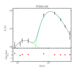
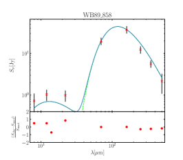
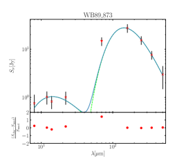
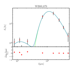
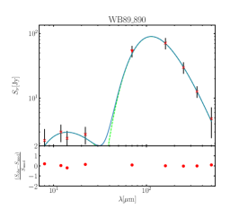
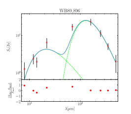
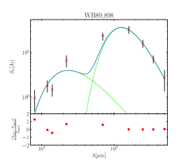
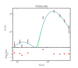
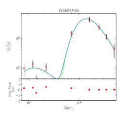
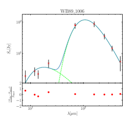
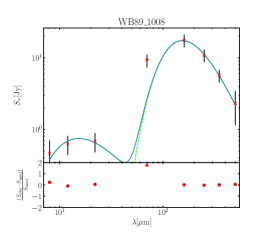
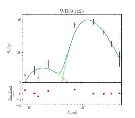
Figure 5: For each source we show the SED fit (top panel) and the residuals $(S_{\mathrm{obs}}-S_{\mathrm{mod}})/S_{\mathrm{obs}}$ (bottom panel). In the top panel, the extracted fluxes are indicated by the red crosses, and upper and lower limits are indicated by triangles pointing downwards and upwards, respectively. The best fit curve is indicated in blue, and the separate contribution of the grey- and black-body is shown by the green dashed lines. If the residuals in the bottom panel exceed —2—, the point is indicated by a triangle.

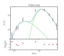
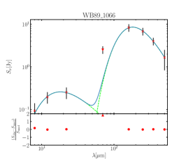
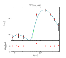
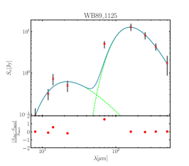
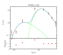
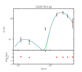
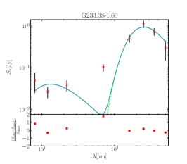
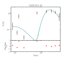
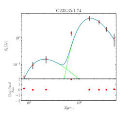
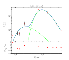
Figure 5: Continued.

The dust opacity and emissivity used are the same as in König et al. (2017), that is, $\kappa_{870\usk\mathrm{\SIUnitSymbolMicro}\mathrm{m}}=1.85\usk\mathrm{c}\mathrm{m}^{2}\usk\mathrm{g}^{-1}$ and $\beta=1.75$, respectively (see e.g. Kauffmann et al., 2008). The SEDs for the entire sample can be found in Fig. 5; an example is shown in Fig. 2. In addition to the mass surface density of dust at the far-IR peak, we derived the bolometric luminosity, the dust temperature and mass of the sources, as measured within the apertures listed in Table 1, that contains the complete results of the SED fit.

We fitted the C¹⁸O (2–1) line using MCWeeds (Giannetti et al., 2017) with the algorithm that makes use of the Normal approximation (Gelman et al., 2003) to obtain the column density of carbon monoxide, under the assumption of LTE; the adopted partition function is reported in Table 2. Using the relation between the dust temperature and the excitation temperature of CO isotopologues found in Giannetti et al. (2017, see their Fig. 10), we estimated the excitation conditions for the sources in the FOG. We used this value of $T_{\mathrm{{ex}}}$ as the most probable one in the prior, with a value of $\sigma$ equal to the measured intrinsic scatter; all priors are fully described in Table 3 and the results are listed in Table 4. To exclude biases connected to the $T_{\mathrm{{d}}}\,vs.T_{\mathrm{{ex}}}$ relation, we compared the column densities with those computed using the unmodified values of the dust temperature from the SED; this has only a minor impact on the derived quantities. In Appendix C we show the fit results, superimposed on the observed spectra; an example is given in Fig. 3.

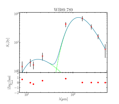
Figure 2: Top: example of the SED fit for WB$\_$789, hosting one of the the furthest clusters from the galactic centre yet detected (Brand & Wouterloot, 2007). Extracted fluxes are indicated by the red crosses, and upper and lower limits are indicated by triangles pointing downwards and upwards, respectively. The best fit curve is indicated in blue, and the separate contributions of the grey and black bodies are shown by the green dashed lines. Bottom: Residuals calculated as $(S_{\mathrm{obs}}-S_{\mathrm{mod}})/S_{\mathrm{obs}}$. The SED and their residuals for all the other sources are included in Fig. 5.

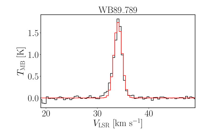
Figure 3: Example of the C¹⁸O(2–1) observations for WB$\_$789. We indicate in red the best fit from MCWeeds. The spectra and their fits for the entire sample are shown in Fig. 6.

In order to study how the gas-to-dust ratio varies across the galactic disk, we complemented the FOG sample with sources selected from the TOP100 (Giannetti et al., 2014; König et al., 2017), a representative and statistically significant sample of high-mass star-forming clumps covering a wide range of evolutionary phases (König et al., 2017; Giannetti et al., 2017). These sources are among the brightest in their evolutionary class in the inner Galaxy. For the 57 sources classified as Hii and IRb in the TOP100, we used the column density determinations from Giannetti et al. (2014) to derive the H₂ column density. Among the isotopologues analysed in that work, we elected to use C¹⁷O, because in these extreme sources C¹⁸O can have a non-negligible optical depth, and because we have FLASH⁺ (Klein et al., 2014) observations of C¹⁷O (3–2) for the entire subsample.

We have $\mathrm{C^{17}O(1-0)}$ for 17 of the selected sources in the TOP100, for which we were able to estimate the optical depth; $30\%$ of the sample has an optical depth $\approx 0.1$, the remaining clumps have optical depths below this value. Assuming LTE, $T=30\usk\mathrm{K}$, and $\tau_{\mathrm{C^{17}O(1-0)}}=0.1$, the optical depth of $\mathrm{C^{17}O(3-2)}$ is about a factor of four to five higher than that of the (1–0) transition, leading to an underestimate of the carbon monoxide column density less than $\sim 30\%$. Therefore the correction for opacity can be considered negligible (see Sect. 4). The column density of C¹⁷O is then converted to C¹⁸O using ${}^{18}\mathrm{O}/^{17}\mathrm{O}=4$, according to Giannetti et al. (2014), as determined from the same sample. The peak surface densities (and total masses) of dust for the clumps in the TOP100 were taken from the results of König et al. (2017). The properties of the sources extracted from the TOP100 are listed in Table LABEL:tab:mcweeds_fit.

We computed the mass surface density of the gas from the column density of C¹⁸O, obtained via MCWeeds for the FOG sample, and of C¹⁷O for the TOP100. When more than one velocity component was observed in the spectra of the CO isotopologues, the column densities were summed to obtain the total surface density of carbon monoxide along the line of sight, because all sources contribute to the observed continuum. This has the effect of introducing scatter in the value of $\gamma$ at a particular $R_{\mathrm{GC}}$, as the clumps have different distances, but it only happens in a minor fraction of the sources (e.g. two in the FOG sample), and depends on the $R_{\mathrm{GC}}$ of the sources. From the C¹⁸O surface density, we derived the total mass surface density of the cloud ($\Sigma$), accounting for helium, and assuming that the expected abundance of the C¹⁸O is described by:

$$\chi_{\mathrm{C^{18}O}}^{\mathrm{E}}=\frac{9.5\times 10^{-5}\times 10^{\alpha(R_{\mathrm{GC}}-R_{\mathrm{GC,\odot}})}}{{}^{16}\mathrm{O}/^{18}\mathrm{O}},$$ (1)

where $R_{\mathrm{GC}}$ is expressed in $\mathrm{kpc}$, $R_{\mathrm{GC,\odot}}=8.34\usk\mathrm{kpc}$ (Reid et al., 2014), and $\alpha$ describes the C/H gradient, taken to be $-0.08\usk\mathrm{dex}\usk\mathrm{kpc}^{-1}$ from Luck & Lambert (2011). We assumed that the CO abundance is controlled by the carbon abundance, because it is always less abundant than oxygen, and becomes progressively more so in the outer Galaxy. A smaller abundance of CO at lower $Z$ is consistent with observations of low-metallicity galaxies, where the detectable CO-emitting region is significantly smaller than the H₂ envelope (Elmegreen et al., 2013; Rubio et al., 2015). The oxygen isotopic ratio is commonly described by the relation ${}^{16}\mathrm{O}/^{18}\mathrm{O}=58.8R_{\mathrm{GC}}+37.1$ (Wilson & Rood, 1994). On the one hand, independent measurements of ${}^{16}\mathrm{OH}/^{18}\mathrm{OH}$ by Polehampton et al. (2005), despite finding consistent results with the previous works, do not strongly support such a gradient. On the other hand, Wouterloot et al. (2008) find an even steeper gradient considering sources in the FOG, where C¹⁸O is likely to be less abundant, if not for the oxygen isotopic ratio, then for selective photodissociation due to lower shielding of the dust, and self-shielding.

For the moment we ignore the effect of a gradient, and adopt the local CO/C¹⁸O ratio. We used $\Sigma$, together with $\Sigma_{\mathrm{dust}}$, as observed data for a JAGS (Just Another Gibbs Sampler, Plummer, 2003) model which derives the gas-to-dust ratios as $\Sigma/\Sigma_{dust}$, and fits the points in a log-linear space, considering an intrinsic scatter. Figure 4a shows that the gas-to-dust ratio increases with galactocentric distance, with a gradient for $\gamma\,vs.\,\ R_{\mathrm{GC}}$ described by:

$$log(\gamma)=\left(0.087\left[{}^{{+0.045}}_{{-0.025}}\right]\pm 0.007\right)\,R_{\mathrm{GC}}+\left(1.44\left[{}^{{-0.45}}_{{+0.21}}\right]\pm 0.03\right),$$ (2)

where $R_{\mathrm{GC}}$ is expressed in $\mathrm{kpc}$; we first indicate the systematic uncertainty between square brackets (discussed in the next section), and the statistical uncertainties afterwards. This equation gives values for $\gamma$ at the Sun distance between $\approx 130$ and $\approx 145$, well consistent with the local value of 136, considering the intrinsic scatter of the observed points (cf. Fig. 4) and the uncertainties in the derived relation. As indicated in Fig. 4a, our results are, in general, valid only between $\sim 2\usk\mathrm{kpc}$ and $\sim 20\usk\mathrm{kpc}$ from the galactic centre, the range spanned by the sources in our sample.

The slope of the gradient is very close to that used in Eq. 1, showing that C¹⁸O behaves in a way comparable to the dust, with respect to metallicity. This implies that the results are closely linked to the assumed galactocentric carbon gradient. In the next section we discuss as limiting cases how the $\gamma$ gradient would change if the CO abundance follows the oxygen variation instead, and if C¹⁸O is less abundant with respect to CO in the outer Galaxy, as a consequence of the ${}^{16}\mathrm{O}/^{18}\mathrm{O}$ gradient, or of selective photodissociation (see also Fig. 4b, c). The effect of such systematic uncertainties causes the variations in the slope and intercept of Eq. 2 indicated in the square brackets.

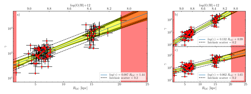
Figure 4: Variation of the gas-to-dust ratio with galactocentric radius, for our fiducial case (Panel a), considering a CO/C¹⁸O galactocentric gradient (Panel b), and assuming that the abundance of CO follows the radial oxygen gradient, rather than the C/H (Panel c). The thick blue lines indicate the best fit, reported in the bottom right corner; the $68\%$ and $95\%$ highest probability density intervals of the fit parameters are indicated by the light and dark yellow-shaded regions, respectively. The intrinsic scatter is indicated by the dashed lines. For comparison with external galaxies $log$(O/H) + 12 is shown on the top axis.

4 Discussion

In this section, we discuss the uncertainties in the gas-to-dust ratio estimates and in its galactocentric gradient, why $\gamma$ has to be higher at large $R_{\mathrm{GC}}$, and how it depends on metallicity. Estimates of the gas-to-dust ratio are difficult, resting on the derivation of surface densities of a tracer of H₂ (C¹⁸O and C¹⁷O in our case) and of the dust. Several assumptions introduce a systematic uncertainty in $\gamma$. For the surface density of molecular gas, the main sources of uncertainties are the canonical CO abundance, that can vary by a factor of two, the CO–C¹⁸O conversion, discussed in Sect. 3, and the assumption of LTE, which is likely less important, given the results of the comparison between temperatures derived from CH₃CCH and CO isotopologues in the TOP100 sample in Giannetti et al. (2017). Dust is more problematic, especially because its properties are poorly constrained. Opacity and emissivity are sensitive to the grain composition and size distribution: distinct models can induce discrepancies in the estimated mass surface density of dust up to a factor of approximately three (see e.g. Ossenkopf & Henning, 1994; Li & Draine, 2001; Gordon et al., 2014, 2017). The simple SED model adopted is a crude approximation as well: temperature varies along the line of sight, and in the extreme case where the representative grey-body temperature changes from $\approx 20\usk\mathrm{K}$ (the median in our FOG sample is $\approx 23\usk\mathrm{K}$) to $\approx 50\usk\mathrm{K}$, the dust surface density changes by a factor of approximately five.

Propagating these to the gas-to-dust ratio implies a global uncertainty of nearly a factor of six on $\gamma$ for each target. It is therefore relevant to test whether a simpler model with a constant $\gamma$ ratio is to be favoured over the proposed gradient. A Bayesian model comparison, which automatically takes into account the Ockham’s Razor principle (e.g. Bolstad, 2007), shows that, in the unfavourable case that the CO abundance follows the oxygen gradient, the odds ratio is approximately eight in favour of the gradient model, which is then to be preferred over a constant value of $\gamma$ across the entire disk.

Factors that can change the slope of the $\gamma\,vs.\,R_{\mathrm{GC}}$ relation are the molecular gas- and the CO-dark gas fractions, the CO abundance gradient, and the dust model. Larger quantities of gas in atomic form, as well as more CO-dark gas at lower metallicities (due to a lower shielding of dust and self-shielding) would cause the relation to be steeper. However, because we target exclusively dense molecular clouds, the vast majority of gas should be in molecular form (see Sect. 2). A larger fraction of CO-dark gas is evident for the low-metallicity galaxy WLM (Elmegreen et al., 2013; Rubio et al., 2015); a less extreme, but analogous situation is possible for clouds at the edge of the Milky Way disk (in the FOG, $Z$ is larger than in WLM by a factor of between approximatley two and five, see Leaman et al., 2012).

On the other hand, the variation of dust composition and size distribution of grains tend to make the measured relation flatter. Silicates are likely to be more common in the outer Galaxy (e.g. Carigi et al., 2005); in this case the opacity would be lower, leading to an underestimate of the dust surface density. The models in Ossenkopf & Henning (1994) show that a variation in the silicate-to-carbon fraction has a much smaller impact than the change in size distribution due to coagulation. In the extreme case in which no coagulation takes place in the FOG, and it is, on the contrary, efficient in the inner Galaxy, the dust opacity changes by a factor of approximately two in the far-IR and submm regimes, reducing the mass surface densities by the same quantity. This effect has an impact similar in magnitude, but opposite, to that of the CO/C¹⁸O gradient.

In the outer Galaxy, where extinction is lower, dust grains can be more efficiently reprocessed. As a consequence, more carbon is present in the gas phase (e.g. Parvathi et al., 2012), effectively making the gradient in CO abundance shallower than the C/H one, if it follows the gas-phase abundance of carbon. A limiting case is obtained by using the slope of the oxygen gradient in Eq. 1, in which case the slope in Eq. 2 can be as shallow as $0.062\usk\mathrm{dex}\usk\mathrm{kpc}^{-1}$. It is, however, unlikely that the increased abundance of C in the gas phase and the less efficient coagulation have such an important effect. Conversely, if we neglect these effects, but consider the CO/C¹⁸O gradient, we can obtain an upper limit for the gradient slope. Under these conditions, $\gamma$ varies by $0.132\usk\mathrm{dex}\usk\mathrm{kpc}^{-1}$.

The CO/C¹⁸O abundance gradient, and larger fractions of CO-dark and atomic gas at lower metallicity (see e.g. Elmegreen et al., 2013; Rubio et al., 2015) contrast the effects of the increased fraction of C in the gas phase, of dust size distribution and composition. For simplicity, as a fiducial value, we have therefore considered the relation for which the variation in grain size distribution and the increased fraction of CO-dark gas cancel out the impact of the CO/C¹⁸O abundance gradient (Fig. 4a).

Theoretical considerations also indicate that the gas-to-dust ratio has to be higher in the FOG. In the following, we show that at a distance of $\sim 15\usk\mathrm{kpc}$ the fraction of heavy elements locked into dust grains must be $80\%$ to maintain $\gamma$ at the local value of $136$. Following Mattsson & Andersen (2012) we can conservatively use the O/H gradient to obtain an approximation of the galactocentric metallicity behaviour. The radial $Z$ gradient for our Galaxy can be reliably obtained via measurements of the abundance of heavy elements in Cepheids, which are young enough to represent the present-day composition. We use the results from Luck & Lambert (2011), who consider a large number of Cepheids with $5\usk\mathrm{kpc}\lesssim R_{\mathrm{GC}}\lesssim 17\usk\mathrm{kpc}$, deriving for oxygen the gradient $d\mathrm{[O/H]}/dR_{\mathrm{GC}}=-0.056\,\mathrm{dex}\usk\mathrm{kpc}^{-1}$. We obtain for $Z$:

$$log(Z)=-0.056R_{\mathrm{GC}}-1.176,$$ (3)

which gives, at the location of the Sun, an H-to-metal mass ratio $\sim 44$. If approximately $40\%$ of the heavy elements are locked into dust grains (Dwek, 1998), this implies $\gamma=110$, which is in very good agreement with the locally-estimated value of $136$.

The dust-to-gas mass ratio $Z_{d}$ is the inverse of $\gamma$, and the fraction of mass in heavy elements locked in dust grains, the dust-to-metal ratio, can be expressed as the ratio of $Z_{d}$ and the gas metallicity, that is, $Z_{d}/Z$. A dust-to-metal ratio of one would imply that dust grains contain all elements heavier than helium. If we were to assume that the gas-to-dust ratio remains constant to $\gamma\equiv Z_{d}^{-1}=136$ (implying that progressively more heavy elements end up in dust grains), using Eq. 3 we would see that the dust metallicity $Z_{d}/Z$ reaches $80\%$ at $R_{\mathrm{GC}}\approx 15\usk\mathrm{kpc}$. In addition, the metallicity gradient is most likely steeper than the oxygen gradient (e.g. Mattsson & Andersen, 2012), moving this limit inwards, thus indicating that in the FOG the gas-to-dust ratio is bound to be higher.

Now using our results for the increase of the gas-to-dust ratio with $R_{\mathrm{GC}}$, the dust metallicity can be derived from Eqs. 2 and 3:

$$log\left(\frac{Z_{d}}{Z}\right)=\left(-0.031\left[{}^{{+0.025}}_{{-0.047}}\right]\right)R_{\mathrm{GC}}-\left(0.26\left[{}^{{-0.21}}_{{+0.45}}\right]\right),$$ (4)

which shows that the dust-to-metal ratio decreases with galactocentric radius. A decrease of the the dust-to-metal ratio is the most common situation in late-type galaxies and indicates that grain growth in the dense ISM dominates over dust destruction (e.g. Mattsson & Andersen, 2012; Mattsson et al., 2014). This strongly reinforces the previous argument that a constant $\gamma=136$ cannot be sustained in the far outer Galaxy, because the metal-to-dust ratio virtually always decreases moving outwards in the disk, for Milky-Way type galaxies.

A good test bench for Eq. 2 is represented by the Magellanic Clouds. Combining Eqs. 2 and 3, and using the appropriate metallicity ($Z=0.5\,Z_{\odot}$ and $Z=0.2\,Z_{\odot}$ for the Large and Small Magellanic Clouds, respectively; Russell & Dopita, 1992), we obtain $\gamma\sim 420^{{+250}}_{{-110}}$ and $\gamma=1750^{{+4100}}_{{-900}}$, in excellent agreement with the results of Roman-Duval et al. (2014).

5 Summary and conclusions

We combined our molecular-line surveys towards dense and massive molecular clouds in the inner- and far outer disk of the Milky Way to study how the gas-to-dust ratio $\gamma$ varies with galactocentric distance and metallicity. We estimated conservative limits for the galactocentric gradient of gas-to-dust mass ratio, by considering multiple factors that influence its slope (see Sect. 4), and defined, for simplicity, the fiducial value as the case where dust coagulation and the larger fraction of carbon in the gas phase in the FOG balance the CO/C¹⁸O abundance gradient. The gas-to-dust mass ratio is shown to increase with $R_{\mathrm{GC}}$ according to Eq. 2, and this gradient is compared with that of metallicity, as obtained from Cepheids by Luck & Lambert (2011). The variation in gas-to-dust ratio is steeper than that of $Z$ ($\gamma\propto Z^{-1.4^{{+0.3}}_{{-1.0}}}$), implying that the the dust-to-metal ratio decreases with distance from the galactic centre. This indicates that dust condensation in the dense ISM dominates over dust destruction, which is typical of late-type galaxies like ours (Mattsson & Andersen, 2012; Mattsson et al., 2014). The predictions obtained combining Eq. 2 and 3 for the metallicities of the Magellanic Clouds are in excellent agreement with the results on $\gamma$ in these galaxies by Roman-Duval et al. (2014).

The use of Eq. 2 to calculate the appropriate value of $\gamma$ at each galactocentric radius is fundamental for the study of individual objects, allowing us to derive accurate H₂ column densities and total masses from dust continuum observations, as well as for any study that compares the properties of molecular clouds in the inner and outer Galaxy. This opens the way for a complete view of the galactic disk and of the influence of $Z$ on the physics and chemistry of molecular clouds.

Appendix A Tables

Table 1: Properties of the sources and results of the SED fit procedure for the far outer Galaxy sample.

Source	$l$	$b$	Dist.	$R_{\mathrm{GC}}$	Diam.	$T_{\mathrm{{d}}}$	$L_{bol}$	$M_{dust}$	$\Sigma_{dust}$
	deg	deg	[kpc]	[kpc]	$[\arcsec]$	[K]	$[10^{x}\usk\mathrm{L_{\odot}}]$	$[10^{x}\usk\mathrm{M_{\odot}}]$	$[10^{x}\usk\mathrm{g}\usk\mathrm{c}\mathrm{m}^{-2}]$
WB89_898	$217.604$	$-2.617$	8.8	16.4	109	$24.1\pm 5.7$	$3.65\pm 0.24$	$0.15\pm 0.19$	$-3.84\pm 0.19$
WB89_986	$229.772$	$0.060$	7.9	14.9	120	$22.0\pm 4.7$	$3.48\pm 0.28$	$0.35\pm 0.18$	$-4.04\pm 0.18$
WB89_909	$217.331$	$-1.369$	6.3	14.0	120	$20.6\pm 2.6$	$3.72\pm 0.20$	$0.77\pm 0.13$	$-3.42\pm 0.13$
WB89_1024	$238.959$	$-1.684$	9.2	15.4	107	$24.3\pm 4.4$	$3.58\pm 0.18$	$0.04\pm 0.15$	$-4.04\pm 0.15$
WB89_890	$212.282$	$-0.617$	6.4	14.3	120	$27.2\pm 2.2$	$3.69\pm 0.13$	$0.02\pm 0.10$	$-4.23\pm 0.10$
WB89_858	$213.192$	$-3.325$	6.9	14.8	91	$25.5\pm 0.4$	$3.37\pm 0.05$	$-0.22\pm 0.09$	$-4.22\pm 0.08$
WB89_1125	$256.151$	$-1.375$	9.7	14.3	76	$19.5\pm 1.8$	$3.09\pm 0.13$	$0.22\pm 0.11$	$-4.01\pm 0.11$
WB89_879	$214.931$	$-2.719$	6.9	14.7	99	$26.5\pm 5.9$	$3.42\pm 0.29$	$-0.19\pm 0.17$	$-4.26\pm 0.17$
WB89_896	$215.888$	$-2.010$	7.9	15.6	108	$23.7\pm 4.4$	$3.50\pm 0.16$	$-0.07\pm 0.16$	$-4.18\pm 0.16$
WB89_856	$213.098$	$-3.561$	7.7	15.6	114	$26.3\pm 2.3$	$3.79\pm 0.15$	$0.24\pm 0.11$	$-4.07\pm 0.10$
WB89_1126	$257.508$	$-2.252$	10.6	15.0	53	$24.4\pm 6.8$	$3.30\pm 0.31$	$-0.15\pm 0.21$	$-4.11\pm 0.21$
WB89_1006	$235.686$	$-1.246$	8.1	14.7	110	$28.5\pm 5.3$	$3.99\pm 0.27$	$0.24\pm 0.15$	$-3.95\pm 0.15$
WB89_1008	$236.999$	$-1.838$	8.8	15.2	114	$19.8\pm 0.7$	$3.19\pm 0.06$	$0.24\pm 0.09$	$-4.05\pm 0.08$
WB89_789	$195.820$	$-0.567$	12.0	20.3	109	$23.2\pm 3.1$	$4.09\pm 0.20$	$0.81\pm 0.13$	$-3.56\pm 0.13$
WB89_1066	$245.103$	$-0.993$	9.8	15.4	87	$16.9\pm 0.2$	$2.85\pm 0.03$	$0.35\pm 0.08$	$-3.91\pm 0.08$
WB89_1023	$238.772$	$-1.810$	10.3	16.4	54	$24.6\pm 5.0$	$3.09\pm 0.28$	$-0.31\pm 0.17$	$-4.30\pm 0.16$
WB89_1080	$249.599$	$-2.075$	13.1	17.9	120	$21.8\pm 0.6$	$3.81\pm 0.05$	$0.67\pm 0.08$	$-4.25\pm 0.08$
WB89_873	$215.599$	$-3.414$	7.1	14.9	114	$21.2\pm 1.4$	$3.22\pm 0.10$	$0.12\pm 0.10$	$-4.18\pm 0.10$
G237.32–1.28	$237.320$	$-1.280$	8.7	15.1	114	$31.4\pm 11.8$	$4.51\pm 0.42$	$0.50\pm 0.23$	$-3.80\pm 0.23$
G233.38–1.60	$233.380$	$-1.600$	8.7	15.4	120	$12.1\pm 1.0$	$1.82\pm 0.09$	$-0.04\pm 0.13$	$-4.53\pm 0.13$
G229.76–0.44	$229.760$	$-0.440$	8.4	15.3	120	$13.9\pm 0.4$	$2.13\pm 0.05$	$-0.01\pm 0.09$	$-4.54\pm 0.09$
G235.35–1.74	$235.350$	$-1.690$	9.3	15.8	120	$18.1\pm 0.3$	$2.61\pm 0.04$	$-0.04\pm 0.08$	$-4.53\pm 0.08$
G233.76–1.25	$233.760$	$-1.250$	8.7	15.3	117	$13.9\pm 3.7$	$2.38\pm 0.15$	$-0.03\pm 0.27$	$-4.49\pm 0.27$

Table 2: Measurements of the C¹⁸O rotational partition function.

Temperatures [K]	9.375	18.75	37.5	75	150	225	300
Q(C18O)	3.9	7.5	14.6	28.8	57.3	85.8	114.3

Table 3: Priors used in MCWeeds.

C18O	Temperature	Column density	Linewidth	Velocity
	[K]	[log(cm-2)]	[$\mathrm{k}\mathrm{m}\usk\mathrm{s}^{-1}$]	[$\mathrm{k}\mathrm{m}\usk\mathrm{s}^{-1}$]
Prior	Truncated normal	Normal	Truncated normal	Normal
Parameters (cool)	$\mu=T_{ex,CO}$	$\mu=14$	$\mu=1$	$\mu=V_{\mathrm{{LSR}}}$
	$\sigma=15$	$\sigma=1.5$	$\sigma=1$	$\sigma=2$
	$low=7,high=100$		$low=0.3,high=6$

Table 4: Column densities, expected C¹⁸O abundances, gas-to-dust ratios and radial velocities for the far outer Galaxy sample.

Source	$N_{\mathrm{C^{18}O}}$	$\chi^{E\,}_{C^{18}O}$	$\gamma$	$\gamma_{bf}$	$N_{\mathrm{H_{2}}}$	$V_{\mathrm{{LSR}}}$
	$[10^{x}\usk\mathrm{c}\mathrm{m}^{-2}]$	[$10^{-8}$]			$[10^{22}\usk\mathrm{c}\mathrm{m}^{-2}]$	$[\mathrm{k}\mathrm{m}\usk\mathrm{s}^{-1}]$
WB89_898	$15.14\pm 0.06$	$3.8^{{+2.2}}_{{-1.7}}$	$1168^{{+923}}_{{-421}}$	$739^{{+811}}_{{-273}}$	$1.7^{{+1.8}}_{{-0.6}}$	63.35
WB89_986	$14.71\pm 0.04$	$5.0^{{+2.2}}_{{-2.0}}$	$518^{{+328}}_{{-158}}$	$547^{{+429}}_{{-171}}$	$0.8^{{+0.6}}_{{-0.2}}$	70.57
WB89_909	$15.83\pm 0.08$	$5.9^{{+2.2}}_{{-2.1}}$	$1405^{{+758}}_{{-379}}$	$458^{{+284}}_{{-127}}$	$2.7^{{+1.7}}_{{-0.8}}$	50.06/52.40a
WB89_1024	$14.88\pm 0.08$	$4.6^{{+2.2}}_{{-1.9}}$	$852^{{+583}}_{{-276}}$	$603^{{+531}}_{{-200}}$	$0.9^{{+0.8}}_{{-0.3}}$	82.42
WB89_890	$14.55\pm 0.09$	$5.6^{{+2.2}}_{{-2.0}}$	$497^{{+284}}_{{-140}}$	$486^{{+327}}_{{-141}}$	$0.5^{{+0.3}}_{{-0.1}}$	46.29/47.59a
WB89_858	$14.78\pm 0.09$	$5.2^{{+2.2}}_{{-2.0}}$	$902^{{+555}}_{{-269}}$	$529^{{+397}}_{{-162}}$	$0.5^{{+0.4}}_{{-0.2}}$	49.34
WB89_1125	$14.79\pm 0.04$	$5.6^{{+2.2}}_{{-2.0}}$	$535^{{+306}}_{{-151}}$	$488^{{+330}}_{{-142}}$	$0.7^{{+0.5}}_{{-0.2}}$	86.08
WB89_879	$14.04\pm 0.12$	$5.2^{{+2.2}}_{{-2.0}}$	$179^{{+109}}_{{-53}}$	$525^{{+390}}_{{-160}}$	$0.4^{{+0.3}}_{{-0.1}}$	51.98
WB89_896	$14.59\pm 0.08$	$4.5^{{+2.2}}_{{-1.8}}$	$618^{{+435}}_{{-204}}$	$627^{{+576}}_{{-213}}$	$0.6^{{+0.6}}_{{-0.2}}$	57.55
WB89_856	$15.01\pm 0.09$	$4.5^{{+2.2}}_{{-1.8}}$	$1246^{{+872}}_{{-410}}$	$622^{{+567}}_{{-210}}$	$0.8^{{+0.8}}_{{-0.3}}$	52.63
WB89_1126	$14.80\pm 0.08$	$5.0^{{+2.2}}_{{-2.0}}$	$768^{{+489}}_{{-235}}$	$551^{{+436}}_{{-173}}$	$0.7^{{+0.5}}_{{-0.2}}$	90.41
WB89_1006	$14.67\pm 0.10$	$5.3^{{+2.2}}_{{-2.0}}$	$367^{{+222}}_{{-108}}$	$519^{{+381}}_{{-157}}$	$0.9^{{+0.7}}_{{-0.3}}$	74.81
WB89_1008	$14.52\pm 0.04$	$4.8^{{+2.2}}_{{-1.9}}$	$365^{{+244}}_{{-116}}$	$584^{{+496}}_{{-190}}$	$0.8^{{+0.7}}_{{-0.3}}$	80.41
WB89_789	$15.38\pm 0.07$	$1.9^{{+1.8}}_{{-1.0}}$	$2135^{{+2555}}_{{-1032}}$	$1604^{{+3511}}_{{-795}}$	$7.0^{{+15.3}}_{{-3.5}}$	34.24
WB89_1066	$14.77\pm 0.04$	$4.6^{{+2.2}}_{{-1.9}}$	$488^{{+333}}_{{-158}}$	$602^{{+529}}_{{-200}}$	$1.2^{{+1.0}}_{{-0.4}}$	87.01
WB89_1023	$14.65\pm 0.08$	$3.9^{{+2.2}}_{{-1.7}}$	$1068^{{+839}}_{{-383}}$	$733^{{+798}}_{{-270}}$	$0.6^{{+0.6}}_{{-0.2}}$	88.74
WB89_1080	$14.36\pm 0.06$	$2.9^{{+2.0}}_{{-1.4}}$	$658^{{+624}}_{{-271}}$	$1000^{{+1470}}_{{-422}}$	$0.9^{{+1.3}}_{{-0.4}}$	105.92
WB89_873	$14.20\pm 0.06$	$5.1^{{+2.2}}_{{-2.0}}$	$218^{{+137}}_{{-66}}$	$545^{{+425}}_{{-170}}$	$0.6^{{+0.4}}_{{-0.2}}$	53.65
G237.32–1.28	$15.01\pm 0.10$	$4.9^{{+2.2}}_{{-1.9}}$	$614^{{+397}}_{{-190}}$	$563^{{+456}}_{{-179}}$	$1.4^{{+1.1}}_{{-0.4}}$	78.07
G233.38–1.60	$13.67\pm 1.30$	$4.7^{{+2.2}}_{{-1.9}}$	$157^{{+107}}_{{-51}}$	$597^{{+520}}_{{-197}}$	$0.3^{{+0.2}}_{{-0.1}}$	76.70
G229.76–0.44	$13.98\pm 0.93$	$4.7^{{+2.2}}_{{-1.9}}$	$330^{{+222}}_{{-105}}$	$592^{{+509}}_{{-194}}$	$0.3^{{+0.2}}_{{-0.1}}$	73.03
G235.35–1.74	$14.42\pm 0.14$	$4.3^{{+2.2}}_{{-1.8}}$	$953^{{+686}}_{{-320}}$	$646^{{+614}}_{{-223}}$	$0.3^{{+0.3}}_{{-0.1}}$	80.98
G233.76–1.25	$14.23\pm 0.65$	$4.7^{{+2.2}}_{{-1.9}}$	$517^{{+350}}_{{-166}}$	$595^{{+516}}_{{-196}}$	$0.3^{{+0.3}}_{{-0.1}}$	76.91

Appendix B Spectral energy distributions

Appendix C Spectra for sources in the far outer Galaxy

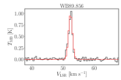
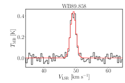
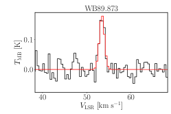
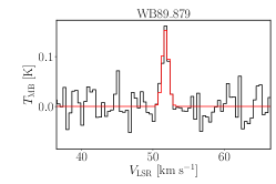
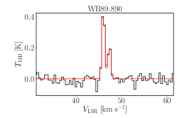
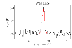
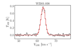
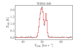
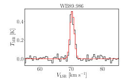
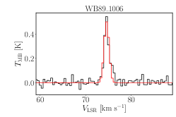
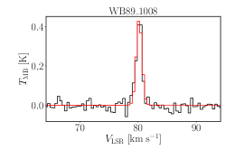
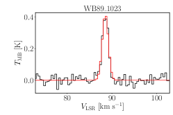
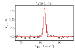
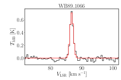
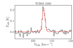
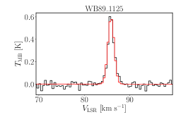
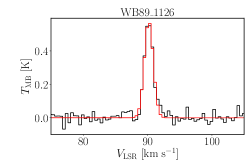
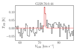
Figure 6: C¹⁸O spectra of the sources in the FOG. We show in red the best fit from MCWeeds.

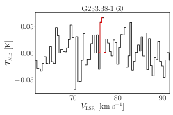
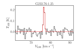
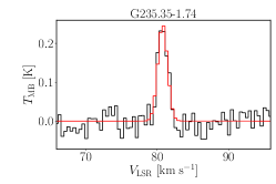
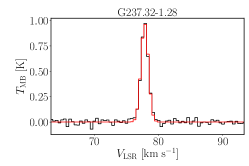
Figure 6: Continued.