Influence of $f(R)$ Models on the Existence of Anisotropic Self-Gravitating Systems

Abstract

This paper aims to explore some realistic configurations of anisotropic spherical structures in the background of metric $f(R)$ gravity, where $R$ is the Ricci scalar. The solutions obtained by Krori and Barua are used to examine the nature of particular compact stars with three different modified gravity models. The behavior of material variables is analyzed through plots and the physical viability of compact stars is investigated through energy conditions. We also discuss the behavior of different forces, equation of state parameter, measure of anisotropy and Tolman-Oppenheimer-Volkoff equation in the modeling of stellar structures. The comparison from our graphical representations may provide evidences for the realistic and viable $f(R)$ gravity models at both theoretical and astrophysical scale.

1 Introduction

General relativity (GR) laid down the foundations of modern cosmology. The observational ingredients of $\Lambda$-cold dark matter model is found to be compatible with all cosmological outcomes but suffers some discrepancies like cosmic coincidence and fine-tuning [1]. The accelerated expansion of the universe is strongly manifested after the discovery of unexpected reduction in the detected energy fluxes coming from cosmic microwave background radiations, large scale structures, redshift and Supernovae Type Ia surveys [2]. These observations have referred dark energy (DE) (an enigmatic force), a reason behind this interesting and puzzling phenomenon. Various techniques have been proposed in order to modify Einstein gravity in this directions. Qadir et al. [3] discussed various aspects of modified relativistic dynamics and proposed that GR may need to modify to resolve various cosmological issues, like quantum gravity and dark matter problem.

The modified theories of gravity are the generalized models came into being by modifying only the gravitational portion of the GR action (for further reviews on DE and modified gravity, see, for instance, [4, 5, 6, 7, 8, 9, 10, 11, 12, 13, 14, 15, 16]). The first theoretical and observationally viable possibility of our accelerating cosmos from $f(R)$ gravity was proposed by Nojiri and Odintsov [17]. There has been interesting discussion of dark cosmic contents on the structure formation and the dynamics of various celestial bodies in Einstein-$\Lambda$ [18], $f(R)$ [19], $f(R,T)$ [20] ($T$ is the trace of energy momentum tensor) and $f(R,T,R_{\mu\nu}T^{\mu\nu})$ gravity [21]. Recently, Nojiri et al. [22] have studied variety of cosmic issues, like early-time, late-time cosmic acceleration, bouncing cosmology. They emphasized that some extended gravity theories such as $f(R),~{}f(G)$ (where $G$ is the Gauss-Bonnet term) and $f(\mathcal{T})$ (where $\mathcal{T}$ is the torsion scalar) can be modeled to unveil various interesting cosmic scenarios.

The search for the effects of anisotropicity in the matter configurations of compact objects is the basic key leading to various captivating phenomena, like transitions of phase of different types [23], condensation of pions [24], existence of a solid as well as Minkowskian core [25, 26] etc. One can write all possible exact solutions of static isotropic relativistic collapsing cylinder in terms of scalar expressions in GR [27] as well as in $f(R)$ gravity [28]. Sussman and Jaime [29] analyzed a class of irregular spherical solutions in the presence of a specific traceless anisotropic pressure tensor for the choice of $f(R)\propto\sqrt{R}$ model. Shabani and Ziaie [30] used dynamical and numerical techniques to analyze the effects of a particular $f(R,T)$ gravity model on the stability of emergent Einstein universe. Garattini and Mandanici [31] examined some stable configurations of various anisotropic relativistic compact objects and concluded that extra curvature gravitational terms coming from rainbow’s gravity likely to support various patterns of compact stars. Sahoo and his collaborators [32] explored various cosmological aspects in the context anisotropic relativistic backgrounds.

Gravitational collapse (GC) is an interesting process, due to which the stellar bodies could gravitate continuously to move towards their central points. In this regard, the singularity theorem [33] states that during this implosion process of massive relativistic structures, the spacetime singularities may appear in the realm of Einstein’s gravity. The investigation of the final stellar phase has been a source of great interest for many relativistic astrophysicists and gravitational theorists. In this respect, various authors [34] explored the problem of GC by taking some realistic configurations of matter and geometry. In the context of $f(R)$ gravity, various results have been found in literature about collapsing stellar interiors and black holes [35].

Capozziello et al. [36] studied GC of non-interacting particles by evaluating dispersion expressions through perturbation approach and found some unstable regime of the collapsing object under certain limits. Cembranos et al. [37] examined GC of non-static inhomogeneous gravitational sources and studied the large-scale structure formation at early-time cosmic in different $f(R)$ gravity theories. Modified gravity theories likely to host massive celestial objects with smaller radii as compared to GR [38]. Guo and Joshi [39] discussed scalar GC of spherically symmetric spacetime and inferred that relativistic sphere could give rise to black hole configurations, if the source field is strong.

The concept of energy conditions (ECs) could be considered as viable approach for the better understanding of the well-known singularity theorem. Santos et al. [40] developed viability bounds coming from ECs on generic $f(R)$ formalism. Their approach could be considered to constrain various possible $f(R)$ gravity models with proper physical backgrounds. Wang et al. [41] evaluated some generic expressions for ECs in the $f(R)$ gravity and employed them on a class of cosmological model to obtain some viability constraints.

Shiravand et al. [42] evaluated ECs for $f(R)$ gravity and obtained some stability constraints against Dolgov-Kawasaki instability. They found special ranges of some $f(R)$ model parameters under which the theory would satisfy WECs. The investigation of ECs in modified theories has been carried out under a variety of cosmological issues like, $f(R)$ gravity [43], $f(R,L_{m})$ gravity [44], $f(R,T)$ gravity [45], $f(R,G)$ gravity [46], $f(G)$ gravity [47]. The stability of compact objects along with their ECs have been analyzed in detail by various researchers [48].

The main goal of this paper is to investigate the role of $f(R)$ models as well as anisotropic pressure in the modeling of realistic compact stellar structures. We study various structural properties, like distributions of density and pressure anisotropicity, Tolman-Oppenheimer-Volkoff (TOV) equation, energy conditions, stability as well as equation of state parameter, for three different observational data of stellar structures. The paper is outlined as follows. In the next section, we briefly review $f(R)$ gravity for anisotropic configurations of the static spherical geometry. Section 3 is devoted to demonstrate some $f(R)$ gravity models along with their physical viability. In section 4, we check physical viability of three well-known stellar structure. At the end, we conclude our main findings.

2 Anisotropic Relativistic Spheres in $f(R)$ Gravity

The standard Einstein-Hilbert action in $f(R)$ gravity can be modified as follows

$$S_{f(R)}=\frac{1}{2\kappa}\int d^{4}x\sqrt{-g}f(R)+S_{M},$$ (1)

where $g,~{}\kappa,~{}S_{M}$ stand for the determinant of the tensor, the coupling constant and matter field action. The basic motivation of this theory is to introduce generic algebraic expression of the Ricci scalar rather than cosmological constant in the GR action. By giving variation in the above equation with respect to $g_{\mu\nu}$, the field equations for $f(R)$ gravity can be found as

$$R_{\alpha\beta}f_{R}-\frac{1}{2}f(R)g_{\alpha\beta}+\left(g_{\alpha\beta}{\Box}-\nabla_{\alpha}\nabla_{\beta}\right)f_{R}={\kappa}T_{\alpha\beta},$$ (2)

where $T_{\alpha\beta}$ is the standard energy-momentum tensor, while $\nabla_{\beta}$ is an operator of covariant derivative, $\Box\equiv\nabla^{\beta}\nabla_{\beta}$ and $f_{R}\equiv df/dR$. The quantity $f_{R}$ comprises of second corresponding derivatives of the metric variables, which is often termed as scalaron which propagates new scalar freedom degrees. The trace of Eq.(2) specifies scalaron equation of motion as under

$$3\Box{f_{R}}+{R}f_{R}-2f(R)={\kappa}T,$$ (3)

where $T\equiv T^{\beta}_{\beta}$. It has been noticed that above equation is a second order differential equation in $f_{R}$, unlike GR in which the trace of Einstein field equation boils down to $R=-\kappa T$. This points $f_{R}$ as a source of producing scalar degrees of freedom in $f(R)$ theory. The condition $T=0$ does not necessarily implies the vanishing (or constant value) of the Ricci scalar in the dynamics. This presents Eq.(3) as a useful mathematical tool to discuss many hidden and interesting cosmic arena, like Newtonian limit, stability etc. The constraint, constant Ricci scalar as well as $T_{\alpha\beta}=0$, boil down Eq.(3) as

$$Rf_{R}-2f(R)=0,$$ (4)

which is the Ricci algebraic equation after choosing any viable formulations of $f(R)$ model. If someone finds a constant roots of the above equation, i.e., $R=\Lambda$ (say), then Eq.(3) yields

$$R_{\alpha\beta}=\frac{g_{\alpha\beta}\Lambda}{4},$$ (5)

thereby indicating (anti) de Sitter as the maximally symmetric solution. Equation (2) can be remanipulated as

$$G_{\alpha\beta}=\frac{\kappa}{f_{R}}(\overset{(D)}{T_{\alpha\beta}}+T_{\alpha\beta})\equiv{T_{\alpha\beta}^{\textrm{eff}}},$$ (6)

where $G_{\alpha\beta}$ is an Einstein tensor and $\overset{(D)}{T_{\alpha\beta}}$ is termed as effective form of the energy-momentum tensor. Its expression is given by

$$\overset{(D)}{T_{\alpha\beta}}=\frac{1}{\kappa}\left\{\nabla_{\alpha}\nabla_{\beta}f_{R}-\Box f_{R}g_{\alpha\beta}+(f-Rf_{R})\frac{g_{\alpha\beta}}{2}\right\}.$$

We consider a general form of a static spherically symmetric line element as

$$d{s^{2}}=e^{a}d{t^{2}}-e^{b}d{r^{2}}-{r^{2}}({d{\theta^{2}}+{{r^{2}}{\sin}^{2}}\theta d{\phi^{2}}}),$$ (7)

where $a$ and $b$ are radial dependent metric coefficients. We assume that our spherical self-gravitating system is filled with locally anisotropic relativistic fluid distributions. The energy-momentum tensor of this matter is given by

$${T_{\mu\nu}}=(\rho+p_{t}){U_{\mu}}{U_{\nu}}-{p_{t}}{g_{\mu\nu}}+({p_{r}}-{p_{t}}){V_{\mu}}{V_{\nu}},$$ (8)

where $p_{r},~{}p_{t}$ are the radial and tangential components of pressure and $\rho$ is the fluid energy density. The four-vectors $U_{\mu}$ and $V_{\mu}$, under non-tilted coordinate frame, obey relations $U_{\mu}U^{\mu}=1$ and $V_{\mu}V^{\mu}=-1$. The $f(R)$ field equations (6) for the metric (7) and fluid (8) can be given as

$$\rho =\frac{{{e^{-b}}}}{{2{r^{2}}}}({r^{2}}b^{\prime}{f_{R}}^{\prime}+2{f_{R}}rb^{\prime}+f(-{r^{2}}{e^{b}})+{f_{R}}{r^{2}}{e^{b}}R+2{f_{R}}{e^{b}}-2{r^{2}}{f_{R}}^{\prime\prime}$$

$$-4r{f_{R}}^{\prime}-2{f_{R}}),$$ (9)

$${p_{r}} =-\frac{{{{\rm{e}}^{-b}}}}{{2{r^{2}}}}(-2{f_{R}}+2{{\rm{e}}^{b}}{f_{R}}-{{\rm{e}}^{b}}f{r^{2}}+{{\rm{e}}^{b}}{f_{R}}{r^{2}}R-2{f_{R}}ra^{\prime}-4r{f_{R}}^{\prime}-{r^{2}}a^{\prime}{f_{R}}^{\prime}),$$ (10)

$${p_{t}} =\frac{{{e^{-b}}}}{{4r}}(2{f_{R}}ra^{\prime\prime}-{f_{R}}ra^{\prime}b^{\prime}+2ra^{\prime}{f_{R}}^{\prime}+{f_{R}}r{{a^{\prime}}^{2}}+2{f_{R}}a^{\prime}-2rb^{\prime}{f_{R}}^{\prime}-2{f_{R}}b^{\prime}$$

$$+2rf{e^{b}}-2r{f_{R}}{e^{b}}R+4r{f_{R}}^{\prime\prime}+4{f_{R}}^{\prime}).$$ (11)

The corresponding Ricci scalar is given by

$$R=\frac{{{{\rm{e}}^{-b}}}}{{2{r^{2}}}}\left[4-4{{\rm{e}}^{b}}+{r^{2}}{a^{\prime 2}}-4rb^{\prime}+ra^{\prime}\left({4-rb^{\prime}}\right)+2{r^{2}}{a^{\prime\prime}}\right].$$ (12)

In order to achieve some realistic study for the modeling of anisotropic compact stellar structure, we use a specific combination of metric variables, i.e., $a(r)=Br^{2}+C$ and $b(r)=Ar^{2}$ suggested by Krori and Barua [49]. Here, $A,~{}B$ and $C$ are constants and can be found by imposing some viable physical grounds. Making use of these expressions, the $f(R)$ field equations can be recasted as

$$\rho =\frac{1}{{2{r^{2}}}}{{\rm{e}}^{-{r^{2}}A}}(-2{f_{R}}+2{{\rm{e}}^{{r^{2}}A}}{f_{R}}-{{\rm{e}}^{{r^{2}}A}}f{r^{2}}+4{f_{R}}{r^{2}}A+{{\rm{e}}^{{r^{2}}A}}{f_{R}}{r^{2}}R+2{f_{R}}{r^{3}}A^{\prime}-4r{f_{R}}^{\prime}$$

$$+2{r^{3}}A{f_{R}}^{\prime}+{r^{4}}A^{\prime}{f_{R}}^{\prime}-2{r^{2}}{f_{R}}^{\prime\prime}),$$ (13)

$${p_{r}} =-\frac{1}{{2{r^{2}}}}{{\rm{e}}^{-{r^{2}}A}}(-2{f_{R}}+2{{\rm{e}}^{{r^{2}}A}}{f_{R}}-{{\rm{e}}^{{r^{2}}A}}f{r^{2}}-4{f_{R}}{r^{2}}B+{{\rm{e}}^{{r^{2}}A}}{f_{R}}{r^{2}}R-2{f_{R}}{r^{3}}B^{\prime}$$

$$-4r{f_{R}}^{\prime}-2{r^{3}}B{f_{R}}^{\prime}-{r^{4}}B^{\prime}{f_{R}}^{\prime}),$$ (14)

$${p_{t}} =\frac{1}{{4r}}{{\rm{e}}^{-{r^{2}}A}}(2{{\rm{e}}^{{r^{2}}A}}fr-4{f_{R}}rA+8{f_{R}}rB-4{f_{R}}{r^{3}}AB+4{f_{R}}{r^{3}}{B^{2}}-2{{\rm{e}}^{{r^{2}}A}}{f_{R}}rR-2{f_{R}}{r^{2}}$$

$$\times A^{\prime}-2{f_{R}}{r^{4}}BA^{\prime}+10{f_{R}}{r^{2}}B^{\prime}-2{f_{R}}{r^{4}}AB^{\prime}+4{f_{R}}{r^{4}}BB^{\prime}-{f_{R}}{r^{5}}A^{\prime}B^{\prime}+{f_{R}}{r^{5}}{{B^{\prime}}^{2}}+4{f_{R}}^{\prime}$$

$$-4{r^{2}}A{f_{R}}^{\prime}+4{r^{2}}B{f_{R}}^{\prime}-2{r^{3}}A^{\prime}{f_{R}}^{\prime}+2{r^{3}}B^{\prime}{f_{R}}^{\prime}+2{f_{R}}{r^{3}}{B^{\prime\prime}}+4r{f_{R}}^{\prime\prime}).$$ (15)

Now, we consider a three-dimensional hypersurface, $\Sigma$ that has differentiated our system into interior and exterior regions. The spacetime for the description of exterior geometry is given by the following vacuum solution

$$d{s^{2}}=\left({1-\frac{{2M}}{r}}\right)d{t^{2}}-{\left({1-\frac{{2M}}{r}}\right)^{-1}}d{r^{2}}-{r^{2}}\left({d{\theta^{2}}+{\mathop{\rm\sin}\nolimits}{\theta^{2}}d{\varphi^{2}}}\right),$$ (16)

where $M$ is the gravitating mass of the black hole. The continuity of the structural variables, i.e., $g_{ii},~{}i=1,2$ and derivatives $\frac{\partial g_{tt}}{\partial r}$ over the hypersurface, i.e., $r=R$, provide some equations. On solving these equations simultaneously, one can obtain

$$A =\frac{{-1}}{{{R^{2}}}}\ln\left({1-\frac{{2M}}{r}}\right),\quad B=\frac{M}{{{R^{3}}}}{\left({1-\frac{{2M}}{r}}\right)^{-1}},$$ (17)

$$C =\ln\left({1-\frac{{2M}}{r}}\right)-\frac{M}{R}{\left({1-\frac{{2M}}{r}}\right)^{-1}}.$$ (18)

After selecting some particular values of $M$ and $R$, the corresponding values of metric coefficients $A$ and $B$ can be found. Some possibilities of such types are mentioned in Table 1.

Table 1: The approximate values of the masses $M$, radii $R$, compactness $\mu$, and the constants $A$ and $B$ for the compact stars, Her X-1, SAXJ 1808.4-3658, and 4U 1820-30.

Compact Stars	$M$	$R(km)$	$\mu=\frac{M}{R}$	$A(km^{-2})$	$B(km^{-2})$
Her X-1	$0.88M_{\odot}$	$7.7$	$0.168$	$0.006906276428$	$0.004267364618$
SAXJ1808.4-3658	$1.435M_{\odot}$	$7.07$	$0.299$	$0.01823156974$	$0.01488011569$
4U1820-30	$2.25M_{\odot}$	$10$	$0.332$	$0.01090644119$	$0.009880952381$

3 Physical Aspects of $f(R)$ Gravity Models

In this section, we consider some well-known viable $f(R)$ models of gravity for the description of some physical environment of compact stellar interiors. We shall check evolution of energy density, pressure, equation of state parameter, TOV equation and energy conditions for some particular stars with three above mentioned $f(R)$ models. We use three configurations of stellar bodies, i.e., Her X-1, SAX J 1808.4-3658, and 4U 1820-30 of masses $0.88M_{\odot},~{}1.435M_{\odot}$ and $2.25M_{\odot}$, respectively. We use three $f(R)$ models in Eqs.(13)-(15) to obtain $\rho,~{}p_{r}$ and $p_{t}$. These equations would assist us to investigate various stability features of compact stellar structures (shown in Table 1). We shall also check the corresponding behavior of stellar interiors by drawing plots. In the diagrams, the stellar structures Her X-1, SAX J 1808.4-3658, and 4U 1820-30 are labeled with CS1, CS2 and CS3 abbreviations, respectively.

The strange stars are widely known as those quark structures that are filled with strange quark matter contents. There has been an interesting theoretical evidences that indicate that quark stars could came into their existence from the remnants of neutron stars and forceful supernovas [50]. Surveys suggested the possible existence of such structures in the early epochs of cosmic history followed by the Big Bang [51]. On the other hand, the evolution of stellar structure could end up with white dwarfs, neutron stars or black holes, depending upon their initial mass configurations. Such structures are collectively dubbed with the terminology, compact stars.

A maximum permitted mass radius ratio for the case of static background of spherical relativistic structures coupled with ideal matter distributions should be $2M/R<\frac{8}{9}$. This result has gained certain attraction among relativistic astrophysicists in order to design the existence of compact structures and is widely known as Buchdahl-Bondi bound [52, 53]. In this paper, we consider the radial and transverse sound speed in order to perform stability analysis. However, in order to investigate the equilibrium conditions, we shall study the impact of hydrostatic, gravitational and anisotropic forces, in the possible modeling of compact stars.

3.1 Model 1

Firstly, we assume model in power-law form of the Ricci scalar given by [54]

$$f(R)=R+\alpha{R^{2}},$$ (19)

where $\alpha$ is a constant number. Starobinsky presented this model for highlighting the exponential growth of early-time cosmic expansion. This Ricci scalar formulation, in most manuscripts, is introduced for the possible candidate of DE. Einstein’s gravity introduced can be retrieved, under the limit $f(R)\rightarrow R$.

3.2 Model 2

Next, we consider Ricci scalar exponential gravity given by [55]

$$f=R+\beta R\left({{e^{\left({-R/\tilde{R}}\right)}}-1}\right),$$ (20)

where $\beta$ and $\tilde{R}$ are constants. The models of such configurations has been studied in the field of cosmology by [56]. The consideration of this model could provide an active platform for the investigation of late-time accelerating universe complying with matter-dominated eras.

3.3 Model 3

It would be interesting to consider $f(R)$ corrections of the form

$$f=R+\alpha{R^{2}}\left({1+\gamma R}\right),$$ (21)

in which $\alpha$ and $\gamma$ are the arbitrary constant. The constraint $\gamma R\sim\mathcal{O}(1)$ specifies this model relatively more interesting as one can compare their analysis of cubic Ricci scalar corrections with that of quadratic Ricci term.

3.4 Energy Density and Pressure Evolutions

Here, we analyze the domination of star matter as well as anisotropic pressure at the center with $f(R)$ models. The corresponding changes in the profiles of energy density, radial and transverse pressures are shown in Figures (6)-(6), respectively. We see that $\frac{d\rho}{{dr}}<0$, $\frac{dp_{r}}{{dr}}<0$ and $\frac{dp_{t}}{{dr}}<0$ for all three models and strange stars. For $r=0$, we obtain

$$\frac{d\rho}{{dr}}=0,\quad\frac{dp_{r}}{{dr}}=0,$$

which is expected because these are monotonically decreasing functions. One can observe maximum impact of density (star core density $\rho(0)=\rho_{c}$) for small $r$. The plot of the density for the strange star candidate Her X-1, SAX J 1808.4-3658, and 4U 1820-30 are drawn. Figure (3) shows that as $r\rightarrow 0$, the density $\rho$ profile keeps on increasing its value, thereby indicating $\rho$ as the monotonically decreasing function of $r$. This suggests that $\rho$ would decrease its effects on increasing $r$ which indicates high compactness at the stellar core. This proposes that our chosen $f(R)$ models may provide viable results at the outer region of the core. The other two plots, shown in Figures (3) and (3), indicate the variations of the anisotropic radial and transverse pressure, $p_{r}$ and $p_{t}$.

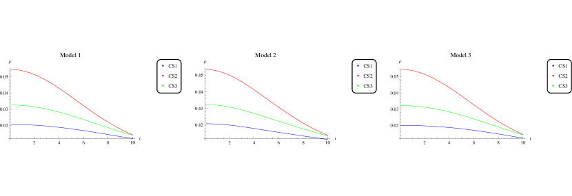
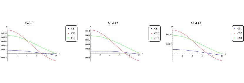
Figure 1: Density evolution of the strange star candidates with three different $f(R)$ models.

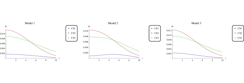
Figure 2: Radial pressure evolution of the strange stars.

Figure 3: Transverse pressure evolution of the strange stars.

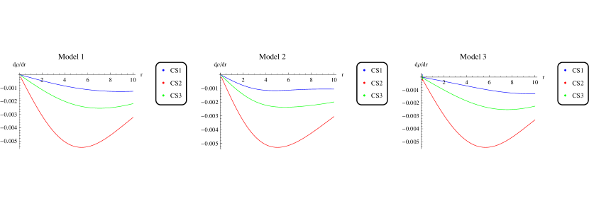
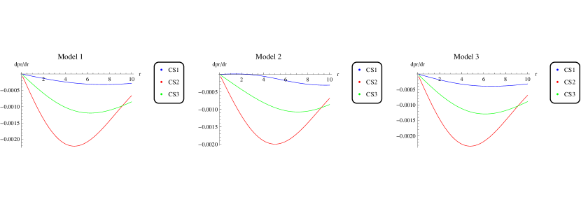
Figure 4: Behavior of $d\rho/dr$ with respect to $r$ with three different $f(R)$ models.

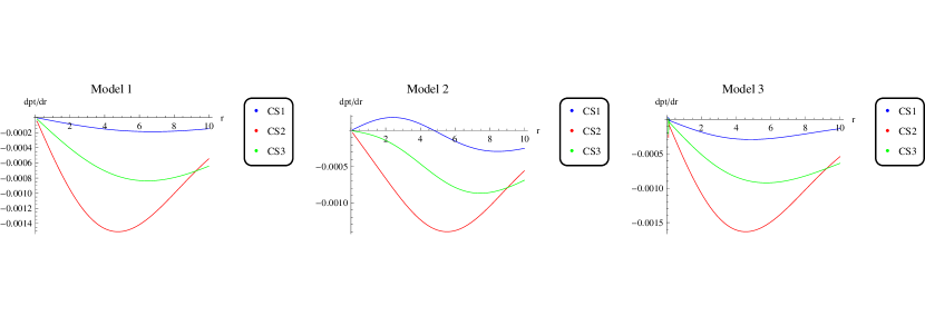
Figure 5: Behavior of $dp_{r}/dr$ with respect to $r$.

Figure 6: Behavior of $dp_{t}/dr$ with increasing $r$.

3.5 Energy Conditions

For the mathematical expressions of stress-energy tensors to represent physically acceptable matter fields, it should obey some particular constraints, widely known as ECs. These ECs have very important property that they are coordinate-invariant (independent of symmetry). Recently, Yousaf [57] explored various analytical models of the stellar filaments with dark source terms coming from cosmological constant and checked the validity regimes of ECs in order to make them physically viable. Bamba et al. [58] presented general formalism for checking the viability of ECs in modified gravity. In $f(R)$ gravity (having effective density and anisotropic pressure), the NEC and WEC are formulated as

$$\textrm{NEC}\Leftrightarrow{\rho^{\textrm{eff}}}+{p_{i}^{\textrm{eff}}}\geq 0,$$

$$\textrm{WEC}\Leftrightarrow{\rho^{\textrm{eff}}}\geq 0\text{ and }{\rho^{\textrm{eff}}}+{p_{i}^{\textrm{eff}}}\geq 0,$$

while the SEC and the dominant energy condition (DEC) yield

$$\textrm{SEC}\Leftrightarrow{\rho^{\textrm{eff}}+3{p_{r}^{\textrm{eff}}}}+2{p_{t}^{\textrm{eff}}}\geq 0\text{ and }{\rho^{\textrm{eff}}}+{p_{i}^{\textrm{eff}}}\geq 0,$$

$$\textrm{DEC}\Leftrightarrow{\rho^{\textrm{eff}}}\geq 0\text{ and }{\rho^{\textrm{eff}}}\pm{p_{i}^{\textrm{eff}}}\geq 0.$$

The evolution of all these ECs for three different compact structures are being well satisfied for all of our chosen $f(R)$ models. These are graphically shown in Figures (7)-(9).

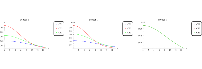
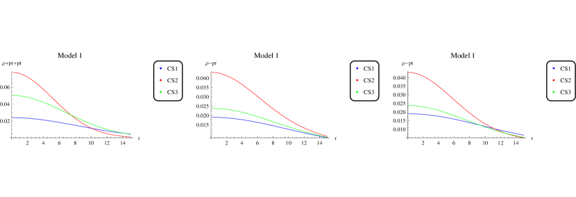
Figure 7: Viability of energy conditions for three different strange stars with dark source terms coming from $f(R)=R+\alpha{R^{2}}$.

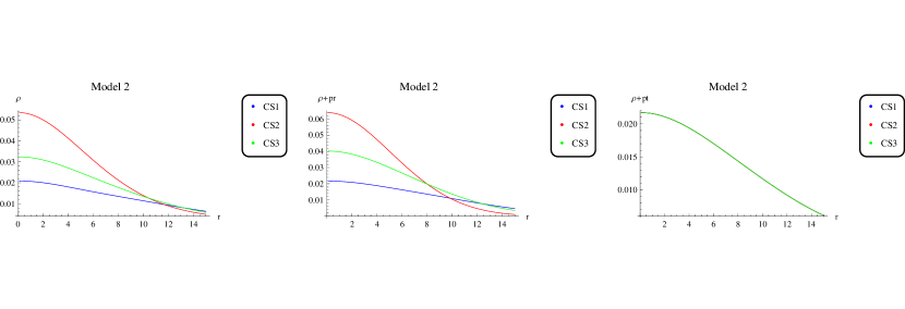
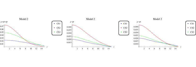
Figure 8: Viability of energy conditions for three different strange stars with $f(R)=R+\beta R\left({{e^{\left({-R/\tilde{R}}\right)}}-1}\right)$ model.

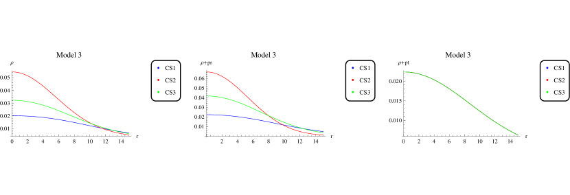
Figure 9: Viability of energy conditions for three different strange stars in the presence of $f(R)=R+\alpha{R^{2}}\left({1+\gamma R}\right)$ corrections.

3.6 TOV Equation

The TOV equation for the spherical anisotropic stellar interior is given by

$$\frac{{d{p_{r}}}}{{dr}}+\frac{{a^{\prime}(\rho+{p_{r}})}}{2}+\frac{{2({p_{r}}-{p_{t}})}}{r}=0.$$ (22)

The quantity $a^{\prime}$ is the radial derivative of the function appearing in the first metric coefficient of the line element (7). However, the quantity $a$, in general, is directly correspond to the scalar associated with the four acceleration $(a_{\beta}=aV_{\beta})$ of the anisotropic fluid and is defined as

$$a^{2}=a_{\beta}a^{\beta}$$

Equation (22) can be relabeled in terms of gravitational $(F_{g})$, hydrostatic $(F_{h})$ and anisotropic $(F_{a})$ forces as

$$F_{g}+F_{h}+F_{a}=0.$$ (23)

The values of these forces for our anisotropic spherical matter distribution have been found as follows

$$F_{g}=-Br(\rho+p_{r}),\quad F_{h}=-\frac{{d{p_{r}}}}{{dr}},\quad F_{a}=\frac{{2({p_{r}}-{p_{t}})}}{r},$$

By making use of these definitions, the behavior of these forces for the onset of hydrostatic equilibrium are shown for three strange compact stars in Figure (10). In the graphs, we have continued our analysis with different $f(R)$ theories. In Figure (10), the left plot is showing variations due to model 1, middle is for model 2 and the right plot is describing corresponding changes in principal forces due to model 3.

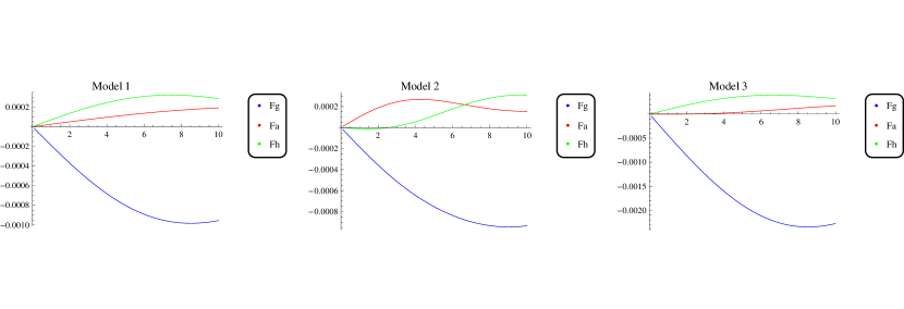
Figure 10: The plot of gravitational force ($F_{g}$), hydrostatic force ($F_{h}$) and anisotropic force $(F_{a})$ with respect to the radial coordinate r(km) and three different models.

3.7 Stability Analysis

Here, we check the stability of our stars by adopting the scheme presented by Herrera [59] that was based on the concept of cracking (or overturning). This approach states that $v^{2}_{sr}$ as well as $v^{2}_{st}$ must belong to the closed interval [0,1], where $v_{sr}$ indicates radial sound speed, while and $v_{st}$ denotes transverse sound speed defined as

$$\frac{{d{p_{r}}}}{{d\rho}}=v_{sr}^{2},\quad\frac{{d{p_{t}}}}{{d\rho}}=v_{st}^{2}.$$

The system will be dynamically stable, if $v^{2}_{st}>v^{2}_{sr}$. It has been observed that the evolution of the radial and transversal sound speeds for all three types of strange stars are within the bounds of stability for some regions. It can be seen from Figure (11) that all of our stellar structures (within the background of all $f(R)$ models) obey the following constraint

$$0<|v_{st}^{2}-v_{sr}^{2}|<1.$$

Therefore, we infer that all of our proposed model are stable in this theory. Such kind of results have been proposed by Sharif and Yousaf [60] by employing different mathematical strategy on compact stellar objects.

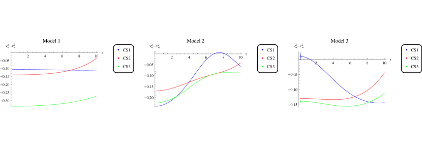
Figure 11: Variations of $v_{st}^{2}-v_{sr}^{2}$ with respect radius, $r$ (km)

3.8 Equation of State Parameter

The parameter corresponding to the equation of state (EoS) is a dimensionless term that illustrates matter state under some specific physical grounds. This parameter has its range belonging to open interval $(0,1)$. In that case, it represents radiation dominated cosmic era. For anisotropic relativistic interior, the EoS can be defined as

$$p_{r}=\omega_{r}\rho,\quad p_{t}=\omega_{t}\rho.$$

The behaviors of $\omega_{r}$ for our compact structures is shown graphically in Fig.(13). However, the similar behavior of $\omega_{t}$ can be observed for all of our observed compact structures very easily. It has been observed that maximum radius of compact objects to achieve the limit $0<\omega_{r}<1$ is $r\sim(\leq 7)$, while the constraint $0<\omega_{t}<1$ is valid for any large value of $r$. This means that $\omega_{i}>1$ near its central point. The spherically symmetric self-gravitating system would be in a radiation window at the corresponding hypersurfaces. From here, we conclude that that our relativistic bodies have a compact interior.

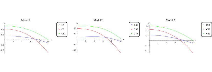
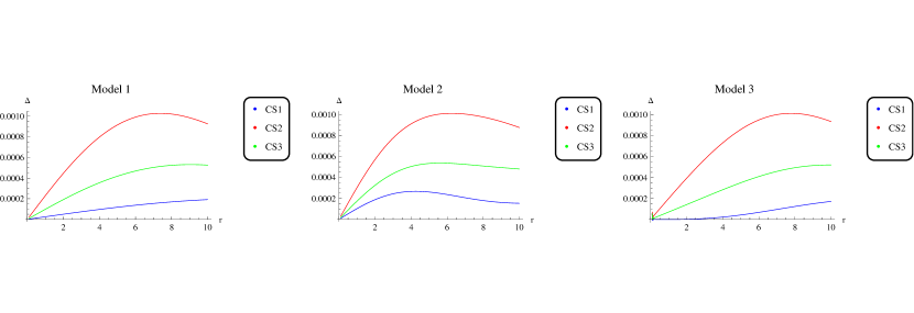
Figure 12: Variations of the radial EoS parameter, $\omega_{r}$ with respect to the radial coordinate.

Figure 13: Variations of anisotropicity, $\Delta$, with respect to $r$.

3.9 The Measurement of Anisotropy

Here, we measure the extent of anisotropy in the modeling of relativistic interiors. It is well-known that anisotropicity in the stellar system can be measured with the help of the following formula

$$\Delta=\frac{2}{r}({p_{t}}-{p_{r}}),$$ (24)

The quantity $\Delta$ is directly related to the difference $p_{t}-p_{r}$. The positivity of $\Delta$ indicates the positivity of $p_{t}-p_{r}$. Such a background suggests the outwardly drawn behavior of anisotropic pressure. However, the resultant pressure will be directly inward, once $\Delta$ is less than zero. We have drawn the anisotropic factor for our systems and obtain $\Delta>0$, thereby giving $p_{t}>p_{r}$. All these results are mentioned through plots as shown in Figure (13).

4 Summary

This paper is devoted to discuss some physical aspects of spherically symmetric compact stars in the background of metric $f(R)$ theory. We have used the Krori-Barua solutions for metric functions of spherical star whose arbitrary constants are explored over the boundary surface by matching it with suitable exterior. The arbitrary constants of the Krori-Barua solutions can be written in the form of mass and radius for any compact star. We have used the observational data of three particular star models to explore the influence of extra degrees of freedom on compact stars. For this purpose, three different physically viable $f(R)$ models are used. By using the values of these star and gravity models, we have plotted the material variables like energy density and anisotropic stresses against radial distance. It is found that as the radius of the star increases, the density tends to decrease, thereby indicating the maximum dense configurations of stellar interiors. A similar behavior is analyzed in the evolutionary phases of the tangential and radial pressures.

It is seen that $r-$derivatives of these material variables remains negative with the increasing radius for all the three models while only the $r-$derivative of tangential pressure for compact star Her X-1 has some positive value till $r=4.8$ and then becomes negative. It is also significant to note that the first derivative of these material variables vanish at $r=0$ for all the compact stars. It is found that our spherically symmetric anisotropic systems are obey NECs, WECs, SECs and DECs, hence the compact stars under the effects of extra degrees of freedom of fourth order gravity are physically valid. We have seen that the gravitational forces are overcoming the corresponding repulsive forces, thus indicating the collapsing nature of compact relativistic structures. It is well-known that a stellar system would be stable against fluctuations, if it satisfies the bounds of [0,1] for radial and tangential sound speeds. We have found that the compact star Her X-1 under the effects of second gravity model does not remain in [0,1], but Figure 11 indicates that all of our stellar models are stable (i.e., $v_{st}^{2}>v_{sr}^{2}$). Further, we have observed that the equation of state parameter lies in the interval (0,1) for all the compact stars. The anisotropic parameter remains positive which is necessary for a realistic stellar configurations. We can conclude our discussion as follows.

• The anisotropic stresses and energy density are positive throughout the star configurations.

• The $r-$derivatives of density and anisotropic stresses (i.e., density and pressure gradients) remains negative.

• All types of ECs are valid.

• The sound speeds remain within the bounds of $[0,1]$ (i.e, compact stars are stable).

• The equation of state parameter lies between 0 and 1 for each star radius.

• The measure of anisotropy remains positive at the star core.

References

- [1] S. Weinberg, Rev. Mod. Phys. 61, 1 (1989); P. J. E. Peebles and B. Ratra, Rev. Mod. Phys. 75, 559 (2003); V. Husain and B. Qureshi, Phys. Rev. Lett. 116, 061302 (2016).
- [2] D. Pietrobon, A. Balbi, and D. Marinucci, Phys. Rev. D 74, 043524 (2006); T. Giannantonio et al., Phys. Rev. D 74, 063520 (2006); A. G. Riess et al., Astrophys. J. 659, 98 (2007).
- [3] A. Qadir, H. W. Lee, and K. Y. Kim, Int. J. Mod. Phys. D 26, 1741001 (2017).
- [4] S. Capozziello and V. Faraoni, Beyond Einstein Gravity (Springer, Dordrecht, 2010).
- [5] S. Capozziello and M. De Laurentis, Phys. Rept. 509, 167 (2011) [arXiv:1108.6266 [gr-qc]].
- [6] K. Bamba, S. Capozziello, S. Nojiri and S. D. Odintsov, Astrophys. Space Sci. 342, 155 (2012) [arXiv:1205.3421 [gr-qc]];
- [7] K. Koyama,Rep. Prog. Phys. 79, 046902 (2016) [arXiv:1504.04623 [astro-ph.CO]].
- [8] Á. de la Cruz-Dombriz and D. Sáez-Gómez, Entropy 14, 1717 (2012) [arXiv:1207.2663 [gr-qc]];
- [9] K. Bamba, S. Nojiri and S. D. Odintsov, arXiv:1302.4831 [gr-qc];
- [10] K. Bamba and S. D. Odintsov, arXiv:1402.7114 [hep-th]; Symmetry 7, 220 (2015) [arXiv:1503.00442 [hep-th]].
- [11] Z. Yousaf, K. Bamba and M. Z. Bhatti, Phys. Rev. D 93, 064059 (2016) [arXiv1603.03175 [gr-qc]].
- [12] Z. Yousaf, K. Bamba and M. Z. Bhatti, Phys. Rev. D 93, 124048 (2016) [arXiv:1606.00147 [gr-qc]].
- [13] S. Nojiri, and S. D. Odintsov, eConf C 0602061, 06 (2006); Int. J. Geom. Meth. Mod. Phys. 4, 115 (2007) [hep-th/0601213].
- [14] S. Nojiri, and S. D. Odintsov, arXiv:0801.4843 [astro-ph] (2008).
- [15] S. Nojiri, and S. D. Odintsov, arXiv:0807.0685 [hep-th] (2008).
- [16] Sotiriou, T. P. and Faraoni, V.: Rev. Mod. Phys. 82, 451 (2010).
- [17] S. Nojiri, and S. D. Odintsov, Phys. Rev D 68, 123512 (2003).
- [18] Z. Yousaf, Eur. Phys. J. Plus 132, 71 (2017).
- [19] M. Sharif and Z. Yousaf, Z.: Astrophys. Space Sci. 355, 317 (2015); M. Z. Bhatti and Z. Yousaf, Int. J. Mod. Phys. D 26, 1750029 (2017); ibid. Int. J. Mod. Phys. D 26, 1750045 (2017); M. Z. Bhatti and Z. Yousaf, Eur. Phys. J. C 76, 219 (2016) [arXiv1604.01395 [gr-qc]].
- [20] T. Harko, F. S. N. Lobo, S. Nojiri and S. D. Odintsov, Phys. Rev. D 84, 024020 (2011); Z. Yousaf and M. Z. Bhatti, Eur. Phys. J. C 76, 267 (2016) [arXiv:1604.06271 [physics.gen-ph]]; M. Sharif and Z. Yousaf, Astrophys. Space Sci. 354, 471 (2014); Yousaf, Z., Bamba, K. and Bhatti, M. Z.: Phys. Rev. D 95, 024024 (2017) [arXiv:1701.03067 [gr-qc]].
- [21] S. D. Odintsov and D. Sáez-Gómez, Phys. Lett. B, 725, 437 (2013); Z. Haghani, T. Harko, F. S. N. Lobo, H. R. Sepangi and S. Shahidi, Phys. Rev. D, 88, 044023 (2013); I. Ayuso, J. B. Jiménez and Á de la Cruz-Dombriz, Phys. Rev. D, 91, 104003 (2015); Z. Yousaf, M. Z. Bhatti and U. Farwa, Class. Quantum Grav. 34, 145002 (2017).
- [22] Nojiri, S., Odintsov, S. D. and Oikonomou, V.K.: arXiv: arXiv:1705.11098 [gr-qc].
- [23] A. Sokolov, J. Exp. Theor. Phys. 79, 1137 (1980).
- [24] R. Sawyer, Phys. Rev. Lett. 29, 382 (1972)
- [25] L. Herrera, N. O. Santos, and A. Wang, Phys. Rev. D 78, 084026 (2008); L. Herrera, G. Le Denmat, and N. O. Santos, Phys. Rev. D 79, 087505 (2009).
- [26] A. Di Prisco, L. Herrera, J. Ospino, N. O. Santos, and V. M. Viña-Cervantes, Int. J. Mod. Phys. D 20, 2351 (2011); Z. Yousaf, K. Bamba and M. Z. Bhatti, Phys. Rev. D 95, 024024 (2017) [arXiv:1701.03067 [gr-qc]]; Z. Yousaf and M. Z. Bhatti, Eur. Phys. J. C 76, 267 (2016) [arXiv:1604.06271 [physics.gen-ph]].
- [27] L. Herrera, A. Di Prisco and J. Ospino, Gen. Relativ. Gravit. 85, 044022 (2012).
- [28] M. Sharif and Z. Yousaf, Astrophys. Space Sci. 357, 49 (2015); Z. Yousaf and M. Z. Bhatti, Mon. Not. R. Astron. Soc. 458, 1785 (2016) [arXiv:1612.02325 [physics.gen-ph]].
- [29] R. A. Sussman and L. G. Jaime, arXiv:1707.00191 [gr-qc].
- [30] H. Shabani and A. H. Ziaie, Eur. Phys. J. C 77, 31 (2017).
- [31] R. Garattini and G. Mandanici, Eur. Phys. J. C 77, 57 (2017).
- [32] P. K. Sahoo, P. Sahoo, B. K. Bishi, Int. J. Geom. Meth. Mod. Phys, 14, 1750097 (2017) [arXiv:1702.02469 [gr-qc]]; S. K. Sahu, S. K. Tripathy, P. K. Sahoo and A. Nath, Chin. J. Phys. 55, 862 (2017).
- [33] S. W. Hawking and G. F. R. Ellis, The Large Scale Structure of Spacetime (Cambridge University Press, Cambridge, 1979).
- [34] L. Herrera, and N. O. Santos, Phys. Rep. 286, 53 (1997); L. Herrera, A. Di Prisco, J. R. Hernandez, and N. O. Santos, Phys. Lett. A 237, 113 (1998); M. Z. Bhatti, Eur. Phys. J. Plus 131, 428 (2016); M. Z. Bhatti, Z. Yousaf and S. Hanif, Eur. Phys. J. Plus 132, 230 (2017).
- [35] G. J. Olmo, Phys. Rev. D 75, 023511 (2007); F. Briscese and E. Elizalde, Phys. Rev. D 77, 044009 (2008); Á. de la Cruz- Dombriz, A. Dobado, and A. L. Maroto, Phys. Rev. D 80, 124011 (2009); T. Clifton, P. G. Ferreira, A. Padilla, and C. Skordis, Phys. Rep. 513, 1 (2012).
- [36] S. Capozziello, M. De Laurentis, S. D. Odintsov, and A. Stabile, Phys. Rev. D 83, 064004 (2011); S. Capozziello, M. De Laurentis, I. De Martino, M. Formisano, and S. D. Odintsov, Phys. Rev. D 85, 044022 (2012).
- [37] J. A. R. Cembranos, Á. de la Cruz-Dombriz and B. M. Núñez, J. Cosmol. Astropart. Phys. 04, 021 (2012).
- [38] M. Sharif and Z. Yousaf, Eur. Phys. J. C 75, 194 (2015) [arXiv:1504.04367v1 [gr-qc]]; 351, 351 (2014); M. Sharif and Z. Yousaf, Int. J. Theor. Phys. 55, 470 (2016); M. Z. Bhatti and Z. Yousaf, Eur. Phys. J. C 76, 219 (2016) [arXiv1604.01395 [gr-qc]]; Z. Yousaf, M. Z. Bhatti and U. Farwa, Mon. Not. R. Astron. Soc. 464, 4509 (2017); M. Z. Bhatti, Z. Yousaf and S. Hanif, Phys. Dark Universe 16, 34 (2017).
- [39] J.-Q. Guo and P. S. Joshi, Phys. Rev. D 94, 044063 (2016).
- [40] J. Santos, J. S. Alcaniz, M. J. Rebouças and F. C. Carvalho, Phys. Rev. D 76, 083513 (2007).
- [41] J. Wang, Y.-B. Wu, Y.-X. Guo, W.-Q. Yang and L. Wang, Phys. Lett. B 689, 133 (2010).
- [42] M. Shiravand, Z. Haghani and S. Shahidi, arXiv: 1507.07726v2 [gr-qc].
- [43] J. Santos, M. Reboucas and J. Alcaniz, Int. J. Mod. Phys. D 19 1315 (2010) [arXiv:0807.2443].
- [44] J. Wang and K. Liao, Class. Quantum Grav. 29, 215016 (2012) [arXiv:1212.4656].
- [45] Z. Yousaf, M. Ilyas and M. Z. Bhatti, Eur. Phys. J. Plus 132, 268 (2017).
- [46] K. Atazadeh and F. Darabi, Gen. Relativ. Gravit. 46, 1664 (2014).
- [47] N. M. García, T. Harko, F. S. N. Lobo and J. P. Mimoso, Phys. Rev. D 83, 104032 (2011); S. Nojiri, S. D. Odintsov and P. V. Tretyakov, P. V.: Prog. Theor. Phys. Suppl. 172, 81 (2008).
- [48] D. Shee, S. Ghosh, F. Rahaman, B. K. Guha and S. Ray, arXiv:1612.05109v2 [physics.gen-ph]; S. K. Maurya and M. Govender, arXiv:1703.10037v1 [physics.gen-ph]; S. K. Maurya, Y. K. Gupta, S. Ray and D. Deb, Eur. Phys. J. C 76, 693 (2016) [arXiv:1607.05582 [physics.gen-ph]]; S. K. Maurya, Y. K. Gupta, S. Ray and B. Dayanandan, Eur. Phys. J. C 75, 225 (2015) [arXiv:1504.00209 [gr-qc]].
- [49] K. D. Krori and J. Barua, J. Phys. A: Math. Gen. 8, 508 (1975).
- [50] S. Weissenborn, I. Sagert, G. Pagliara, M. Hempel and J. Schaffner-Bielich, Astrophys. J. 740, L14 (2011).
- [51] F. Weber, Prog. Part. Nucl. Phys. 54, 193 (2005).
- [52] H. Bondi, Proc. R. Soc. London A 282, 303 (1964); H. A. Buchdahl, Astrophys. J. 146, 275 (1966).
- [53] M. K. Mak, P. N. D. Jr. and T. Harko, Mod. Phys. Lett. A 15, 2153 (2000) [arXiv:gr- qc/0104031].
- [54] A. A. Starobinsky, Phys. Lett. 91B, 99 (1980).
- [55] G. Cognola, E. Elizalde, S. Nojiri, S. Odintsov, L. Sebastiani and S. Zerbini, Phys. Rev. D 77, 046009 (2008) [arXiv:0712.4017 [hep-th]].
- [56] K. Bamba, C.-Q. Geng and C.-C. Lee, J. Cosmol. Astropart. Phys. 08 021 (2010) [arXiv:1005.4574 [astro-ph.CO]].
- [57] Z. Yousaf, Eur. Phys. J. Plus 132, 276 (2017).
- [58] K. Bamba, M. Ilyas, M. Z. Bhatti and Z. Yousaf, Gen. Relativ. Gravit. 49, 112 (2017) [arXiv: 1707.07386 [gr-qc].
- [59] L. Herrera, Phys. Lett. A 165, 206 (1992).
- [60] M. Sharif and Z. Yousaf, J. Cosmol. Astropart. Phys. 06, 019 (2014); M. Sharif and Z. Yousaf, Astrophys. Space Sci. 354, 431 (2014); M. Sharif and Z. Yousaf, Gen. Relativ. Gravit. 47, 48 (2015).